跳到论文正文
W Papers独立论文阅读器 arXiv:2106.06186 论文正文 计算阅读时间 · 0%
引用这篇论文根据当前论文元数据生成,正式投稿前建议核对。


License: CC BY 4.0
arXiv:2106.06186v2 [math.OC] 21 Aug 2023

Real-Value Power-Voltage Formulations of, and Bounds for, Three-Wire Unbalanced Optimal Power Flow

Frederik Geth  and  Hakan Ergun Note: Dr. Geth is with GridQube, Springfield (Brisbane), Queensland, Australia. frederik.geth [at] gridqube.com Note: Dr. Ergun is with KU Leuven, Kasteelpark Arenberg 10, Heverlee, Belgium and EnergyVille, Thor Park 8310, Belgium. hakan.ergun [at] kuleuven.be
Abstract

Unbalanced optimal power flow refers to a class of optimization problems subject to the steady state physics of three-phase power grids with nonnegligible phase unbalance. Significant progress on this problem has been made on the mathematical modelling side of unbalanced OPF, however there is a lack of information on implementation aspects as well as data sets for benchmarking. One of the key problems is the lack of definitions of current and voltage bounds across different classes of representations of the power flow equations. Therefore, this tutorial-style paper summarizes the structural features of the unbalanced (optimal) power problem for three-phase systems. The resulting nonlinear complex-value matrix formulations are presented for both the bus injection and branch flow formulation frameworks, which typically cannot be implemented as-is in optimization toolboxes. Therefore, this paper also derives the equivalent real-value formulations, and discusses challenges related to the implementation in optimization modeling toolboxes. The derived formulations can be re-used easily for continuous and discrete optimization problems in distribution networks for a variety of operational and planning problems. Finally, bounds are derived for all variables involved, to further the development of benchmarks for unbalanced optimal power flow, where consensus on bound semantics is a pressing need. We believe benchmarks remain a cornerstone for the development and validation of scalable and reproducible optimization models and tools. The soundness of the derivations is confirmed through numerical experiments, validated w.r.t. OpenDSS for IEEE test feeders with 3×33\times 3 impedance matrices.

Nomenclature

This article depends on the definition of a variety of scalar, vector and matrix parameters and variables related to grid buses and branches (see Tables 1-5). The core variables are current, voltage and power, whereas parameters are mainly impedance and variable bounds. Fig. 1 summarizes the variables and parameters defined in the fundamental 3×33\times 3 branch model for which the well known The Π\Pi-equivalent model used. With respect to balance networks, both series and shunt elements are represented by full complex-valued matrices including the mutual impedance coupling between the conductors. Using the Π\Pi-equivalent model, the branch current 𝐈l​i​j{\color[rgb]{0,0,1}\mathbf{I}_{{l}{i}{j}}} can be split into a series component 𝐈l​i​js{\color[rgb]{0,0,1}\mathbf{I}_{{l}{i}{j}}^{\text{{s}}}} and a shunt component 𝐈l​i​jsh{\color[rgb]{0,0,1}\mathbf{I}_{{l}{i}{j}}^{\text{{sh}}}}, respectively. All circuit element voltages are defined w.r.t. (local) ground voltage Ui,g=0​V{\color[rgb]{0,0,1}U_{{i},{g}}}=0\,V.

Figure 1: Unbalanced 3×33\times 3 Π\Pi-model branch in voltage and current variables.

Table 1 illustrates typography and mathematical notation used throughout; Table 2 defines sets and indices; Table 3 defines parameters; Table 4 defines typical engineering variables; Table 5 defines lifted variables. Black and red colors indicate real-valued variables and parameters, respectively. Blue and brown colors are used for complex-valued variables and parameters, respectively.

Table 1: Typography and mathematical notation

\IEEEeqnarraystrutmode]Lsxr​e​a​l​s​c​a​l​a​r​v​a​r​i​a​b​l​e𝐗r​e​a​l​v​e​c​t​o​r​o​r​m​a​t​r​i​x​v​a​r​i​a​b​l​exc​o​m​p​l​e​x​s​c​a​l​a​r​v​a​r​i​a​b​l​e𝐗c​o​m​p​l​e​x​v​e​c​t​o​r​o​r​m​a​t​r​i​x​v​a​r​i​a​b​l​exr​e​a​l​s​c​a​l​a​r​p​a​r​a​m​e​t​e​r𝐗r​e​a​l​v​e​c​t​o​r​o​r​m​a​t​r​i​x​p​a​r​a​m​e​t​e​rxc​o​m​p​l​e​x​s​c​a​l​a​r​p​a​r​a​m​e​t​e​r𝐗c​o​m​p​l​e​x​v​e​c​t​o​r​o​r​m​a​t​r​i​x​p​a​r​a​m​e​t​e​r𝒳s​e​t𝐗Tt​r​a​n​s​p​o​s​e​o​f​X𝐗∗c​o​n​j​u​g​a​t​e​o​f​X𝐗H=(𝐗∗)Tc​o​n​j​u​g​a​t​e​t​r​a​n​s​p​o​s​e​o​f​X∘e​l​e​m​e​n​t−w​i​s​e​m​u​l​t​i​p​l​i​c​a​t​i​o​n⊘e​l​e​m​e​n​t−w​i​s​e​d​i​v​i​s​i​o​nji​m​a​g​i​n​a​r​y​u​n​i​t,s​a​t​i​s​f​i​e​s​ j^2 = -1a​∠​bp​o​l​a​r​n​o​t​a​t​i​o​n​o​f​c​o​m​p​l​e​x​n​u​m​b​e​r​ a ⋅e^jbℝn×ms​e​t​o​f​r​e​a​l​n×m​m​a​t​r​i​c​e​sℂn×ms​e​t​o​f​c​o​m​p​l​e​x​n×m​m​a​t​r​i​c​e​sℍn⊂ℂn×ns​e​t​o​f​H​e​r​m​i​t​i​a​n​n×n​m​a​t​r​i​c​e​sdiag⁡(𝐗)extractdiagonalofX,diag:  C^n×n  → C^n×1  \begin{IEEEeqnarraybox}[]{[}\IEEEeqnarraystrutmode]{Ls}x&realscalarvariable\\ \mathbf{X}&realvectorormatrixvariable\\ {\color[rgb]{0,0,1}x}&complexscalarvariable\\ {\color[rgb]{0,0,1}\mathbf{X}}&complexvectorormatrixvariable\\ {\color[rgb]{1,0,0}x}&realscalarparameter\\ {\color[rgb]{1,0,0}\mathbf{X}}&realvectorormatrixparameter\\ {\color[rgb]{0.75,0.5,0.25}x}&complexscalarparameter\\ {\color[rgb]{0.75,0.5,0.25}\mathbf{X}}&complexvectorormatrixparameter\\ \mathcal{X}&set\\ \mathbf{X}^{\text{T}}&transposeof$\mathbf{X}$\\ {\color[rgb]{0,0,1}\mathbf{X}}^{*}&conjugateof${\color[rgb]{0,0,1}\mathbf{X}}$\\ {\color[rgb]{0,0,1}\mathbf{X}}^{\text{H}}={\color[rgb]{0,0,1}(\mathbf{X}^{*})}^{\text{T}}&conjugatetransposeof${\color[rgb]{0,0,1}\mathbf{X}}$\\ \circ&element-wisemultiplication\\ \oslash&element-wisedivision\\ {\color[rgb]{1,0,0}j}&imaginaryunit,satisfies$ {\color[rgb]{1,0,0}j}^2 = -1$\\ a{\color[rgb]{1,0,0}\angle}b&polarnotationofcomplexnumber$ a \cdot e^{{\color[rgb]{1,0,0}j}b}$\\ {\color[rgb]{0.25,0.25,0.25}\mathbb{R}^{n\times m}}&setofreal$n\times m$matrices\\ {\color[rgb]{0.25,0.25,0.25}\mathbb{C}^{n\times m}}&setofcomplex$n\times m$matrices\\ {\color[rgb]{0.25,0.25,0.25}\mathbb{H}^{n}}\subset{\color[rgb]{0.25,0.25,0.25}\mathbb{C}^{n\times n}}&setofHermitian$n\times n$matrices\\ \diag({\color[rgb]{0,0,1}\mathbf{X}})&extractdiagonalof${\color[rgb]{0,0,1}\mathbf{X}}$,$\diag: {\color[rgb]{0.25,0.25,0.25} \mathbb{C}^{n\times n} } \rightarrow{\color[rgb]{0.25,0.25,0.25} \mathbb{C}^{n\times 1} } $\\ \hline\cr\end{IEEEeqnarraybox}

Table 2: Sets and indices
Phases p,q∈𝒫={a,b,c}p,q\in{\color[rgb]{1,0,0}\mathcal{P}}=\{{a},{b},{c}\}
Branches l∈𝒥{l}\in{\color[rgb]{1,0,0}\mathcal{J}}
Buses i∈ℐ{i}\in{\color[rgb]{1,0,0}\mathcal{I}}
Topology (forward) l​i​j∈𝒯           ⊆𝒥×ℐ×ℐ{l}{i}{j}\in{\color[rgb]{1,0,0}\mathcal{T}^{\parbox{2.84544pt}{\hbox to3.25pt{\vbox to0.4pt{\pgfpicture\makeatletter\hbox{\hskip 0.2pt\lower-0.2pt\hbox to0.0pt{\lxSVG@begingroup@{_scopebegin} \lxSVG@begingroup@{stroke} \lxSVG@begingroup@{fill} \lxSVG@setlinewidth{\the\pgflinewidth}\lxSVG@begingroup@{stroke-width} \lx@inpgf@ignorespaces\nullfont\hbox to0.0pt{\lxSVG@begingroup@{_scopebegin} {{}{{}}{} {{\lx@inpgf@ignorespaces}{}}{}{}{{ {\lxSVG@setlinewidth{\the\pgflinewidth}\lx@inpgf@ignorespaces\lxSVG@setdash{0.0pt}\lx@inpgf@ignorespaces\lxSVG@roundcap\lx@inpgf@ignorespaces\lxSVG@roundjoin\lx@inpgf@ignorespaces{} {}{}{} {}{}{} \lxSVG@stroke}} }{}{}{{}}\lxSVG@stroke\lxSVG@drawpath@unclipped{M 0 0 L 3.3 0}{fill:none} {{}{{}}{}{}{{}}{{{\lx@inpgf@ignorespaces}}{{{\lx@inpgf@ignorespaces}}{\lxSVG@begingroup@{_scopebegin} \lxSVG@transformcm{1.0}{0.0}{0.0}{1.0}{2.38528pt}{0.0pt}\lxSVG@begingroup@{transform} \lxSVG@begingroup@{_scopebegin} \lxSVG@begingroup@{stroke-width} \lxSVG@begingroup@{stroke-dasharray,stroke-dashoffset} \lxSVG@begingroup@{stroke-linecap} \lxSVG@begingroup@{stroke-linejoin} \lxSVG@drawpath@unclipped{M -1.66 2.21 C -1.52 1.38 0 0.14 0.42 0 C 0 -0.14 -1.52 -1.38 -1.66 -2.21}{fill:none} \lxSVG@closescope \lxSVG@closescope }}{{\lx@inpgf@ignorespaces}}}}\lx@inpgf@ignorespaces } \lxSVG@closescope {\lx@inpgf@ignorespaces}{\lx@inpgf@ignorespaces}{\lx@inpgf@ignorespaces}\hss}\lxSVG@discardpath\lxSVG@closescope \hss}}\lxSVG@closescope\endpgfpicture}}}}}\subseteq{\color[rgb]{1,0,0}\mathcal{J}}\times{\color[rgb]{1,0,0}\mathcal{I}}\times{\color[rgb]{1,0,0}\mathcal{I}}
Topology (reverse) l​i​j∈𝒯           ={l​j​i|l​i​j∈𝒯           }{l}{i}{j}\in{\color[rgb]{1,0,0}\mathcal{T}^{\parbox{2.84544pt}{\hbox to3.25pt{\vbox to0.4pt{\pgfpicture\makeatletter\hbox{\hskip 0.2pt\lower-0.2pt\hbox to0.0pt{\lxSVG@begingroup@{_scopebegin} \lxSVG@begingroup@{stroke} \lxSVG@begingroup@{fill} \lxSVG@setlinewidth{\the\pgflinewidth}\lxSVG@begingroup@{stroke-width} \lx@inpgf@ignorespaces\nullfont\hbox to0.0pt{\lxSVG@begingroup@{_scopebegin} {{}{{}}{} {{\lx@inpgf@ignorespaces}{}}{}{}{}{}{}{{}}\lxSVG@stroke\lxSVG@drawpath@unclipped{M 0.64 0 L 3.94 0}{fill:none} {{}{{}}{}{}{{}}{{{\lx@inpgf@ignorespaces}}{{{\lx@inpgf@ignorespaces}}{\lxSVG@begingroup@{_scopebegin} \lxSVG@transformcm{-1.0}{0.0}{0.0}{-1.0}{0.45999pt}{0.0pt}\lxSVG@begingroup@{transform} \lxSVG@begingroup@{_scopebegin} \lxSVG@begingroup@{stroke-width} \lxSVG@begingroup@{stroke-dasharray,stroke-dashoffset} \lxSVG@begingroup@{stroke-linecap} \lxSVG@begingroup@{stroke-linejoin} \lxSVG@drawpath@unclipped{M -1.66 2.21 C -1.52 1.38 0 0.14 0.42 0 C 0 -0.14 -1.52 -1.38 -1.66 -2.21}{fill:none} \lxSVG@closescope \lxSVG@closescope }}{{\lx@inpgf@ignorespaces}}}}\lx@inpgf@ignorespaces } \lxSVG@closescope {\lx@inpgf@ignorespaces}{\lx@inpgf@ignorespaces}{\lx@inpgf@ignorespaces}\hss}\lxSVG@discardpath\lxSVG@closescope \hss}}\lxSVG@closescope\endpgfpicture}}}}}=\{{l}{j}{i}\,|\,{l}{i}{j}\in{\color[rgb]{1,0,0}\mathcal{T}^{\parbox{2.84544pt}{\hbox to3.25pt{\vbox to0.4pt{\pgfpicture\makeatletter\hbox{\hskip 0.2pt\lower-0.2pt\hbox to0.0pt{\lxSVG@begingroup@{_scopebegin} \lxSVG@begingroup@{stroke} \lxSVG@begingroup@{fill} \lxSVG@setlinewidth{\the\pgflinewidth}\lxSVG@begingroup@{stroke-width} \lx@inpgf@ignorespaces\nullfont\hbox to0.0pt{\lxSVG@begingroup@{_scopebegin} {{}{{}}{} {{\lx@inpgf@ignorespaces}{}}{}{}{}{}{}{{}}\lxSVG@stroke\lxSVG@drawpath@unclipped{M 0 0 L 3.3 0}{fill:none} {{}{{}}{}{}{{}}{{{\lx@inpgf@ignorespaces}}{{{\lx@inpgf@ignorespaces}}{\lxSVG@begingroup@{_scopebegin} \lxSVG@transformcm{1.0}{0.0}{0.0}{1.0}{2.38528pt}{0.0pt}\lxSVG@begingroup@{transform} \lxSVG@begingroup@{_scopebegin} \lxSVG@begingroup@{stroke-width} \lxSVG@begingroup@{stroke-dasharray,stroke-dashoffset} \lxSVG@begingroup@{stroke-linecap} \lxSVG@begingroup@{stroke-linejoin} \lxSVG@drawpath@unclipped{M -1.66 2.21 C -1.52 1.38 0 0.14 0.42 0 C 0 -0.14 -1.52 -1.38 -1.66 -2.21}{fill:none} \lxSVG@closescope \lxSVG@closescope }}{{\lx@inpgf@ignorespaces}}}}\lx@inpgf@ignorespaces } \lxSVG@closescope {\lx@inpgf@ignorespaces}{\lx@inpgf@ignorespaces}{\lx@inpgf@ignorespaces}\hss}\lxSVG@discardpath\lxSVG@closescope \hss}}\lxSVG@closescope\endpgfpicture}}}}}\}
Topology l​i​j∈𝒯=𝒯           ∪𝒯           {l}{i}{j}\in{\color[rgb]{1,0,0}\mathcal{T}}={\color[rgb]{1,0,0}\mathcal{T}^{\parbox{2.84544pt}{\hbox to3.25pt{\vbox to0.4pt{\pgfpicture\makeatletter\hbox{\hskip 0.2pt\lower-0.2pt\hbox to0.0pt{\lxSVG@begingroup@{_scopebegin} \lxSVG@begingroup@{stroke} \lxSVG@begingroup@{fill} \lxSVG@setlinewidth{\the\pgflinewidth}\lxSVG@begingroup@{stroke-width} \lx@inpgf@ignorespaces\nullfont\hbox to0.0pt{\lxSVG@begingroup@{_scopebegin} {{}{{}}{} {{\lx@inpgf@ignorespaces}{}}{}{}{}{}{}{{}}\lxSVG@stroke\lxSVG@drawpath@unclipped{M 0 0 L 3.3 0}{fill:none} {{}{{}}{}{}{{}}{{{\lx@inpgf@ignorespaces}}{{{\lx@inpgf@ignorespaces}}{\lxSVG@begingroup@{_scopebegin} \lxSVG@transformcm{1.0}{0.0}{0.0}{1.0}{2.38528pt}{0.0pt}\lxSVG@begingroup@{transform} \lxSVG@begingroup@{_scopebegin} \lxSVG@begingroup@{stroke-width} \lxSVG@begingroup@{stroke-dasharray,stroke-dashoffset} \lxSVG@begingroup@{stroke-linecap} \lxSVG@begingroup@{stroke-linejoin} \lxSVG@drawpath@unclipped{M -1.66 2.21 C -1.52 1.38 0 0.14 0.42 0 C 0 -0.14 -1.52 -1.38 -1.66 -2.21}{fill:none} \lxSVG@closescope \lxSVG@closescope }}{{\lx@inpgf@ignorespaces}}}}\lx@inpgf@ignorespaces } \lxSVG@closescope {\lx@inpgf@ignorespaces}{\lx@inpgf@ignorespaces}{\lx@inpgf@ignorespaces}\hss}\lxSVG@discardpath\lxSVG@closescope \hss}}\lxSVG@closescope\endpgfpicture}}}}}\cup{\color[rgb]{1,0,0}\mathcal{T}^{\parbox{2.84544pt}{\hbox to3.25pt{\vbox to0.4pt{\pgfpicture\makeatletter\hbox{\hskip 0.2pt\lower-0.2pt\hbox to0.0pt{\lxSVG@begingroup@{_scopebegin} \lxSVG@begingroup@{stroke} \lxSVG@begingroup@{fill} \lxSVG@setlinewidth{\the\pgflinewidth}\lxSVG@begingroup@{stroke-width} \lx@inpgf@ignorespaces\nullfont\hbox to0.0pt{\lxSVG@begingroup@{_scopebegin} {{}{{}}{} {{\lx@inpgf@ignorespaces}{}}{}{}{}{}{}{{}}\lxSVG@stroke\lxSVG@drawpath@unclipped{M 0.64 0 L 3.94 0}{fill:none} {{}{{}}{}{}{{}}{{{\lx@inpgf@ignorespaces}}{{{\lx@inpgf@ignorespaces}}{\lxSVG@begingroup@{_scopebegin} \lxSVG@transformcm{-1.0}{0.0}{0.0}{-1.0}{0.45999pt}{0.0pt}\lxSVG@begingroup@{transform} \lxSVG@begingroup@{_scopebegin} \lxSVG@begingroup@{stroke-width} \lxSVG@begingroup@{stroke-dasharray,stroke-dashoffset} \lxSVG@begingroup@{stroke-linecap} \lxSVG@begingroup@{stroke-linejoin} \lxSVG@drawpath@unclipped{M -1.66 2.21 C -1.52 1.38 0 0.14 0.42 0 C 0 -0.14 -1.52 -1.38 -1.66 -2.21}{fill:none} \lxSVG@closescope \lxSVG@closescope }}{{\lx@inpgf@ignorespaces}}}}\lx@inpgf@ignorespaces } \lxSVG@closescope {\lx@inpgf@ignorespaces}{\lx@inpgf@ignorespaces}{\lx@inpgf@ignorespaces}\hss}\lxSVG@discardpath\lxSVG@closescope \hss}}\lxSVG@closescope\endpgfpicture}}}}}
Bus pairs i​j∈ℬ={i​j|l​i​j∈𝒯           }⊆ℐ×ℐ{i}{j}\in{\color[rgb]{1,0,0}\mathcal{B}}=\{ij\,|\,{l}{i}{j}\in{\color[rgb]{1,0,0}\mathcal{T}^{\parbox{2.84544pt}{\hbox to3.25pt{\vbox to0.4pt{\pgfpicture\makeatletter\hbox{\hskip 0.2pt\lower-0.2pt\hbox to0.0pt{\lxSVG@begingroup@{_scopebegin} \lxSVG@begingroup@{stroke} \lxSVG@begingroup@{fill} \lxSVG@setlinewidth{\the\pgflinewidth}\lxSVG@begingroup@{stroke-width} \lx@inpgf@ignorespaces\nullfont\hbox to0.0pt{\lxSVG@begingroup@{_scopebegin} {{}{{}}{} {{\lx@inpgf@ignorespaces}{}}{}{}{}{}{}{{}}\lxSVG@stroke\lxSVG@drawpath@unclipped{M 0 0 L 3.3 0}{fill:none} {{}{{}}{}{}{{}}{{{\lx@inpgf@ignorespaces}}{{{\lx@inpgf@ignorespaces}}{\lxSVG@begingroup@{_scopebegin} \lxSVG@transformcm{1.0}{0.0}{0.0}{1.0}{2.38528pt}{0.0pt}\lxSVG@begingroup@{transform} \lxSVG@begingroup@{_scopebegin} \lxSVG@begingroup@{stroke-width} \lxSVG@begingroup@{stroke-dasharray,stroke-dashoffset} \lxSVG@begingroup@{stroke-linecap} \lxSVG@begingroup@{stroke-linejoin} \lxSVG@drawpath@unclipped{M -1.66 2.21 C -1.52 1.38 0 0.14 0.42 0 C 0 -0.14 -1.52 -1.38 -1.66 -2.21}{fill:none} \lxSVG@closescope \lxSVG@closescope }}{{\lx@inpgf@ignorespaces}}}}\lx@inpgf@ignorespaces } \lxSVG@closescope {\lx@inpgf@ignorespaces}{\lx@inpgf@ignorespaces}{\lx@inpgf@ignorespaces}\hss}\lxSVG@discardpath\lxSVG@closescope \hss}}\lxSVG@closescope\endpgfpicture}}}}}\}\subseteq{\color[rgb]{1,0,0}\mathcal{I}}\times{\color[rgb]{1,0,0}\mathcal{I}}
Units u∈𝒰{u}\in{\color[rgb]{1,0,0}\mathcal{U}}
Unit connectivity u​i∈𝒯units⊆𝒰×ℐ{u}{i}\in{\color[rgb]{1,0,0}\mathcal{T^{\text{units}}}}\subseteq{\color[rgb]{1,0,0}\mathcal{U}}\times{\color[rgb]{1,0,0}\mathcal{I}}
Shunt connectivity h​i∈𝒯shunts⊆𝒰×ℐ{h}{i}\in{\color[rgb]{1,0,0}\mathcal{T^{\text{shunts}}}}\subseteq{\color[rgb]{1,0,0}\mathcal{U}}\times{\color[rgb]{1,0,0}\mathcal{I}}
Table 3: Parameters
Bus voltage magnitude min./max. (V) 𝐔imin,𝐔imax∈ℝ|𝒫|×1{\color[rgb]{1,0,0}\mathbf{U}_{{i}}^{\text{min}}},{\color[rgb]{1,0,0}\mathbf{U}_{{i}}^{\text{max}}}\in{\color[rgb]{0.25,0.25,0.25}\mathbb{R}^{|{\color[rgb]{1,0,0}\mathcal{P}}|\times 1}}
Bus phase angle diff. min./max. (rad) 𝚯imin,𝚯imax∈ℝ|𝒫|×1{\color[rgb]{1,0,0}\mathbf{\Theta}_{{i}}^{\text{min}}},{\color[rgb]{1,0,0}\mathbf{\Theta}_{{i}}^{\text{max}}}\in{\color[rgb]{0.25,0.25,0.25}\mathbb{R}^{|{\color[rgb]{1,0,0}\mathcal{P}}|\times 1}}
Branch current rating (A) 𝐈l​i​jrated∈ℝ|𝒫|×1{\color[rgb]{1,0,0}\mathbf{I}_{{l}{i}{j}}^{\text{rated}}}\in{\color[rgb]{0.25,0.25,0.25}\mathbb{R}^{|{\color[rgb]{1,0,0}\mathcal{P}}|\times 1}}
Branch apparent power rating (VA) 𝐒l​i​jrated∈ℝ|𝒫|×1{\color[rgb]{1,0,0}\mathbf{S}_{{l}{i}{j}}^{\text{rated}}}\in{\color[rgb]{0.25,0.25,0.25}\mathbb{R}^{|{\color[rgb]{1,0,0}\mathcal{P}}|\times 1}}
Branch series impedance (Ω\Omega) 𝐳ls∈ℂ|𝒫|×|𝒫|{\color[rgb]{0.75,0.5,0.25}\mathbf{z}_{{l}}^{\text{{s}}}}\in{\color[rgb]{0.25,0.25,0.25}\mathbb{C}^{|{\color[rgb]{1,0,0}\mathcal{P}}|\times|{\color[rgb]{1,0,0}\mathcal{P}}|}}
Branch series admittance (S) 𝐲ls∈ℂ|𝒫|×|𝒫|{\color[rgb]{0.75,0.5,0.25}\mathbf{y}_{{l}}^{\text{{s}}}}\in{\color[rgb]{0.25,0.25,0.25}\mathbb{C}^{|{\color[rgb]{1,0,0}\mathcal{P}}|\times|{\color[rgb]{1,0,0}\mathcal{P}}|}}
Branch from/to shunt admittance (S) 𝐲l​i​jsh,𝐲l​j​ish∈ℂ|𝒫|×|𝒫|{\color[rgb]{0.75,0.5,0.25}\mathbf{y}_{{l}{i}{j}}^{\text{{sh}}}},{\color[rgb]{0.75,0.5,0.25}\mathbf{y}_{{l}{j}{i}}^{\text{{sh}}}}\in{\color[rgb]{0.25,0.25,0.25}\mathbb{C}^{|{\color[rgb]{1,0,0}\mathcal{P}}|\times|{\color[rgb]{1,0,0}\mathcal{P}}|}}
Bus pair angle diff. min./max. (rad) 𝚯i​jmin,𝚯i​jmax∈ℝ|𝒫|×1{\color[rgb]{1,0,0}\mathbf{\Theta}_{{i}{j}}^{\text{min}}},{\color[rgb]{1,0,0}\mathbf{\Theta}_{{i}{j}}^{\text{max}}}\in{\color[rgb]{0.25,0.25,0.25}\mathbb{R}^{|{\color[rgb]{1,0,0}\mathcal{P}}|\times 1}}
Bus shunt admittance (S) 𝐲h∈ℂ|𝒫|×|𝒫|{\color[rgb]{0.75,0.5,0.25}\mathbf{y}_{{h}}}\in{\color[rgb]{0.25,0.25,0.25}\mathbb{C}^{|{\color[rgb]{1,0,0}\mathcal{P}}|\times|{\color[rgb]{1,0,0}\mathcal{P}}|}}
Unit current rating (A) 𝐈urated∈ℝ|𝒫|×1{\color[rgb]{1,0,0}\mathbf{I}_{{u}}^{\text{rated}}}\in{\color[rgb]{0.25,0.25,0.25}\mathbb{R}^{|{\color[rgb]{1,0,0}\mathcal{P}}|\times 1}}
Unit active power bounds (W) 𝐏umin,𝐏umax∈ℝ|𝒫|×1{\color[rgb]{1,0,0}\mathbf{P}_{{u}}^{\text{min}}},{\color[rgb]{1,0,0}\mathbf{P}_{{u}}^{\text{max}}}\in{\color[rgb]{0.25,0.25,0.25}\mathbb{R}^{|{\color[rgb]{1,0,0}\mathcal{P}}|\times 1}}
Unit reactive power bounds (var) 𝐐umin,𝐐umax∈ℝ|𝒫|×1{\color[rgb]{1,0,0}\mathbf{Q}_{{u}}^{\text{min}}},{\color[rgb]{1,0,0}\mathbf{Q}_{{u}}^{\text{max}}}\in{\color[rgb]{0.25,0.25,0.25}\mathbb{R}^{|{\color[rgb]{1,0,0}\mathcal{P}}|\times 1}}
Table 4: Optimization variables
Bus voltage (V) 𝐔i,𝐔j∈ℂ|𝒫|×1{\color[rgb]{0,0,1}\mathbf{U}_{{i}}},{\color[rgb]{0,0,1}\mathbf{U}_{{j}}}\in{\color[rgb]{0.25,0.25,0.25}\mathbb{C}^{|{\color[rgb]{1,0,0}\mathcal{P}}|\times 1}}
Branch current (A) 𝐈l​i​j,𝐈l​j​i∈ℂ|𝒫|×1{\color[rgb]{0,0,1}\mathbf{I}_{{l}{i}{j}}},{\color[rgb]{0,0,1}\mathbf{I}_{{l}{j}{i}}}\in{\color[rgb]{0.25,0.25,0.25}\mathbb{C}^{|{\color[rgb]{1,0,0}\mathcal{P}}|\times 1}}
Branch series current (A) 𝐈l​i​js,𝐈l​j​is∈ℂ|𝒫|×1{\color[rgb]{0,0,1}\mathbf{I}_{{l}{i}{j}}^{\text{{s}}}},{\color[rgb]{0,0,1}\mathbf{I}_{{l}{j}{i}}^{\text{{s}}}}\in{\color[rgb]{0.25,0.25,0.25}\mathbb{C}^{|{\color[rgb]{1,0,0}\mathcal{P}}|\times 1}}
Branch shunt current (A) 𝐈l​i​jsh,𝐈l​j​ish∈ℂ|𝒫|×1{\color[rgb]{0,0,1}\mathbf{I}_{{l}{i}{j}}^{\text{{sh}}}},{\color[rgb]{0,0,1}\mathbf{I}_{{l}{j}{i}}^{\text{{sh}}}}\in{\color[rgb]{0.25,0.25,0.25}\mathbb{C}^{|{\color[rgb]{1,0,0}\mathcal{P}}|\times 1}}
Branch power flow (W) 𝐒l​i​j,𝐒l​j​i∈ℂ|𝒫|×|𝒫|{\color[rgb]{0,0,1}\mathbf{S}_{{l}{i}{j}}},{\color[rgb]{0,0,1}\mathbf{S}_{{l}{j}{i}}}\in{\color[rgb]{0.25,0.25,0.25}\mathbb{C}^{|{\color[rgb]{1,0,0}\mathcal{P}}|\times|{\color[rgb]{1,0,0}\mathcal{P}}|}}
Branch series power flow (W) 𝐒l​i​js,𝐒l​j​is∈ℂ|𝒫|×|𝒫|{\color[rgb]{0,0,1}\mathbf{S}_{{l}{i}{j}}^{\text{{s}}}},{\color[rgb]{0,0,1}\mathbf{S}_{{l}{j}{i}}^{\text{{s}}}}\in{\color[rgb]{0.25,0.25,0.25}\mathbb{C}^{|{\color[rgb]{1,0,0}\mathcal{P}}|\times|{\color[rgb]{1,0,0}\mathcal{P}}|}}
Unit current (A) 𝐈u∈ℂ|𝒫|×1{\color[rgb]{0,0,1}\mathbf{I}_{{u}}}\in{\color[rgb]{0.25,0.25,0.25}\mathbb{C}^{|{\color[rgb]{1,0,0}\mathcal{P}}|\times 1}}
Unit power (W) 𝐒u∈ℂ|𝒫|×|𝒫|{\color[rgb]{0,0,1}\mathbf{S}_{{u}}}\in{\color[rgb]{0.25,0.25,0.25}\mathbb{C}^{|{\color[rgb]{1,0,0}\mathcal{P}}|\times|{\color[rgb]{1,0,0}\mathcal{P}}|}}
Table 5: Lifted optimization variables
\IEEEeqnarraystrutmode]sLBusvoltageproduct(V^2)𝐖i,𝐖j∈ℍ|𝒫|B​u​s​p​a​i​r​v​o​l​t​a​g​e​p​r​o​d​u​c​t​(V​^2)𝐖i​j,𝐖j​i∈ℂ|𝒫|×|𝒫|B​r​a​n​c​h​c​u​r​r​e​n​t​p​r​o​d​u​c​t​(A​^2)𝐋l​i​j,𝐋l​j​i∈ℍ|𝒫|B​r​a​n​c​h​s​e​r​i​e​s​c​u​r​r​e​n​t​p​r​o​d​u​c​t​(A​^2)𝐋ls∈ℍ|𝒫|S​y​s​t​e​m​v​o​l​t​a​g​e​p​r​o​d​u​c​t​(V​^2)𝐌∈ℍ|ℬ|​|𝒫|B​u​s​p​a​i​r​v​o​l​t​a​g​e​p​r​o​d​u​c​t​(V​^2)𝐌i​j∈ℍ2​|𝒫|B​r​a​n​c​h​v​o​l​t​a​g​e−c​u​r​r​e​n​t​p​r​o​d​u​c​t​(m​i​x)𝐌l​i​j∈ℍ2​|𝒫|\begin{IEEEeqnarraybox}[]{[}\IEEEeqnarraystrutmode]{sL}Busvoltageproduct(V$^2$)&{\color[rgb]{0,0,1}\mathbf{W}_{{i}}},{\color[rgb]{0,0,1}\mathbf{W}_{{j}}}\in{\color[rgb]{0.25,0.25,0.25}\mathbb{H}^{|{\color[rgb]{1,0,0}\mathcal{P}}|}}\\ Buspairvoltageproduct(V$^2$)&{\color[rgb]{0,0,1}\mathbf{W}_{{i}{j}}},{\color[rgb]{0,0,1}\mathbf{W}_{{j}{i}}}\in{\color[rgb]{0.25,0.25,0.25}\mathbb{C}^{|{\color[rgb]{1,0,0}\mathcal{P}}|\times|{\color[rgb]{1,0,0}\mathcal{P}}|}}\\ Branchcurrentproduct(A$^2$)&{\color[rgb]{0,0,1}\mathbf{L}_{{l}{i}{j}}},{\color[rgb]{0,0,1}\mathbf{L}_{{l}{j}{i}}}\in{\color[rgb]{0.25,0.25,0.25}\mathbb{H}^{|{\color[rgb]{1,0,0}\mathcal{P}}|}}\\ Branchseriescurrentproduct(A$^2$)&{\color[rgb]{0,0,1}\mathbf{L}_{{l}}^{\text{{s}}}}\in{\color[rgb]{0.25,0.25,0.25}\mathbb{H}^{|{\color[rgb]{1,0,0}\mathcal{P}}|}}\\ Systemvoltageproduct(V$^2$)&{\color[rgb]{0,0,1}\mathbf{M}}\in{\color[rgb]{0.25,0.25,0.25}\mathbb{H}^{|{\color[rgb]{1,0,0}\mathcal{B}}||{\color[rgb]{1,0,0}\mathcal{P}}|}}\\ Buspairvoltageproduct(V$^2$)&{\color[rgb]{0,0,1}\mathbf{M}_{{i}{j}}}\in{\color[rgb]{0.25,0.25,0.25}\mathbb{H}^{2|{\color[rgb]{1,0,0}\mathcal{P}}|}}\\ Branchvoltage-currentproduct(mix)&{\color[rgb]{0,0,1}\mathbf{M}_{{l}{i}{j}}}\in{\color[rgb]{0.25,0.25,0.25}\mathbb{H}^{2|{\color[rgb]{1,0,0}\mathcal{P}}|}}\\ \hline\cr\end{IEEEeqnarraybox}

1 Introduction

Driven by the increased rollout of distributed energy resources (DERs) such as PV, battery storage as well as electric vehicles, power distribution grids are facing a number of challenges associated with the large scale integration of these technologies. In low-voltage grids specifically, one can observe phase unbalance readily, due to the presence of a significant amount of single-phase loads and DERs. Many of the current electric vehicles use single phase charging and small rooftop solar systems are connected via single phase inverters to the low voltage grid, further increasing the unbalance. Furthermore, phase unbalance can stem from insufficient conductor transposition in radial distribution networks. Unbalance implies an underutilization of the grid’s transfer capacity, as it leads to higher losses and to faster-than-expected congestion. Simulation techniques, i.e. deriving solutions to the power flow (PF) equations in unbalanced networks has long been a topic of interest [1, 2, 3], and is used in deriving hosting capacity by means of scenario analysis. The accuracy of modeling of low-voltage grids has been studied in-depth by Urquhart [4].

Unbalanced optimal power flow (OPF) refers to the mathematical optimization of problems subject to the physics of unbalanced grids, and serves as the core for a variety of problem classes such as benchmarking centralized or distributed optimal control solutions [5], determination of expansion options and hosting capacity analysis considering control actions.

1.1 State of the Art on Unbalanced (O)PF

Similar to the balanced (positive sequence) modeling, one can distinguish between the bus injection model (BIM) and the branch flow model (BFM) formulations of the unbalanced PF equations. BIM forms eliminate all current variables, which leads to active and reactive power flows being expressed purely as a function of the voltage differences between connected buses. The series impedance is consequently used in admittance form, which makes it impossible to represent zero-impedance branches. Conversely, the BFM forms keep (a representation of) the current variable through the series impedance. In this case, series impedance is represented in impedance form, therefore the edge case of zero series impedance remains representable.

Most OPF problems are developed in the complex power-voltage variable space, instead of the current-voltage variable space common in PF solvers. Table 6 maps a number of published formulations to BIM/BFM categories and the variable spaces in which they are defined. We refer to [6, 7] for recent in-depth reviews of mathematical formulations for the OPF problem.

A nonlinear programming (NLP) unbalanced OPF formulation for branches is presented in [8], in which the shunt impedances have been neglected. The unbalanced current-voltage form, with generation power dispatch constraints, is derived in [9]. The nonconvex power-lifted voltage form is presented in [10]. The first rank-constrained semi-definite programming (SDP) of unbalanced OPF, and its SDP relaxation, are proposed by Dall’Anese et al. in [11]. Gan et al. developed the BFM variant, and defined both BFM and BIM in a consistent notation in [12], without the provision of the real-value form. Extensions to these SDP relaxations have been proposed: Zhao et al. develop models for delta-connected loads [13]; Bazrafshan et al. propose extensions for voltage regulators [14]; Usman et al. discuss neutral conductor modeling [15]; Claeys et al. present detailed transformer models for unbalanced OPF [16]; Claeys et al. also present convex relaxation of delta/wye ZIP unbalanced loads [17]; Vanin et al. explore further relaxation to SOC problems [18].

It is noted that the formulations so far published are not easily compared due to the inherent complexity of the notation, the variety of notations used, and lacking details of approximations applied during implementation in modeling software. For instance, the branch shunt impedance is often neglected, assumed to be diagonal, or simply modeled as bus shunts. This leads to inaccuracies in the power and current flow values and in the enforcement of the proper branch flow limits, e.g. when only the series current is bounded, not the total including the shunt current. This in turn makes it hard to validate the feasibility and correctness of results on published data sets which include such components without modification. Examples include the IEEE PES distribution test feeders [19]; the IEEE123 bus system specifically contains non-diagonal branch shunt matrices.

1.2 Bound definitions and data

In an OPF problem, authors typically assume [6, 7, 20] the power flow is subject to a subset of:

  • •

    apparent power, upper bound;

  • •

    current magnitude, upper bound;

  • •

    voltage magnitude, lower and upper bound;

  • •

    voltage angle difference between adjacent buses, lower and upper bound.

These bounds can be generalized to the case with phase unbalance. Furthermore, in the context of phase unbalance, additional limits have been discussed [21]. The most obvious missing bound is that of phase angle differences at a certain bus. Note that bounds represent a key aspect of optimization problems, however currently there are few unbalanced power flow data sets that include all of these parameters. This makes benchmarking optimality of different unbalanced OPF engines challenging.

1.3 Implementation of Complex-Value Optimization Problems

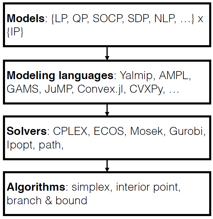
Figure 2 illustrates the typical sequence of formulating, implementing and solving optimization problems as commonly applied to engineering problems. First, a mathematical model of the optimization problem is formulated. The problem is formulated so that it can be handled by the chosen modeling language and optimization solver. Eventually, the modeling toolbox translates the mathematical model into the appropriate form for the solver interface, fills out parameter values, and dispatches the optimization solver. Finally, the mathematical solver uses one or a variety of different algorithms to solve the optimization problem, and returns a solution.
Refer to caption
Figure 2: Formulation, implementation and solution of optimization problems.

In the literature, real-value formulations of the convex relaxations of unbalanced OPF are rarely discussed. CVX has been used as an optimization modeling tool in [11]. It is one of the very few optimization packages with support for complex optimization variable primitives, as well as matrix variables. CVX automates the reformulation process from a complex-value matrix to a set of real-value scalar variables and constraints. Functionality to automate the real-value reformulation process was initially in a JuMP extension [22], but has recently become a built-in JuMP feature [23].

Gilbert and Josz [24] illustrate with a limited-scope solver that there are potential advantages of solving SDP problems directly in the complex domain. Nevertheless, a mature implementation of such a solver has not been developed so far. Overall, the interest in real-value forms remains high.

Table 6: Unbalanced power flow formulations, key references and variable spaces
Formulation Ref. Variable space Exact? Section
NLP Kirchhoff unbalanced [1, 9] 𝐈l​i​j,𝐔i{\color[rgb]{0,0,1}\mathbf{I}_{{l}{i}{j}}},{\color[rgb]{0,0,1}\mathbf{U}_{{i}}} by definition, discussion: [25] §3
NLP BIM unbalanced scalar polar [8] diag⁡(𝐒l​i​j),𝐔i\diag({\color[rgb]{0,0,1}\mathbf{S}_{{l}{i}{j}}}),{\color[rgb]{0,0,1}\mathbf{U}_{{i}}} if 𝐔imin≠𝟎{\color[rgb]{1,0,0}\mathbf{U}_{{i}}^{\text{min}}}\neq\mathbf{0} §5
NLP BIM unbalanced scalar rect. diag⁡(𝐒l​i​j),𝐔i\diag({\color[rgb]{0,0,1}\mathbf{S}_{{l}{i}{j}}}),{\color[rgb]{0,0,1}\mathbf{U}_{{i}}} if 𝐔imin≠𝟎{\color[rgb]{1,0,0}\mathbf{U}_{{i}}^{\text{min}}}\neq\mathbf{0} §5
SDP BIM unbalanced [11, 26, 27] 𝐒l​i​j,𝐖i⪰0,𝐖i​j,𝐌⪰0{\color[rgb]{0,0,1}\mathbf{S}_{{l}{i}{j}}},{\color[rgb]{0,0,1}\mathbf{W}_{{i}}}\succeq 0,{\color[rgb]{0,0,1}\mathbf{W}_{{i}{j}}},{\color[rgb]{0,0,1}\mathbf{M}}\succeq 0 rank⁡(𝐌)=1\rank({\color[rgb]{0,0,1}\mathbf{M}})=1 §6
SDP BIM unbalanced radial [12] 𝐒l​i​j,𝐖i⪰0,𝐖i​j,𝐌i​j⪰0{\color[rgb]{0,0,1}\mathbf{S}_{{l}{i}{j}}},{\color[rgb]{0,0,1}\mathbf{W}_{{i}}}\succeq 0,{\color[rgb]{0,0,1}\mathbf{W}_{{i}{j}}},{\color[rgb]{0,0,1}\mathbf{M}_{{i}{j}}}\succeq 0 rank⁡(𝐌i​j)=1\rank({\color[rgb]{0,0,1}\mathbf{M}_{{i}{j}}})=1, only if radial §6
SDP BFM unbalanced [12] 𝐒l​i​j,𝐖i⪰0,𝐋ls⪰0,𝐌l​i​j⪰0{\color[rgb]{0,0,1}\mathbf{S}_{{l}{i}{j}}},{\color[rgb]{0,0,1}\mathbf{W}_{{i}}}\succeq 0,{\color[rgb]{0,0,1}\mathbf{L}_{{l}}^{\text{{s}}}}\succeq 0,{\color[rgb]{0,0,1}\mathbf{M}_{{l}{i}{j}}}\succeq 0 rank⁡(𝐌l​i​j)=1\rank({\color[rgb]{0,0,1}\mathbf{M}_{{l}{i}{j}}})=1, only if radial §7

1.4 Scope, Contributions and Report Structure

In summary, we observe the following gaps in the literature:

  • •

    polar and rectangular real forms in the power-voltage variable space for branches with shunts (Π\Pi-model);

  • •

    real form of the power - lifted voltage BIM and BFM SDP relaxations;

  • •

    definitions of current, power and voltage angle difference limits in both the power-voltage and power-lifted voltage variable spaces.

This work therefore provides consistent derivations of real-value formulations for variants of unbalanced optimal power flow in different variable spaces, to enable straight-forward implementation in optimization modeling toolboxes and efficient comparison on published data sets.

We limit ourselves here to the three-wire case, and note that recent works [28, 29] have explored OPF models with explicit representation of the neutral.

First, the basic relationship between the different variables and parameters is defined in §2, which builds the mathematical foundation of this report; it also contains a generalized model to represent loads and generators in the system. Section §3 provides Kirchhoff’s and Ohm’s laws in the multiconductor form. Next, §4 develops a formulation of nonlinear BFM unbalanced power flow and §5 the equivalent BIM. Furthermore, §6 derives the BIM and §7 the BFM in the lifted variable space which is the basis various convex relaxations. Moreover §8 presents the feasible sets of the derived real-value formulations and discusses implementation aspects. Finally, §9 presents the conclusions.

2 Notation and Basic Relationships

2.1 Scalar and Matrix Variables

The voltage 𝐔i{\color[rgb]{0,0,1}\mathbf{U}_{{i}}} of a bus ii is a complex value, vector variable, encapsulating variables for each conductor:

𝐔i=[Ui,aUi,bUi,c]=[Ui,amag​∠​θi,aUi,bmag​∠​θi,bUi,cmag​∠​θi,c]=𝐔imag​∠​𝚯i=[Ui,are+j​Ui,aimUi,bre+j​Ui,bimUi,cre+j​Ui,cim]=𝐔ire+j​𝐔iim\displaystyle{\color[rgb]{0,0,1}\mathbf{U}_{{i}}}=\begin{bmatrix}{\color[rgb]{0,0,1}U_{{i},{a}}}\\ {\color[rgb]{0,0,1}U_{{i},{b}}}\\ {\color[rgb]{0,0,1}U_{{i},{c}}}\end{bmatrix}=\begin{bmatrix}{\color[rgb]{0,0,0}U_{{i},{a}}^{\text{mag}}}{\color[rgb]{1,0,0}\angle}{\color[rgb]{0,0,0}\theta_{{i},{a}}}\\ {\color[rgb]{0,0,0}U_{{i},{b}}^{\text{mag}}}{\color[rgb]{1,0,0}\angle}{\color[rgb]{0,0,0}\theta_{{i},{b}}}\\ {\color[rgb]{0,0,0}U_{{i},{c}}^{\text{mag}}}{\color[rgb]{1,0,0}\angle}{\color[rgb]{0,0,0}\theta_{{i},{c}}}\end{bmatrix}={\color[rgb]{0,0,0}\mathbf{U}_{{i}}^{\text{mag}}}{\color[rgb]{1,0,0}\angle}{\color[rgb]{0,0,0}\mathbf{\Theta}_{{i}}}=\begin{bmatrix}{\color[rgb]{0,0,0}U_{{i},{a}}^{\text{re}}}+{\color[rgb]{1,0,0}j}{\color[rgb]{0,0,0}U_{{i},{a}}^{\text{im}}}\\ {\color[rgb]{0,0,0}U_{{i},{b}}^{\text{re}}}+{\color[rgb]{1,0,0}j}{\color[rgb]{0,0,0}U_{{i},{b}}^{\text{im}}}\\ {\color[rgb]{0,0,0}U_{{i},{c}}^{\text{re}}}+{\color[rgb]{1,0,0}j}{\color[rgb]{0,0,0}U_{{i},{c}}^{\text{im}}}\end{bmatrix}={\color[rgb]{0,0,0}\mathbf{U}_{{i}}^{\text{re}}}+{\color[rgb]{1,0,0}j}{\color[rgb]{0,0,0}\mathbf{U}_{{i}}^{\text{im}}} (1)

Similarly, the total current of a branch ll connecting a pair of buses ii and jj is a complex value vector variable,

𝐈l​i​j=[Il​i​j,aIl​i​j,bIl​i​j,c].\displaystyle{\color[rgb]{0,0,1}\mathbf{I}_{{l}{i}{j}}}=\begin{bmatrix}{\color[rgb]{0,0,1}I_{{l}{i}{j},{a}}}\\ {\color[rgb]{0,0,1}I_{{l}{i}{j},{b}}}\\ {\color[rgb]{0,0,1}I_{{l}{i}{j},{c}}}\end{bmatrix}.

The sending-side current (i→ji\rightarrow j) through the series element in the Π\Pi-model is defined as 𝐈l​i​js{\color[rgb]{0,0,1}\mathbf{I}_{{l}{i}{j}}^{\text{{s}}}}, the sending-side shunt current as 𝐈l​i​jsh{\color[rgb]{0,0,1}\mathbf{I}_{{l}{i}{j}}^{\text{{sh}}}}, respectively. The complex power flow in branch ll from bus i{i} to j{j} depends on the bus voltage of the sending-side 𝐔i{\color[rgb]{0,0,1}\mathbf{U}_{{i}}} and the conjugate transpose (indicated with superscript H) of the current 𝐈l​i​j{\color[rgb]{0,0,1}\mathbf{I}_{{l}{i}{j}}},

𝐒l​i​j=𝐔i​(𝐈l​i​j)H=[Sl​i​j,a​aSl​i​j,a​bSl​i​j,a​cSl​i​j,b​aSl​i​j,b​bSl​i​j,b​cSl​i​j,c​aSl​i​j,c​bSl​i​j,c​c].\displaystyle{\color[rgb]{0,0,1}\mathbf{S}_{{l}{i}{j}}}={\color[rgb]{0,0,1}\mathbf{U}_{{i}}}({\color[rgb]{0,0,1}\mathbf{I}_{{l}{i}{j}}})^{\text{H}}=\left[\begin{array}[]{ccc}{\color[rgb]{0,0,1}S_{{l}{i}{j},{a}{a}}}&{\color[rgb]{0,0,1}S_{{l}{i}{j},{a}{b}}}&{\color[rgb]{0,0,1}S_{{l}{i}{j},{a}{c}}}\\ {\color[rgb]{0,0,1}S_{{l}{i}{j},{b}{a}}}&{\color[rgb]{0,0,1}S_{{l}{i}{j},{b}{b}}}&{\color[rgb]{0,0,1}S_{{l}{i}{j},{b}{c}}}\\ {\color[rgb]{0,0,1}S_{{l}{i}{j},{c}{a}}}&{\color[rgb]{0,0,1}S_{{l}{i}{j},{c}{b}}}&{\color[rgb]{0,0,1}S_{{l}{i}{j},{c}{c}}}\end{array}\right].

We observe that diag⁡(𝐒l​i​j)=𝐔i∘(𝐈l​i​j)∗\diag({\color[rgb]{0,0,1}\mathbf{S}_{{l}{i}{j}}})={\color[rgb]{0,0,1}\mathbf{U}_{{i}}}\circ({\color[rgb]{0,0,1}\mathbf{I}_{{l}{i}{j}}})^{*}, where ∘\circ is the element-wise (Hadamard) product. It is noted that rank⁡(𝐒l​i​j)=1\rank({\color[rgb]{0,0,1}\mathbf{S}_{{l}{i}{j}}})=1, as it is defined as the outer product of two vectors. The off-diagonals relate to the diagonal elements according to,

Sl​i​j,a​aUi,a=Sl​i​j,b​aUi,b=Sl​i​j,c​aUi,c=(Il​i​j,a)∗,\displaystyle\frac{{\color[rgb]{0,0,1}S_{{l}{i}{j},{a}{a}}}}{{\color[rgb]{0,0,1}U_{{i},{a}}}}=\frac{{\color[rgb]{0,0,1}S_{{l}{i}{j},{b}{a}}}}{{\color[rgb]{0,0,1}U_{{i},{b}}}}=\frac{{\color[rgb]{0,0,1}S_{{l}{i}{j},{c}{a}}}}{{\color[rgb]{0,0,1}U_{{i},{c}}}}=({\color[rgb]{0,0,1}I_{{l}{i}{j},{a}}})^{*}, (6a)
Sl​i​j,b​bUi,b=Sl​i​j,a​bUi,a=Sl​i​j,c​bUi,c=(Il​i​j,b)∗,\displaystyle\frac{{\color[rgb]{0,0,1}S_{{l}{i}{j},{b}{b}}}}{{\color[rgb]{0,0,1}U_{{i},{b}}}}=\frac{{\color[rgb]{0,0,1}S_{{l}{i}{j},{a}{b}}}}{{\color[rgb]{0,0,1}U_{{i},{a}}}}=\frac{{\color[rgb]{0,0,1}S_{{l}{i}{j},{c}{b}}}}{{\color[rgb]{0,0,1}U_{{i},{c}}}}=({\color[rgb]{0,0,1}I_{{l}{i}{j},{b}}})^{*}, (7a)
Sl​i​j,c​cUi,c=Sl​i​j,a​cUi,a=Sl​i​j,b​cUi,b=(Il​i​j,c)∗,\displaystyle\frac{{\color[rgb]{0,0,1}S_{{l}{i}{j},{c}{c}}}}{{\color[rgb]{0,0,1}U_{{i},{c}}}}=\frac{{\color[rgb]{0,0,1}S_{{l}{i}{j},{a}{c}}}}{{\color[rgb]{0,0,1}U_{{i},{a}}}}=\frac{{\color[rgb]{0,0,1}S_{{l}{i}{j},{b}{c}}}}{{\color[rgb]{0,0,1}U_{{i},{b}}}}=({\color[rgb]{0,0,1}I_{{l}{i}{j},{c}}})^{*}, (8a)

which means that the off-diagonals of 𝐒l​i​j{\color[rgb]{0,0,1}\mathbf{S}_{{l}{i}{j}}} are scaled and rotated versions of the more easily interpretable diagonal elements.

2.2 Variable Bounds

Voltage magnitudes have minimum and maximum operational limits, which are specific to each bus and phase,

𝟎≤[Ui,aminUi,bminUi,cmin]⏟𝐔imin≤[|Ui,a||Ui,b||Ui,c|]≤[Ui,amaxUi,bmaxUi,cmax]⏟𝐔imax.\displaystyle\mathbf{0}\leq\underbrace{\begin{bmatrix}{\color[rgb]{1,0,0}U_{{i},{a}}^{\text{min}}}\\ {\color[rgb]{1,0,0}U_{{i},{b}}^{\text{min}}}\\ {\color[rgb]{1,0,0}U_{{i},{c}}^{\text{min}}}\\ \end{bmatrix}}_{{\color[rgb]{1,0,0}\mathbf{U}_{{i}}^{\text{min}}}}\leq\begin{bmatrix}|{\color[rgb]{0,0,1}U_{{i},{a}}}|\\ |{\color[rgb]{0,0,1}U_{{i},{b}}}|\\ |{\color[rgb]{0,0,1}U_{{i},{c}}}|\\ \end{bmatrix}\leq\underbrace{\begin{bmatrix}{\color[rgb]{1,0,0}U_{{i},{a}}^{\text{max}}}\\ {\color[rgb]{1,0,0}U_{{i},{b}}^{\text{max}}}\\ {\color[rgb]{1,0,0}U_{{i},{c}}^{\text{max}}}\\ \end{bmatrix}}_{{\color[rgb]{1,0,0}\mathbf{U}_{{i}}^{\text{max}}}}. (9)

In this report, we overload ‘≤\leq’ for ‘≥\geq’ for vectors and matrices to indicate element-wise inequality (conversely, ‘⪰\succeq’ is used as the symbol for matrix positive semidefiniteness). Recognizing we obtain the magnitude squared by multiplying complex numbers with their own conjugates, the nodal voltage bounds can also be presented quadratically as:

𝟎≤𝐔imin∘𝐔imin≤𝐔i∘(𝐔i)∗≤𝐔imax∘𝐔imax.\displaystyle\mathbf{0}\leq{\color[rgb]{1,0,0}\mathbf{U}_{{i}}^{\text{min}}}\circ{\color[rgb]{1,0,0}\mathbf{U}_{{i}}^{\text{min}}}\leq{\color[rgb]{0,0,1}\mathbf{U}_{{i}}}\circ({\color[rgb]{0,0,1}\mathbf{U}_{{i}}})^{*}\leq{\color[rgb]{1,0,0}\mathbf{U}_{{i}}^{\text{max}}}\circ{\color[rgb]{1,0,0}\mathbf{U}_{{i}}^{\text{max}}}. (10)

Note that the upper bound constraints are convex (space inside a circle), but the lower bound constraints are nonconvex (space outside of a circle). Next, apparent power limits are defined using the absolute value of the diagonals of the branch flow matrix,

𝟎≤[|Sl​i​j,a​a||Sl​i​j,b​b||Sl​i​j,c​c|]≤[Sl​i​j,aratedSl​i​j,bratedSl​i​j,crated]=𝐒l​i​jrated,\displaystyle\mathbf{0}\leq\begin{bmatrix}|{\color[rgb]{0,0,1}S_{{l}{i}{j},{a}{a}}}|\\ |{\color[rgb]{0,0,1}S_{{l}{i}{j},{b}{b}}}|\\ |{\color[rgb]{0,0,1}S_{{l}{i}{j},{c}{c}}}|\\ \end{bmatrix}\leq\begin{bmatrix}{\color[rgb]{1,0,0}S_{{l}{i}{j},{a}}^{\text{rated}}}\\ {\color[rgb]{1,0,0}S_{{l}{i}{j},{b}}^{\text{rated}}}\\ {\color[rgb]{1,0,0}S_{{l}{i}{j},{c}}^{\text{rated}}}\\ \end{bmatrix}={\color[rgb]{1,0,0}\mathbf{S}_{{l}{i}{j}}^{\text{rated}}}, (11)

which is equivalent to second order cone (SOC) constraints,

[|Sl​i​j,a​a|2|Sl​i​j,b​b|2|Sl​i​j,c​c|2]=[(Pl​i​j,a​a)2+(Ql​i​j,a​a)2(Pl​i​j,b​b)2+(Ql​i​j,b​b)2(Pl​i​j,c​c)2+(Ql​i​j,c​c)2]≤[(Sl​i​j,arated)2(Sl​i​j,brated)2(Sl​i​j,crated)2],\displaystyle\begin{bmatrix}|{\color[rgb]{0,0,1}S_{{l}{i}{j},{a}{a}}}|^{2}\\ |{\color[rgb]{0,0,1}S_{{l}{i}{j},{b}{b}}}|^{2}\\ |{\color[rgb]{0,0,1}S_{{l}{i}{j},{c}{c}}}|^{2}\\ \end{bmatrix}=\begin{bmatrix}({\color[rgb]{0,0,0}P_{{l}{i}{j},{a}{a}}})^{2}+({\color[rgb]{0,0,0}Q_{{l}{i}{j},{a}{a}}})^{2}\\ ({\color[rgb]{0,0,0}P_{{l}{i}{j},{b}{b}}})^{2}+({\color[rgb]{0,0,0}Q_{{l}{i}{j},{b}{b}}})^{2}\\ ({\color[rgb]{0,0,0}P_{{l}{i}{j},{c}{c}}})^{2}+({\color[rgb]{0,0,0}Q_{{l}{i}{j},{c}{c}}})^{2}\\ \end{bmatrix}\leq\begin{bmatrix}({\color[rgb]{1,0,0}S_{{l}{i}{j},{a}}^{\text{rated}}})^{2}\\ ({\color[rgb]{1,0,0}S_{{l}{i}{j},{b}}^{\text{rated}}})^{2}\\ ({\color[rgb]{1,0,0}S_{{l}{i}{j},{c}}^{\text{rated}}})^{2}\\ \end{bmatrix}, (12)

and can succinctly be written as,

𝟎≤diag⁡(𝐒l​i​j)∘diag⁡(𝐒l​i​j)∗≤𝐒l​i​jrated∘𝐒l​i​jrated.\displaystyle\mathbf{0}\leq\diag({\color[rgb]{0,0,1}\mathbf{S}_{{l}{i}{j}}})\circ\diag({\color[rgb]{0,0,1}\mathbf{S}_{{l}{i}{j}}})^{*}\leq{\color[rgb]{1,0,0}\mathbf{S}_{{l}{i}{j}}^{\text{rated}}}\circ{\color[rgb]{1,0,0}\mathbf{S}_{{l}{i}{j}}^{\text{rated}}}. (13)

The magnitudes of the branch current should stay below rated values and are bounded for the diagonals of the branch current matrix,

𝟎≤[|Il​i​j,a||Il​i​j,b||Il​i​j,c|]≤[Il​i​j,aratedIl​i​j,bratedIl​i​j,crated]=𝐈l​i​jrated,\displaystyle\mathbf{0}\leq\begin{bmatrix}|{\color[rgb]{0,0,1}I_{{l}{i}{j},{a}}}|\\ |{\color[rgb]{0,0,1}I_{{l}{i}{j},{b}}}|\\ |{\color[rgb]{0,0,1}I_{{l}{i}{j},{c}}}|\\ \end{bmatrix}\leq\begin{bmatrix}{\color[rgb]{1,0,0}I_{{l}{i}{j},{a}}^{\text{rated}}}\\ {\color[rgb]{1,0,0}I_{{l}{i}{j},{b}}^{\text{rated}}}\\ {\color[rgb]{1,0,0}I_{{l}{i}{j},{c}}^{\text{rated}}}\\ \end{bmatrix}={\color[rgb]{1,0,0}\mathbf{I}_{{l}{i}{j}}^{\text{rated}}}, (14)

which again can be written as a set of SOC constraints,

𝟎≤𝐈l​i​j∘(𝐈l​i​j)∗≤𝐈l​i​jrated∘𝐈l​i​jrated.\displaystyle\mathbf{0}\leq{\color[rgb]{0,0,1}\mathbf{I}_{{l}{i}{j}}}\circ({\color[rgb]{0,0,1}\mathbf{I}_{{l}{i}{j}}})^{*}\leq{\color[rgb]{1,0,0}\mathbf{I}_{{l}{i}{j}}^{\text{rated}}}\circ{\color[rgb]{1,0,0}\mathbf{I}_{{l}{i}{j}}^{\text{rated}}}. (15)

A valid SOC representation of current magnitude limits (14) that does not require explicit current variables 𝐈l​i​j{\color[rgb]{0,0,1}\mathbf{I}_{{l}{i}{j}}} is useful for BIM forms. Using the nodal voltage magnitudes, the branch current limits can directly be enforced on the power flows,

[|Sl​i​j,a​a|2|Sl​i​j,b​b|2|Sl​i​j,c​c|2]≤[(Il​i​j,arated)2(Il​i​j,brated)2(Il​i​j,crated)2]∘[|Ui,a|2|Ui,b|2|Ui,c|2],\displaystyle\begin{bmatrix}|{\color[rgb]{0,0,1}S_{{l}{i}{j},{a}{a}}}|^{2}\\ |{\color[rgb]{0,0,1}S_{{l}{i}{j},{b}{b}}}|^{2}\\ |{\color[rgb]{0,0,1}S_{{l}{i}{j},{c}{c}}}|^{2}\\ \end{bmatrix}\leq\begin{bmatrix}({\color[rgb]{1,0,0}I_{{l}{i}{j},{a}}^{\text{rated}}})^{2}\\ ({\color[rgb]{1,0,0}I_{{l}{i}{j},{b}}^{\text{rated}}})^{2}\\ ({\color[rgb]{1,0,0}I_{{l}{i}{j},{c}}^{\text{rated}}})^{2}\\ \end{bmatrix}\circ\begin{bmatrix}|{\color[rgb]{0,0,1}U_{{i},{a}}}|^{2}\\ |{\color[rgb]{0,0,1}U_{{i},{b}}}|^{2}\\ |{\color[rgb]{0,0,1}U_{{i},{c}}}|^{2}\\ \end{bmatrix}, (16)

which can also be developed in matrix notation as,

diag⁡(𝐒l​i​j)∘diag⁡(𝐒l​i​j)∗≤𝐈l​i​jrated∘𝐈l​i​jrated∘𝐔i∘(𝐔i)∗.\displaystyle\diag({\color[rgb]{0,0,1}\mathbf{S}_{{l}{i}{j}}})\circ\diag({\color[rgb]{0,0,1}\mathbf{S}_{{l}{i}{j}}})^{*}\leq{\color[rgb]{1,0,0}\mathbf{I}_{{l}{i}{j}}^{\text{rated}}}\circ{\color[rgb]{1,0,0}\mathbf{I}_{{l}{i}{j}}^{\text{rated}}}\circ{\color[rgb]{0,0,1}\mathbf{U}_{{i}}}\circ({\color[rgb]{0,0,1}\mathbf{U}_{{i}}})^{*}. (17)

Valid bounds on all elements of the power flow matrix 𝐒l​i​j=𝐏l​i​j+j​𝐐l​i​j{\color[rgb]{0,0,1}\mathbf{S}_{{l}{i}{j}}}={\color[rgb]{0,0,0}\mathbf{P}_{{l}{i}{j}}}+{\color[rgb]{1,0,0}j}{\color[rgb]{0,0,0}\mathbf{Q}_{{l}{i}{j}}} are,

−𝐔imax​(𝐈l​i​jrated)T≤𝐏l​i​j,𝐐l​i​j≤𝐔imax​(𝐈l​i​jrated)T,\displaystyle-{\color[rgb]{1,0,0}\mathbf{U}_{{i}}^{\text{max}}}({\color[rgb]{1,0,0}\mathbf{I}_{{l}{i}{j}}^{\text{rated}}})^{\text{T}}\leq{\color[rgb]{0,0,0}\mathbf{P}_{{l}{i}{j}}},{\color[rgb]{0,0,0}\mathbf{Q}_{{l}{i}{j}}}\leq{\color[rgb]{1,0,0}\mathbf{U}_{{i}}^{\text{max}}}({\color[rgb]{1,0,0}\mathbf{I}_{{l}{i}{j}}^{\text{rated}}})^{\text{T}}, (18)

both for active and reactive power components, respectively. The voltage angle differences between connected buses ii and jj are bounded,

[−π2−π2−π2]≤[θi​j,a​aminθi​j,b​bminθi​j,c​cmin]⏟𝚯i​jmin≤[θi,a−θj,aθi,b−θj,bθi,c−θj,c]≤[θi​j,a​amaxθi​j,b​bmaxθi​j,c​cmax]⏟𝚯i​jmax≤[π2π2π2].\displaystyle\!\begin{bmatrix}-\frac{\pi}{2}\\ -\frac{\pi}{2}\\ -\frac{\pi}{2}\end{bmatrix}\leq\underbrace{\begin{bmatrix}{\color[rgb]{1,0,0}\theta_{{i}{j},{a}{a}}^{\text{min}}}\\ {\color[rgb]{1,0,0}\theta_{{i}{j},{b}{b}}^{\text{min}}}\\ {\color[rgb]{1,0,0}\theta_{{i}{j},{c}{c}}^{\text{min}}}\end{bmatrix}}_{{\color[rgb]{1,0,0}\mathbf{\Theta}_{{i}{j}}^{\text{min}}}}\leq\begin{bmatrix}{\color[rgb]{0,0,0}\theta_{{i},{a}}}-{\color[rgb]{0,0,0}\theta_{{j},{a}}}\\ {\color[rgb]{0,0,0}\theta_{{i},{b}}}-{\color[rgb]{0,0,0}\theta_{{j},{b}}}\\ {\color[rgb]{0,0,0}\theta_{{i},{c}}}-{\color[rgb]{0,0,0}\theta_{{j},{c}}}\end{bmatrix}\leq\underbrace{\begin{bmatrix}{\color[rgb]{1,0,0}\theta_{{i}{j},{a}{a}}^{\text{max}}}\\ {\color[rgb]{1,0,0}\theta_{{i}{j},{b}{b}}^{\text{max}}}\\ {\color[rgb]{1,0,0}\theta_{{i}{j},{c}{c}}^{\text{max}}}\end{bmatrix}}_{{\color[rgb]{1,0,0}\mathbf{\Theta}_{{i}{j}}^{\text{max}}}}\leq\begin{bmatrix}\frac{\pi}{2}\\ \frac{\pi}{2}\\ \frac{\pi}{2}\end{bmatrix}. (19)

For a relatively balanced voltage phasor, we expect θi,a−θi,b≈θi,b−θi,c≈θi,c−θi,a≈2​π3{\color[rgb]{0,0,0}\theta_{{i},{a}}}-{\color[rgb]{0,0,0}\theta_{{i},{b}}}\approx{\color[rgb]{0,0,0}\theta_{{i},{b}}}-{\color[rgb]{0,0,0}\theta_{{i},{c}}}\approx{\color[rgb]{0,0,0}\theta_{{i},{c}}}-{\color[rgb]{0,0,0}\theta_{{i},{a}}}\approx\frac{2\pi}{3}. The voltage angle differences between phases on buses ii can be bounded to enforce angle balance relative to the expected 120 degrees,

[θi,a​aminθi,b​bminθi,c​cmin]⏟𝚯imin≤[θi,a−θi,b−2​π3θi,b−θi,c−2​π3θi,c−θi,a−2​π3]≤[θi,a​amaxθi,b​bmaxθi,c​cmax]⏟𝚯imax.\displaystyle\underbrace{\begin{bmatrix}{\color[rgb]{1,0,0}\theta_{{i},{a}{a}}^{\text{min}}}\\ {\color[rgb]{1,0,0}\theta_{{i},{b}{b}}^{\text{min}}}\\ {\color[rgb]{1,0,0}\theta_{{i},{c}{c}}^{\text{min}}}\end{bmatrix}}_{{\color[rgb]{1,0,0}\mathbf{\Theta}_{{i}}^{\text{min}}}}\leq\begin{bmatrix}{\color[rgb]{0,0,0}\theta_{{i},{a}}}-{\color[rgb]{0,0,0}\theta_{{i},{b}}}-\frac{2\pi}{3}\\ {\color[rgb]{0,0,0}\theta_{{i},{b}}}-{\color[rgb]{0,0,0}\theta_{{i},{c}}}-\frac{2\pi}{3}\\ {\color[rgb]{0,0,0}\theta_{{i},{c}}}-{\color[rgb]{0,0,0}\theta_{{i},{a}}}-\frac{2\pi}{3}\end{bmatrix}\leq\underbrace{\begin{bmatrix}{\color[rgb]{1,0,0}\theta_{{i},{a}{a}}^{\text{max}}}\\ {\color[rgb]{1,0,0}\theta_{{i},{b}{b}}^{\text{max}}}\\ {\color[rgb]{1,0,0}\theta_{{i},{c}{c}}^{\text{max}}}\end{bmatrix}}_{{\color[rgb]{1,0,0}\mathbf{\Theta}_{{i}}^{\text{max}}}}. (20)

The voltage phasor in reference buses i∈ℐref⊂ℐi\in{\color[rgb]{1,0,0}\mathcal{I}}_{\text{ref}}\subset{\color[rgb]{1,0,0}\mathcal{I}} is assumed fixed, e.g.,

𝐔i=𝐔iref=[Ui,aref​∠​θi,arefUi,bref​∠​θi,brefUi,cref​∠​θi,cref].\displaystyle{\color[rgb]{0,0,1}\mathbf{U}_{{i}}}={\color[rgb]{0.75,0.5,0.25}\mathbf{U}_{{i}}^{\text{ref}}}=\begin{bmatrix}{\color[rgb]{1,0,0}U_{{i},{a}}^{\text{ref}}}{\color[rgb]{1,0,0}\angle}{\color[rgb]{1,0,0}\theta_{{i},{a}}^{\text{ref}}}\\ {\color[rgb]{1,0,0}U_{{i},{b}}^{\text{ref}}}{\color[rgb]{1,0,0}\angle}{\color[rgb]{1,0,0}\theta_{{i},{b}}^{\text{ref}}}\\ {\color[rgb]{1,0,0}U_{{i},{c}}^{\text{ref}}}{\color[rgb]{1,0,0}\angle}{\color[rgb]{1,0,0}\theta_{{i},{c}}^{\text{ref}}}\end{bmatrix}. (21)

2.3 Branch Impedance

The circuit series impedance matrix is defined as a full matrix with no assumption on the particular structure:

𝐳ls=𝐫ls+j​𝐱ls=[zl,a​aszl,a​bszl,a​cszl,b​aszl,b​bszl,b​cszl,c​aszl,c​bszl,c​cs],\displaystyle{\color[rgb]{0.75,0.5,0.25}\mathbf{z}_{{l}}^{\text{{s}}}}={\color[rgb]{1,0,0}\mathbf{r}_{{l}}^{\text{{s}}}}+{\color[rgb]{1,0,0}j}{\color[rgb]{1,0,0}\mathbf{x}_{{l}}^{\text{{s}}}}=\begin{bmatrix}{\color[rgb]{0.75,0.5,0.25}z_{{l},{a}{a}}^{\text{{s}}}}&{\color[rgb]{0.75,0.5,0.25}z_{{l},{a}{b}}^{\text{{s}}}}&{\color[rgb]{0.75,0.5,0.25}z_{{l},{a}{c}}^{\text{{s}}}}\\ {\color[rgb]{0.75,0.5,0.25}z_{{l},{b}{a}}^{\text{{s}}}}&{\color[rgb]{0.75,0.5,0.25}z_{{l},{b}{b}}^{\text{{s}}}}&{\color[rgb]{0.75,0.5,0.25}z_{{l},{b}{c}}^{\text{{s}}}}\\ {\color[rgb]{0.75,0.5,0.25}z_{{l},{c}{a}}^{\text{{s}}}}&{\color[rgb]{0.75,0.5,0.25}z_{{l},{c}{b}}^{\text{{s}}}}&{\color[rgb]{0.75,0.5,0.25}z_{{l},{c}{c}}^{\text{{s}}}}\\ \end{bmatrix}, (22)

where each element consists of a series resistive and reactive impedance. It is noted that in physical systems, we expect 𝐫ls⪰0,𝐱ls⪰0{\color[rgb]{1,0,0}\mathbf{r}_{{l}}^{\text{{s}}}}\succeq 0,{\color[rgb]{1,0,0}\mathbf{x}_{{l}}^{\text{{s}}}}\succeq 0. The impedance matrix can be rewritten in the corresponding admittance form,

𝐲ls=(𝐳ls)−1=𝐠ls+j​𝐛ls.\displaystyle{\color[rgb]{0.75,0.5,0.25}\mathbf{y}_{{l}}^{\text{{s}}}}={({\color[rgb]{0.75,0.5,0.25}\mathbf{z}_{{l}}^{\text{{s}}}})^{-1}}={\color[rgb]{1,0,0}\mathbf{g}_{{l}}^{\text{{s}}}}+{\color[rgb]{1,0,0}j}{\color[rgb]{1,0,0}\mathbf{b}_{{l}}^{\text{{s}}}}.

where (𝐳ls)−1{({\color[rgb]{0.75,0.5,0.25}\mathbf{z}_{{l}}^{\text{{s}}}})^{-1}} is the matrix inverse of 𝐳ls{\color[rgb]{0.75,0.5,0.25}\mathbf{z}_{{l}}^{\text{{s}}}}. In case of missing conductors, e.g. single, or two-conductor connections, 𝐳ls{\color[rgb]{0.75,0.5,0.25}\mathbf{z}_{{l}}^{\text{{s}}}} is not invertible but it is valid to use the Moore-Penrose inverse instead. The shunt admittances at the sending and receiving sides, respectively 𝐲l​i​jsh,𝐲l​j​ish{\color[rgb]{0.75,0.5,0.25}\mathbf{y}_{{l}{i}{j}}^{\text{{sh}}}},{\color[rgb]{0.75,0.5,0.25}\mathbf{y}_{{l}{j}{i}}^{\text{{sh}}}}, are defined,

𝐲l​i​jsh=𝐠l​i​jsh+j​𝐛l​i​jsh=[yl​i​j,a​ashyl​i​j,a​bshyl​i​j,a​cshyl​i​j,b​ashyl​i​j,b​bshyl​i​j,b​cshyl​i​j,c​ashyl​i​j,c​bshyl​i​j,c​csh].\displaystyle{\color[rgb]{0.75,0.5,0.25}\mathbf{y}_{{l}{i}{j}}^{\text{{sh}}}}={\color[rgb]{1,0,0}\mathbf{g}_{{l}{i}{j}}^{\text{{sh}}}}+{\color[rgb]{1,0,0}j}{\color[rgb]{1,0,0}\mathbf{b}_{{l}{i}{j}}^{\text{{sh}}}}=\begin{bmatrix}{\color[rgb]{0.75,0.5,0.25}y_{{l}{i}{j},{a}{a}}^{\text{{sh}}}}&{\color[rgb]{0.75,0.5,0.25}y_{{l}{i}{j},{a}{b}}^{\text{{sh}}}}&{\color[rgb]{0.75,0.5,0.25}y_{{l}{i}{j},{a}{c}}^{\text{{sh}}}}\\ {\color[rgb]{0.75,0.5,0.25}y_{{l}{i}{j},{b}{a}}^{\text{{sh}}}}&{\color[rgb]{0.75,0.5,0.25}y_{{l}{i}{j},{b}{b}}^{\text{{sh}}}}&{\color[rgb]{0.75,0.5,0.25}y_{{l}{i}{j},{b}{c}}^{\text{{sh}}}}\\ {\color[rgb]{0.75,0.5,0.25}y_{{l}{i}{j},{c}{a}}^{\text{{sh}}}}&{\color[rgb]{0.75,0.5,0.25}y_{{l}{i}{j},{c}{b}}^{\text{{sh}}}}&{\color[rgb]{0.75,0.5,0.25}y_{{l}{i}{j},{c}{c}}^{\text{{sh}}}}\\ \end{bmatrix}. (23)

Although for typical distribution lines and cables the shunt admittances are diagonal and have equal values for both sides, in this generalized derivation they can be considered as a two different and full matrices. This also allows for re-use of the representation for other elements, such as transformers.

2.4 Loads and Generators as Units

We define units u∈𝒰{u}\in{\color[rgb]{1,0,0}\mathcal{U}} to generalize loads, generators and storage elements. The current flowing from the connected bus into the unit is

𝐈u=[Iu,aIu,bIu,c].\displaystyle{\color[rgb]{0,0,1}\mathbf{I}_{{u}}}=\begin{bmatrix}{\color[rgb]{0,0,1}{I}_{{u},{a}}}\\ {\color[rgb]{0,0,1}{I}_{{u},{b}}}\\ {\color[rgb]{0,0,1}{I}_{{u},{c}}}\\ \end{bmatrix}. (24)

The unit current is bounded by the corresponding current rating 𝐈urated{\color[rgb]{1,0,0}\mathbf{I}_{{u}}^{\text{rated}}} similarly to (14). Tuples of units and the buses they are connected to are defined in the connectivity set u​i∈𝒯units{u}{i}\in{\color[rgb]{1,0,0}\mathcal{T^{\text{units}}}}. The active and reactive power consumed by a unit is defined 𝐒u=𝐏u+j​𝐐u=𝐔i​(𝐈u)H{\color[rgb]{0,0,1}\mathbf{S}_{{u}}}={\color[rgb]{0,0,0}\mathbf{P}_{{u}}}+{\color[rgb]{1,0,0}j}{\color[rgb]{0,0,0}\mathbf{Q}_{{u}}}={\color[rgb]{0,0,1}\mathbf{U}_{{i}}}({\color[rgb]{0,0,1}\mathbf{I}_{{u}}})^{\text{H}}. We define bounds on active/reactive power dispatch separately,

𝐏umin≤diag⁡(𝐏u)≤𝐏umax,\displaystyle{\color[rgb]{1,0,0}\mathbf{P}_{{u}}^{\text{min}}}\leq\diag({\color[rgb]{0,0,0}\mathbf{P}_{{u}}})\leq{\color[rgb]{1,0,0}\mathbf{P}_{{u}}^{\text{max}}}, (25a)
𝐐umin≤diag⁡(𝐐u)≤𝐐umax.\displaystyle{\color[rgb]{1,0,0}\mathbf{Q}_{{u}}^{\text{min}}}\leq\diag({\color[rgb]{0,0,0}\mathbf{Q}_{{u}}})\leq{\color[rgb]{1,0,0}\mathbf{Q}_{{u}}^{\text{max}}}. (26a)

We do not provide any further detail on the specific modeling of delta or wye-connected units and refer to [13, 17].

2.5 Shunts

A shunt element, e.g. shunt capacitance, inductance or resistance, with index h{h} has an admittance 𝐲h=𝐠h+j​𝐛h{\color[rgb]{0.75,0.5,0.25}\mathbf{y}_{{h}}}={\color[rgb]{1,0,0}\mathbf{g}_{{h}}}+{\color[rgb]{1,0,0}j}{\color[rgb]{1,0,0}\mathbf{b}_{{h}}}. Tuples of shunts and the bus they are connected to are defined in the connectivity set h​i∈𝒯shunts{h}{i}\in{\color[rgb]{1,0,0}\mathcal{T^{\text{shunts}}}} . The current from the bus to the shunt is,

𝐈h=[Ih,aIh,bIh,c].\displaystyle{\color[rgb]{0,0,1}\mathbf{I}_{{h}}}=\begin{bmatrix}{\color[rgb]{0,0,1}{I}_{{h},{a}}}\\ {\color[rgb]{0,0,1}{I}_{{h},{b}}}\\ {\color[rgb]{0,0,1}{I}_{{h},{c}}}\\ \end{bmatrix}. (27)

and is bounded by the rated current 𝐈hrated{\color[rgb]{1,0,0}\mathbf{I}_{{h}}^{\text{rated}}}.

3 Application of Circuit Laws

This section illustrates how Kirchhoff’s and Ohm’s laws are used in the context of multi-conductor branches with matrix impedances for the representation of the circuit physics, providing the relationship between the voltage, current and power variables.

3.1 Branch Model

Ohm’s law for branch l​i​jlij representing the voltage drop along the branch is formulated in matrix form using nodal voltages, the branch current and the impedance matrix,

𝐔j=𝐔i−𝐳ls​𝐈l​i​js.\displaystyle{\color[rgb]{0,0,1}\mathbf{U}_{{j}}}={\color[rgb]{0,0,1}\mathbf{U}_{{i}}}-{\color[rgb]{0.75,0.5,0.25}\mathbf{z}_{{l}}^{\text{{s}}}}{\color[rgb]{0,0,1}\mathbf{I}_{{l}{i}{j}}^{\text{{s}}}}. (28)

Kirchhoff’s current law (KCL) is used to split up the series and shunt (to ground) currents in the Π\Pi-section,

𝐈l​i​j=𝐈l​i​js+𝐈l​i​jsh,𝐈l​j​i=𝐈l​j​is+𝐈l​j​ish,\displaystyle{\color[rgb]{0,0,1}\mathbf{I}_{{l}{i}{j}}}={\color[rgb]{0,0,1}\mathbf{I}_{{l}{i}{j}}^{\text{{s}}}}+{\color[rgb]{0,0,1}\mathbf{I}_{{l}{i}{j}}^{\text{{sh}}}},{\color[rgb]{0,0,1}\mathbf{I}_{{l}{j}{i}}}={\color[rgb]{0,0,1}\mathbf{I}_{{l}{j}{i}}^{\text{{s}}}}+{\color[rgb]{0,0,1}\mathbf{I}_{{l}{j}{i}}^{\text{{sh}}}}, (29)
𝐈l​i​js+𝐈l​j​is=0.\displaystyle{\color[rgb]{0,0,1}\mathbf{I}_{{l}{i}{j}}^{\text{{s}}}}+{\color[rgb]{0,0,1}\mathbf{I}_{{l}{j}{i}}^{\text{{s}}}}=0. (30)

Fig. 3 defines the harmonized single-wire equivalent vector/matrix variables in both natural and lifted (defined in upcoming sections) variable spaces for a clear presentation of the basic relationships. The scalar representation of all variables and parameters is defined in Fig. 1.

Figure 3: Power flow and losses in unbalanced Π\Pi-model branch

3.2 Shunts and Units at Nodes

The unit model can be adapted for a variety of optimization problems, e.g. optimal dispatch of distributed generation, optimal scheduling of storage and electric vehicle charging and optimal demand management. Such extensions essentially define feasible sets dependent on diag⁡(𝐏u),diag⁡(𝐐u)\diag({\color[rgb]{0,0,0}\mathbf{P}_{{u}}}),\diag({\color[rgb]{0,0,0}\mathbf{Q}_{{u}}}). Without loss of generality, in this work, we focus on the feasible sets defined by (25a)-(26a).

Similarly, the shunt power 𝐒h{\color[rgb]{0,0,1}\mathbf{S}_{{h}}} is defined as

𝐒h=𝐏h+j​𝐐h=𝐔i​(𝐈h)H.\displaystyle{\color[rgb]{0,0,1}\mathbf{S}_{{h}}}={\color[rgb]{0,0,0}\mathbf{P}_{{h}}}+{\color[rgb]{1,0,0}j}{\color[rgb]{0,0,0}\mathbf{Q}_{{h}}}={\color[rgb]{0,0,1}\mathbf{U}_{{i}}}({\color[rgb]{0,0,1}\mathbf{I}_{{h}}})^{\text{H}}. (31)

The shunt current relates to the voltage through Ohm’s law,

𝐈h=𝐲h​𝐔i.\displaystyle{\color[rgb]{0,0,1}\mathbf{I}_{{h}}}={\color[rgb]{0.75,0.5,0.25}\mathbf{y}_{{h}}}{\color[rgb]{0,0,1}\mathbf{U}_{{i}}}. (32)

Substituting (32) into (31), the shunt power consumption can be expressed depending on the nodal voltage only,

𝐒h=𝐔i​(𝐔i)H​(𝐲h)H.\displaystyle{\color[rgb]{0,0,1}\mathbf{S}_{{h}}}={\color[rgb]{0,0,1}\mathbf{U}_{{i}}}({\color[rgb]{0,0,1}\mathbf{U}_{{i}}})^{\text{H}}({\color[rgb]{0.75,0.5,0.25}\mathbf{y}_{{h}}})^{\text{H}}. (33)

3.3 Bus Model: Kirchhoff’s Current Law

Kirchhoff’s Current Law (KCL) is conventionally expressed in current variables, but can also be lifted to the complex power variable space. KCL in current variables at each bus ii is,

∑l​i​j∈𝒯𝐈l​i​j+∑u​i∈𝒯units𝐈u+∑b​i∈𝒯shunts𝐈h=0.\displaystyle\sum_{lij\in{\color[rgb]{1,0,0}\mathcal{T}}}{\color[rgb]{0,0,1}\mathbf{I}_{{l}{i}{j}}}+\sum_{{u}{i}\in{\color[rgb]{1,0,0}\mathcal{T^{\text{units}}}}}{\color[rgb]{0,0,1}\mathbf{I}_{{u}}}+\sum_{bi\in{\color[rgb]{1,0,0}\mathcal{T^{\text{shunts}}}}}{\color[rgb]{0,0,1}\mathbf{I}_{{h}}}=0. (34)

KCL in the complex power variable space is obtained by taking the conjugate transpose of (34) and element-wise multiplying with 𝐔i≠0{\color[rgb]{0,0,1}\mathbf{U}_{{i}}}\neq 0 on the left,

∑l​i​j∈𝒯diag⁡(𝐒l​i​j)+∑u​i∈𝒯unitsdiag⁡(𝐒u)+∑b​i∈𝒯shuntsdiag⁡(𝐒h)=0,\displaystyle\!\!\!\sum_{lij\in{\color[rgb]{1,0,0}\mathcal{T}}}\!\!\diag({\color[rgb]{0,0,1}\mathbf{S}_{{l}{i}{j}}})+\!\!\!\!\sum_{{u}{i}\in{\color[rgb]{1,0,0}\mathcal{T^{\text{units}}}}}\!\!\!\!\diag({\color[rgb]{0,0,1}\mathbf{S}_{{u}}})+\!\!\!\!\sum_{bi\in{\color[rgb]{1,0,0}\mathcal{T^{\text{shunts}}}}}\!\!\!\!\diag({\color[rgb]{0,0,1}\mathbf{S}_{{h}}})=0, (35)

which means that the diagonal elements of the apparent power matrices of the connected branch flows, units and shunt need to sum to zero for each bus. Commonly, the shunt power expression (33) is substituted into this equation. The real-value equivalent forms are obtained,

∑l​i​j∈𝒯diag⁡(𝐏l​i​j)+∑u​i∈𝒯unitsdiag⁡(𝐏u)+∑b​i∈𝒯shuntsdiag⁡(𝐏h)=0,\displaystyle\!\!\!\sum_{lij\in{\color[rgb]{1,0,0}\mathcal{T}}}\!\!\diag({\color[rgb]{0,0,0}\mathbf{P}_{{l}{i}{j}}})+\!\!\!\!\sum_{{u}{i}\in{\color[rgb]{1,0,0}\mathcal{T^{\text{units}}}}}\!\!\!\!\diag({\color[rgb]{0,0,0}\mathbf{P}_{{u}}})+\!\!\!\!\sum_{bi\in{\color[rgb]{1,0,0}\mathcal{T^{\text{shunts}}}}}\!\!\!\!\diag({\color[rgb]{0,0,0}\mathbf{P}_{{h}}})=0, (36a)
∑l​i​j∈𝒯diag⁡(𝐐l​i​j)+∑u​i∈𝒯unitsdiag⁡(𝐐u)+∑b​i∈𝒯shuntsdiag⁡(𝐐h)=0.\displaystyle\!\!\!\sum_{lij\in{\color[rgb]{1,0,0}\mathcal{T}}}\!\!\diag({\color[rgb]{0,0,0}\mathbf{Q}_{{l}{i}{j}}})+\!\!\!\!\sum_{{u}{i}\in{\color[rgb]{1,0,0}\mathcal{T^{\text{units}}}}}\!\!\!\!\diag({\color[rgb]{0,0,0}\mathbf{Q}_{{u}}})+\!\!\!\!\sum_{bi\in{\color[rgb]{1,0,0}\mathcal{T^{\text{shunts}}}}}\!\!\!\!\diag({\color[rgb]{0,0,0}\mathbf{Q}_{{h}}})=0. (37a)

4 Unbalanced Branch Flow Model

This section illustrates how the unbalanced BFM is derived. First, we define a variable for the complex power flow 𝐒l​i​js{\color[rgb]{0,0,1}\mathbf{S}_{{l}{i}{j}}^{\text{{s}}}} through the series element of the Π\Pi-section,

𝐒l​i​js=𝐏l​i​js+j​𝐐l​i​js=𝐔i​(𝐈l​i​js)H.\displaystyle{\color[rgb]{0,0,1}\mathbf{S}_{{l}{i}{j}}^{\text{{s}}}}={\color[rgb]{0,0,0}\mathbf{P}_{{l}{i}{j}}^{\text{{s}}}}+{\color[rgb]{1,0,0}j}{\color[rgb]{0,0,0}\mathbf{Q}_{{l}{i}{j}}^{\text{{s}}}}={\color[rgb]{0,0,1}\mathbf{U}_{{i}}}({\color[rgb]{0,0,1}\mathbf{I}_{{l}{i}{j}}^{\text{{s}}}})^{\text{H}}. (38)

4.1 Power Flow Model

Passive components in electrical circuits cause losses. In the BFM we distinguish between the losses associated with the from-side shunt, i.e. 𝐒l​i​jloss,sh{\color[rgb]{0,0,1}\mathbf{S}_{{l}{i}{j}}^{\text{{loss}},\text{{sh}}}}, the series impedance, i.e. 𝐒lloss,s{\color[rgb]{0,0,1}\mathbf{S}_{{l}}^{\text{{loss}},\text{{s}}}}, and the to-side shunt, i.e. 𝐒l​j​iloss,sh{\color[rgb]{0,0,1}\mathbf{S}_{{l}{j}{i}}^{\text{{loss}},\text{{sh}}}}. The series losses depend on the voltage drop over the impedance and the current flow through it,

𝐒lloss,s=(𝐔i−𝐔j)​(𝐈l​i​js)H.\displaystyle{\color[rgb]{0,0,1}\mathbf{S}_{{l}}^{\text{{loss}},\text{{s}}}}=({\color[rgb]{0,0,1}\mathbf{U}_{{i}}}-{\color[rgb]{0,0,1}\mathbf{U}_{{j}}})({\color[rgb]{0,0,1}\mathbf{I}_{{l}{i}{j}}^{\text{{s}}}})^{\text{H}}. (39)

The voltage drop itself is can be derived from Ohm’s law,

(𝐔i−𝐔j)=𝐳ls​𝐈l​i​js.\displaystyle({\color[rgb]{0,0,1}\mathbf{U}_{{i}}}-{\color[rgb]{0,0,1}\mathbf{U}_{{j}}})={\color[rgb]{0.75,0.5,0.25}\mathbf{z}_{{l}}^{\text{{s}}}}{\color[rgb]{0,0,1}\mathbf{I}_{{l}{i}{j}}^{\text{{s}}}}. (40)

Substituting (40) into (39) we obtain the series loss

𝐒lloss,s=𝐳ls​𝐈l​i​js​(𝐈l​i​js)H=𝐳ls​𝐈l​j​is​(𝐈l​j​is)H,\displaystyle{\color[rgb]{0,0,1}\mathbf{S}_{{l}}^{\text{{loss}},\text{{s}}}}={\color[rgb]{0.75,0.5,0.25}\mathbf{z}_{{l}}^{\text{{s}}}}{\color[rgb]{0,0,1}\mathbf{I}_{{l}{i}{j}}^{\text{{s}}}}({\color[rgb]{0,0,1}\mathbf{I}_{{l}{i}{j}}^{\text{{s}}}})^{\text{H}}={\color[rgb]{0.75,0.5,0.25}\mathbf{z}_{{l}}^{\text{{s}}}}{\color[rgb]{0,0,1}\mathbf{I}_{{l}{j}{i}}^{\text{{s}}}}({\color[rgb]{0,0,1}\mathbf{I}_{{l}{j}{i}}^{\text{{s}}}})^{\text{H}}, (41)

which is symmetric because of (30). The shunt losses 𝐒l​i​jloss,sh{\color[rgb]{0,0,1}\mathbf{S}_{{l}{i}{j}}^{\text{{loss}},\text{{sh}}}} are derived from the current through the shunt, i.e. 𝐈l​i​jsh{\color[rgb]{0,0,1}\mathbf{I}_{{l}{i}{j}}^{\text{{sh}}}}, and the voltage at the shunt, i.e. 𝐔i{\color[rgb]{0,0,1}\mathbf{U}_{{i}}},

𝐒l​i​jloss,sh=𝐔i​(𝐈l​i​jsh)H,\displaystyle{\color[rgb]{0,0,1}\mathbf{S}_{{l}{i}{j}}^{\text{{loss}},\text{{sh}}}}={\color[rgb]{0,0,1}\mathbf{U}_{{i}}}({\color[rgb]{0,0,1}\mathbf{I}_{{l}{i}{j}}^{\text{{sh}}}})^{\text{H}}, (42)

The shunt current relates to the voltage through Ohm’s law,

𝐈l​i​jsh=𝐲l​i​jsh​𝐔i.\displaystyle{\color[rgb]{0,0,1}\mathbf{I}_{{l}{i}{j}}^{\text{{sh}}}}={\color[rgb]{0.75,0.5,0.25}\mathbf{y}_{{l}{i}{j}}^{\text{{sh}}}}{\color[rgb]{0,0,1}\mathbf{U}_{{i}}}. (43)

Substituting (43) into (42), the shunt losses are,

𝐒l​i​jloss,sh=𝐔i​(𝐔i)H​(𝐲l​i​jsh)H,𝐒l​j​iloss,sh=𝐔j​(𝐔j)H​(𝐲l​j​ish)H.\displaystyle{\color[rgb]{0,0,1}\mathbf{S}_{{l}{i}{j}}^{\text{{loss}},\text{{sh}}}}={\color[rgb]{0,0,1}\mathbf{U}_{{i}}}({\color[rgb]{0,0,1}\mathbf{U}_{{i}}})^{\text{H}}({\color[rgb]{0.75,0.5,0.25}\mathbf{y}_{{l}{i}{j}}^{\text{{sh}}}})^{\text{H}},\,{\color[rgb]{0,0,1}\mathbf{S}_{{l}{j}{i}}^{\text{{loss}},\text{{sh}}}}={\color[rgb]{0,0,1}\mathbf{U}_{{j}}}({\color[rgb]{0,0,1}\mathbf{U}_{{j}}})^{\text{H}}({\color[rgb]{0.75,0.5,0.25}\mathbf{y}_{{l}{j}{i}}^{\text{{sh}}}})^{\text{H}}. (44)

As the the sum of the sending and receiving side power flows need to equal the branch losses, the branch loss balance (see Fig. 3) can be written using the different loss components (41) and (44),

𝐒l​i​j+𝐒l​j​i=𝐒l​i​jloss,sh+𝐒lloss,s+𝐒l​j​iloss,sh\displaystyle{\color[rgb]{0,0,1}\mathbf{S}_{{l}{i}{j}}}+{\color[rgb]{0,0,1}\mathbf{S}_{{l}{j}{i}}}={\color[rgb]{0,0,1}\mathbf{S}_{{l}{i}{j}}^{\text{{loss}},\text{{sh}}}}+{\color[rgb]{0,0,1}\mathbf{S}_{{l}}^{\text{{loss}},\text{{s}}}}+{\color[rgb]{0,0,1}\mathbf{S}_{{l}{j}{i}}^{\text{{loss}},\text{{sh}}}}
=𝐔i​(𝐔i)H​(𝐲l​i​jsh)H+𝐳ls​𝐈l​i​js​(𝐈l​i​js)H+𝐔j​(𝐔j)H​(𝐲l​j​ish)H.\displaystyle={\color[rgb]{0,0,1}\mathbf{U}_{{i}}}({\color[rgb]{0,0,1}\mathbf{U}_{{i}}})^{\text{H}}({\color[rgb]{0.75,0.5,0.25}\mathbf{y}_{{l}{i}{j}}^{\text{{sh}}}})^{\text{H}}+{\color[rgb]{0.75,0.5,0.25}\mathbf{z}_{{l}}^{\text{{s}}}}{\color[rgb]{0,0,1}\mathbf{I}_{{l}{i}{j}}^{\text{{s}}}}({\color[rgb]{0,0,1}\mathbf{I}_{{l}{i}{j}}^{\text{{s}}}})^{\text{H}}+{\color[rgb]{0,0,1}\mathbf{U}_{{j}}}({\color[rgb]{0,0,1}\mathbf{U}_{{j}}})^{\text{H}}({\color[rgb]{0.75,0.5,0.25}\mathbf{y}_{{l}{j}{i}}^{\text{{sh}}}})^{\text{H}}. (45)

5 Unbalanced Bus Injection Model

This section illustrates how the unbalanced BIM is obtained for which the branch flow current is substituted by nodal voltage varibales.

5.1 Power Flow Model

Therefore, we write (40) in admittance form,

𝐈l​i​js=𝐲ls​(𝐔i−𝐔j).\displaystyle{\color[rgb]{0,0,1}\mathbf{I}_{{l}{i}{j}}^{\text{{s}}}}={\color[rgb]{0.75,0.5,0.25}\mathbf{y}_{{l}}^{\text{{s}}}}({\color[rgb]{0,0,1}\mathbf{U}_{{i}}}-{\color[rgb]{0,0,1}\mathbf{U}_{{j}}}). (46)

The sending end apparent power flow can be calculated using the sending end voltage and the sum of the series current and the sending end shunt current, respectively,

𝐒l​i​j=𝐔i​(𝐈l​i​js+𝐈l​i​jsh)H.{\color[rgb]{0,0,1}\mathbf{S}_{{l}{i}{j}}}={\color[rgb]{0,0,1}\mathbf{U}_{{i}}}({\color[rgb]{0,0,1}\mathbf{I}_{{l}{i}{j}}^{\text{{s}}}}+{\color[rgb]{0,0,1}\mathbf{I}_{{l}{i}{j}}^{\text{{sh}}}})^{\text{H}}. (47)

By substituting (43) and (46) into (47) we derive,

𝐒l​i​j=𝐔i​(𝐔i)H​(𝐲l​i​jsh)H+𝐔i​(𝐔i−𝐔j)H​(𝐲ls)H,{\color[rgb]{0,0,1}\mathbf{S}_{{l}{i}{j}}}={\color[rgb]{0,0,1}\mathbf{U}_{{i}}}({\color[rgb]{0,0,1}\mathbf{U}_{{i}}})^{\text{H}}({\color[rgb]{0.75,0.5,0.25}\mathbf{y}_{{l}{i}{j}}^{\text{{sh}}}})^{\text{H}}+{\color[rgb]{0,0,1}\mathbf{U}_{{i}}}({\color[rgb]{0,0,1}\mathbf{U}_{{i}}}-{\color[rgb]{0,0,1}\mathbf{U}_{{j}}})^{\text{H}}({\color[rgb]{0.75,0.5,0.25}\mathbf{y}_{{l}}^{\text{{s}}}})^{\text{H}}, (48)

which is the nonlinear complex matrix form of the BIM. Note that this constraint is defined ∀l​i​j∈𝒯\forall{l}{i}{j}\in{\color[rgb]{1,0,0}\mathcal{T}}, i.e. for both the sending end 𝐒l​i​j{\color[rgb]{0,0,1}\mathbf{S}_{{l}{i}{j}}} and the receiving end 𝐒l​j​i{\color[rgb]{0,0,1}\mathbf{S}_{{l}{j}{i}}}, respectively. We now choose rectangular coordinates for the voltage and power variables and obtain,

𝐏l​i​j=(𝐔ire​(𝐔ire)T+𝐔iim​(𝐔iim)T)​(𝐠l​i​jsh)T+(𝐔iim​(𝐔ire)T−𝐔iim​(𝐔iim)T)​(𝐛l​i​jsh)T\displaystyle{\color[rgb]{0,0,0}\mathbf{P}_{{l}{i}{j}}}=\left({\color[rgb]{0,0,0}\mathbf{U}_{{i}}^{\text{re}}}({\color[rgb]{0,0,0}\mathbf{U}_{{i}}^{\text{re}}})^{\text{T}}+{\color[rgb]{0,0,0}\mathbf{U}_{{i}}^{\text{im}}}({\color[rgb]{0,0,0}\mathbf{U}_{{i}}^{\text{im}}})^{\text{T}}\right)({\color[rgb]{1,0,0}\mathbf{g}_{{l}{i}{j}}^{\text{{sh}}}})^{\text{T}}+\left({\color[rgb]{0,0,0}\mathbf{U}_{{i}}^{\text{im}}}({\color[rgb]{0,0,0}\mathbf{U}_{{i}}^{\text{re}}})^{\text{T}}-{\color[rgb]{0,0,0}\mathbf{U}_{{i}}^{\text{im}}}({\color[rgb]{0,0,0}\mathbf{U}_{{i}}^{\text{im}}})^{\text{T}}\right)({\color[rgb]{1,0,0}\mathbf{b}_{{l}{i}{j}}^{\text{{sh}}}})^{\text{T}}
+(𝐔ire​(𝐔ire−𝐔jre)T+𝐔iim​(𝐔iim−𝐔jim)T)​(𝐠ls)T\displaystyle+\left({\color[rgb]{0,0,0}\mathbf{U}_{{i}}^{\text{re}}}({\color[rgb]{0,0,0}\mathbf{U}_{{i}}^{\text{re}}}-{\color[rgb]{0,0,0}\mathbf{U}_{{j}}^{\text{re}}})^{\text{T}}+{\color[rgb]{0,0,0}\mathbf{U}_{{i}}^{\text{im}}}({\color[rgb]{0,0,0}\mathbf{U}_{{i}}^{\text{im}}}-{\color[rgb]{0,0,0}\mathbf{U}_{{j}}^{\text{im}}})^{\text{T}}\right)({\color[rgb]{1,0,0}\mathbf{g}_{{l}}^{\text{{s}}}})^{\text{T}}
+(𝐔iim​(𝐔ire−𝐔jre)T−𝐔ire​(𝐔iim−𝐔jim)T)​(𝐛ls)T\displaystyle+\left({\color[rgb]{0,0,0}\mathbf{U}_{{i}}^{\text{im}}}({\color[rgb]{0,0,0}\mathbf{U}_{{i}}^{\text{re}}}-{\color[rgb]{0,0,0}\mathbf{U}_{{j}}^{\text{re}}})^{\text{T}}-{\color[rgb]{0,0,0}\mathbf{U}_{{i}}^{\text{re}}}({\color[rgb]{0,0,0}\mathbf{U}_{{i}}^{\text{im}}}-{\color[rgb]{0,0,0}\mathbf{U}_{{j}}^{\text{im}}})^{\text{T}}\right)({\color[rgb]{1,0,0}\mathbf{b}_{{l}}^{\text{{s}}}})^{\text{T}} (49)
𝐐l​i​j=−(𝐔ire​(𝐔ire)T+𝐔iim​(𝐔iim)T)​(𝐛l​i​jsh)T+(𝐔iim​(𝐔ire)T−𝐔iim​(𝐔iim)T)​(𝐠l​i​jsh)T\displaystyle{\color[rgb]{0,0,0}\mathbf{Q}_{{l}{i}{j}}}=-\left({\color[rgb]{0,0,0}\mathbf{U}_{{i}}^{\text{re}}}({\color[rgb]{0,0,0}\mathbf{U}_{{i}}^{\text{re}}})^{\text{T}}+{\color[rgb]{0,0,0}\mathbf{U}_{{i}}^{\text{im}}}({\color[rgb]{0,0,0}\mathbf{U}_{{i}}^{\text{im}}})^{\text{T}}\right)({\color[rgb]{1,0,0}\mathbf{b}_{{l}{i}{j}}^{\text{{sh}}}})^{\text{T}}+\left({\color[rgb]{0,0,0}\mathbf{U}_{{i}}^{\text{im}}}({\color[rgb]{0,0,0}\mathbf{U}_{{i}}^{\text{re}}})^{\text{T}}-{\color[rgb]{0,0,0}\mathbf{U}_{{i}}^{\text{im}}}({\color[rgb]{0,0,0}\mathbf{U}_{{i}}^{\text{im}}})^{\text{T}}\right)({\color[rgb]{1,0,0}\mathbf{g}_{{l}{i}{j}}^{\text{{sh}}}})^{\text{T}}
−(𝐔ire​(𝐔ire−𝐔jre)T+𝐔iim​(𝐔iim−𝐔jim)T)​(𝐛ls)T\displaystyle-\left({\color[rgb]{0,0,0}\mathbf{U}_{{i}}^{\text{re}}}({\color[rgb]{0,0,0}\mathbf{U}_{{i}}^{\text{re}}}-{\color[rgb]{0,0,0}\mathbf{U}_{{j}}^{\text{re}}})^{\text{T}}+{\color[rgb]{0,0,0}\mathbf{U}_{{i}}^{\text{im}}}({\color[rgb]{0,0,0}\mathbf{U}_{{i}}^{\text{im}}}-{\color[rgb]{0,0,0}\mathbf{U}_{{j}}^{\text{im}}})^{\text{T}}\right)({\color[rgb]{1,0,0}\mathbf{b}_{{l}}^{\text{{s}}}})^{\text{T}}
+(𝐔iim​(𝐔ire−𝐔jre)T−𝐔ire​(𝐔iim−𝐔jim)T)​(𝐠ls)T,\displaystyle+\left({\color[rgb]{0,0,0}\mathbf{U}_{{i}}^{\text{im}}}({\color[rgb]{0,0,0}\mathbf{U}_{{i}}^{\text{re}}}-{\color[rgb]{0,0,0}\mathbf{U}_{{j}}^{\text{re}}})^{\text{T}}-{\color[rgb]{0,0,0}\mathbf{U}_{{i}}^{\text{re}}}({\color[rgb]{0,0,0}\mathbf{U}_{{i}}^{\text{im}}}-{\color[rgb]{0,0,0}\mathbf{U}_{{j}}^{\text{im}}})^{\text{T}}\right)({\color[rgb]{1,0,0}\mathbf{g}_{{l}}^{\text{{s}}}})^{\text{T}}, (50)

In the coming subsections we derive the diagonalized and scalarized real-valued formulation of the BIM in both the polar and rectangular voltage coordinate systems.

5.2 Unbalanced BIM Rectangular Scalar Form

Using Ui,p=Ui,pre+j​Ui,pim{\color[rgb]{0,0,1}U_{i,p}}={\color[rgb]{0,0,0}U_{{i},p}^{\text{re}}}+{\color[rgb]{1,0,0}j}{\color[rgb]{0,0,0}U_{{i},p}^{\text{im}}}, the expressions for active power of the diagonal elements of 𝐒l​i​j{\color[rgb]{0,0,1}\mathbf{S}_{{l}{i}{j}}} can be parameterized, p,q∈𝒫p,q\in{\color[rgb]{1,0,0}\mathcal{P}}, as,

Pl​i​j,p​p=∑q∈𝒫(Ui,pre​Ui,qre+Ui,pim​Ui,qim)​(gl,p​qs+gl​i​j,p​qsh)+∑q∈𝒫(Ui,pimUi,qre−Ui,preUi,qim)(bl,p​qs+bl​i​j,p​qsh)−∑q∈𝒫(Ui,preUj,qre+Ui,pimUj,qim)gl,p​qs−∑q∈𝒫(Ui,pimUj,qre−Ui,preUj,qim)bl,p​qs,{}{\color[rgb]{0,0,0}P_{{l}{i}{j},pp}}=\sum_{q\in{\color[rgb]{1,0,0}\mathcal{P}}}({\color[rgb]{0,0,0}U_{{i},p}^{\text{re}}}{\color[rgb]{0,0,0}U_{{i},q}^{\text{re}}}+{\color[rgb]{0,0,0}U_{{i},p}^{\text{im}}}{\color[rgb]{0,0,0}U_{{i},q}^{\text{im}}})\left({\color[rgb]{1,0,0}g_{{l},pq}^{\text{{s}}}}+{\color[rgb]{1,0,0}g_{{l}{i}{j},pq}^{\text{{sh}}}}\right)\\ +\sum_{q\in{\color[rgb]{1,0,0}\mathcal{P}}}({\color[rgb]{0,0,0}U_{{i},p}^{\text{im}}}{\color[rgb]{0,0,0}U_{{i},q}^{\text{re}}}-{\color[rgb]{0,0,0}U_{{i},p}^{\text{re}}}{\color[rgb]{0,0,0}U_{{i},q}^{\text{im}}})\left({\color[rgb]{1,0,0}b_{{l},pq}^{\text{{s}}}}+{\color[rgb]{1,0,0}b_{{l}{i}{j},pq}^{\text{{sh}}}}\right)\\ -\sum_{q\in{\color[rgb]{1,0,0}\mathcal{P}}}({\color[rgb]{0,0,0}U_{{i},p}^{\text{re}}}{\color[rgb]{0,0,0}U_{{j},q}^{\text{re}}}+{\color[rgb]{0,0,0}U_{{i},p}^{\text{im}}}{\color[rgb]{0,0,0}U_{{j},q}^{\text{im}}}){\color[rgb]{1,0,0}g_{{l},pq}^{\text{{s}}}}\\ -\sum_{q\in{\color[rgb]{1,0,0}\mathcal{P}}}({\color[rgb]{0,0,0}U_{{i},p}^{\text{im}}}{\color[rgb]{0,0,0}U_{{j},q}^{\text{re}}}-{\color[rgb]{0,0,0}U_{{i},p}^{\text{re}}}{\color[rgb]{0,0,0}U_{{j},q}^{\text{im}}}){\color[rgb]{1,0,0}b_{{l},pq}^{\text{{s}}}}, (51)

and

Ql​i​j,p​p=−∑q∈𝒫(Ui,preUi,qre+Ui,pimUi,qim)(bl,p​qs+bl​i​j,p​qsh)+∑q∈𝒫(Ui,pimUi,qre−Ui,preUi,qim)(gl,p​qs+gl​i​j,p​qsh)+∑q∈𝒫(Ui,preUj,qre+Ui,pimUj,qim)bl,p​qs−∑q∈𝒫(Ui,pimUj,qre−Ui,preUj,qim)gl,p​qs.{}{\color[rgb]{0,0,0}Q_{{l}{i}{j},pp}}=-\sum_{q\in{\color[rgb]{1,0,0}\mathcal{P}}}({\color[rgb]{0,0,0}U_{{i},p}^{\text{re}}}{\color[rgb]{0,0,0}U_{{i},q}^{\text{re}}}+{\color[rgb]{0,0,0}U_{{i},p}^{\text{im}}}{\color[rgb]{0,0,0}U_{{i},q}^{\text{im}}})\left({\color[rgb]{1,0,0}b_{{l},pq}^{\text{{s}}}}+{\color[rgb]{1,0,0}b_{{l}{i}{j},pq}^{\text{{sh}}}}\right)\\ +\sum_{q\in{\color[rgb]{1,0,0}\mathcal{P}}}({\color[rgb]{0,0,0}U_{{i},p}^{\text{im}}}{\color[rgb]{0,0,0}U_{{i},q}^{\text{re}}}-{\color[rgb]{0,0,0}U_{{i},p}^{\text{re}}}{\color[rgb]{0,0,0}U_{{i},q}^{\text{im}}})\left({\color[rgb]{1,0,0}g_{{l},pq}^{\text{{s}}}}+{\color[rgb]{1,0,0}g_{{l}{i}{j},pq}^{\text{{sh}}}}\right)\\ +\sum_{q\in{\color[rgb]{1,0,0}\mathcal{P}}}({\color[rgb]{0,0,0}U_{{i},p}^{\text{re}}}{\color[rgb]{0,0,0}U_{{j},q}^{\text{re}}}+{\color[rgb]{0,0,0}U_{{i},p}^{\text{im}}}{\color[rgb]{0,0,0}U_{{j},q}^{\text{im}}}){\color[rgb]{1,0,0}b_{{l},pq}^{\text{{s}}}}\\ -\sum_{q\in{\color[rgb]{1,0,0}\mathcal{P}}}({\color[rgb]{0,0,0}U_{{i},p}^{\text{im}}}{\color[rgb]{0,0,0}U_{{j},q}^{\text{re}}}-{\color[rgb]{0,0,0}U_{{i},p}^{\text{re}}}{\color[rgb]{0,0,0}U_{{j},q}^{\text{im}}}){\color[rgb]{1,0,0}g_{{l},pq}^{\text{{s}}}}. (52)

The bus shunt expressions are,

Ph,p​p=∑q∈𝒫(Ui,pre​Ui,qre+Ui,pim​Ui,qim)​gh,p​q\displaystyle{\color[rgb]{0,0,0}P_{{h},pp}}=\sum_{q\in{\color[rgb]{1,0,0}\mathcal{P}}}({\color[rgb]{0,0,0}U_{{i},p}^{\text{re}}}{\color[rgb]{0,0,0}U_{{i},q}^{\text{re}}}+{\color[rgb]{0,0,0}U_{{i},p}^{\text{im}}}{\color[rgb]{0,0,0}U_{{i},q}^{\text{im}}}){\color[rgb]{1,0,0}g_{{h},pq}}
+∑q∈𝒫(Ui,pimUi,qre−Ui,preUi,qim)bh,p​q,\displaystyle+\sum_{q\in{\color[rgb]{1,0,0}\mathcal{P}}}({\color[rgb]{0,0,0}U_{{i},p}^{\text{im}}}{\color[rgb]{0,0,0}U_{{i},q}^{\text{re}}}-{\color[rgb]{0,0,0}U_{{i},p}^{\text{re}}}{\color[rgb]{0,0,0}U_{{i},q}^{\text{im}}}){\color[rgb]{1,0,0}b_{{h},pq}}, (53)
Qh,p​p=−∑q∈𝒫(Ui,preUi,qre+Ui,pimUi,qim)bh,p​q\displaystyle{\color[rgb]{0,0,0}Q_{{h},pp}}=-\sum_{q\in{\color[rgb]{1,0,0}\mathcal{P}}}({\color[rgb]{0,0,0}U_{{i},p}^{\text{re}}}{\color[rgb]{0,0,0}U_{{i},q}^{\text{re}}}+{\color[rgb]{0,0,0}U_{{i},p}^{\text{im}}}{\color[rgb]{0,0,0}U_{{i},q}^{\text{im}}}){\color[rgb]{1,0,0}b_{{h},pq}}
+∑q∈𝒫(Ui,pimUi,qre−Ui,preUi,qim)gh,p​q.\displaystyle+\sum_{q\in{\color[rgb]{1,0,0}\mathcal{P}}}({\color[rgb]{0,0,0}U_{{i},p}^{\text{im}}}{\color[rgb]{0,0,0}U_{{i},q}^{\text{re}}}-{\color[rgb]{0,0,0}U_{{i},p}^{\text{re}}}{\color[rgb]{0,0,0}U_{{i},q}^{\text{im}}}){\color[rgb]{1,0,0}g_{{h},pq}}. (54)

In rectangular coordinates, the nodal voltage bounds as defined in (10) become

[(Ui,amin)2(Ui,bmin)2(Ui,cmin)2]≤[(Ui,are)2+(Ui,aim)2(Ui,bre)2+(Ui,bim)2(Ui,cre)2+(Ui,cim)2]≤[(Ui,amax)2(Ui,bmax)2(Ui,cmax)2],\displaystyle\begin{bmatrix}({\color[rgb]{1,0,0}U_{{i},{a}}^{\text{min}}})^{2}\\ ({\color[rgb]{1,0,0}U_{{i},{b}}^{\text{min}}})^{2}\\ ({\color[rgb]{1,0,0}U_{{i},{c}}^{\text{min}}})^{2}\\ \end{bmatrix}\leq\begin{bmatrix}({\color[rgb]{0,0,0}U_{{i},{a}}^{\text{re}}})^{2}+({\color[rgb]{0,0,0}U_{{i},{a}}^{\text{im}}})^{2}\\ ({\color[rgb]{0,0,0}U_{{i},{b}}^{\text{re}}})^{2}+({\color[rgb]{0,0,0}U_{{i},{b}}^{\text{im}}})^{2}\\ ({\color[rgb]{0,0,0}U_{{i},{c}}^{\text{re}}})^{2}+({\color[rgb]{0,0,0}U_{{i},{c}}^{\text{im}}})^{2}\\ \end{bmatrix}\leq\begin{bmatrix}({\color[rgb]{1,0,0}U_{{i},{a}}^{\text{max}}})^{2}\\ ({\color[rgb]{1,0,0}U_{{i},{b}}^{\text{max}}})^{2}\\ ({\color[rgb]{1,0,0}U_{{i},{c}}^{\text{max}}})^{2}\\ \end{bmatrix}, (55)

which are nonconvex for strictly positive voltage lower bounds.

The voltage angle difference constraint between buses (19) needs to be reformulated. We derive the unbalanced tangent identity (56),

tan⁡([θi,aθi,bθi,c]−[θj,aθj,bθj,c])=[Ui,aim​Uj,are−Ui,are​Uj,aimUi,bim​Uj,bre−Ui,bre​Uj,bimUi,cim​Uj,cre−Ui,cre​Uj,cim]⊘[Ui,are​Uj,are+Ui,aim​Uj,aimUi,bre​Uj,bre+Ui,bim​Uj,bimUi,cre​Uj,cre+Ui,cim​Uj,cim].\displaystyle\tan\left(\begin{bmatrix}{\color[rgb]{0,0,0}\theta_{{i},{a}}}\\ {\color[rgb]{0,0,0}\theta_{{i},{b}}}\\ {\color[rgb]{0,0,0}\theta_{{i},{c}}}\end{bmatrix}-\begin{bmatrix}{\color[rgb]{0,0,0}\theta_{{j},{a}}}\\ {\color[rgb]{0,0,0}\theta_{{j},{b}}}\\ {\color[rgb]{0,0,0}\theta_{{j},{c}}}\end{bmatrix}\right)=\begin{bmatrix}{\color[rgb]{0,0,0}U_{{i},{a}}^{\text{im}}}{\color[rgb]{0,0,0}U_{{j},{a}}^{\text{re}}}-{\color[rgb]{0,0,0}U_{{i},{a}}^{\text{re}}}{\color[rgb]{0,0,0}U_{{j},{a}}^{\text{im}}}\\ {\color[rgb]{0,0,0}U_{{i},{b}}^{\text{im}}}{\color[rgb]{0,0,0}U_{{j},{b}}^{\text{re}}}-{\color[rgb]{0,0,0}U_{{i},{b}}^{\text{re}}}{\color[rgb]{0,0,0}U_{{j},{b}}^{\text{im}}}\\ {\color[rgb]{0,0,0}U_{{i},{c}}^{\text{im}}}{\color[rgb]{0,0,0}U_{{j},{c}}^{\text{re}}}-{\color[rgb]{0,0,0}U_{{i},{c}}^{\text{re}}}{\color[rgb]{0,0,0}U_{{j},{c}}^{\text{im}}}\end{bmatrix}\oslash\begin{bmatrix}{\color[rgb]{0,0,0}U_{{i},{a}}^{\text{re}}}{\color[rgb]{0,0,0}U_{{j},{a}}^{\text{re}}}+{\color[rgb]{0,0,0}U_{{i},{a}}^{\text{im}}}{\color[rgb]{0,0,0}U_{{j},{a}}^{\text{im}}}\\ {\color[rgb]{0,0,0}U_{{i},{b}}^{\text{re}}}{\color[rgb]{0,0,0}U_{{j},{b}}^{\text{re}}}+{\color[rgb]{0,0,0}U_{{i},{b}}^{\text{im}}}{\color[rgb]{0,0,0}U_{{j},{b}}^{\text{im}}}\\ {\color[rgb]{0,0,0}U_{{i},{c}}^{\text{re}}}{\color[rgb]{0,0,0}U_{{j},{c}}^{\text{re}}}+{\color[rgb]{0,0,0}U_{{i},{c}}^{\text{im}}}{\color[rgb]{0,0,0}U_{{j},{c}}^{\text{im}}}\end{bmatrix}. (56)

Because the angle difference is bounded by [−π/2,π/2][-\pi/2,\pi/2] for voltage stability, we can rewrite this as quadratic nonconvex constraint (57), where the tangent function is applied element-wise to the components of the vector containing the bounds on the angle difference,

tan∘(𝚯i​jmin)∘[Ui,are​Uj,are+Ui,aim​Uj,aimUi,bre​Uj,bre+Ui,bim​Uj,bimUi,cre​Uj,cre+Ui,cim​Uj,cim]≤[Ui,aim​Uj,are−Ui,are​Uj,aimUi,bim​Uj,bre−Ui,bre​Uj,bimUi,cim​Uj,cre−Ui,cre​Uj,cim]\displaystyle\tan\circ({\color[rgb]{1,0,0}\mathbf{\Theta}_{{i}{j}}^{\text{min}}})\circ\begin{bmatrix}{\color[rgb]{0,0,0}U_{{i},{a}}^{\text{re}}}{\color[rgb]{0,0,0}U_{{j},{a}}^{\text{re}}}+{\color[rgb]{0,0,0}U_{{i},{a}}^{\text{im}}}{\color[rgb]{0,0,0}U_{{j},{a}}^{\text{im}}}\\ {\color[rgb]{0,0,0}U_{{i},{b}}^{\text{re}}}{\color[rgb]{0,0,0}U_{{j},{b}}^{\text{re}}}+{\color[rgb]{0,0,0}U_{{i},{b}}^{\text{im}}}{\color[rgb]{0,0,0}U_{{j},{b}}^{\text{im}}}\\ {\color[rgb]{0,0,0}U_{{i},{c}}^{\text{re}}}{\color[rgb]{0,0,0}U_{{j},{c}}^{\text{re}}}+{\color[rgb]{0,0,0}U_{{i},{c}}^{\text{im}}}{\color[rgb]{0,0,0}U_{{j},{c}}^{\text{im}}}\end{bmatrix}\leq\begin{bmatrix}{\color[rgb]{0,0,0}U_{{i},{a}}^{\text{im}}}{\color[rgb]{0,0,0}U_{{j},{a}}^{\text{re}}}-{\color[rgb]{0,0,0}U_{{i},{a}}^{\text{re}}}{\color[rgb]{0,0,0}U_{{j},{a}}^{\text{im}}}\\ {\color[rgb]{0,0,0}U_{{i},{b}}^{\text{im}}}{\color[rgb]{0,0,0}U_{{j},{b}}^{\text{re}}}-{\color[rgb]{0,0,0}U_{{i},{b}}^{\text{re}}}{\color[rgb]{0,0,0}U_{{j},{b}}^{\text{im}}}\\ {\color[rgb]{0,0,0}U_{{i},{c}}^{\text{im}}}{\color[rgb]{0,0,0}U_{{j},{c}}^{\text{re}}}-{\color[rgb]{0,0,0}U_{{i},{c}}^{\text{re}}}{\color[rgb]{0,0,0}U_{{j},{c}}^{\text{im}}}\end{bmatrix}
≤tan∘(𝚯i​jmax)∘[Ui,are​Uj,are+Ui,aim​Uj,aimUi,bre​Uj,bre+Ui,bim​Uj,bimUi,cre​Uj,cre+Ui,cim​Uj,cim].\displaystyle\leq\tan\circ({\color[rgb]{1,0,0}\mathbf{\Theta}_{{i}{j}}^{\text{max}}})\circ\begin{bmatrix}{\color[rgb]{0,0,0}U_{{i},{a}}^{\text{re}}}{\color[rgb]{0,0,0}U_{{j},{a}}^{\text{re}}}+{\color[rgb]{0,0,0}U_{{i},{a}}^{\text{im}}}{\color[rgb]{0,0,0}U_{{j},{a}}^{\text{im}}}\\ {\color[rgb]{0,0,0}U_{{i},{b}}^{\text{re}}}{\color[rgb]{0,0,0}U_{{j},{b}}^{\text{re}}}+{\color[rgb]{0,0,0}U_{{i},{b}}^{\text{im}}}{\color[rgb]{0,0,0}U_{{j},{b}}^{\text{im}}}\\ {\color[rgb]{0,0,0}U_{{i},{c}}^{\text{re}}}{\color[rgb]{0,0,0}U_{{j},{c}}^{\text{re}}}+{\color[rgb]{0,0,0}U_{{i},{c}}^{\text{im}}}{\color[rgb]{0,0,0}U_{{j},{c}}^{\text{im}}}\end{bmatrix}. (57)

We derive the equivalent expression for the angle differences between phases on the same bus, The phase angle difference constraint (20) is equivalent to,

2​π3+𝚯imin≤[θi,a−θi,bθi,b−θi,cθi,c−θi,a]≤2​π3+𝚯imax.\displaystyle\frac{2\pi}{3}+{\color[rgb]{1,0,0}\mathbf{\Theta}_{{i}}^{\text{min}}}\leq\begin{bmatrix}{\color[rgb]{0,0,0}\theta_{{i},{a}}}-{\color[rgb]{0,0,0}\theta_{{i},{b}}}\\ {\color[rgb]{0,0,0}\theta_{{i},{b}}}-{\color[rgb]{0,0,0}\theta_{{i},{c}}}\\ {\color[rgb]{0,0,0}\theta_{{i},{c}}}-{\color[rgb]{0,0,0}\theta_{{i},{a}}}\end{bmatrix}\leq\frac{2\pi}{3}+{\color[rgb]{1,0,0}\mathbf{\Theta}_{{i}}^{\text{max}}}. (58)

For the tangent function to be increasing and invertible, we want to further restrict ourselves to,

π2≤2​π3+𝚯imin≤2​π3+𝚯imax≤π,\displaystyle\frac{\pi}{2}\leq\frac{2\pi}{3}+{\color[rgb]{1,0,0}\mathbf{\Theta}_{{i}}^{\text{min}}}\leq\frac{2\pi}{3}+{\color[rgb]{1,0,0}\mathbf{\Theta}_{{i}}^{\text{max}}}\leq\pi, (59)

which implies,

−π6≤𝚯imin≤𝚯imax≤π3.\displaystyle-\frac{\pi}{6}\leq{\color[rgb]{1,0,0}\mathbf{\Theta}_{{i}}^{\text{min}}}\leq{\color[rgb]{1,0,0}\mathbf{\Theta}_{{i}}^{\text{max}}}\leq\frac{\pi}{3}. (60)

With this restriction we derive the quadratic nonconvex constraint (61) from (58), using an identity similar to (56),

tan∘(2​π3+𝚯imin)∘[Ui,are​Ui,bre+Ui,aim​Ui,bimUi,bre​Ui,cre+Ui,bim​Ui,cimUi,cre​Ui,are+Ui,cim​Ui,aim]≤[Ui,aim​Ui,bre−Ui,are​Ui,bimUi,bim​Ui,cre−Ui,bre​Ui,cimUi,cim​Ui,are−Ui,cre​Ui,aim]\displaystyle\tan\circ\left(\frac{2\pi}{3}+{\color[rgb]{1,0,0}\mathbf{\Theta}_{{i}}^{\text{min}}}\right)\circ\begin{bmatrix}{\color[rgb]{0,0,0}U_{{i},{a}}^{\text{re}}}{\color[rgb]{0,0,0}U_{{i},{b}}^{\text{re}}}+{\color[rgb]{0,0,0}U_{{i},{a}}^{\text{im}}}{\color[rgb]{0,0,0}U_{{i},{b}}^{\text{im}}}\\ {\color[rgb]{0,0,0}U_{{i},{b}}^{\text{re}}}{\color[rgb]{0,0,0}U_{{i},{c}}^{\text{re}}}+{\color[rgb]{0,0,0}U_{{i},{b}}^{\text{im}}}{\color[rgb]{0,0,0}U_{{i},{c}}^{\text{im}}}\\ {\color[rgb]{0,0,0}U_{{i},{c}}^{\text{re}}}{\color[rgb]{0,0,0}U_{{i},{a}}^{\text{re}}}+{\color[rgb]{0,0,0}U_{{i},{c}}^{\text{im}}}{\color[rgb]{0,0,0}U_{{i},{a}}^{\text{im}}}\end{bmatrix}\leq\begin{bmatrix}{\color[rgb]{0,0,0}U_{{i},{a}}^{\text{im}}}{\color[rgb]{0,0,0}U_{{i},{b}}^{\text{re}}}-{\color[rgb]{0,0,0}U_{{i},{a}}^{\text{re}}}{\color[rgb]{0,0,0}U_{{i},{b}}^{\text{im}}}\\ {\color[rgb]{0,0,0}U_{{i},{b}}^{\text{im}}}{\color[rgb]{0,0,0}U_{{i},{c}}^{\text{re}}}-{\color[rgb]{0,0,0}U_{{i},{b}}^{\text{re}}}{\color[rgb]{0,0,0}U_{{i},{c}}^{\text{im}}}\\ {\color[rgb]{0,0,0}U_{{i},{c}}^{\text{im}}}{\color[rgb]{0,0,0}U_{{i},{a}}^{\text{re}}}-{\color[rgb]{0,0,0}U_{{i},{c}}^{\text{re}}}{\color[rgb]{0,0,0}U_{{i},{a}}^{\text{im}}}\end{bmatrix}
≤tan∘(2​π3+𝚯imax)∘[Ui,are​Ui,bre+Ui,aim​Ui,bimUi,bre​Ui,cre+Ui,bim​Ui,cimUi,cre​Ui,are+Ui,cim​Ui,aim].\displaystyle\leq\tan\circ\left(\frac{2\pi}{3}+{\color[rgb]{1,0,0}\mathbf{\Theta}_{{i}}^{\text{max}}}\right)\circ\begin{bmatrix}{\color[rgb]{0,0,0}U_{{i},{a}}^{\text{re}}}{\color[rgb]{0,0,0}U_{{i},{b}}^{\text{re}}}+{\color[rgb]{0,0,0}U_{{i},{a}}^{\text{im}}}{\color[rgb]{0,0,0}U_{{i},{b}}^{\text{im}}}\\ {\color[rgb]{0,0,0}U_{{i},{b}}^{\text{re}}}{\color[rgb]{0,0,0}U_{{i},{c}}^{\text{re}}}+{\color[rgb]{0,0,0}U_{{i},{b}}^{\text{im}}}{\color[rgb]{0,0,0}U_{{i},{c}}^{\text{im}}}\\ {\color[rgb]{0,0,0}U_{{i},{c}}^{\text{re}}}{\color[rgb]{0,0,0}U_{{i},{a}}^{\text{re}}}+{\color[rgb]{0,0,0}U_{{i},{c}}^{\text{im}}}{\color[rgb]{0,0,0}U_{{i},{a}}^{\text{im}}}\end{bmatrix}. (61)

5.3 Unbalanced BIM Polar Scalar Form

The active and reactive power flow in each conductor can be written in a paramterized way, using nodal voltages per conductor Ui,p=Ui,pmag​∠​θi,p{\color[rgb]{0,0,1}U_{i,p}}={\color[rgb]{0,0,0}U_{{i},p}^{\text{mag}}}{\color[rgb]{1,0,0}\angle}{\color[rgb]{0,0,0}\theta_{{i},p}}. The expressions of the diagonal elements of 𝐒l​i​j{\color[rgb]{0,0,1}\mathbf{S}_{{l}{i}{j}}} can be parameterized, p,q∈𝒫={a,b,c}p,q\in{\color[rgb]{1,0,0}\mathcal{P}}=\{{a},{b},{c}\} and the real-value formulation of active and reactive power is obtained using trigonometric functions,

Pl​i​j,p​p=∑q∈𝒫Ui,pmag​Ui,qmag​cos⁡(θi,p−θi,q)​(gl,p​qs+gl​i​j,p​qsh)+∑q∈𝒫Ui,pmagUi,qmagsin(θi,p−θi,q)(bl,p​qs+bl​i​j,p​qsh)−∑q∈𝒫Ui,pmagUj,qmagcos(θi,p−θj,q)gl,p​qs−∑q∈𝒫Ui,pmagUj,qmagsin(θi,p−θj,q)bl,p​qs,{}{\color[rgb]{0,0,0}P_{{l}{i}{j},pp}}=\sum_{q\in{\color[rgb]{1,0,0}\mathcal{P}}}{\color[rgb]{0,0,0}U_{{i},p}^{\text{mag}}}{\color[rgb]{0,0,0}U_{{i},q}^{\text{mag}}}\cos({\color[rgb]{0,0,0}\theta_{{i},p}}\!-{\color[rgb]{0,0,0}\theta_{{i},q}})\left({\color[rgb]{1,0,0}g_{{l},pq}^{\text{{s}}}}+{\color[rgb]{1,0,0}g_{{l}{i}{j},pq}^{\text{{sh}}}}\right)\\ +\sum_{q\in{\color[rgb]{1,0,0}\mathcal{P}}}{\color[rgb]{0,0,0}U_{{i},p}^{\text{mag}}}{\color[rgb]{0,0,0}U_{{i},q}^{\text{mag}}}\sin({\color[rgb]{0,0,0}\theta_{{i},p}}\!-{\color[rgb]{0,0,0}\theta_{{i},q}})\left({\color[rgb]{1,0,0}b_{{l},pq}^{\text{{s}}}}+{\color[rgb]{1,0,0}b_{{l}{i}{j},pq}^{\text{{sh}}}}\right)\\ -\sum_{q\in{\color[rgb]{1,0,0}\mathcal{P}}}{\color[rgb]{0,0,0}U_{{i},p}^{\text{mag}}}{\color[rgb]{0,0,0}U_{{j},q}^{\text{mag}}}\!\cos({\color[rgb]{0,0,0}\theta_{{i},p}}\!-{\color[rgb]{0,0,0}\theta_{{j},q}}){\color[rgb]{1,0,0}g_{{l},pq}^{\text{{s}}}}\\ -\sum_{q\in{\color[rgb]{1,0,0}\mathcal{P}}}{\color[rgb]{0,0,0}U_{{i},p}^{\text{mag}}}{\color[rgb]{0,0,0}U_{{j},q}^{\text{mag}}}\!\sin({\color[rgb]{0,0,0}\theta_{{i},p}}\!-{\color[rgb]{0,0,0}\theta_{{j},q}}){\color[rgb]{1,0,0}b_{{l},pq}^{\text{{s}}}}, (62)

and

Ql​i​j,p​p=−∑q∈𝒫Ui,pmagUi,qmagcos(θi,p−θi,q)(bl,p​qs+bl​i​j,p​qsh)+∑q∈𝒫Ui,pmagUi,qmagsin(θi,p−θi,q)(gl,p​qs+gl​i​j,p​qsh)+∑q∈𝒫Ui,pmagUj,qmagcos(θi,p−θj,q)bl,p​qs−∑q∈𝒫Ui,pmagUj,qmagsin(θi,p−θj,q)gl,p​qs.{}{\color[rgb]{0,0,0}Q_{{l}{i}{j},pp}}=-\sum_{q\in{\color[rgb]{1,0,0}\mathcal{P}}}{\color[rgb]{0,0,0}U_{{i},p}^{\text{mag}}}{\color[rgb]{0,0,0}U_{{i},q}^{\text{mag}}}\cos({\color[rgb]{0,0,0}\theta_{{i},p}}\!-{\color[rgb]{0,0,0}\theta_{{i},q}})\left({\color[rgb]{1,0,0}b_{{l},pq}^{\text{{s}}}}+{\color[rgb]{1,0,0}b_{{l}{i}{j},pq}^{\text{{sh}}}}\right)\\ +\sum_{q\in{\color[rgb]{1,0,0}\mathcal{P}}}{\color[rgb]{0,0,0}U_{{i},p}^{\text{mag}}}{\color[rgb]{0,0,0}U_{{i},q}^{\text{mag}}}\sin({\color[rgb]{0,0,0}\theta_{{i},p}}\!-{\color[rgb]{0,0,0}\theta_{{i},q}})\left({\color[rgb]{1,0,0}g_{{l},pq}^{\text{{s}}}}+{\color[rgb]{1,0,0}g_{{l}{i}{j},pq}^{\text{{sh}}}}\right)\\ +\sum_{q\in{\color[rgb]{1,0,0}\mathcal{P}}}{\color[rgb]{0,0,0}U_{{i},p}^{\text{mag}}}{\color[rgb]{0,0,0}U_{{j},q}^{\text{mag}}}\!\cos({\color[rgb]{0,0,0}\theta_{{i},p}}\!-{\color[rgb]{0,0,0}\theta_{{j},q}}){\color[rgb]{1,0,0}b_{{l},pq}^{\text{{s}}}}\\ -\sum_{q\in{\color[rgb]{1,0,0}\mathcal{P}}}{\color[rgb]{0,0,0}U_{{i},p}^{\text{mag}}}{\color[rgb]{0,0,0}U_{{j},q}^{\text{mag}}}\!\sin({\color[rgb]{0,0,0}\theta_{{i},p}}\!-{\color[rgb]{0,0,0}\theta_{{j},q}}){\color[rgb]{1,0,0}g_{{l},pq}^{\text{{s}}}}. (63)

Thus, the active and reactive power flow through each conductor is obtained using the mutual coupling of the nodal voltages and branch impedances. The bus shunt expressions are,

Ph,p​p=∑q∈𝒫Ui,pmag​Ui,qmag​cos⁡(θi,p−θi,q)​gh,p​q\displaystyle{\color[rgb]{0,0,0}P_{{h},pp}}=\sum_{q\in{\color[rgb]{1,0,0}\mathcal{P}}}{\color[rgb]{0,0,0}U_{{i},p}^{\text{mag}}}{\color[rgb]{0,0,0}U_{{i},q}^{\text{mag}}}\cos({\color[rgb]{0,0,0}\theta_{{i},p}}\!-{\color[rgb]{0,0,0}\theta_{{i},q}}){\color[rgb]{1,0,0}g_{{h},pq}}
+∑q∈𝒫Ui,pmagUi,qmagsin(θi,p−θi,q)bh,p​q,\displaystyle+\sum_{q\in{\color[rgb]{1,0,0}\mathcal{P}}}{\color[rgb]{0,0,0}U_{{i},p}^{\text{mag}}}{\color[rgb]{0,0,0}U_{{i},q}^{\text{mag}}}\sin({\color[rgb]{0,0,0}\theta_{{i},p}}\!-{\color[rgb]{0,0,0}\theta_{{i},q}}){\color[rgb]{1,0,0}b_{{h},pq}}, (64)
Qh,p​p=−∑q∈𝒫Ui,pmagUi,qmagcos(θi,p−θi,q)bh,p​q\displaystyle{\color[rgb]{0,0,0}Q_{{h},pp}}=-\sum_{q\in{\color[rgb]{1,0,0}\mathcal{P}}}{\color[rgb]{0,0,0}U_{{i},p}^{\text{mag}}}{\color[rgb]{0,0,0}U_{{i},q}^{\text{mag}}}\cos({\color[rgb]{0,0,0}\theta_{{i},p}}\!-{\color[rgb]{0,0,0}\theta_{{i},q}}){\color[rgb]{1,0,0}b_{{h},pq}}
+∑q∈𝒫Ui,pmagUi,qmagsin(θi,p−θi,q)gh,p​q.\displaystyle+\sum_{q\in{\color[rgb]{1,0,0}\mathcal{P}}}{\color[rgb]{0,0,0}U_{{i},p}^{\text{mag}}}{\color[rgb]{0,0,0}U_{{i},q}^{\text{mag}}}\sin({\color[rgb]{0,0,0}\theta_{{i},p}}\!-{\color[rgb]{0,0,0}\theta_{{i},q}}){\color[rgb]{1,0,0}g_{{h},pq}}. (65)

The bus pair voltage angle difference constraint (19) and phase angle difference constraint (20) directly apply in this variable space.

6 Lifting of Bus Injection Model

This section defines new variables to represent products of voltages and currents for the BIM, to enable a lift-and-project approach. This approach is commonly used for SOC and SDP relaxations of the nonlinear power-voltage formulation.

6.1 Lifted Variables

6.1.1 Bus Voltage

We define an auxiliary variable for the voltage products, 𝐖i{\color[rgb]{0,0,1}\mathbf{W}_{{i}}}, satisfying

𝐖i=𝐖ire+j​𝐖iim=𝐔i​(𝐔i)H,\displaystyle{\color[rgb]{0,0,1}\mathbf{W}_{{i}}}={\color[rgb]{0,0,0}\mathbf{W}_{{i}}^{\text{re}}}+{\color[rgb]{1,0,0}j}{\color[rgb]{0,0,0}\mathbf{W}_{{i}}^{\text{im}}}={\color[rgb]{0,0,1}\mathbf{U}_{{i}}}({\color[rgb]{0,0,1}\mathbf{U}_{{i}}})^{\text{H}}, (66a)
𝐖i⪰0,rank⁡(𝐖i)=1.\displaystyle{\color[rgb]{0,0,1}\mathbf{W}_{{i}}}\succeq 0,\rank({\color[rgb]{0,0,1}\mathbf{W}_{{i}}})=1. (67a)

Note that (66a) is a quadratic nonconvex constraint, and (67a) is the well-known rank-constrained SDP equivalent form. We illustrate the structure of 𝐖i=𝐔i​(𝐔i)H{\color[rgb]{0,0,1}\mathbf{W}_{{i}}}={\color[rgb]{0,0,1}\mathbf{U}_{{i}}}({\color[rgb]{0,0,1}\mathbf{U}_{{i}}})^{\text{H}} as a real-valued matrix in rectangular coordinates,

𝐖i=[Wi,a​are¯Wi,a​bre¯Wi,a​cre¯Wi,a​breWi,b​bre¯Wi,b​cre¯Wi,a​creWi,b​creWi,c​cre¯]+j​[Wi,a​bim¯Wi,a​cim¯−Wi,a​bimWi,b​cim¯−Wi,a​cim−Wi,b​cim0].\displaystyle{\color[rgb]{0,0,1}\mathbf{W}_{{i}}}=\begin{bmatrix}\underline{{\color[rgb]{0,0,0}W_{{i},{a}{a}}^{\text{re}}}}&\underline{{\color[rgb]{0,0,0}W_{{i},{a}{b}}^{\text{re}}}}&\underline{{\color[rgb]{0,0,0}W_{{i},{a}{c}}^{\text{re}}}}\\ {\color[rgb]{0,0,0}W_{{i},{a}{b}}^{\text{re}}}&\underline{{\color[rgb]{0,0,0}W_{{i},{b}{b}}^{\text{re}}}}&\underline{{\color[rgb]{0,0,0}W_{{i},{b}{c}}^{\text{re}}}}\\ {\color[rgb]{0,0,0}W_{{i},{a}{c}}^{\text{re}}}&{\color[rgb]{0,0,0}W_{{i},{b}{c}}^{\text{re}}}&\underline{{\color[rgb]{0,0,0}W_{{i},{c}{c}}^{\text{re}}}}\end{bmatrix}+{\color[rgb]{1,0,0}j}\begin{bmatrix}0\!\!&\!\!\underline{{\color[rgb]{0,0,0}W_{{i},{a}{b}}^{\text{im}}}}\!\!&\!\!\underline{{\color[rgb]{0,0,0}W_{{i},{a}{c}}^{\text{im}}}}\\ -{\color[rgb]{0,0,0}W_{{i},{a}{b}}^{\text{im}}}\!\!&\!\!0\!\!&\!\!\underline{{\color[rgb]{0,0,0}W_{{i},{b}{c}}^{\text{im}}}}\\ -{\color[rgb]{0,0,0}W_{{i},{a}{c}}^{\text{im}}}\!\!&\!\!-{\color[rgb]{0,0,0}W_{{i},{b}{c}}^{\text{im}}}\!\!&\!\!0\end{bmatrix}.
(68)

Note that this representation requires 9 unique scalar variables (underlined) and that the diagonal is real-valued,

diag⁡(𝐖i)=𝐔i∘𝐔i∗=[|Ui,a|2|Ui,b|2|Ui,c|2]=[Wi,a​areWi,b​breWi,c​cre].\displaystyle\diag({\color[rgb]{0,0,1}\mathbf{W}_{{i}}})={\color[rgb]{0,0,1}\mathbf{U}_{{i}}}\circ{\color[rgb]{0,0,1}\mathbf{U}_{{i}}}^{*}=\begin{bmatrix}|{\color[rgb]{0,0,1}U_{{i},{a}}}|^{2}\\ |{\color[rgb]{0,0,1}U_{{i},{b}}}|^{2}\\ |{\color[rgb]{0,0,1}U_{{i},{c}}}|^{2}\\ \end{bmatrix}=\begin{bmatrix}{{\color[rgb]{0,0,0}W_{{i},{a}{a}}^{\text{re}}}}\\ {{\color[rgb]{0,0,0}W_{{i},{b}{b}}^{\text{re}}}}\\ {{\color[rgb]{0,0,0}W_{{i},{c}{c}}^{\text{re}}}}\\ \end{bmatrix}. (69)

One can define bounds on the matrix entries as,

𝐔imin∘𝐔imin≤diag⁡(𝐖ire)≤𝐔imax∘𝐔imax,\displaystyle{\color[rgb]{1,0,0}\mathbf{U}_{{i}}^{\text{min}}}\circ{\color[rgb]{1,0,0}\mathbf{U}_{{i}}^{\text{min}}}\leq\diag({\color[rgb]{0,0,0}\mathbf{W}_{{i}}^{\text{re}}})\leq{\color[rgb]{1,0,0}\mathbf{U}_{{i}}^{\text{max}}}\circ{\color[rgb]{1,0,0}\mathbf{U}_{{i}}^{\text{max}}}, (70a)
−𝐔imax​(𝐔imax)T≤𝐖ire,𝐖iim≤𝐔imax​(𝐔imax)T.\displaystyle-{\color[rgb]{1,0,0}\mathbf{U}_{{i}}^{\text{max}}}({\color[rgb]{1,0,0}\mathbf{U}_{{i}}^{\text{max}}})^{\text{T}}\leq{\color[rgb]{0,0,0}\mathbf{W}_{{i}}^{\text{re}}},{\color[rgb]{0,0,0}\mathbf{W}_{{i}}^{\text{im}}}\leq{\color[rgb]{1,0,0}\mathbf{U}_{{i}}^{\text{max}}}({\color[rgb]{1,0,0}\mathbf{U}_{{i}}^{\text{max}}})^{\text{T}}.\ (71a)

In this variable space, the phase voltage angle difference constraint (20) becomes,

tan⁡(2​π3+𝚯imin)∘[Wi,a​breWi,a​creWi,b​cre]≤[Wi,a​bimWi,a​cimWi,b​cim]\displaystyle\!\!\tan\left(\frac{2\pi}{3}+{\color[rgb]{1,0,0}\mathbf{\Theta}_{{i}}^{\text{min}}}\right)\circ\begin{bmatrix}{{\color[rgb]{0,0,0}W_{{i},{a}{b}}^{\text{re}}}}\\ {{\color[rgb]{0,0,0}W_{{i},{a}{c}}^{\text{re}}}}\\ {{\color[rgb]{0,0,0}W_{{i},{b}{c}}^{\text{re}}}}\end{bmatrix}\leq\begin{bmatrix}{{\color[rgb]{0,0,0}W_{{i},{a}{b}}^{\text{im}}}}\\ {{\color[rgb]{0,0,0}W_{{i},{a}{c}}^{\text{im}}}}\\ {{\color[rgb]{0,0,0}W_{{i},{b}{c}}^{\text{im}}}}\end{bmatrix}
≤tan⁡(2​π3+𝚯imax)∘[Wi,a​breWi,a​creWi,b​cre].\displaystyle\leq\tan\left(\frac{2\pi}{3}+{\color[rgb]{1,0,0}\mathbf{\Theta}_{{i}}^{\text{max}}}\right)\circ\begin{bmatrix}{{\color[rgb]{0,0,0}W_{{i},{a}{b}}^{\text{re}}}}\\ {{\color[rgb]{0,0,0}W_{{i},{a}{c}}^{\text{re}}}}\\ {{\color[rgb]{0,0,0}W_{{i},{b}{c}}^{\text{re}}}}\end{bmatrix}. (72)

The reference bus phasor is fixed,

𝐖i=𝐔iref​(𝐔iref)H.\displaystyle{\color[rgb]{0,0,1}\mathbf{W}_{{i}}}={\color[rgb]{0.75,0.5,0.25}\mathbf{U}_{{i}}^{\text{ref}}}({\color[rgb]{0.75,0.5,0.25}\mathbf{U}_{{i}}^{\text{ref}}})^{\text{H}}. (73)

6.1.2 Bus Voltage Cross Product

We define a variable 𝐖i​j{\color[rgb]{0,0,1}\mathbf{W}_{{i}{j}}} for the cross-product of the voltages 𝐔i{\color[rgb]{0,0,1}\mathbf{U}_{{i}}} and 𝐔j{\color[rgb]{0,0,1}\mathbf{U}_{{j}}} of the buses associated with a branch (i.e. all bus-pairs) as used in equations (62-63) and (51-52),

𝐖i​j=𝐔i​(𝐔j)H.\displaystyle{\color[rgb]{0,0,1}\mathbf{W}_{{i}{j}}}={\color[rgb]{0,0,1}\mathbf{U}_{{i}}}({\color[rgb]{0,0,1}\mathbf{U}_{{j}}})^{\text{H}}. (74)

Although 𝐖i​j{\color[rgb]{0,0,1}\mathbf{W}_{{i}{j}}} is rank-1 by construction, it is not Hermitian. Note that this definition implies,

𝐖i​j=(𝐖j​i)H.\displaystyle{\color[rgb]{0,0,1}\mathbf{W}_{{i}{j}}}=({\color[rgb]{0,0,1}\mathbf{W}_{{j}{i}}})^{\text{H}}. (75)

One can define bounds on the matrix entries of 𝐖i​j{\color[rgb]{0,0,1}\mathbf{W}_{{i}{j}}} as,

−𝐔imax​(𝐔jmax)T≤𝐖i​jre,𝐖i​jim≤𝐔imax​(𝐔jmax)T.\displaystyle-{\color[rgb]{1,0,0}\mathbf{U}_{{i}}^{\text{max}}}({\color[rgb]{1,0,0}\mathbf{U}_{{j}}^{\text{max}}})^{\text{T}}\leq{\color[rgb]{0,0,0}\mathbf{W}_{{i}{j}}^{\text{re}}},{\color[rgb]{0,0,0}\mathbf{W}_{{i}{j}}^{\text{im}}}\leq{\color[rgb]{1,0,0}\mathbf{U}_{{i}}^{\text{max}}}({\color[rgb]{1,0,0}\mathbf{U}_{{j}}^{\text{max}}})^{\text{T}}. (76)

6.2 Power Flow Model

Now power flow equation (48) can be written using the lifted variables,

𝐒l​i​j=𝐖i​(𝐲l​i​jsh)H+(𝐖i−𝐖i​j)​(𝐲ls)H.\displaystyle{\color[rgb]{0,0,1}\mathbf{S}_{{l}{i}{j}}}={\color[rgb]{0,0,1}\mathbf{W}_{{i}}}({\color[rgb]{0.75,0.5,0.25}\mathbf{y}_{{l}{i}{j}}^{\text{{sh}}}})^{\text{H}}+({\color[rgb]{0,0,1}\mathbf{W}_{{i}}}-{\color[rgb]{0,0,1}\mathbf{W}_{{i}{j}}})({\color[rgb]{0.75,0.5,0.25}\mathbf{y}_{{l}}^{\text{{s}}}})^{\text{H}}. (77)

The real-value equivalents are,

𝐏l​i​j=𝐖ire​(𝐠l​i​jsh+𝐠ls)T+𝐖iim​(𝐛l​i​jsh+𝐛ls)T\displaystyle{\color[rgb]{0,0,0}\mathbf{P}_{{l}{i}{j}}}={\color[rgb]{0,0,0}\mathbf{W}_{{i}}^{\text{re}}}({\color[rgb]{1,0,0}\mathbf{g}_{{l}{i}{j}}^{\text{{sh}}}}+{\color[rgb]{1,0,0}\mathbf{g}_{{l}}^{\text{{s}}}})^{\text{T}}+{\color[rgb]{0,0,0}\mathbf{W}_{{i}}^{\text{im}}}({\color[rgb]{1,0,0}\mathbf{b}_{{l}{i}{j}}^{\text{{sh}}}}+{\color[rgb]{1,0,0}\mathbf{b}_{{l}}^{\text{{s}}}})^{\text{T}}
−𝐖i​jre​(𝐠ls)T−𝐖i​jim​(𝐛ls)T,\displaystyle-{\color[rgb]{0,0,0}\mathbf{W}_{{i}{j}}^{\text{re}}}({\color[rgb]{1,0,0}\mathbf{g}_{{l}}^{\text{{s}}}})^{\text{T}}-{\color[rgb]{0,0,0}\mathbf{W}_{{i}{j}}^{\text{im}}}({\color[rgb]{1,0,0}\mathbf{b}_{{l}}^{\text{{s}}}})^{\text{T}}, (78a)
𝐐l​i​j=𝐖iim​(𝐠l​i​jsh+𝐠ls)T−𝐖ire​(𝐛l​i​jsh+𝐛ls)T\displaystyle{\color[rgb]{0,0,0}\mathbf{Q}_{{l}{i}{j}}}={\color[rgb]{0,0,0}\mathbf{W}_{{i}}^{\text{im}}}({\color[rgb]{1,0,0}\mathbf{g}_{{l}{i}{j}}^{\text{{sh}}}}+{\color[rgb]{1,0,0}\mathbf{g}_{{l}}^{\text{{s}}}})^{\text{T}}-{\color[rgb]{0,0,0}\mathbf{W}_{{i}}^{\text{re}}}({\color[rgb]{1,0,0}\mathbf{b}_{{l}{i}{j}}^{\text{{sh}}}}+{\color[rgb]{1,0,0}\mathbf{b}_{{l}}^{\text{{s}}}})^{\text{T}}
−𝐖i​jim​(𝐠ls)T+𝐖i​jre​(𝐛ls)T.\displaystyle-{\color[rgb]{0,0,0}\mathbf{W}_{{i}{j}}^{\text{im}}}({\color[rgb]{1,0,0}\mathbf{g}_{{l}}^{\text{{s}}}})^{\text{T}}+{\color[rgb]{0,0,0}\mathbf{W}_{{i}{j}}^{\text{re}}}({\color[rgb]{1,0,0}\mathbf{b}_{{l}}^{\text{{s}}}})^{\text{T}}. (79a)

Similarly, the bus shunt power with lifted variables is,

𝐒h=𝐖i​(𝐲h)H,\displaystyle{\color[rgb]{0,0,1}\mathbf{S}_{{h}}}={\color[rgb]{0,0,1}\mathbf{W}_{{i}}}({\color[rgb]{0.75,0.5,0.25}\mathbf{y}_{{h}}})^{\text{H}}, (80)

and its real-value equivalents are,

𝐏h=𝐖ire​(𝐠h)T+𝐖iim​(𝐛h)T,\displaystyle{\color[rgb]{0,0,0}\mathbf{P}_{{h}}}={\color[rgb]{0,0,0}\mathbf{W}_{{i}}^{\text{re}}}({\color[rgb]{1,0,0}\mathbf{g}_{{h}}})^{\text{T}}+{\color[rgb]{0,0,0}\mathbf{W}_{{i}}^{\text{im}}}({\color[rgb]{1,0,0}\mathbf{b}_{{h}}})^{\text{T}}, (81a)
𝐐h=𝐖iim​(𝐠h)T−𝐖ire​(𝐛h)T.\displaystyle{\color[rgb]{0,0,0}\mathbf{Q}_{{h}}}={\color[rgb]{0,0,0}\mathbf{W}_{{i}}^{\text{im}}}({\color[rgb]{1,0,0}\mathbf{g}_{{h}}})^{\text{T}}-{\color[rgb]{0,0,0}\mathbf{W}_{{i}}^{\text{re}}}({\color[rgb]{1,0,0}\mathbf{b}_{{h}}})^{\text{T}}. (82a)

Using (69), we lift the branch current limit (17) to the 𝐖i{\color[rgb]{0,0,1}\mathbf{W}_{{i}}} variable space as

diag⁡(𝐒l​i​j)∘diag⁡(𝐒l​i​j)∗≤𝐈l​i​jrated∘𝐈l​i​jrated∘diag⁡(𝐖i),\displaystyle\diag({\color[rgb]{0,0,1}\mathbf{S}_{{l}{i}{j}}})\circ\diag({\color[rgb]{0,0,1}\mathbf{S}_{{l}{i}{j}}})^{*}\leq{\color[rgb]{1,0,0}\mathbf{I}_{{l}{i}{j}}^{\text{rated}}}\circ{\color[rgb]{1,0,0}\mathbf{I}_{{l}{i}{j}}^{\text{rated}}}\circ\diag({\color[rgb]{0,0,1}\mathbf{W}_{{i}}}), (83)

which is a convex SOC constraint.

6.3 Voltage Angle Difference Bound

We note the ‘tangent inequality’ [30] can be extended to the three-phase case in the following way:

tan⁡([θi,aθi,bθi,c]−[θj,aθj,bθj,c])=diag⁡(𝐖i​jim)⊘diag⁡(𝐖i​jre)\displaystyle\tan\left(\begin{bmatrix}{\color[rgb]{0,0,0}\theta_{{i},{a}}}\\ {\color[rgb]{0,0,0}\theta_{{i},{b}}}\\ {\color[rgb]{0,0,0}\theta_{{i},{c}}}\end{bmatrix}-\begin{bmatrix}{\color[rgb]{0,0,0}\theta_{{j},{a}}}\\ {\color[rgb]{0,0,0}\theta_{{j},{b}}}\\ {\color[rgb]{0,0,0}\theta_{{j},{c}}}\end{bmatrix}\right)={\diag({\color[rgb]{0,0,0}\mathbf{W}_{{i}{j}}^{\text{im}}})}\,{\oslash}\,{\diag({\color[rgb]{0,0,0}\mathbf{W}_{{i}{j}}^{\text{re}}})} (84)

The voltage angle difference bounds therefore are,

tan⁡(𝚯i​jmin)∘diag⁡(𝐖i​jre)≤diag⁡(𝐖i​jim)\displaystyle\tan\left({\color[rgb]{1,0,0}\mathbf{\Theta}_{{i}{j}}^{\text{min}}}\right)\circ\diag({\color[rgb]{0,0,0}\mathbf{W}_{{i}{j}}^{\text{re}}})\leq\diag({\color[rgb]{0,0,0}\mathbf{W}_{{i}{j}}^{\text{im}}})
≤tan⁡(𝚯i​jmax)∘diag⁡(𝐖i​jre).\displaystyle\leq\tan\left({\color[rgb]{1,0,0}\mathbf{\Theta}_{{i}{j}}^{\text{max}}}\right)\circ\diag({\color[rgb]{0,0,0}\mathbf{W}_{{i}{j}}^{\text{re}}}). (85)

6.4 Rank-Constrained SDP Model

6.4.1 Meshed Grids

Note that (74) can be generalized (to support meshed grids), by shaping the matrices into a block matrix 𝐌{\color[rgb]{0,0,1}\mathbf{M}},

𝐌=[𝐔i𝐔j𝐔z]​[𝐔i𝐔j𝐔z]H=[𝐖i𝐖i​j⋯𝐖i​z𝐖j​i𝐖j⋯𝐖j​z⋱𝐖z​i𝐖z​j⋯𝐖z],\displaystyle{\color[rgb]{0,0,1}\mathbf{M}}=\begin{bmatrix}{\color[rgb]{0,0,1}\mathbf{U}_{{i}}}\\ {\color[rgb]{0,0,1}\mathbf{U}_{{j}}}\\ \vdots\\ {\color[rgb]{0,0,1}\mathbf{U}_{z}}\end{bmatrix}\begin{bmatrix}{\color[rgb]{0,0,1}\mathbf{U}_{{i}}}\\ {\color[rgb]{0,0,1}\mathbf{U}_{{j}}}\\ \vdots\\ {\color[rgb]{0,0,1}\mathbf{U}_{z}}\end{bmatrix}^{\text{H}}=\begin{bmatrix}{\color[rgb]{0,0,1}\mathbf{W}_{{i}}}&{\color[rgb]{0,0,1}\mathbf{W}_{{i}{j}}}&\cdots&{\color[rgb]{0,0,1}\mathbf{W}_{iz}}\\ {\color[rgb]{0,0,1}\mathbf{W}_{{j}{i}}}&{\color[rgb]{0,0,1}\mathbf{W}_{{j}}}&\cdots&{\color[rgb]{0,0,1}\mathbf{W}_{jz}}\\ \vdots&\vdots&\ddots&\vdots\\ {\color[rgb]{0,0,1}\mathbf{W}_{zi}}&{\color[rgb]{0,0,1}\mathbf{W}_{zj}}&\cdots&{\color[rgb]{0,0,1}\mathbf{W}_{z}}\\ \end{bmatrix}, (86a)
𝐌⪰0,rank⁡(𝐌)=1.\displaystyle{\color[rgb]{0,0,1}\mathbf{M}}\succeq 0,\rank\left({\color[rgb]{0,0,1}\mathbf{M}}\right)=1. (87a)

Note that 𝐌∈ℍ|𝒫|​|ℬ|{\color[rgb]{0,0,1}\mathbf{M}}\in{\color[rgb]{0.25,0.25,0.25}\mathbb{H}^{|{\color[rgb]{1,0,0}\mathcal{P}}||{\color[rgb]{1,0,0}\mathcal{B}}|}} with |ℬ||{\color[rgb]{1,0,0}\mathcal{B}}| the number of unique bus pairs in the topology. If there is no branch between buses ii and jj, the corresponding 𝐖i​j=𝟎{\color[rgb]{0,0,1}\mathbf{W}_{{i}{j}}}=\mathbf{0}. The real-value equivalent SDP constraint [31], for 𝐌=𝐌re+j​𝐌im{\color[rgb]{0,0,1}\mathbf{M}}={\color[rgb]{0,0,0}\mathbf{M}^{\text{re}}}+{\color[rgb]{1,0,0}j}{\color[rgb]{0,0,0}\mathbf{M}^{\text{im}}}, is,

[𝐌re𝐌im−𝐌im𝐌re]⪰0,rank⁡([𝐌re𝐌im−𝐌im𝐌re])=1.\displaystyle\begin{bmatrix}\phantom{-}{\color[rgb]{0,0,0}\mathbf{M}^{\text{re}}}&{\color[rgb]{0,0,0}\mathbf{M}^{\text{im}}}\\ -{\color[rgb]{0,0,0}\mathbf{M}^{\text{im}}}&{\color[rgb]{0,0,0}\mathbf{M}^{\text{re}}}\end{bmatrix}\succeq 0,\rank\left(\begin{bmatrix}\phantom{-}{\color[rgb]{0,0,0}\mathbf{M}^{\text{re}}}&{\color[rgb]{0,0,0}\mathbf{M}^{\text{im}}}\\ -{\color[rgb]{0,0,0}\mathbf{M}^{\text{im}}}&{\color[rgb]{0,0,0}\mathbf{M}^{\text{re}}}\end{bmatrix}\right)=1. (88)

Chordal relaxation can be employed to replace 𝐌{\color[rgb]{0,0,1}\mathbf{M}} with a set of smaller matrices [26, 27].

6.4.2 Radial Grids

In case of radial grids, a decomposition of 𝐌{\color[rgb]{0,0,1}\mathbf{M}} is easily derived. Only constraints of type (89) are retained [27]:

∀i​j∈ℬ:𝐌i​j=[𝐔i𝐔j]​[𝐔i𝐔j]H=[𝐖i𝐖i​j𝐖j​i𝐖j],\displaystyle\forall ij\in{\color[rgb]{1,0,0}\mathcal{B}}:{\color[rgb]{0,0,1}\mathbf{M}_{{i}{j}}}=\begin{bmatrix}{\color[rgb]{0,0,1}\mathbf{U}_{{i}}}\\ {\color[rgb]{0,0,1}\mathbf{U}_{{j}}}\end{bmatrix}\begin{bmatrix}{\color[rgb]{0,0,1}\mathbf{U}_{{i}}}\\ {\color[rgb]{0,0,1}\mathbf{U}_{{j}}}\end{bmatrix}^{\text{H}}=\begin{bmatrix}{\color[rgb]{0,0,1}\mathbf{W}_{{i}}}&{\color[rgb]{0,0,1}\mathbf{W}_{{i}{j}}}\\ {\color[rgb]{0,0,1}\mathbf{W}_{{j}{i}}}&{\color[rgb]{0,0,1}\mathbf{W}_{{j}}}\end{bmatrix},
𝐌i​j⪰0,rank⁡(𝐌i​j)=1.\displaystyle{\color[rgb]{0,0,1}\mathbf{M}_{{i}{j}}}\succeq 0,\rank\left({\color[rgb]{0,0,1}\mathbf{M}_{{i}{j}}}\right)=1. (89)

Note that 𝐌i​j∈ℍ2​|𝒫|{\color[rgb]{0,0,1}\mathbf{M}_{{i}{j}}}\in{\color[rgb]{0.25,0.25,0.25}\mathbb{H}^{2|{\color[rgb]{1,0,0}\mathcal{P}}|}}. Note that 𝐌i​j⪰0{\color[rgb]{0,0,1}\mathbf{M}_{{i}{j}}}\succeq 0 implies both 𝐖i⪰0{\color[rgb]{0,0,1}\mathbf{W}_{{i}}}\succeq 0 and 𝐖j⪰0{\color[rgb]{0,0,1}\mathbf{W}_{{j}}}\succeq 0. The real-value equivalent form [31] is,

𝐌i​j2​re=[𝐖ire𝐖i​jre𝐖iim𝐖i​jim(𝐖i​jre)T𝐖jre(−𝐖i​jim)T𝐖jim−𝐖iim−𝐖i​jim𝐖ire𝐖i​jre(𝐖i​jim)T−𝐖jim(𝐖i​jre)T𝐖jre]⪰0.\displaystyle{\color[rgb]{0,0,0}\mathbf{M}^{2\text{re}}_{{i}{j}}}=\begin{bmatrix}{\color[rgb]{0,0,0}\mathbf{W}_{{i}}^{\text{re}}}&{\color[rgb]{0,0,0}\mathbf{W}_{{i}{j}}^{\text{re}}}&{\color[rgb]{0,0,0}\mathbf{W}_{{i}}^{\text{im}}}&{\color[rgb]{0,0,0}\mathbf{W}_{{i}{j}}^{\text{im}}}\\ ({\color[rgb]{0,0,0}\mathbf{W}_{{i}{j}}^{\text{re}}})^{\text{T}}&{\color[rgb]{0,0,0}\mathbf{W}_{{j}}^{\text{re}}}&(-{\color[rgb]{0,0,0}\mathbf{W}_{{i}{j}}^{\text{im}}})^{\text{T}}&{\color[rgb]{0,0,0}\mathbf{W}_{{j}}^{\text{im}}}\\ -{\color[rgb]{0,0,0}\mathbf{W}_{{i}}^{\text{im}}}&-{\color[rgb]{0,0,0}\mathbf{W}_{{i}{j}}^{\text{im}}}&{\color[rgb]{0,0,0}\mathbf{W}_{{i}}^{\text{re}}}&{\color[rgb]{0,0,0}\mathbf{W}_{{i}{j}}^{\text{re}}}\\ ({\color[rgb]{0,0,0}\mathbf{W}_{{i}{j}}^{\text{im}}})^{\text{T}}&-{\color[rgb]{0,0,0}\mathbf{W}_{{j}}^{\text{im}}}&({\color[rgb]{0,0,0}\mathbf{W}_{{i}{j}}^{\text{re}}})^{\text{T}}&{\color[rgb]{0,0,0}\mathbf{W}_{{j}}^{\text{re}}}\end{bmatrix}\succeq 0. (90a)
rank⁡(𝐌i​j2​re)=1\displaystyle\rank({\color[rgb]{0,0,0}\mathbf{M}^{2\text{re}}_{{i}{j}}})=1 (91a)

7 Lifting of Branch Flow Model

This section defines new variables to represent products of voltages and currents specific to the BFM and then details the lift-and-project approach taken.

7.1 Lifted Variables

7.1.1 Series Current

The auxiliary variable for the current products, 𝐋ls{\color[rgb]{0,0,1}\mathbf{L}_{{l}}^{\text{{s}}}} satisfies,

𝐋ls=𝐈l​i​js​(𝐈l​i​js)H=𝐈l​j​is​(𝐈l​j​is)H=𝐋ls,re+j​𝐋ls,im\displaystyle{\color[rgb]{0,0,1}\mathbf{L}_{{l}}^{\text{{s}}}}={\color[rgb]{0,0,1}\mathbf{I}_{{l}{i}{j}}^{\text{{s}}}}({\color[rgb]{0,0,1}\mathbf{I}_{{l}{i}{j}}^{\text{{s}}}})^{\text{H}}={\color[rgb]{0,0,1}\mathbf{I}_{{l}{j}{i}}^{\text{{s}}}}({\color[rgb]{0,0,1}\mathbf{I}_{{l}{j}{i}}^{\text{{s}}}})^{\text{H}}={\color[rgb]{0,0,0}\mathbf{L}_{{l}}^{\text{{s}},\text{re}}}+{\color[rgb]{1,0,0}j}{\color[rgb]{0,0,0}\mathbf{L}_{{l}}^{\text{{s}},\text{im}}} (92a)
𝐋ls⪰0,rank⁡(𝐋ls)=1\displaystyle{\color[rgb]{0,0,1}\mathbf{L}_{{l}}^{\text{{s}}}}\succeq 0,\rank({\color[rgb]{0,0,1}\mathbf{L}_{{l}}^{\text{{s}}}})=1 (93a)

Which has the following representation in scalar variables:

𝐋ls=[Ll​i​j,a​as,re¯Ll​i​j,a​bs,re¯Ll​i​j,a​cs,re¯Ll​i​j,a​bs,reLl​i​j,b​bs,re¯Ll​i​j,b​cs,re¯Ll​i​j,a​cs,reLl​i​j,b​cs,reLl​i​j,c​cs,re¯]⏟𝐋ls,re+j​[Ll​i​j,a​bs,im¯Ll​i​j,a​cs,im¯−Ll​i​j,a​bs,imLl​i​j,b​cs,im¯−Ll​i​j,a​cs,im−Ll​i​j,b​cs,im0]⏟𝐋ls,im.\displaystyle\!{\color[rgb]{0,0,1}\mathbf{L}_{{l}}^{\text{{s}}}}\!=\!\underbrace{\begin{bmatrix}\underline{{\color[rgb]{0,0,0}L_{{l}{i}{j},{a}{a}}^{\text{{s}},\text{re}}}}\!\!&\underline{{\color[rgb]{0,0,0}L_{{l}{i}{j},{a}{b}}^{\text{{s}},\text{re}}}}\!\!&\underline{{\color[rgb]{0,0,0}L_{{l}{i}{j},{a}{c}}^{\text{{s}},\text{re}}}}\\ {\color[rgb]{0,0,0}L_{{l}{i}{j},{a}{b}}^{\text{{s}},\text{re}}}\!\!&\underline{{\color[rgb]{0,0,0}L_{{l}{i}{j},{b}{b}}^{\text{{s}},\text{re}}}}\!\!&\underline{{\color[rgb]{0,0,0}L_{{l}{i}{j},{b}{c}}^{\text{{s}},\text{re}}}}\\ {\color[rgb]{0,0,0}L_{{l}{i}{j},{a}{c}}^{\text{{s}},\text{re}}}\!\!&{\color[rgb]{0,0,0}L_{{l}{i}{j},{b}{c}}^{\text{{s}},\text{re}}}\!\!&\underline{{\color[rgb]{0,0,0}L_{{l}{i}{j},{c}{c}}^{\text{{s}},\text{re}}}}\end{bmatrix}}_{{\color[rgb]{0,0,0}\mathbf{L}_{{l}}^{\text{{s}},\text{re}}}}\!+{\color[rgb]{1,0,0}j}\underbrace{\begin{bmatrix}0\!\!&\!\!\underline{{\color[rgb]{0,0,0}L_{{l}{i}{j},{a}{b}}^{\text{{s}},\text{im}}}}\!\!&\!\!\underline{{\color[rgb]{0,0,0}L_{{l}{i}{j},{a}{c}}^{\text{{s}},\text{im}}}}\\ -{\color[rgb]{0,0,0}L_{{l}{i}{j},{a}{b}}^{\text{{s}},\text{im}}}\!\!&\!\!0\!\!&\!\!\underline{{\color[rgb]{0,0,0}L_{{l}{i}{j},{b}{c}}^{\text{{s}},\text{im}}}}\\ -{\color[rgb]{0,0,0}L_{{l}{i}{j},{a}{c}}^{\text{{s}},\text{im}}}\!\!&\!\!-{\color[rgb]{0,0,0}L_{{l}{i}{j},{b}{c}}^{\text{{s}},\text{im}}}\!\!&\!\!0\end{bmatrix}}_{{\color[rgb]{0,0,0}\mathbf{L}_{{l}}^{\text{{s}},\text{im}}}}\!.
(94)

This representation requires 9 unique variables (underlined).

7.1.2 Total Current

The total current 𝐈l​i​j{\color[rgb]{0,0,1}\mathbf{I}_{{l}{i}{j}}} is lifted as,

𝐋l​i​j=𝐋l​i​jre+j​𝐋l​i​jim=𝐈l​i​j​(𝐈l​i​j)H\displaystyle{\color[rgb]{0,0,1}\mathbf{L}_{{l}{i}{j}}}={\color[rgb]{0,0,0}\mathbf{L}_{{l}{i}{j}}^{\text{re}}}+{\color[rgb]{1,0,0}j}{\color[rgb]{0,0,0}\mathbf{L}_{{l}{i}{j}}^{\text{im}}}={\color[rgb]{0,0,1}\mathbf{I}_{{l}{i}{j}}}({\color[rgb]{0,0,1}\mathbf{I}_{{l}{i}{j}}})^{\text{H}} (95a)
𝐋l​i​j⪰0,rank⁡(𝐋l​i​j)=1\displaystyle{\color[rgb]{0,0,1}\mathbf{L}_{{l}{i}{j}}}\succeq 0,\rank({\color[rgb]{0,0,1}\mathbf{L}_{{l}{i}{j}}})=1 (96a)

We start from the definition 𝐈l​i​j=𝐈l​i​js+(𝐲l​i​jsh)​𝐔i{\color[rgb]{0,0,1}\mathbf{I}_{{l}{i}{j}}}={\color[rgb]{0,0,1}\mathbf{I}_{{l}{i}{j}}^{\text{{s}}}}+({\color[rgb]{0.75,0.5,0.25}\mathbf{y}_{{l}{i}{j}}^{\text{{sh}}}}){\color[rgb]{0,0,1}\mathbf{U}_{{i}}} and multiply both sides with their conjugate transpose,

𝐈l​i​j​(𝐈l​i​j)H=(𝐈l​i​js+(𝐲l​i​jsh)​𝐔i)​((𝐈l​i​js)H+(𝐔i)H​(𝐲l​i​jsh)H).\displaystyle{\color[rgb]{0,0,1}\mathbf{I}_{{l}{i}{j}}}({\color[rgb]{0,0,1}\mathbf{I}_{{l}{i}{j}}})^{\text{H}}=({\color[rgb]{0,0,1}\mathbf{I}_{{l}{i}{j}}^{\text{{s}}}}+({\color[rgb]{0.75,0.5,0.25}\mathbf{y}_{{l}{i}{j}}^{\text{{sh}}}}){\color[rgb]{0,0,1}\mathbf{U}_{{i}}})(({\color[rgb]{0,0,1}\mathbf{I}_{{l}{i}{j}}^{\text{{s}}}})^{\text{H}}+({\color[rgb]{0,0,1}\mathbf{U}_{{i}}})^{\text{H}}({\color[rgb]{0.75,0.5,0.25}\mathbf{y}_{{l}{i}{j}}^{\text{{sh}}}})^{\text{H}}).

Substituting in the lifted variables we obtain,

𝐋l​i​j=𝐋ls+(𝐲l​i​jsh)​𝐖i​(𝐲l​i​jsh)H+(𝐲l​i​jsh)​𝐒l​i​js+(𝐒l​i​js)H​(𝐲l​i​jsh)H,\displaystyle{\color[rgb]{0,0,1}\mathbf{L}_{{l}{i}{j}}}={\color[rgb]{0,0,1}\mathbf{L}_{{l}}^{\text{{s}}}}+({\color[rgb]{0.75,0.5,0.25}\mathbf{y}_{{l}{i}{j}}^{\text{{sh}}}}){\color[rgb]{0,0,1}\mathbf{W}_{{i}}}({\color[rgb]{0.75,0.5,0.25}\mathbf{y}_{{l}{i}{j}}^{\text{{sh}}}})^{\text{H}}+({\color[rgb]{0.75,0.5,0.25}\mathbf{y}_{{l}{i}{j}}^{\text{{sh}}}}){\color[rgb]{0,0,1}\mathbf{S}_{{l}{i}{j}}^{\text{{s}}}}+({\color[rgb]{0,0,1}\mathbf{S}_{{l}{i}{j}}^{\text{{s}}}})^{\text{H}}({\color[rgb]{0.75,0.5,0.25}\mathbf{y}_{{l}{i}{j}}^{\text{{sh}}}})^{\text{H}}, (97)

proving the lifted total current variable is a linear combination of 𝐋ls{\color[rgb]{0,0,1}\mathbf{L}_{{l}}^{\text{{s}}}}, 𝐖i{\color[rgb]{0,0,1}\mathbf{W}_{{i}}} and 𝐒l​i​js{\color[rgb]{0,0,1}\mathbf{S}_{{l}{i}{j}}^{\text{{s}}}}. In the real domain this becomes,

𝐋l​i​jre=𝐋ls,re+𝐠l​i​jsh​𝐖ire​(𝐠l​i​jsh)T+𝐠l​i​jsh​𝐖iim​(𝐛l​i​jsh)T\displaystyle{\color[rgb]{0,0,0}\mathbf{L}_{{l}{i}{j}}^{\text{re}}}={\color[rgb]{0,0,0}\mathbf{L}_{{l}}^{\text{{s}},\text{re}}}+{\color[rgb]{1,0,0}\mathbf{g}_{{l}{i}{j}}^{\text{{sh}}}}{\color[rgb]{0,0,0}\mathbf{W}_{{i}}^{\text{re}}}({\color[rgb]{1,0,0}\mathbf{g}_{{l}{i}{j}}^{\text{{sh}}}})^{\text{T}}+{\color[rgb]{1,0,0}\mathbf{g}_{{l}{i}{j}}^{\text{{sh}}}}{\color[rgb]{0,0,0}\mathbf{W}_{{i}}^{\text{im}}}({\color[rgb]{1,0,0}\mathbf{b}_{{l}{i}{j}}^{\text{{sh}}}})^{\text{T}}
+𝐛l​i​jsh​𝐖ire​(𝐛l​i​jsh)T−𝐛l​i​jsh​𝐖iim​(𝐠l​i​jsh)T\displaystyle+{\color[rgb]{1,0,0}\mathbf{b}_{{l}{i}{j}}^{\text{{sh}}}}{\color[rgb]{0,0,0}\mathbf{W}_{{i}}^{\text{re}}}({\color[rgb]{1,0,0}\mathbf{b}_{{l}{i}{j}}^{\text{{sh}}}})^{\text{T}}-{\color[rgb]{1,0,0}\mathbf{b}_{{l}{i}{j}}^{\text{{sh}}}}{\color[rgb]{0,0,0}\mathbf{W}_{{i}}^{\text{im}}}({\color[rgb]{1,0,0}\mathbf{g}_{{l}{i}{j}}^{\text{{sh}}}})^{\text{T}}
+𝐠l​i​jsh​𝐏l​i​js−𝐛l​i​jsh​𝐐l​i​js+(𝐠l​i​jsh​𝐏l​i​js)T−(𝐛l​i​jsh​𝐐l​i​js)T,\displaystyle+{\color[rgb]{1,0,0}\mathbf{g}_{{l}{i}{j}}^{\text{{sh}}}}{\color[rgb]{0,0,0}\mathbf{P}_{{l}{i}{j}}^{\text{{s}}}}-{\color[rgb]{1,0,0}\mathbf{b}_{{l}{i}{j}}^{\text{{sh}}}}{\color[rgb]{0,0,0}\mathbf{Q}_{{l}{i}{j}}^{\text{{s}}}}+({\color[rgb]{1,0,0}\mathbf{g}_{{l}{i}{j}}^{\text{{sh}}}}{\color[rgb]{0,0,0}\mathbf{P}_{{l}{i}{j}}^{\text{{s}}}})^{\text{T}}-({\color[rgb]{1,0,0}\mathbf{b}_{{l}{i}{j}}^{\text{{sh}}}}{\color[rgb]{0,0,0}\mathbf{Q}_{{l}{i}{j}}^{\text{{s}}}})^{\text{T}}, (98a)
𝐋l​i​jim=𝐋ls,im+𝐛l​i​jsh​𝐖ire​(𝐠l​i​jsh)T+𝐛l​i​jsh​𝐖iim​(𝐛l​i​jsh)T\displaystyle{\color[rgb]{0,0,0}\mathbf{L}_{{l}{i}{j}}^{\text{im}}}={\color[rgb]{0,0,0}\mathbf{L}_{{l}}^{\text{{s}},\text{im}}}+{\color[rgb]{1,0,0}\mathbf{b}_{{l}{i}{j}}^{\text{{sh}}}}{\color[rgb]{0,0,0}\mathbf{W}_{{i}}^{\text{re}}}({\color[rgb]{1,0,0}\mathbf{g}_{{l}{i}{j}}^{\text{{sh}}}})^{\text{T}}+{\color[rgb]{1,0,0}\mathbf{b}_{{l}{i}{j}}^{\text{{sh}}}}{\color[rgb]{0,0,0}\mathbf{W}_{{i}}^{\text{im}}}({\color[rgb]{1,0,0}\mathbf{b}_{{l}{i}{j}}^{\text{{sh}}}})^{\text{T}}
𝐠l​i​jsh​𝐖iim​(𝐠l​i​jsh)T−𝐠l​i​jsh​𝐖ire​(𝐛l​i​jsh)T\displaystyle{\color[rgb]{1,0,0}\mathbf{g}_{{l}{i}{j}}^{\text{{sh}}}}{\color[rgb]{0,0,0}\mathbf{W}_{{i}}^{\text{im}}}({\color[rgb]{1,0,0}\mathbf{g}_{{l}{i}{j}}^{\text{{sh}}}})^{\text{T}}-{\color[rgb]{1,0,0}\mathbf{g}_{{l}{i}{j}}^{\text{{sh}}}}{\color[rgb]{0,0,0}\mathbf{W}_{{i}}^{\text{re}}}({\color[rgb]{1,0,0}\mathbf{b}_{{l}{i}{j}}^{\text{{sh}}}})^{\text{T}}
+𝐠l​i​jsh​𝐐l​i​js+𝐛l​i​jsh​𝐏l​i​js−(𝐛l​i​jsh​𝐏l​i​js)T−(𝐠l​i​jsh​𝐐l​i​js)T.\displaystyle+{\color[rgb]{1,0,0}\mathbf{g}_{{l}{i}{j}}^{\text{{sh}}}}{\color[rgb]{0,0,0}\mathbf{Q}_{{l}{i}{j}}^{\text{{s}}}}+{\color[rgb]{1,0,0}\mathbf{b}_{{l}{i}{j}}^{\text{{sh}}}}{\color[rgb]{0,0,0}\mathbf{P}_{{l}{i}{j}}^{\text{{s}}}}-({\color[rgb]{1,0,0}\mathbf{b}_{{l}{i}{j}}^{\text{{sh}}}}{\color[rgb]{0,0,0}\mathbf{P}_{{l}{i}{j}}^{\text{{s}}}})^{\text{T}}-({\color[rgb]{1,0,0}\mathbf{g}_{{l}{i}{j}}^{\text{{sh}}}}{\color[rgb]{0,0,0}\mathbf{Q}_{{l}{i}{j}}^{\text{{s}}}})^{\text{T}}. (99a)

One can define current bounds (15) on the matrix entries of 𝐋l​i​j{\color[rgb]{0,0,1}\mathbf{L}_{{l}{i}{j}}} as,

0≤diag⁡(𝐋l​i​jre)≤𝐈l​i​jrated∘𝐈l​i​jrated,\displaystyle 0\leq\diag({\color[rgb]{0,0,0}\mathbf{L}_{{l}{i}{j}}^{\text{re}}})\leq{\color[rgb]{1,0,0}\mathbf{I}_{{l}{i}{j}}^{\text{rated}}}\circ{\color[rgb]{1,0,0}\mathbf{I}_{{l}{i}{j}}^{\text{rated}}}, (100a)
−𝐈l​i​jrated​(𝐈l​i​jrated)T≤𝐋l​i​jre,𝐋l​i​jim≤𝐈l​i​jrated​(𝐈l​i​jrated)T.\displaystyle-{\color[rgb]{1,0,0}\mathbf{I}_{{l}{i}{j}}^{\text{rated}}}({\color[rgb]{1,0,0}\mathbf{I}_{{l}{i}{j}}^{\text{rated}}})^{\text{T}}\leq{\color[rgb]{0,0,0}\mathbf{L}_{{l}{i}{j}}^{\text{re}}},{\color[rgb]{0,0,0}\mathbf{L}_{{l}{i}{j}}^{\text{im}}}\leq{\color[rgb]{1,0,0}\mathbf{I}_{{l}{i}{j}}^{\text{rated}}}({\color[rgb]{1,0,0}\mathbf{I}_{{l}{i}{j}}^{\text{rated}}})^{\text{T}}. (101a)

Note that (100a)-(101a) is equivalent to (83), however the former is linear due to (98a) -(99a) and the latter is quadratic-convex (SOC). There are no direct bounds on the auxiliary variable for the series current 𝐋ls{\color[rgb]{0,0,1}\mathbf{L}_{{l}}^{\text{{s}}}}, however we can derive valid bounds through the known bounds total current and voltage,

−(𝐈l​i​jrated​(𝐈l​i​jrated)T+|𝐲l​i​jsh|​𝐔imax​(𝐔imax)T​|𝐲l​i​jsh|T)≤𝐋ls,re,𝐋ls,im\displaystyle-({\color[rgb]{1,0,0}\mathbf{I}_{{l}{i}{j}}^{\text{rated}}}({\color[rgb]{1,0,0}\mathbf{I}_{{l}{i}{j}}^{\text{rated}}})^{\text{T}}+|{\color[rgb]{0.75,0.5,0.25}\mathbf{y}_{{l}{i}{j}}^{\text{{sh}}}}|{\color[rgb]{1,0,0}\mathbf{U}_{{i}}^{\text{max}}}({\color[rgb]{1,0,0}\mathbf{U}_{{i}}^{\text{max}}})^{\text{T}}|{\color[rgb]{0.75,0.5,0.25}\mathbf{y}_{{l}{i}{j}}^{\text{{sh}}}}|^{\text{T}})\leq{\color[rgb]{0,0,0}\mathbf{L}_{{l}}^{\text{{s}},\text{re}}},{\color[rgb]{0,0,0}\mathbf{L}_{{l}}^{\text{{s}},\text{im}}}
≤𝐈l​i​jrated​(𝐈l​i​jrated)T+|𝐲l​i​jsh|​𝐔imax​(𝐔imax)T​|𝐲l​i​jsh|T,\displaystyle\leq{\color[rgb]{1,0,0}\mathbf{I}_{{l}{i}{j}}^{\text{rated}}}({\color[rgb]{1,0,0}\mathbf{I}_{{l}{i}{j}}^{\text{rated}}})^{\text{T}}+|{\color[rgb]{0.75,0.5,0.25}\mathbf{y}_{{l}{i}{j}}^{\text{{sh}}}}|{\color[rgb]{1,0,0}\mathbf{U}_{{i}}^{\text{max}}}({\color[rgb]{1,0,0}\mathbf{U}_{{i}}^{\text{max}}})^{\text{T}}|{\color[rgb]{0.75,0.5,0.25}\mathbf{y}_{{l}{i}{j}}^{\text{{sh}}}}|^{\text{T}}, (102)

where |𝐲l​i​jsh||{\color[rgb]{0.75,0.5,0.25}\mathbf{y}_{{l}{i}{j}}^{\text{{sh}}}}| indicates the element-wise application of the absolute value operation to obtain the magnitude.

7.2 Power Flow Model

Given 𝐒lloss,s=𝐳ls​𝐋ls{\color[rgb]{0,0,1}\mathbf{S}_{{l}}^{\text{{loss}},\text{{s}}}}={\color[rgb]{0.75,0.5,0.25}\mathbf{z}_{{l}}^{\text{{s}}}}{\color[rgb]{0,0,1}\mathbf{L}_{{l}}^{\text{{s}}}}, 𝐒l​i​jloss,sh=𝐖i​(𝐲l​i​jsh)H{\color[rgb]{0,0,1}\mathbf{S}_{{l}{i}{j}}^{\text{{loss}},\text{{sh}}}}={\color[rgb]{0,0,1}\mathbf{W}_{{i}}}({\color[rgb]{0.75,0.5,0.25}\mathbf{y}_{{l}{i}{j}}^{\text{{sh}}}})^{\text{H}}, and 𝐒l​j​iloss,sh=𝐖j​(𝐲l​j​ish)H{\color[rgb]{0,0,1}\mathbf{S}_{{l}{j}{i}}^{\text{{loss}},\text{{sh}}}}={\color[rgb]{0,0,1}\mathbf{W}_{{j}}}({\color[rgb]{0.75,0.5,0.25}\mathbf{y}_{{l}{j}{i}}^{\text{{sh}}}})^{\text{H}}, the power balance (45) of a branch becomes,

𝐒l​i​j+𝐒l​j​i=𝐖i​(𝐲l​i​jsh)H+𝐳ls​𝐋ls+𝐖j​(𝐲l​j​ish)H.\displaystyle{\color[rgb]{0,0,1}\mathbf{S}_{{l}{i}{j}}}+{\color[rgb]{0,0,1}\mathbf{S}_{{l}{j}{i}}}={\color[rgb]{0,0,1}\mathbf{W}_{{i}}}({\color[rgb]{0.75,0.5,0.25}\mathbf{y}_{{l}{i}{j}}^{\text{{sh}}}})^{\text{H}}+{\color[rgb]{0.75,0.5,0.25}\mathbf{z}_{{l}}^{\text{{s}}}}{\color[rgb]{0,0,1}\mathbf{L}_{{l}}^{\text{{s}}}}+{\color[rgb]{0,0,1}\mathbf{W}_{{j}}}({\color[rgb]{0.75,0.5,0.25}\mathbf{y}_{{l}{j}{i}}^{\text{{sh}}}})^{\text{H}}. (103)

The equivalent active and reactive power expressions are,

𝐏l​i​j+𝐏l​j​i=𝐖ire​(𝐠l​i​jsh)T+𝐖iim​(𝐛l​i​jsh)T+𝐫ls​𝐋ls,re−𝐱ls​𝐋ls,im\displaystyle{\color[rgb]{0,0,0}\mathbf{P}_{{l}{i}{j}}}+{\color[rgb]{0,0,0}\mathbf{P}_{{l}{j}{i}}}={\color[rgb]{0,0,0}\mathbf{W}_{{i}}^{\text{re}}}({\color[rgb]{1,0,0}\mathbf{g}_{{l}{i}{j}}^{\text{{sh}}}})^{\text{T}}+{\color[rgb]{0,0,0}\mathbf{W}_{{i}}^{\text{im}}}({\color[rgb]{1,0,0}\mathbf{b}_{{l}{i}{j}}^{\text{{sh}}}})^{\text{T}}+{\color[rgb]{1,0,0}\mathbf{r}_{{l}}^{\text{{s}}}}{\color[rgb]{0,0,0}\mathbf{L}_{{l}}^{\text{{s}},\text{re}}}-{\color[rgb]{1,0,0}\mathbf{x}_{{l}}^{\text{{s}}}}{\color[rgb]{0,0,0}\mathbf{L}_{{l}}^{\text{{s}},\text{im}}}
+𝐖jre​(𝐠l​j​ish)T+𝐖jim​(𝐛l​j​ish)T,\displaystyle+{\color[rgb]{0,0,0}\mathbf{W}_{{j}}^{\text{re}}}({\color[rgb]{1,0,0}\mathbf{g}_{{l}{j}{i}}^{\text{{sh}}}})^{\text{T}}+{\color[rgb]{0,0,0}\mathbf{W}_{{j}}^{\text{im}}}({\color[rgb]{1,0,0}\mathbf{b}_{{l}{j}{i}}^{\text{{sh}}}})^{\text{T}}, (104a)
𝐐l​i​j+𝐐l​j​i=𝐖iim​(𝐠l​i​jsh)T−𝐖ire​(𝐛l​i​jsh)T+𝐱ls​𝐋ls,re+𝐫ls​𝐋ls,im\displaystyle{\color[rgb]{0,0,0}\mathbf{Q}_{{l}{i}{j}}}+{\color[rgb]{0,0,0}\mathbf{Q}_{{l}{j}{i}}}={\color[rgb]{0,0,0}\mathbf{W}_{{i}}^{\text{im}}}({\color[rgb]{1,0,0}\mathbf{g}_{{l}{i}{j}}^{\text{{sh}}}})^{\text{T}}-{\color[rgb]{0,0,0}\mathbf{W}_{{i}}^{\text{re}}}({\color[rgb]{1,0,0}\mathbf{b}_{{l}{i}{j}}^{\text{{sh}}}})^{\text{T}}+{\color[rgb]{1,0,0}\mathbf{x}_{{l}}^{\text{{s}}}}{\color[rgb]{0,0,0}\mathbf{L}_{{l}}^{\text{{s}},\text{re}}}+{\color[rgb]{1,0,0}\mathbf{r}_{{l}}^{\text{{s}}}}{\color[rgb]{0,0,0}\mathbf{L}_{{l}}^{\text{{s}},\text{im}}}
+𝐖jim​(𝐠l​j​ish)T−𝐖jre​(𝐛l​j​ish)T.\displaystyle+{\color[rgb]{0,0,0}\mathbf{W}_{{j}}^{\text{im}}}({\color[rgb]{1,0,0}\mathbf{g}_{{l}{j}{i}}^{\text{{sh}}}})^{\text{T}}-{\color[rgb]{0,0,0}\mathbf{W}_{{j}}^{\text{re}}}({\color[rgb]{1,0,0}\mathbf{b}_{{l}{j}{i}}^{\text{{sh}}}})^{\text{T}}. (105a)

Either 𝐒l​i​j{\color[rgb]{0,0,1}\mathbf{S}_{{l}{i}{j}}} or 𝐒l​i​js{\color[rgb]{0,0,1}\mathbf{S}_{{l}{i}{j}}^{\text{{s}}}} can be substituted out through,

𝐏l​i​j=𝐏l​i​js+𝐖ire​(𝐠l​i​jsh)T,𝐐l​i​j=𝐐l​i​js−𝐖ire​(𝐛l​i​jsh)T.\displaystyle{\color[rgb]{0,0,0}\mathbf{P}_{{l}{i}{j}}}={\color[rgb]{0,0,0}\mathbf{P}_{{l}{i}{j}}^{\text{{s}}}}+{\color[rgb]{0,0,0}\mathbf{W}_{{i}}^{\text{re}}}({\color[rgb]{1,0,0}\mathbf{g}_{{l}{i}{j}}^{\text{{sh}}}})^{\text{T}},{\color[rgb]{0,0,0}\mathbf{Q}_{{l}{i}{j}}}={\color[rgb]{0,0,0}\mathbf{Q}_{{l}{i}{j}}^{\text{{s}}}}-{\color[rgb]{0,0,0}\mathbf{W}_{{i}}^{\text{re}}}({\color[rgb]{1,0,0}\mathbf{b}_{{l}{i}{j}}^{\text{{sh}}}})^{\text{T}}. (106)

7.3 Ohm’s Law

Ohm’s law (28) is reformulated by multiplying both sides with their Hermitian adjoint,

𝐔j​(𝐔j)H=(𝐔i−𝐳ls​𝐈l​i​js)​(𝐔i−𝐳ls​𝐈l​i​js)H,\displaystyle\!{\color[rgb]{0,0,1}\mathbf{U}_{{j}}}({\color[rgb]{0,0,1}\mathbf{U}_{{j}}})^{\text{H}}=({\color[rgb]{0,0,1}\mathbf{U}_{{i}}}-{\color[rgb]{0.75,0.5,0.25}\mathbf{z}_{{l}}^{\text{{s}}}}{\color[rgb]{0,0,1}\mathbf{I}_{{l}{i}{j}}^{\text{{s}}}})({\color[rgb]{0,0,1}\mathbf{U}_{{i}}}-{\color[rgb]{0.75,0.5,0.25}\mathbf{z}_{{l}}^{\text{{s}}}}{\color[rgb]{0,0,1}\mathbf{I}_{{l}{i}{j}}^{\text{{s}}}})^{\text{H}},
=𝐔i​(𝐔i)H−𝐒l​i​js​(𝐳ls)H−𝐳ls​(𝐒l​i​js)H+𝐳ls​𝐈l​i​js​(𝐈l​i​js)H​(𝐳ls)H.\displaystyle\!\!=\!\!{\color[rgb]{0,0,1}\mathbf{U}_{{i}}}({\color[rgb]{0,0,1}\mathbf{U}_{{i}}})^{\text{H}}\!-\!{\color[rgb]{0,0,1}\mathbf{S}_{{l}{i}{j}}^{\text{{s}}}}({\color[rgb]{0.75,0.5,0.25}\mathbf{z}_{{l}}^{\text{{s}}}})^{\text{H}}-{\color[rgb]{0.75,0.5,0.25}\mathbf{z}_{{l}}^{\text{{s}}}}({\color[rgb]{0,0,1}\mathbf{S}_{{l}{i}{j}}^{\text{{s}}}})^{\text{H}}\!+\!{\color[rgb]{0.75,0.5,0.25}\mathbf{z}_{{l}}^{\text{{s}}}}{\color[rgb]{0,0,1}\mathbf{I}_{{l}{i}{j}}^{\text{{s}}}}({\color[rgb]{0,0,1}\mathbf{I}_{{l}{i}{j}}^{\text{{s}}}})^{\text{H}}\!({\color[rgb]{0.75,0.5,0.25}\mathbf{z}_{{l}}^{\text{{s}}}})^{\text{H}}\!. (107)

Substituting in the lifted variables into (107), we obtain,

𝐖j=𝐖i−𝐒l​i​js​(𝐳ls)H−𝐳ls​(𝐒l​i​js)H+𝐳ls​𝐋ls​(𝐳ls)H.\displaystyle{\color[rgb]{0,0,1}\mathbf{W}_{{j}}}={\color[rgb]{0,0,1}\mathbf{W}_{{i}}}-{\color[rgb]{0,0,1}\mathbf{S}_{{l}{i}{j}}^{\text{{s}}}}({\color[rgb]{0.75,0.5,0.25}\mathbf{z}_{{l}}^{\text{{s}}}})^{\text{H}}-{\color[rgb]{0.75,0.5,0.25}\mathbf{z}_{{l}}^{\text{{s}}}}({\color[rgb]{0,0,1}\mathbf{S}_{{l}{i}{j}}^{\text{{s}}}})^{\text{H}}+{\color[rgb]{0.75,0.5,0.25}\mathbf{z}_{{l}}^{\text{{s}}}}{\color[rgb]{0,0,1}\mathbf{L}_{{l}}^{\text{{s}}}}({\color[rgb]{0.75,0.5,0.25}\mathbf{z}_{{l}}^{\text{{s}}}})^{\text{H}}. (108)

The equivalent real expressions are,

𝐖jre=𝐖ire−𝐏l​i​js​(𝐫ls)T−𝐐l​i​js​(𝐱ls)T−𝐫ls​(𝐏l​i​js)T−𝐱ls​(𝐐l​i​js)T\displaystyle{\color[rgb]{0,0,0}\mathbf{W}_{{j}}^{\text{re}}}={\color[rgb]{0,0,0}\mathbf{W}_{{i}}^{\text{re}}}-{\color[rgb]{0,0,0}\mathbf{P}_{{l}{i}{j}}^{\text{{s}}}}({\color[rgb]{1,0,0}\mathbf{r}_{{l}}^{\text{{s}}}})^{\text{T}}-{\color[rgb]{0,0,0}\mathbf{Q}_{{l}{i}{j}}^{\text{{s}}}}({\color[rgb]{1,0,0}\mathbf{x}_{{l}}^{\text{{s}}}})^{\text{T}}-{\color[rgb]{1,0,0}\mathbf{r}_{{l}}^{\text{{s}}}}({\color[rgb]{0,0,0}\mathbf{P}_{{l}{i}{j}}^{\text{{s}}}})^{\text{T}}-{\color[rgb]{1,0,0}\mathbf{x}_{{l}}^{\text{{s}}}}({\color[rgb]{0,0,0}\mathbf{Q}_{{l}{i}{j}}^{\text{{s}}}})^{\text{T}}
+𝐫ls​𝐋ls,re​(𝐫ls)T−𝐱ls​𝐋ls,im​(𝐫ls)T+𝐱ls​𝐋ls,re​(𝐱ls)T+𝐫ls​𝐋ls,im​(𝐱ls)T,\displaystyle+{\color[rgb]{1,0,0}\mathbf{r}_{{l}}^{\text{{s}}}}{\color[rgb]{0,0,0}\mathbf{L}_{{l}}^{\text{{s}},\text{re}}}({\color[rgb]{1,0,0}\mathbf{r}_{{l}}^{\text{{s}}}})^{\text{T}}-{\color[rgb]{1,0,0}\mathbf{x}_{{l}}^{\text{{s}}}}{\color[rgb]{0,0,0}\mathbf{L}_{{l}}^{\text{{s}},\text{im}}}({\color[rgb]{1,0,0}\mathbf{r}_{{l}}^{\text{{s}}}})^{\text{T}}+{\color[rgb]{1,0,0}\mathbf{x}_{{l}}^{\text{{s}}}}{\color[rgb]{0,0,0}\mathbf{L}_{{l}}^{\text{{s}},\text{re}}}({\color[rgb]{1,0,0}\mathbf{x}_{{l}}^{\text{{s}}}})^{\text{T}}+{\color[rgb]{1,0,0}\mathbf{r}_{{l}}^{\text{{s}}}}{\color[rgb]{0,0,0}\mathbf{L}_{{l}}^{\text{{s}},\text{im}}}({\color[rgb]{1,0,0}\mathbf{x}_{{l}}^{\text{{s}}}})^{\text{T}},
(109a)
𝐖jim=𝐖iim−𝐐l​i​js​(𝐫ls)T+𝐏l​i​js​(𝐱ls)T−𝐱ls​(𝐏l​i​js)T+𝐫ls​(𝐐l​i​js)T\displaystyle{\color[rgb]{0,0,0}\mathbf{W}_{{j}}^{\text{im}}}={\color[rgb]{0,0,0}\mathbf{W}_{{i}}^{\text{im}}}-{\color[rgb]{0,0,0}\mathbf{Q}_{{l}{i}{j}}^{\text{{s}}}}({\color[rgb]{1,0,0}\mathbf{r}_{{l}}^{\text{{s}}}})^{\text{T}}+{\color[rgb]{0,0,0}\mathbf{P}_{{l}{i}{j}}^{\text{{s}}}}({\color[rgb]{1,0,0}\mathbf{x}_{{l}}^{\text{{s}}}})^{\text{T}}-{\color[rgb]{1,0,0}\mathbf{x}_{{l}}^{\text{{s}}}}({\color[rgb]{0,0,0}\mathbf{P}_{{l}{i}{j}}^{\text{{s}}}})^{\text{T}}+{\color[rgb]{1,0,0}\mathbf{r}_{{l}}^{\text{{s}}}}({\color[rgb]{0,0,0}\mathbf{Q}_{{l}{i}{j}}^{\text{{s}}}})^{\text{T}}
+𝐱ls​𝐋ls,re​(𝐫ls)T+𝐫ls​𝐋ls,im​(𝐫ls)T−𝐫ls​𝐋ls,re​(𝐱ls)T+𝐱ls​𝐋ls,im​(𝐱ls)T.\displaystyle+{\color[rgb]{1,0,0}\mathbf{x}_{{l}}^{\text{{s}}}}{\color[rgb]{0,0,0}\mathbf{L}_{{l}}^{\text{{s}},\text{re}}}({\color[rgb]{1,0,0}\mathbf{r}_{{l}}^{\text{{s}}}})^{\text{T}}+{\color[rgb]{1,0,0}\mathbf{r}_{{l}}^{\text{{s}}}}{\color[rgb]{0,0,0}\mathbf{L}_{{l}}^{\text{{s}},\text{im}}}({\color[rgb]{1,0,0}\mathbf{r}_{{l}}^{\text{{s}}}})^{\text{T}}-{\color[rgb]{1,0,0}\mathbf{r}_{{l}}^{\text{{s}}}}{\color[rgb]{0,0,0}\mathbf{L}_{{l}}^{\text{{s}},\text{re}}}({\color[rgb]{1,0,0}\mathbf{x}_{{l}}^{\text{{s}}}})^{\text{T}}+{\color[rgb]{1,0,0}\mathbf{x}_{{l}}^{\text{{s}}}}{\color[rgb]{0,0,0}\mathbf{L}_{{l}}^{\text{{s}},\text{im}}}({\color[rgb]{1,0,0}\mathbf{x}_{{l}}^{\text{{s}}}})^{\text{T}}.
(110a)

These equations are symmetrical, so it is sufficient to generate the scalar constraints only on the upper triangle for 𝐖jim{\color[rgb]{0,0,0}\mathbf{W}_{{j}}^{\text{im}}}; upper triangle and diagonal for 𝐖jre{\color[rgb]{0,0,0}\mathbf{W}_{{j}}^{\text{re}}} (generating all scalar constraints is redundant).

7.4 Voltage Angle Difference Bound

We can derive 𝐖i​j{\color[rgb]{0,0,1}\mathbf{W}_{{i}{j}}} as a function of 𝐖i{\color[rgb]{0,0,1}\mathbf{W}_{{i}}} and 𝐒l​i​js{\color[rgb]{0,0,1}\mathbf{S}_{{l}{i}{j}}^{\text{{s}}}},

𝐖i​j=𝐖i−𝐒l​i​js​(𝐳ls)H,\displaystyle{\color[rgb]{0,0,1}\mathbf{W}_{{i}{j}}}={\color[rgb]{0,0,1}\mathbf{W}_{{i}}}-{\color[rgb]{0,0,1}\mathbf{S}_{{l}{i}{j}}^{\text{{s}}}}({\color[rgb]{0.75,0.5,0.25}\mathbf{z}_{{l}}^{\text{{s}}}})^{\text{H}}, (111)

which in the reals becomes,

𝐖i​jre=𝐖ire−𝐏l​i​js​(𝐫ls)T−𝐐l​i​js​(𝐱ls)T,\displaystyle{\color[rgb]{0,0,0}\mathbf{W}_{{i}{j}}^{\text{re}}}={\color[rgb]{0,0,0}\mathbf{W}_{{i}}^{\text{re}}}-{\color[rgb]{0,0,0}\mathbf{P}_{{l}{i}{j}}^{\text{{s}}}}({\color[rgb]{1,0,0}\mathbf{r}_{{l}}^{\text{{s}}}})^{\text{T}}-{\color[rgb]{0,0,0}\mathbf{Q}_{{l}{i}{j}}^{\text{{s}}}}({\color[rgb]{1,0,0}\mathbf{x}_{{l}}^{\text{{s}}}})^{\text{T}}, (112a)
𝐖i​jim=𝐖iim−𝐐l​i​js​(𝐫ls)T+𝐏l​i​js​(𝐱ls)T.\displaystyle{\color[rgb]{0,0,0}\mathbf{W}_{{i}{j}}^{\text{im}}}={\color[rgb]{0,0,0}\mathbf{W}_{{i}}^{\text{im}}}-{\color[rgb]{0,0,0}\mathbf{Q}_{{l}{i}{j}}^{\text{{s}}}}({\color[rgb]{1,0,0}\mathbf{r}_{{l}}^{\text{{s}}}})^{\text{T}}+{\color[rgb]{0,0,0}\mathbf{P}_{{l}{i}{j}}^{\text{{s}}}}({\color[rgb]{1,0,0}\mathbf{x}_{{l}}^{\text{{s}}}})^{\text{T}}. (113a)

Therefore, to avoid introducing the variable 𝐖i​j{\color[rgb]{0,0,1}\mathbf{W}_{{i}{j}}} in the BFM, we substitute this into (85),

tan⁡(𝚯i​jmin)∘diag⁡(𝐖ire−𝐏l​i​js​(𝐫ls)T−𝐐l​i​js​(𝐱ls)T)\displaystyle\tan\left({\color[rgb]{1,0,0}\mathbf{\Theta}_{{i}{j}}^{\text{min}}}\right)\circ\diag({\color[rgb]{0,0,0}\mathbf{W}_{{i}}^{\text{re}}}-{\color[rgb]{0,0,0}\mathbf{P}_{{l}{i}{j}}^{\text{{s}}}}({\color[rgb]{1,0,0}\mathbf{r}_{{l}}^{\text{{s}}}})^{\text{T}}-{\color[rgb]{0,0,0}\mathbf{Q}_{{l}{i}{j}}^{\text{{s}}}}({\color[rgb]{1,0,0}\mathbf{x}_{{l}}^{\text{{s}}}})^{\text{T}})
≤diag⁡(𝐖iim−𝐐l​i​js​(𝐫ls)T+𝐏l​i​js​(𝐱ls)T)\displaystyle\leq\diag({\color[rgb]{0,0,0}\mathbf{W}_{{i}}^{\text{im}}}-{\color[rgb]{0,0,0}\mathbf{Q}_{{l}{i}{j}}^{\text{{s}}}}({\color[rgb]{1,0,0}\mathbf{r}_{{l}}^{\text{{s}}}})^{\text{T}}+{\color[rgb]{0,0,0}\mathbf{P}_{{l}{i}{j}}^{\text{{s}}}}({\color[rgb]{1,0,0}\mathbf{x}_{{l}}^{\text{{s}}}})^{\text{T}})
≤tan⁡(𝚯i​jmax)∘diag⁡(𝐖ire−𝐏l​i​js​(𝐫ls)T−𝐐l​i​js​(𝐱ls)T).\displaystyle\leq\tan\left({\color[rgb]{1,0,0}\mathbf{\Theta}_{{i}{j}}^{\text{max}}}\right)\circ\diag({\color[rgb]{0,0,0}\mathbf{W}_{{i}}^{\text{re}}}-{\color[rgb]{0,0,0}\mathbf{P}_{{l}{i}{j}}^{\text{{s}}}}({\color[rgb]{1,0,0}\mathbf{r}_{{l}}^{\text{{s}}}})^{\text{T}}-{\color[rgb]{0,0,0}\mathbf{Q}_{{l}{i}{j}}^{\text{{s}}}}({\color[rgb]{1,0,0}\mathbf{x}_{{l}}^{\text{{s}}}})^{\text{T}}). (114)

7.5 Rank-Constrained SDP Model

The product (38) formulated in the lifted variable space is,

∀l​i​j∈𝒯           :𝐌l​i​j=[𝐖i𝐒l​i​js(𝐒l​i​js)H𝐋ls],\displaystyle\forall lij\in{\color[rgb]{1,0,0}\mathcal{T}^{\parbox{2.84544pt}{\hbox to3.25pt{\vbox to0.4pt{\pgfpicture\makeatletter\hbox{\hskip 0.2pt\lower-0.2pt\hbox to0.0pt{\lxSVG@begingroup@{_scopebegin} \lxSVG@begingroup@{stroke} \lxSVG@begingroup@{fill} \lxSVG@setlinewidth{\the\pgflinewidth}\lxSVG@begingroup@{stroke-width} \lx@inpgf@ignorespaces\nullfont\hbox to0.0pt{\lxSVG@begingroup@{_scopebegin} {{}{{}}{} {{\lx@inpgf@ignorespaces}{}}{}{}{}{}{}{{}}\lxSVG@stroke\lxSVG@drawpath@unclipped{M 0 0 L 3.3 0}{fill:none} {{}{{}}{}{}{{}}{{{\lx@inpgf@ignorespaces}}{{{\lx@inpgf@ignorespaces}}{\lxSVG@begingroup@{_scopebegin} \lxSVG@transformcm{1.0}{0.0}{0.0}{1.0}{2.38528pt}{0.0pt}\lxSVG@begingroup@{transform} \lxSVG@begingroup@{_scopebegin} \lxSVG@begingroup@{stroke-width} \lxSVG@begingroup@{stroke-dasharray,stroke-dashoffset} \lxSVG@begingroup@{stroke-linecap} \lxSVG@begingroup@{stroke-linejoin} \lxSVG@drawpath@unclipped{M -1.66 2.21 C -1.52 1.38 0 0.14 0.42 0 C 0 -0.14 -1.52 -1.38 -1.66 -2.21}{fill:none} \lxSVG@closescope \lxSVG@closescope }}{{\lx@inpgf@ignorespaces}}}}\lx@inpgf@ignorespaces } \lxSVG@closescope {\lx@inpgf@ignorespaces}{\lx@inpgf@ignorespaces}{\lx@inpgf@ignorespaces}\hss}\lxSVG@discardpath\lxSVG@closescope \hss}}\lxSVG@closescope\endpgfpicture}}}}}:{\color[rgb]{0,0,1}\mathbf{M}_{{l}{i}{j}}}=\begin{bmatrix}{\color[rgb]{0,0,1}\mathbf{W}_{{i}}}&{\color[rgb]{0,0,1}\mathbf{S}_{{l}{i}{j}}^{\text{{s}}}}\\ ({\color[rgb]{0,0,1}\mathbf{S}_{{l}{i}{j}}^{\text{{s}}}})^{\text{H}}&{\color[rgb]{0,0,1}\mathbf{L}_{{l}}^{\text{{s}}}}\end{bmatrix}, (115a)
𝐌l​i​j⪰0,rank⁡(𝐌l​i​j)=1.\displaystyle{\color[rgb]{0,0,1}\mathbf{M}_{{l}{i}{j}}}\succeq 0,\rank\left({\color[rgb]{0,0,1}\mathbf{M}_{{l}{i}{j}}}\right)=1. (116a)

Note that 𝐌l​i​j∈ℍ2​|𝒫|{\color[rgb]{0,0,1}\mathbf{M}_{{l}{i}{j}}}\in{\color[rgb]{0.25,0.25,0.25}\mathbb{H}^{2|{\color[rgb]{1,0,0}\mathcal{P}}|}}. Furthermore 𝐌l​i​j⪰0{\color[rgb]{0,0,1}\mathbf{M}_{{l}{i}{j}}}\succeq 0 necessitates 𝐖i⪰0{\color[rgb]{0,0,1}\mathbf{W}_{{i}}}\succeq 0 and 𝐋u⪰0{\color[rgb]{0,0,1}\mathbf{L}_{{u}}}\succeq 0 but not 𝐖j⪰0{\color[rgb]{0,0,1}\mathbf{W}_{{j}}}\succeq 0. So for leaf buses, an explicit 𝐖j⪰0{\color[rgb]{0,0,1}\mathbf{W}_{{j}}}\succeq 0 is needed. The real-value equivalent form is,

𝐌l​i​j2​re=[𝐖ire𝐏l​i​js𝐖iim𝐐l​i​js(𝐏l​i​js)T𝐋ls,re−(𝐐l​i​js)T𝐋ls,im−𝐖iim−𝐐l​i​js𝐖ire𝐏l​i​js(𝐐l​i​js)T−𝐋ls,im(𝐏l​i​js)T𝐋ls,re]⪰0,\displaystyle{\color[rgb]{0,0,0}\mathbf{M}_{{l}{i}{j}}^{2\text{re}}}=\begin{bmatrix}{\color[rgb]{0,0,0}\mathbf{W}_{{i}}^{\text{re}}}&{\color[rgb]{0,0,0}\mathbf{P}_{{l}{i}{j}}^{\text{{s}}}}&{\color[rgb]{0,0,0}\mathbf{W}_{{i}}^{\text{im}}}&{\color[rgb]{0,0,0}\mathbf{Q}_{{l}{i}{j}}^{\text{{s}}}}\\ ({\color[rgb]{0,0,0}\mathbf{P}_{{l}{i}{j}}^{\text{{s}}}})^{\text{T}}&{\color[rgb]{0,0,0}\mathbf{L}_{{l}}^{\text{{s}},\text{re}}}&-({\color[rgb]{0,0,0}\mathbf{Q}_{{l}{i}{j}}^{\text{{s}}}})^{\text{T}}&{\color[rgb]{0,0,0}\mathbf{L}_{{l}}^{\text{{s}},\text{im}}}\\ -{\color[rgb]{0,0,0}\mathbf{W}_{{i}}^{\text{im}}}&-{\color[rgb]{0,0,0}\mathbf{Q}_{{l}{i}{j}}^{\text{{s}}}}&{\color[rgb]{0,0,0}\mathbf{W}_{{i}}^{\text{re}}}&{\color[rgb]{0,0,0}\mathbf{P}_{{l}{i}{j}}^{\text{{s}}}}\\ ({\color[rgb]{0,0,0}\mathbf{Q}_{{l}{i}{j}}^{\text{{s}}}})^{\text{T}}&-{\color[rgb]{0,0,0}\mathbf{L}_{{l}}^{\text{{s}},\text{im}}}&({\color[rgb]{0,0,0}\mathbf{P}_{{l}{i}{j}}^{\text{{s}}}})^{\text{T}}&{\color[rgb]{0,0,0}\mathbf{L}_{{l}}^{\text{{s}},\text{re}}}\end{bmatrix}\succeq 0, (117a)
rank⁡(𝐌l​i​j2​re)=1.\displaystyle\rank({\color[rgb]{0,0,0}\mathbf{M}_{{l}{i}{j}}^{2\text{re}}})=1. (118a)

8 Implementation of Real-Value Feasible Sets

Table 7 section summarizes the feasible sets in the real domain. The shunt 𝐏h,𝐐h{\color[rgb]{0,0,0}\mathbf{P}_{{h}}},{\color[rgb]{0,0,0}\mathbf{Q}_{{h}}} feasible sets can be substituted into KCL and is therefore not listed explicitly.

Table 7: Formulation feasible sets: variable spaces, bounds, constraints and substitution options (NCNL = nonconvex nonlinear, NCQ = nonconvex quadratic, QCP = quadratically constrained programming)
𝐒l​i​j−𝐔i{\color[rgb]{0,0,1}\mathbf{S}_{{l}{i}{j}}}-{\color[rgb]{0,0,1}\mathbf{U}_{{i}}} 𝐒l​i​j−𝐖i{\color[rgb]{0,0,1}\mathbf{S}_{{l}{i}{j}}}-{\color[rgb]{0,0,1}\mathbf{W}_{{i}}}
AC polar AC rectangular BIM lifted relax. BFM lifted relax.
Overall complexity NLP QCP SDP SDP
Voltage variables 𝐔i{\color[rgb]{0,0,1}\mathbf{U}_{{i}}} [Ui,pmag​∠​θi,p]p∈𝒫[{\color[rgb]{0,0,0}U_{{i},p}^{\text{mag}}}{\color[rgb]{1,0,0}\angle}{\color[rgb]{0,0,0}\theta_{{i},p}}]_{p\in{\color[rgb]{1,0,0}\mathcal{P}}} (1) [Ui,pre+j​Ui,pim]p∈𝒫[{\color[rgb]{0,0,0}U_{{i},p}^{\text{re}}}+{\color[rgb]{1,0,0}j}{\color[rgb]{0,0,0}U_{{i},p}^{\text{im}}}]_{p\in{\color[rgb]{1,0,0}\mathcal{P}}} (1) 𝐖ire,𝐖iim{\color[rgb]{0,0,0}\mathbf{W}_{{i}}^{\text{re}}},{\color[rgb]{0,0,0}\mathbf{W}_{{i}}^{\text{im}}} (68) 𝐖ire,𝐖iim{\color[rgb]{0,0,0}\mathbf{W}_{{i}}^{\text{re}}},{\color[rgb]{0,0,0}\mathbf{W}_{{i}}^{\text{im}}} (68) ,
Unit power variables 𝐒u{\color[rgb]{0,0,1}\mathbf{S}_{{u}}} 𝐏u,𝐐u{\color[rgb]{0,0,0}\mathbf{P}_{{u}}},{\color[rgb]{0,0,0}\mathbf{Q}_{{u}}} (25a)(26a) 𝐏u,𝐐u{\color[rgb]{0,0,0}\mathbf{P}_{{u}}},{\color[rgb]{0,0,0}\mathbf{Q}_{{u}}} (25a)(26a) 𝐏u,𝐐u{\color[rgb]{0,0,0}\mathbf{P}_{{u}}},{\color[rgb]{0,0,0}\mathbf{Q}_{{u}}} (25a)(26a) 𝐏u,𝐐u{\color[rgb]{0,0,0}\mathbf{P}_{{u}}},{\color[rgb]{0,0,0}\mathbf{Q}_{{u}}} (25a)(26a)
Power flow variables 𝐒l​i​j{\color[rgb]{0,0,1}\mathbf{S}_{{l}{i}{j}}} 𝐏l​i​j,𝐐l​i​j{\color[rgb]{0,0,0}\mathbf{P}_{{l}{i}{j}}},{\color[rgb]{0,0,0}\mathbf{Q}_{{l}{i}{j}}} (18) 𝐏l​i​j,𝐐l​i​j{\color[rgb]{0,0,0}\mathbf{P}_{{l}{i}{j}}},{\color[rgb]{0,0,0}\mathbf{Q}_{{l}{i}{j}}}(18) 𝐏l​i​j,𝐐l​i​j{\color[rgb]{0,0,0}\mathbf{P}_{{l}{i}{j}}},{\color[rgb]{0,0,0}\mathbf{Q}_{{l}{i}{j}}} (18) 𝐏l​i​j,𝐐l​i​j{\color[rgb]{0,0,0}\mathbf{P}_{{l}{i}{j}}},{\color[rgb]{0,0,0}\mathbf{Q}_{{l}{i}{j}}} (18)
Current variables 𝐈l​i​j{\color[rgb]{0,0,1}\mathbf{I}_{{l}{i}{j}}} eliminated eliminated eliminated 𝐋l​i​jre,𝐋l​i​jim{\color[rgb]{0,0,0}\mathbf{L}_{{l}{i}{j}}^{\text{re}}},{\color[rgb]{0,0,0}\mathbf{L}_{{l}{i}{j}}^{\text{im}}}
Additional variables - - 𝐖i​jre,𝐖i​jim{\color[rgb]{0,0,0}\mathbf{W}_{{i}{j}}^{\text{re}}},{\color[rgb]{0,0,0}\mathbf{W}_{{i}{j}}^{\text{im}}} (76) 𝐋ls,re,𝐋ls,im{\color[rgb]{0,0,0}\mathbf{L}_{{l}}^{\text{{s}},\text{re}}},{\color[rgb]{0,0,0}\mathbf{L}_{{l}}^{\text{{s}},\text{im}}} (94) (102),
Voltage bounds 𝐔imin,𝐔imax{\color[rgb]{1,0,0}\mathbf{U}_{{i}}^{\text{min}}},{\color[rgb]{1,0,0}\mathbf{U}_{{i}}^{\text{max}}} LP (9) NCQ(55) LP(70a), (71a) LP (70a), (71a),
Phase angle difference bounds 𝚯imin,𝚯imax{\color[rgb]{1,0,0}\mathbf{\Theta}_{{i}}^{\text{min}}},{\color[rgb]{1,0,0}\mathbf{\Theta}_{{i}}^{\text{max}}} LP (20) NCQ (61) LP (72) LP (72)
Power flow bounds 𝐒l​i​jrated{\color[rgb]{1,0,0}\mathbf{S}_{{l}{i}{j}}^{\text{rated}}} SOC (13) SOC (13) SOC (13) SOC (13)
Current bounds 𝐈l​i​jrated{\color[rgb]{1,0,0}\mathbf{I}_{{l}{i}{j}}^{\text{rated}}} SOC (15) SOC(15) SOC (83) LP (100a), (101a)
Voltage angle difference bounds 𝚯i​jmin,𝚯i​jmax{\color[rgb]{1,0,0}\mathbf{\Theta}_{{i}{j}}^{\text{min}}},{\color[rgb]{1,0,0}\mathbf{\Theta}_{{i}{j}}^{\text{max}}} LP (19) NCQ (57) LP (85) LP (114)
Kirchhoff’s current law LP (36a), (37a) LP (36a), (37a) LP (36a), (37a) LP (36a), (37a)
Bus shunt equations (admittance) NCNL (64), (65) NCQ (53), (54) LP (81a), (82a) LP (81a), (82a)
Power flow equations (Π\Pi-model) NCNL (62), (63) NCQ (51), (52) LP (78a), (79a) LP (104a), (105a)
Kirchhoff’s voltage law implicit implicit SDP (88) or (90a), (91a) implied by Ohm’s law when radial
Ohm’s law implied implicit implicit LP (109a), (110a)
Complex power definition implicit implicit implicit SDP (117a)
Reference bus fixed phasor LP (21) LP (21) LP (73) LP (73)
Substitution - - - 𝐋l​i​jre,𝐋l​i​jim→𝐋ls,re,𝐋ls,im{\color[rgb]{0,0,0}\mathbf{L}_{{l}{i}{j}}^{\text{re}}},{\color[rgb]{0,0,0}\mathbf{L}_{{l}{i}{j}}^{\text{im}}}\rightarrow{\color[rgb]{0,0,0}\mathbf{L}_{{l}}^{\text{{s}},\text{re}}},{\color[rgb]{0,0,0}\mathbf{L}_{{l}}^{\text{{s}},\text{im}}} (98a), (99a)
𝐏l​i​j,𝐐l​i​j↔𝐏l​i​js,𝐐l​i​js{\color[rgb]{0,0,0}\mathbf{P}_{{l}{i}{j}}},{\color[rgb]{0,0,0}\mathbf{Q}_{{l}{i}{j}}}\leftrightarrow{\color[rgb]{0,0,0}\mathbf{P}_{{l}{i}{j}}^{\text{{s}}}},{\color[rgb]{0,0,0}\mathbf{Q}_{{l}{i}{j}}^{\text{{s}}}} (106), (106)
𝐖i​jre,𝐖i​jim→𝐖ire,𝐖iim,𝐏l​i​js,𝐐l​i​js{\color[rgb]{0,0,0}\mathbf{W}_{{i}{j}}^{\text{re}}},{\color[rgb]{0,0,0}\mathbf{W}_{{i}{j}}^{\text{im}}}\rightarrow{\color[rgb]{0,0,0}\mathbf{W}_{{i}}^{\text{re}}},{\color[rgb]{0,0,0}\mathbf{W}_{{i}}^{\text{im}}},{\color[rgb]{0,0,0}\mathbf{P}_{{l}{i}{j}}^{\text{{s}}}},{\color[rgb]{0,0,0}\mathbf{Q}_{{l}{i}{j}}^{\text{{s}}}} (112a), (113a)

The AC polar and rectangular forms can be implemented in optimization toolboxes with support for nonlinear programming. The core power flow equations (62), (63) or (51), (52) are nonlinear, however only the rectangular form is quadratically representable.

Solving the lifted BIM and BFM forms requires dropping the rank constraints (91a) or (118a) to obtain a SDP formulation. It is noted that further SOC relaxation can be performed [32, 18]. Furthermore, for the tightness of the SOC relaxation of the SDP constraints, it is best to work in the complex domain as long as possible. The process for obtaining the original (nonlifted) current and voltage variables is detailed in [33].

Implementations of the real-value formulations are available in the package PowerModelsDistribution.jl [34]. This package extends PowerModels.jl [35] and is built on top of JuMP  [35], a Julia package for mathematical programming. In the implementation, where possible, the matrix forms are used, and the scalarization of the equations is performed by JuMP. The discussed substitution and elimination of 𝐋l​i​jre,𝐋l​i​jim{\color[rgb]{0,0,0}\mathbf{L}_{{l}{i}{j}}^{\text{re}}},{\color[rgb]{0,0,0}\mathbf{L}_{{l}{i}{j}}^{\text{im}}}, 𝐏l​i​js,𝐐l​i​js{\color[rgb]{0,0,0}\mathbf{P}_{{l}{i}{j}}^{\text{{s}}}},{\color[rgb]{0,0,0}\mathbf{Q}_{{l}{i}{j}}^{\text{{s}}}} and 𝐖i​jre,𝐖i​jim{\color[rgb]{0,0,0}\mathbf{W}_{{i}{j}}^{\text{re}}},{\color[rgb]{0,0,0}\mathbf{W}_{{i}{j}}^{\text{im}}} in the BFM are performed through JuMP expressions, which improves the readability of the mathematical model in the code. We note that nondimensionalization (per unit scaling) is performed in the implementation, in an effort to improve numerical conditioning.

Using PowerModelsDistribution [34], one can read OpenDSS power flow case files and run power flow and optimal power flow case studies. OpenDSS is used to validate the accuracy of the power flow formulations. The worst relative voltage error for IEEE 13, 34, 123 and LV test case [19] is 1.4E-7 [34].

9 Conclusions

In this report, the electrical physics of three-phase grids are derived in complex-power matrix variables and different voltage variable spaces, i.e. polar, rectangular and lifted. Using the different variable spaces, the unbalanced power flow formulations are derived for generic Π\Pi-model branches with asymmetric shunt impedance (full matrices, no structure assumed). The real-value matrix and scalar equivalent formulations are derived, and implemented in an open-source software package. The derived mathematical framework can easily be extended and applied to a variety of continuous and discrete optimization problems in distribution networks. Expressions are presented to enforce voltage magnitude, angle, power and current bounds across the formulations in an exact manner, without needing to resort to auxiliary variables. Nevertheless, including auxiliary variables instead of eliminating them does not by default increase computational effort. Comparing these variants numerically requires the development of an extensive unbalanced OPF test case library, which includes values for the different bounds discussed, not just voltage magnitudes. Future work includes adding more bounds, e.g. for sequence voltage magnitudes and unbalance metrics [21].

Acknowledgement

Part of this work has been performed in the framework of the ADriaN project supported by Fluvius. Special thanks to Reinhilde D’hulst, Carleton Coffrin, David Fobes, Sander Claeys, Thomas Brinsmead and Rahmat Heidari.

References

  • [1] R. Berg, E. Hawkins, and W. Pleines, “Mechanized calculation of unbalanced load flow on radial distribution circuits,” IEEE Trans. Power Appar. Syst., vol. PAS-86, no. 4, pp. 415–421, 1967.
  • [2] T. H. Chen, M. S. Chen, K. J. Hwang, P. Kotas, and E. A. Chebli, “Distribution system power flow analysis - a rigid approach,” IEEE Trans. Power Del., vol. 6, no. 3, pp. 1146–1152, 1991.
  • [3] C. Cheng and D. Shirmohammadi, “A three-phase power flow method for real-time distribution system analysis,” IEEE Trans. Power Syst., vol. 10, no. 2, pp. 671–679, 1995.
  • [4] A. J. Urquhart, “Accuracy of low voltage distribution network modelling,” PhD Dissertation, Loughborough University, 2016.
  • [5] N. Dkhili, J. Eynard, S. Thil, and S. Grieu, “A survey of modelling and smart management tools for power grids with prolific distributed generation,” Sustainable Energy, Grids and Networks, vol. 21, p. 100284, 2020. [Online]. Available: https://doi.org/10.1016/j.segan.2019.100284
  • [6] D. K. Molzahn and I. A. Hiskens, A survey of relaxations and approximations of the power flow equations, 2019.
  • [7] D. Bienstock, M. Escobar, C. Gentile, and L. Liberti, “Mathematical Programming formulations for the alternating current optimal power flow problem,” pp. 1–40, 2020. [Online]. Available: http://arxiv.org/abs/2007.05334
  • [8] B. Mahdad, T. Bouktir, and K. Srairi, “A three-phase power flow modelization: a tool for optimal location and control of FACTS devices in unbalanced power systems,” in IEEE IECON, 2006, pp. 2238–2243.
  • [9] F. Geth, S. Claeys, and G. Deconinck, “Current-voltage formulation of the unbalanced optimal power flow problem,” in 8th Workshop Modeling Simulation Cyber-Physical Energy Syst., Sydney, Australia, 2020, pp. 1–6.
  • [10] ——, “Nonconvex lifted unbalanced branch flow model: derivation, implementation and experiments,” Electric Power Systems Research, vol. 189, no. December, p. 106558, 2020.
  • [11] E. Dall’Anese, G. B. Giannakis, and B. F. Wollenberg, “Optimization of unbalanced power distribution networks via semidefinite relaxation,” in North American Power Symp., Champaign, IL, USA, 2012, pp. 1–6.
  • [12] L. Gan and S. H. Low, “Convex relaxations and linear approximation for optimal power flow in multiphase radial networks,” in Power Syst. Comp. Conf., Wroclaw, Poland, 2014, pp. 1–9.
  • [13] C. Zhao, E. Dall’Anese, and S. Low, “Convex relaxation of OPF in multiphase radial networks with wye and delta connections,” in IREP, Espinho, Portugal, 2017, pp. 1–7.
  • [14] M. Bazrafshan, N. Gatsis, and H. Zhu, “Optimal tap selection of step-voltage regulators in multi-phase distribution networks,” Power Syst. Comp. Conf., pp. 1–7, 2018.
  • [15] M. Usman, A. Cervi, M. Coppo, F. Bignucolo, and R. Turri, “Bus injection relaxation based OPF in multi-phase neutral equipped distribution networks embedding wye- and delta-connected loads and generators,” Int. J. Elec. Power Energy Syst., vol. 114, no. Jan, p. 105394, 2020.
  • [16] S. Claeys, G. Deconinck, and F. Geth, “Decomposition of n-winding transformers for unbalanced optimal power flow,” IET Gener. Transm. Distrib., 2020.
  • [17] ——, “Voltage-dependent load models in unbalanced optimal power flow using power cones,” IEEE Trans. Smart Grid (prepublished), vol. -, no. -, pp. –, 2021.
  • [18] M. Vanin, H. Ergun, R. D’hulst, and D. Van Hertem, “Comparison of linear and conic power flow formulations for unbalanced low voltage network optimization,” Electric Power Systems Research, vol. 189, no. September 2019, p. 106699, 2020. [Online]. Available: https://doi.org/10.1016/j.epsr.2020.106699
  • [19] B. A. Mather, L. R. de Araujo, S. Paudyal, T. E. McDermott, J. C. Fuller, H. Zhu, W. Kersting, B. C. Pal, G. J. Shirek, L. F. Ochoa, J. L. R. Pereira, R. C. Dugan, C.-W. Ten, K. P. Schneider, and S. Matthias, “Analytic considerations and design basis for the IEEE distribution test feeders,” IEEE Trans. Power Syst., vol. 33, no. 3, pp. 3181–3188, 2017.
  • [20] C. Coffrin, H. L. Hijazi, and P. Van Hentenryck, “DistFlow Extensions for AC Transmission Systems,” pp. 1–20, 2015. [Online]. Available: http://arxiv.org/abs/1506.04773
  • [21] K. Girigoudar, D. K. Molzahn, and L. A. Roald, “Analytical and empirical comparisons of voltage unbalance definitions,” in North American Power Symp., Wichita, Kansas, 2019, pp. 1–6.
  • [22] J. Sliwak, M. Ruiz, M. F. Anjos, L. Létocart, and E. Traversi, “A Julia module for polynomial optimization with complex variables applied to optimal power flow,” 2019. [Online]. Available: http://arxiv.org/abs/1904.08894
  • [23] M. Lubin, O. Dowson, J. D. Garcia, J. Huchette, B. Legat, and J. P. Vielma, “JuMP 1.0: recent improvements to a modeling language for mathematical optimization,” vol. 15, no. 3, pp. 581–589. [Online]. Available: https://doi.org/10.1007/s12532-023-00239-3
  • [24] J. C. Gilbert and C. Josz, “Plea for a semidefinite optimization solver in complex numbers,” Inria, Paris, Tech. Rep., 2017. [Online]. Available: https://hal.inria.fr/hal-01422932v1
  • [25] A. Urquhart and M. Thomson, “Assumptions and approximations typically applied in modelling LV networks with high penetrations of low carbon technologies,” in Solar Integration Workshop. London: Energynautics, 2013, p. 6.
  • [26] Y. Liu, J. Li, L. Wu, and T. Ortmeyer, “Chordal relaxation based ACOPF for unbalanced distribution systems with ders and voltage regulation devices,” IEEE Trans. Power Syst., vol. 33, no. 1, pp. 970–984, 2018.
  • [27] L. Gan and S. H. Low, “Chordal relaxation of OPF for multiphase radial networks,” in Int. Symp. Circuits Syst., Melbourne VIC, 2014, pp. 1812–1815.
  • [28] S. Claeys, F. Geth, and G. Deconinck, “Optimal power flow in four-wire distribution networks: Formulation and benchmarking,” Electric Power Syst. Res., vol. 213, p. 108522, 2022. [Online]. Available: https://www.sciencedirect.com/science/article/pii/S0378779622006332
  • [29] F. Geth, “Pitfalls of zero voltage values in optimal power flow problems,” in IEEE Power Energy Soc. General Meeting, Orlando FL, 2023.
  • [30] R. A. Jabr, “A conic quadratic format for the load flow equations of meshed networks,” IEEE Trans. Power Syst., vol. 22, no. 4, pp. 2285–2286, 2007.
  • [31] M. Fazel, H. Hindi, and S. Boyd, “A rank minimization heuristic with application to minimum order system approximation,” Proc. American Control Conf., vol. 6, no. 2, pp. 4734–4739, 2001.
  • [32] S. Kim, M. Kojima, and M. Yamashita, “Second order cone programming relaxation of a positive semidefinite constraint,” Optimization Methods Software, vol. 18, no. 5, pp. 535–541, 2003.
  • [33] F. Geth and C. Coffrin, “Direct method to recover current and voltage in multi-conductor optimal power flow models,” in IEEE PES General Meeting, Atlanta, Georgia, 2019, pp. 1–5.
  • [34] D. M. Fobes, C. Coffrin, F. Geth, and S. Claeys, “PowerModelsDistribution. jl: an open-source framework for exploring distribution power flow formulations,” Electric Power Systems Research, vol. 189, no. December, p. 106664, 2020.
  • [35] I. Dunning, J. Huchette, and M. Lubin, “JuMP: a modeling language for mathematical optimization,” SIAM Review, vol. 59, no. 2, pp. 295–320, 2017.