Cold and Freezing Sets in the Digital Plane
Abstract
Cold sets and freezing sets belong to the theory of (approximate) fixed points for continuous self-maps on digital images. We study some properties of cold sets for digital images in the digital plane, and we examine some relationships between cold sets and freezing sets.
Key words and phrases: digital topology, digital image, approximate fixed point, freezing set, cold set
MSC2020 classification: 54H30, 54H25
1 Introduction
Digital topology is concerned with exploring topological and geometric properties of digital images as stored in computer memory, i.e., as sets of discrete pixels, usually treated as graphs in which some notion of “nearness” determines adjacency. Pioneering publications in the discipline include [20, 21, 19, 18]. Considerable success has been obtained in showing that digital images and the Euclidean objects they represent are often similar with respect to properties such as connectedness, fundamental group, contractibility, retraction, et al. However, the discrete and usually finite nature of a graph often constricts continuous functions on digital images in ways unmatched by similar limitations for continuous functions on Euclidean objects. Among these restrictions are those associated with cold sets and freezing sets.
Cold sets and freezing sets were introduced in [7] in order to study properties of fixed points and approximate fixed points in digital topology. Subsequent papers [8, 9] developed our understanding of freezing sets. In this paper, we give more attention to cold sets.
Among our results are the following.
- •
- •
Results for which cold sets and freezing sets coincide: Theorem 6.3 and Proposition 7.1. These augment a result of [7] saying that for a digital image that is rigid, i.e., the only continuous self-map homotopic to the identity is the identity [15], cold and freezing are equivalent. In general, cold and freezing are not equivalent [7].
Some of our results concerning when cold and freezing are equivalent show that like freezing (0-cold) sets, cold (1-cold) sets are often found in the boundary of . For , -cold sets may be found in the boundary of , as in Example 8.1, or in the interior of [7].
2 Preliminaries
Let denote the set of natural numbers; , the set of nonnegative integers; , the set of integers; and , the set of real numbers. will be used for the number of members of a set .
2.1 Adjacencies
Material in this section is largely quoted or paraphrased from [12].
A digital image is a pair where for some and is an adjacency on . Thus, is a graph for which is the vertex set and determines the edge set. Usually, is finite, although there are papers that consider infinite . Usually, adjacency reflects some type of “closeness” in of the adjacent points. When these “usual” conditions are satisfied, one may consider a subset of containing as a model of a black-and-white “real world” image in which the black points (foreground) are represented by the members of and the white points (background) by members of .
We write , or when is understood or when it is unnecessary to mention , to indicate that and are -adjacent. Notations , or when is understood, indicate that and are -adjacent or are equal.
The most commonly used adjacencies are the adjacencies, defined as follows. Let and let , . Then for points
we have if and only if
- •
for at most indices we have , and
- •
for all indices , implies .
The -adjacencies are often denoted by the number of adjacent points a point can have in the adjacency. E.g.,
- •
in , -adjacency is 2-adjacency;
- •
in , -adjacency is 4-adjacency and -adjacency is 8-adjacency;
- •
in , -adjacency is 8-adjacency, -adjacency is 18-adjacency, and -adjacency is 26-adjacency.
In this paper, we mostly use the and adjacencies in .
Let . We use the notations
and
We say is a -path (or a path if is understood) from to if for , and is the length of the path.
A subset of a digital image is -connected [21], or connected when is understood, if for every pair of points there exists a -path in from to .
2.2 Digitally continuous functions
Material in this section is largely quoted or paraphrased from [12].
We denote by or the identity map for all .
Definition 2.1.
Theorem 2.2.
[2] A function between digital images and is -continuous if and only if for every , if then .
A function is an isomorphism (called a homeomorphism in [1]) if is a continuous bijection such that is continuous.
We use the following notation. For a digital image ,
Given , a point is a fixed point of if . We denote by the set . A point is an almost fixed point [21, 22] or an approximate fixed point [11] of if . Other papers in which approximate fixed points were studied include [3, 4, 5, 6, 10, 17]. The paper [17] has inappropriate citations and unoriginal results; these will be discussed in section 9. However, one of the implications of Theorem 4.4 of that paper is an important and original contribution.
2.3 Freezing and cold sets
Material in this section is largely quoted or paraphrased from [7].
In a Euclidean space, knowledge of the fixed point set of a continuous self-map often gives little information about . By contrast, knowledge of for can tell us much about . This motivates the study of freezing and cold sets.
Definition 2.3.
[7] Let be a digital image. We say is a freezing set for if given , implies . If no proper subset of a freezing set is a freezing set for , then is a minimal freezing set.
Definition 2.4.
Theorem 2.5.
[7] Let be finite. Then for , is a freezing set for .
Theorem 2.6.
[7] Let . Let .
- •
Let be such that . Let be -continuous. If , then .
- •
is a freezing set for ; minimal for .
Theorem 2.7.
[7] Let , where for all . Then is a minimal freezing set for .
In the following, we use the path-length metric for connected digital images , defined [16] as
If is finite and -connected, the diameter of is
Definition 2.8.
[7] Given , we say is an -cold set for the connected digital image if given such that , then for all , . If no proper subset of is an -cold set for , then is minimal. A cold set is a 1-cold set.
Theorem 2.9.
[7] Let be a connected digital image, let be an -cold set for , and let be an isomorphism. Then is an -cold set for .
Remark 2.10.
[7] The following are easily observed.
- 1.
A 0-cold set is a freezing set.
- 2.
If and is an -cold set for , then is an -cold set for .
- 3.
is a cold set (i.e., a 1-cold set) for if and only if given such that , every is an approximate fixed point of .
- 4.
In a finite connected digital image , every nonempty subset of is a -cold set.
- 5.
If and is an -cold set for , then is an -cold set for .
2.4 Digital disks and bounding curves
Material in this section is largely quoted or paraphrased from [8].
Let , . We say a -connected set is a (digital) line segment if the members of are collinear.
Remark 2.11.
[8] A digital line segment must be vertical, horizontal, or have slope of .
We say a segment with slope of is slanted. An axis-parallel segment is horizontal or vertical.
A (digital) -closed curve is a path such that , and implies . If, also, implies
is a (digital) -simple closed curve. For a simple closed curve we generally assume
- •
if , and
- •
if .
These requirements are necessary for the Jordan Curve Theorem of digital topology, below, as a -simple closed curve in must have at least 8 points to have a nonempty finite complementary -component, and a -simple closed curve in must have at least 4 points to have a nonempty finite complementary -component. Examples in [20] show why it is desirable to consider and with different adjacencies.
Theorem 2.12.
[20] (Jordan Curve Theorem for digital topology) Let . Let be a simple closed -curve such that has at least 8 points if and such that has at least 4 points if . Then has exactly 2 -connected components.
One of the -components of is finite and the other is infinite. This suggests the following.
Definition 2.13.
[8] Let be a -closed curve such that has two -components, one finite and the other infinite. The union of and the finite -component of is a (digital) disk. is a bounding curve of . The finite -component of is the interior of , denoted , and the infinite -component of is the exterior of , denoted .
Notes:
- •
If is a digital disk determined as above by a bounding -closed curve , then can be disconnected. See Figure 1.
- •
There may be more than one closed curve bounding a given disk . See Figure 2. When is understood as a bounding curve of a disk , we use the notations and interchangeably.
- •
Since we are interested in finding minimal freezing or cold sets and since it turns out we often compute these from bounding curves, we may prefer those of minimal size. A bounding curve for a disk is minimal if there is no bounding curve for such that .
- •
- •
In Definition 2.13, we use adjacency for and we do not require to be simple. Figure 2 shows why these seem appropriate.
- –
The adjacency allows slanted segments in bounding curves and makes possible a bounding curve in subfigure (ii) with fewer points than the bounding curve in subfigure (i) in which adjacent pairs of the bounding curve are restricted to adjacency.
- –
- –
- •
A closed curve that is not simple may be the boundary of a digital image that is not a disk. This is illustrated in Figure 3.


(i) The dark line segments show a -simple closed curve that is a bounding curve for . Note the point in the bounding curve shown. By Definition 2.4, ; however, .
(ii) The dark line segments show a -closed curve that is a minimal bounding curve for .

More generally, we have the following.
Definition 2.14.
[8] Let be a finite, -connected set, . Suppose there are pairwise disjoint -closed curves , , such that
- •
;
- •
for , is a digital disk;
- •
no two of
are -adjacent or -adjacent; and
- •
we have
Then is a set of bounding curves of .
Note: As above, a digital image may have more than one set of bounding curves.

2.5 Thickness
A notion of “thickness” in a digital image , introduced in [8], means, roughly speaking, is “locally” like a disk.
Our definition of thickness depends on a notion of an “interior angle” of a disk. We have the following.
Definition 2.15.
[8] Let and be sides of a digital disk , i.e., maximal digital line segments in a bounding curve of , such that . The interior angle of at is the angle formed by , , and .
Definition 2.16.
Let be a digital disk. Let be a bounding curve of and .
- •
Suppose is in a maximal slanted segment of such that is not an endpoint of . Then is slant-thick at if there exists such that (see Figure 4)
(1) - •
- •
Suppose is the vertex of a 135∘ ( radians) interior angle of . Then is 135∘-thick at if there exist such that and are in the interior of and (see Figure 6)
Definition 2.17.
[8] Let be a digital disk. We say is thick if the following are satisfied. For some bounding curve of ,
- •
for every maximal slanted segment of , if is not an endpoint of , then is slant-thick at , and
- •
for every that is the vertex of a 90∘ ( radians) interior angle of , is -thick at , and
- •
for every that is the vertex of a 135∘ ( radians) interior angle of , is 135∘-thick at .

(2) is a ( radians) angle between slanted segments of a bounding curve. If is -thick at then . (Not meant to be understood as showing all of ).

2.6 Convexity
A set in a Euclidean space is convex if for every pair of distinct points , the line segment from to is contained in . The convex hull of , denoted , is the smallest convex subset of that contains . If is a finite set, then is a single point if is a singleton; a line segment if has at least 2 members and all are collinear; otherwise, is a polygonal disk, and the endpoints of the edges of are its vertices.
A digital version of convexity can be stated for subsets of the digital plane as follows. A finite set is (digitally) convex [8] if either
- •
is a single point, or
- •
is a digital line segment, or
- •
is a digital disk with a bounding curve such that the endpoints of the maximal line segments of are the vertices of .
Remark 2.18.
[8] Let be a digital disk in , . Let and be sides of such that . Then the interior angle of at is well defined.
3 Tools for determining fixed point sets
The following assertions will be useful in determining fixed point and freezing sets.
Proposition 3.1.
(Corollary 8.4 of [12]) Let be a digital image and . Suppose are such that there is a unique shortest -path in from to . Then .
Lemma 3.2, below,
can be interpreted to say that in a -adjacency, a continuous function that moves a point also moves a point that is “behind” . E.g., in , if and are - or -adjacent with left, right, above, or below , and a continuous function moves to the left, right, higher, or lower, respectively, then also moves to the left, right, higher, or lower, respectively [7].
Lemma 3.2.
[7] Let be a digital image, . Let be such that . Let .
- 1.
If then .
- 2.
If then .
Remark 3.3.
[7] If is finite, then a set of bounding curves for is a freezing set for , .
In particular, we have:
Theorem 3.4.
Let be a digital disk in . Let be a bounding curve for . Then is a freezing set for and for .
The next two results form a dual pair.
Theorem 3.5.
[8] Let be a thick convex disk with a bounding curve . Let be the set of points such that is an endpoint of a maximal axis-parallel edge of . Let be the union of slanted line segments in . Then is a minimal freezing set for .
Theorem 3.6.
[8] Let be a thick convex disk with a minimal bounding curve . Let be the set of points such that is an endpoint of a maximal slanted edge in . Let be the union of maximal axis-parallel line segments in . Let . Then is a minimal freezing set for .
4 General result
Theorem 4.1.
Let be a cold set for the connected digital image . Assume . Let such that . Then .
Proof.
By hypothesis, there exists such that . Since is connected and has more than 2 points, there exists . Suppose . Then the function given by
is a member of ; this follows from the observation that
Clearly and . The latter contradicts the assumption that is a cold set. The assertion follows. ∎
5 Results for vertices of boundary angles
In this section, we state results concerning whether the vertex of an interior angle formed by sides of a bounding curve must belong to a cold set.
5.1 ( radians)
Proposition 5.1.
Let . Let be a member of a set of minimal bounding curves for . Let be the vertex of an interior angle, with measure ( radians), formed by edges and of . Let be a freezing set or a cold set for . Then .
Proof.
By Theorem 2.9, there is no loss of generality in assuming , the points of satisfy , and the points of satisfy . The function given by
is easily seen (see Figure 4) to belong to . Further, if then and , the latter contrary to assumption if is either a freezing set or a cold set for . The assertion follows. ∎
Proposition 5.2.
Let . Let be a member of a set of minimal bounding curves for . Let be the vertex of an interior angle, with measure ( radians), formed by edges and of . Let , . Let be slant-thick at . Let be a freezing set or a cold set for . Then .
Proof.
By Theorem 2.9, there is no loss of generality in assuming , the points of satisfy , and the points of satisfy .
Since is slant-thick at , (see Figure 4). Consider the function given by
It is easily seen that . Also, we have that , and , so assuming is contrary to the assumption that is a freezing or cold set. The assertion follows. ∎

(Not to be understood as showing the entire image .) The only -neighbor of in is , a fixed point of and a -neighbor of , so .
The points , , and are the -neighbors of , are fixed points of , and are -neighbors of , so .
5.2 ( radians)
Proposition 5.3.
Let . Let be a minimal bounding curve for . Let be the vertex of an interior angle of , formed by slanted edges and of , of measure ( radians). Let be any of a freezing set for , a cold set for , a freezing set for , or a cold set for . Let be -thick at . Then .
Proof.
By Theorem 2.9, there is no loss of generality in assuming , points of satisfy , and points of satisfy .
Since is -thick at , (see Figure 7). Suppose . Consider the function given by
It is easily seen that and . If then and for , contrary to the assumption that is a freezing or cold set. Therefore we must have . ∎
Proposition 5.4.
Let . Let be a bounding curve for . Let be the vertex of an interior angle of formed by axis-parallel edges and of , of measure ( radians). Let be -thick at . Let be a cold set for . Then .
Proof.
We do not obtain a similar conclusion if is substituted for in the hypotheses of Proposition 5.4, as shown in the following example.
Example 5.5.
Let . Then is the vertex of an interior angle of ( radians) with axis-parallel sides, and is -thick at , but is not a member of every cold set for .
Proof.
Let . Let such that . Then continuity implies
Therefore, is a cold set for . ∎
5.3 ( radians)
Proposition 5.6.
Let have a ( radians) interior angle at . Suppose is -thick at . Then for every cold set for , .
Proof.
By Theorem 2.9, we may assume , points satisfy , and points satisfy .
Suppose . Since is -thick at , (see Figure 6). The function given by
is a member of , since and
Also, . However, , contrary to the assumption that is cold. The contradiction yields the assertion. ∎

If we replace with in Theorem 5.6, we do not obtain a similar conclusion, as shown in the following example.
Example 5.7.
Let (see Figure 8). Then is the vertex of an interior angle in measuring ( radians), is -thick at , and is a cold set for .
Proof.
Let such that . By continuity, we must have
The assertion follows. ∎
However, we have the following.
Proposition 5.8.
Let be a digital disk in that is -thick at , where is the vertex of an interior angle of formed by edges and of a minimal bounding curve for . Let be a freezing set for . Then .
5.4 ( radians)

If , , , and , then we must have . Thus is a freezing set, hence cold set, for .
The following example shows that a vertex of a ( radians) angle need not be a member of a given cold set.
Example 5.9.
Let (see Figure 9). Let . Note is a member of a bounding curve of and is a vertex at which the interior angle is ( radians). If , then is a freezing set, hence a cold set, for both and .
Proof.
Let be such that . Then
Thus , so is a freezing set, hence a cold set for .
Let be such that . Then
Thus , so is a freezing set, hence a cold set for . ∎
5.5 ( radians)
The following examples show that the vertex of an interior angle that measures ( radians) need not belong to a given freezing, hence cold, set for its digital image when either the or the adjacency is used.
Example 5.10.
Let (see Figure 10). A minimal freezing set, and therefore a cold set, for is
A freezing set, and therefore a cold set, for is, by Theorem 3.6,
The point , at which has an internal angle of ( radians), is not a member of , nor of . Note is also not a member of the minimal bounding curve of , which bypasses by using the diagonal path ; in general, a vertex of a bounding curve of an image at which the interior angle is ( radians), is not a member of the minimal bounding curve of .

1) The point , at which has an internal angle of ( radians), is not a member of .
2) The point does not belong to the minimal bounding curve, since the -path of the -bounding curve can be replaced by the -path to obtain the minimal bounding curve.
Example 5.11.
Let (see Figure 11). The point is the vertex of an interior angle of ( radians) with slanted sides, and does not belong to every freezing, hence cold, set for or for .
Proof.
Let . We will show is a freezing set, hence a cold set, for both and .
Let be such that . Then
Thus , so is a freezing set, hence a cold set, for .
Let be such that . Then
Thus , so is a freezing set, hence a cold set, for . ∎

5.6 ( radians)
Example 5.12.
If is a thick convex digital disk and is the vertex of an angle in of measure ( radians), then for any bounding curve of . There are cold sets for both the and the adjacencies that do not contain .
Proof.

6 Results for adjacency in
In this section, we obtain results for cold sets of digital images with respect to the adjacency.
Theorem 6.1.
Let be a thick convex digital disk in . Let be a minimal bounding curve for . Let be a vertex of . Let be a cold set for . Then .
Proof.

Proposition 6.2.
Let be a thick digital disk in with bounding curve . Let be a slanted edge of . Let such that is not an endpoint of . Let be a cold set for . Then .
Proof.
By choice of , there exists such that and . We must have , for otherwise the function given by
(see Figure 13) belongs to , , and , contrary to the assumption that is cold. ∎
Theorem 6.3.
Let be a thick convex disk in . Let . Then is a cold set for if and only if is a freezing set for .
Proof.
Let be a cold set for . Let be a minimal bounding curve for . From Theorem 6.1, we know that
| (2) |
It follows from Proposition 6.2 that
| every slanted edge of is a subset of . | (3) |
It follows from (2), (3), and Theorem 3.5 that is a freezing set for .
The converse follows from Remark 2.10(1),(5). ∎
7 Results for adjacency in
In this section, we obtain results for cold sets of digital images with respect to the adjacency.
Proposition 7.1.
Let be a 4-sided thick digital disk in , all sides of which are slanted. Let be the set of endpoints of the edges of . Then is a minimal cold set for .
Proof.
Proposition 7.2.
[7] Let . Let . Let be such that no pair of -adjacent members of belong to . Then is a cold set for . Further, for all , if then .
We extend Proposition 7.2 as follows.
Theorem 7.3.
Let be a thick disk in with bounding curve made up of axis-parallel segments. Let be such that
| no pair of -adjacent members of belong to . | (4) |
Then is a cold set for . Further, for all such that , we have .
Proof.
Let be such that . Let . We must show is an approximate fixed point of , i.e., that . We consider the following cases.
- •
If then .
- •
If then since has only axis-parallel segments, by (4), there are distinct such that . Therefore, either , and are collinear or these points form a right angle at . In either case, the continuity of implies
Thus, , which implies .
- •
If then we create a -path through such that and for , and . This is done as follows. Let be a minimal horizontal line segment with the properties of containing and having endpoints in .
- –
If the endpoints of are both members of , take with as these endpoints.
- –
- –
In all cases, the resulting path has endpoints in and is monotone increasing, from left to right, in the first coordinate. By Lemma 3.2, .
Similarly, . Thus, .
- –
Thus we have shown that for all , ; and . ∎
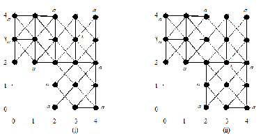
(i) If an endpoint of the horizontal through is in a vertical segment of and not in , replace the endpoint with one of the adjacent members of . E.g., with , replace with . This yields the -path .
(ii) If an endpoint of the horizontal through meets at the vertex of a right angle, replace the endpoint with the adjacent member of the incident vertical side of . E.g., with , replace with . This yields the -path .
8 More on the choice of adjacency
Example 8.1 below shows the importance of the adjacency used, since by Theorems 2.6 and 2.9, for the same sets and , with the adjacency, is a freezing set.
Example 8.1.
Let for . Let
Then, for , is an -cold set and not an -cold set.
Proof.
Let such that . By Proposition 3.1, the diagonals
| (5) |
Consider the digital triangle of points,
(see Figure 15).

Let . We will show that
| (6) |
Suppose otherwise. Then . Let . By the -continuity of , it follows from Lemma 3.2 that . Therefore, although . This is a contradiction, since . Thus (6) is established.
Next, we show
| (7) |
This follows from Lemma 3.2, since would imply , contrary to ; and would imply , contrary to .
Similarly, for a member of each of the following subsets of .
Since , we have for all . It follows that is an -cold set for .
To see is not an -cold set for , let be defined for by
(see Figure 16). Roughly, projects vertically to and leaves all other points of fixed. It is easy to see that , , and
Thus is not an -cold set for . ∎

9 Remarks on [17]
Much of this section is quoted or paraphrased from a comment posted to the website researchgate.com on the paper [17], by Kang and Han. The paper has a result that is original, correct and correctly proven, and interesting; however, the paper is greatly flawed. Some papers cited in [17] should not be rewarded with automated incremented citation counts, so papers cited in this section but not otherwise cited in the current paper are listed at the end of this section rather than among the references at the end of this paper. Papers cited elsewhere in the current paper are referenced as elsewhere in the current paper.
The paper [17] misguides readers through much of the literature of the almost fixed point property, also known as the approximate fixed point property (AFPP), for digital images. The AFPP generalizes the familiar fixed point property (FPP).
On page 7216, we find “ any digital space on does not have the FPP for (digitally) -continuous maps [21] (for more details, see [H19, H20]).” This statement is obviously false if has a single point; it is true when has more than one point (indeed, this case is noted on page 7218), the proof appearing in [11], a paper not cited in [17]. While [21] gives examples of digital images that lack the FPP, it says nothing like the general statement above attributed to it by [17]. Further, Han’s papers [H19, H20] contribute nothing to our knowledge of this assertion. Variants on these errors appear in the last paragraph of page 7218 of [17], where we also find Han’s paper [H17] falsely credited as a source for the FPP assertion above.
Also on page 7216, we find “ Banach contraction principle and a Cauchy sequence for complete metric spaces, we have also studied this issue” followed by citation of several papers. However, Cauchy sequences for digital metric spaces were shown in Han’s own paper [H16] to be trivial, and the Banach contraction principle was shown in [BxSt] to be trivial for digital images when the most natural metrics, including all metrics, are used. Indeed, most of the “contributions” for digital metric spaces in papers cited by [17] were shown in [BxSt] to be either trivial or incorrect.
Example 3.2(2) of [17] has no originality in either of its parts. Part (1-1) is implied by Theorem 3.5 of [5]. Both parts, (1-1) and (1-2), are implied by Theorem 4.8 of [6].
The adjacency given at Definition 4.1 of [17], attributed to Han’s paper [16], is the normal product adjacency. It was in the literature for decades before [16] appeared; see, e.g., [Ber].
Example 4.1 of [17] should have been derived as an immediate consequence of Theorem 3.3 of [21] and Theorem 4.2 of [11].
The only significant original contribution of [17] is its Theorem 4.4. The assertion that the normal product of and has the AFPP if the factors have the AFPP, is correctly proven. However, the implication that the factors have the AFPP if the product with the normal product adjacency has the AFPP, follows immediately and more simply from the fact that retractions preserve the AFPP [11]. Also, it should be noted that Theorem 4.4 generalizes Theorem 4.5 of [6].
References
[Ber] C. Berge, Graphs and Hypergraphs, 2nd edition. North-Holland,
Amsterdam, 1976.
[BxSt] L. Boxer and P.C. Staecker, Remarks on Fixed Point Assertions
in Digital Topology, Applied General Topology 20 (1) (2019), 135-153.
[H16] S.-E. Han, Banach fixed point theorem from the viewpoint of
digital topology,
Journal of Nonlinear Science and Applications
9 (2016), 895 - 905
[H17] S.-E. Han, Fixed point property for digital spaces,
Journal of Nonlinear Sciences and Applications, 10 (2017), 2510-2523
[H19] S.-E. Han, Remarks on the preservation of the almost
fixed point property involving several types
of digitizations, Mathematics, 7 (2019), 954.
[H20] S.-E. Han, Digital -contractibility of an -times
iterated connected sum of simple closed k-surfaces
and almost fixed point property, Mathematics, 8 (2020), 345
10 Further remarks
We have studied properties of cold sets for digital images in the digital plane. In sections 4 and 5, we have considered essential members of cold sets for . In sections 6 and 7, for the and adjacencies, respectively, we have derived cold sets for thick digital disks , with particular attention to convex disks. In section 8, we showed that the same sets , , can have very different cold-set properties depending on whether the adjacency considered is or .
The suggestions of an anonymous reviewer are acknowledged with gratitude.
References
- [1] L. Boxer, Digitally continuous functions, Pattern Recognition Letters 15 (1994), 833-839.
- [2] L. Boxer, A classical construction for the digital fundamental group, Journal of Mathematical Imaging and Vision 10 (1999), 51-62.
- [3] L. Boxer, Generalized normal product adjacency in digital topology, Applied General Topology 18 (2) (2017), 401-427
- [4] L. Boxer, Alternate product adjacencies in digital topology, Applied General Topology 19 (1) (2018), 21-53
- [5] L. Boxer, Approximate fixed point properties in digital topology, Bulletin of the International Mathematical Virtual Institute 10 (2) (2020), 357-367
- [6] L. Boxer, Approximate fixed point property for digital trees and products, Bulletin of the International Mathematical Virtual Institute 10(3) (2020), 595-602
- [7] L. Boxer, Fixed point sets in digital topology, 2, Applied General Topology 21(1) (2020), 111-133.
- [8] L. Boxer, Convexity and freezing sets in digital topology, Applied General Topology 22 (1) (2021), 121 - 137.
- [9] L. Boxer, Subsets and freezing sets in the digital plane, Hacettepe Journal of Mathematics and Statistics 50 (4) (2021), 991 - 1001
- [10]
L. Boxer,
Some consequences of restrictions on digitally
continuous functions, submitted. Available at
https://arxiv.org/submit/4163172 - [11] L. Boxer, O. Ege, I. Karaca, J. Lopez, and J. Louwsma, Digital fixed points, approximate fixed points, and universal functions, Applied General Topology 17(2), 2016, 159-172.
- [12] L. Boxer and P.C. Staecker, Fixed point sets in digital topology, 1, Applied General Topology 21 (1) (2020), 87-110.
- [13] L. Chen, Gradually varied surface and its optimal uniform approximation, SPIE Proceedings 2182 (1994), 300-307.
- [14] L. Chen, Discrete Surfaces and Manifolds, Scientific Practical Computing, Rockville, MD, 2004.
- [15] J. Haarmann, M.P. Murphy, C.S. Peters, and P.C. Staecker, Homotopy equivalence in finite digital images, Journal of Mathematical Imaging and Vision 53 (2015), 288-302.
- [16] S-E Han, Non-product property of the digital fundamental group, Information Sciences 171 (2005), 7391.
- [17] J.M. Kang and S-E. Han, The product property of the almost fixed point property for digital spaces AIMS Mathematics 6 (7) (2021), 7215-7228
- [18] T.Y. Kong and R. Kopperman, Digital topology, in K.P. Hart, Jun-iti Nagata, J.E. Vaughan, eds., Encyclopedia of General Topology, Elsevier, 2004
- [19] T.Y. Kong, R. Kopperman, and P.R. Meyer, A topological approach to digital topology, The American Mathematical Monthly 98 (10) (1991), 901-917
- [20] A. Rosenfeld, Digital topology, The American Mathematical Monthly 86 (8) (1979), 621-630.
- [21] A. Rosenfeld, ‘Continuous’ functions on digital pictures, Pattern Recognition Letters 4, 177-184, 1986.
- [22] R. Tsaur and M.B. Smyth, ‘Continuous’ multifunctions in discrete spaces with applications to fixed point theory, In: G. Bertrand, A. Imiya, R. Klette (eds.), Digital and Image Geometry, Lecture Notes in Computer Science, vol. 2243, 151-162. Springer, Berlin (2001), doi:10.1007/3-540-45576-05