跳到论文正文
W Papers独立论文阅读器 arXiv:2106.05980 论文正文 计算阅读时间 · 0%
引用这篇论文根据当前论文元数据生成,正式投稿前建议核对。


License: arXiv.org perpetual non-exclusive license
arXiv:2106.05980v1 [cond-mat.supr-con] 10 Jun 2021

Resistance of 2D superconducting films

E. J. König Affiliation: Max Planck Institute for Solid State Research, D-70569 Stuttgart, Germany    I. V. Protopopov Affiliation: Department of Theoretical Physics, University of Geneva, 1211 Geneva, Switzerland Affiliation: L. D. Landau Institute for Theoretical Physics RAS, 119334 Moscow, Russia    A. Levchenko Affiliation: Department of Physics, University of Wisconsin-Madison, Madison, Wisconsin 53706, USA    I. V. Gornyi Affiliation: Institute for Quantum Materials and Technologies, Karlsruhe Institute of Technology, 76021 Karlsruhe, Germany Affiliation: Institut für Theorie der kondensierten Materie, Karlsruhe Institute of Technology, 76128 Karlsruhe, Germany Affiliation: Ioffe Institute, 194021 St. Petersburg, Russia    A. D. Mirlin Affiliation: Institute for Quantum Materials and Technologies, Karlsruhe Institute of Technology, 76021 Karlsruhe, Germany Affiliation: Institut für Theorie der kondensierten Materie, Karlsruhe Institute of Technology, 76128 Karlsruhe, Germany Affiliation: L. D. Landau Institute for Theoretical Physics RAS, 119334 Moscow, Russia Affiliation: Petersburg Nuclear Physics Institute, 188300 St. Petersburg, Russia.
Abstract

We consider the problem of finite resistance RR in superconducting films with geometry of a strip of width WW near zero temperature. The resistance is generated by vortex configurations of the phase field. In the first type of process, quantum phase slip, the vortex worldline in 2+1 dimensional space-time is space-like (i.e., the superconducting phase winds in time and space). In the second type, vortex tunneling, the worldline is time-like (i.e., the phase winds in the two spatial directions) and connects opposite edges of the film. For moderately disordered samples, processes of second type favor a train of vortices, each of which tunnels only across a fraction of the sample. Optimization with respect to the number of vortices yields a tunneling distance of the order of the coherence length ξ\xi, and the train of vortices becomes equivalent to a quantum phase slip. Based on this theory, we find the resistance lnR∼−gW/ξ\ln R\sim-gW/\xi, where gg is the dimensionless normal-state conductance. Incorporation of quantum fluctuations indicates a quantum phase transition to an insulating state for g≲1g\lesssim 1.

Introduction. Since its original discovery by H. Kamerlingh Onnes a defining feature of superconductivity is its vanishing electrical resistivity in the thermodynamic limit. Yet, experimental samples are finite and can therefore be expected to display a non-zero, albeit small, resistance RR. This naturally provokes questions about the resistance of superconductors Huse et al. 1992; Halperin et al. 2011 – particularly in two-dimensional (2D) films, where resistivity and resistance have the same physical dimension: What is the dependence of RR on the system size and disorder strength? Is its scaling with increasing system size “dual” to the exponentially vanishing zero-temperature conductance of an insulator?

Refer to caption
Figure 1: (a) Setup for a prototypical measurement of resistance in a finite 2D superconducting film. (b) The bias current II lifts the periodicity of the ground state energy as a function of a fixed Δϕ=ϕ(L/2)−ϕ(−L/2)\Delta\phi=\phi(L/2)-\phi(-L/2). Tunneling events (and subsequent energy relaxation) between adjacent minima generate resistance. (c) Resistance, Eq. (9), per square (i.e., R​W/LRW/L) for several values of the normal-state conductance gg. The linearly decaying asymptotes of ln⁡R\ln R are consistent with experiment. Schneider et al. 2019

An approximate duality of this kind can be formalized Fisher 1990 using the particle-vortex duality within the bosonic description of the superconductor-insulator transition (SIT), Gantmakher and Dolgopolov 2010; Lin et al. 2015; Sacépé et al. 2020 when the normal state resistance is tuned to the quantum of resistance RQ≡h/4​e2R_{Q}\equiv h/4e^{2}. Such theories are optimized for samples, where Cooper pairs on superconducting granules Anderson-delocalize at the SIT. In this paper, instead, we concentrate on the different experimental situation of homogeneous films for which the impurity induced reduction and ultimate annulment of TcT_{c} (as defined by the onset of a spectral gap) is well described by fermionic theories Finkelstein 1990; Burmistrov et al. 2015 and the study of resistivity below TcT_{c} constitutes a separate, subsequent question: At finite temperature, but infinite system size, resistance is established by vortex proliferation above a renormalized Berezinskii-Kosterlitz-Thouless temperature. Halperin and Nelson 1979; König et al. 2015 On the other hand, near zero temperature, but at finite system size, the resistance as a function of size and disorder strength is unknown and is the subject of this paper. We focus on a 2D superconducting strip of width WW and length L>WL>W, Fig. 1a.

We begin by briefly reviewing the literature on the resistance of superconductors. Josephson’s equation relates the voltage V=(d​Δ​ϕ/d​t)​ℏ/2​eV=({d\Delta\phi}/{dt}){\hbar}/2e to the time derivative of the phase difference Δϕ=ϕ(x=L/2)−ϕ(x=−L/2){\Delta\phi=\phi(x=L/2)-\phi(x=-L/2)}. The presence of a bias current II lifts the degeneracy of quantum states with integer difference in Δ​ϕ/2​π\Delta\phi/2\pi, see Fig. 1b. Near zero temperature, quantum tunneling between adjacent minima dominates the decay of the phase difference. The voltage is then given by the effective tunneling rates 1/τ±2​π1/\tau_{\pm 2\pi} for the change of the phase by ±2​π\pm 2\pi,

V=h2​e​(1τ2​π−1τ−2​π).V=\frac{h}{2e}\left(\frac{1}{\tau_{2\pi}}-\frac{1}{\tau_{-2\pi}}\right). (1)

Theoretically, the decay of metastable vacua is described by instanton-like field configurations Vainshtein 1964; Langer 1967; Coleman 1977; Callan and Coleman 1977 i.e., imaginary-time solutions of the semiclassical equations of motion which connect the adjacent minima. For the decay of the supercurrent, the general form of such solutions is not known. However, certain trial solutions given by vortex configurations are believed to be good approximations. For the present strip geometry, those are the following: (i) vortex configurations which are yy-independent and swirl in the x−τx-\tau plane (τ\tau is the imaginary time), i.e., the worldline of the core is space-like; (ii) vortices which wind in the x−yx-y plane and tunnel across the system perpendicularly to the current (a time-like worldline). We will refer to case (i) as quantum phase slips and (ii) as vortex tunneling.

Most of the literature on the resistance of superconductors is devoted to thermally activated decay of the supercurrent Langer and Ambegaokar 1967; McCumber and Halperin 1970; Ovchinnikov and Varlamov 2015 and to vortex physics in the presence of a magnetic field Anderson 1962; Blatter et al. 1991; Blatter et al. 1994 or for current bias close to the critical current. We restrict ourselves to summarizing the work in the quantum regime for quasi-1D and 2D systems at small current and without external field. Supercurrent decay in homogeneous 1D wires was considered theoretically in Refs. [Saito and Murayama 1989; Duan 1995; Renn and Duan 1996; Zaikin et al. 1997a; Golubev and Zaikin 2001; Khlebnikov 2004; Refael et al. 2007]. There is a consensus that the semiclassically dominant field configuration is a dipole of phase slips at distance δ​τ∝1/I\delta\tau\propto 1/I in time direction, while the role of electromagnetic fields led to a debate Duan 1997; Zaikin et al. 1997b between the authors of Refs. [Duan 1995] and [Zaikin et al. 1997a]. In addition, it was shown that inhomogeneities in the wire can be crucially important. Pai et al. 2008; Vanević and Nazarov 2012 For 2D samples, studies of voltage generation in ultraclean samples focus on the theory of vortex tunneling,Ao and Thouless 1994; Iengo and Jug 1995; Iengo and Jug 1996; Arovas and Auerbach 2008 partly in terms of a very elegant mapping Popov 1973; Lee and Fisher 1991 to 2+1 dimensional electrodynamics. At the same time, the role of (i) finite width (ii) electromagnetic gauge potentials were disregarded in these works. Further, the influence of the Magnus force and the size of the vortex mass remained controversial (for review, see Ref. [Thouless et al. 1999]). Quantum tunneling in the presence of inhomogeneities (pinning centers) was addressed in Refs. [Feigel’man et al. 1993; Ao and Thouless 1994; Stephen 1994; Auerbach et al. 2006].

Experimental evidence Tafuri et al. 2006 for quantum tunneling of vortices in 2D superconductors at finite current bias, in particular in the context of dark photon counts,Kitaygorsky et al. 2007; Bulaevskii et al. 2011 additionally augmented the interest in this research field. New experimental tools, such as SQUID-on-tip microscopy,Embon et al. 2017 allow accessing both vortex motion and energy dissipation (local heating). At the same time, the direct measurement of the extremely small resistance of large samples of 2D superconductors is experimentally challenging; most recent studies Tamir et al. 2019 demonstrate the technical subtleties and advances in the careful filtering of external radiation. A remedy is to study higher-resistance samples, e.g., not too far from the SIT or with a smaller width WW. In the regime where a finite zero-temperature saturation value of RR is measurable, experimental data Schneider et al. 2019 is consistent with −ln⁡R∝W-\ln R\propto W.

In this work, we consider moderately disordered homogeneous films with 1/τel≫Δ2/EF1/\tau_{\rm el}\gg\Delta^{2}/E_{F} under infinitesimal current bias. We will refer to the case 1/τel≪Δ1/\tau_{\rm el}\ll\Delta (1/τel≫Δ1/\tau_{\rm el}\gg\Delta) as clean (dirty) limit. Here, EFE_{F} is the Fermi energy, τel\tau_{\rm el} the elastic scattering time of electrons, and Δ\Delta the spectral gap of the superconductor. As discussed below, for systems considered here the Magnus force is unimportant and the vortex mass is finite. We find that the combined tunneling of several vortices dominates over single-vortex events and demonstrate that, for the optimal number of involved vortices, the tunneling process has the same contribution as quantum phase slips. This allows us to determine the linear-response resistance of superconducting strips, which is exponentially small but finite. Estimating the preexponential factor and pushing the theory to the border of its applicability range, we also show that the SIT due to the antagonistic interplay of energy versus entropy (here due to quantum fluctuations) is captured at sufficiently strong disorder 1/τel∼EF1/\tau_{\rm el}\sim E_{F}.

Quantum phase slips. We first consider the voltage generation by quantum phase slips. In perfectly coherent systems, the decay out of a “false” vacuum is technically encoded in “bounce solutions”: Coleman 1977; Zaikin et al. 1997a a phase slip takes the system to a lower vacuum where it dwells for a time δ​τ\delta\tau and subsequently an anti-phase-slip takes it back to the point of departure. The action of a bounce is (Φ0\Phi_{0} is the flux quantum)

SI​(δ​τ)≃2​Score+K1​D​ln⁡(Δ​δ​τ)−Φ0​I​δ​τ.S_{I}(\delta\tau)\simeq 2S_{\rm core}+K_{\rm 1D}\ln(\Delta\delta\tau)-\Phi_{0}I\delta\tau. (2)

Each phase slip described by Eq. (2) is weighted by its core action Score∼K1​D∼(W/ξ)​EF​min⁡(τel,1/Δ)S_{\rm core}\sim K_{\rm 1D}\sim(W/\xi)E_{F}\min(\tau_{\rm el},1/\Delta), where the factor (W/ξ)(W/\xi) represents the length of the space-like worldline of the core. Here, we introduced the dimensionless stiffness of 1+1 dimensional (i.e., yy-independent) phase fluctuations K1​DK_{\rm 1D} and the coherence length ξ∼vF/Δ\xi\sim v_{F}/\Delta (ξ∼vF​τel/Δ\xi\sim v_{F}\sqrt{\tau_{\rm el}/\Delta}) in the clean (dirty) limit, where vFv_{F} is the Fermi velocity.

The action is maximal at the typical dwell time δ​τtyp=K1​D/(Φ0​I)\delta\tau_{\rm typ}=K_{\rm 1D}/(\Phi_{0}I), and a steepest-descent evaluation 1 of the instanton contribution to the partition sum Kleinert 2009 𝒵instanton∼(L/ξ)​∫d​δ​τ​exp⁡[−SI​(δ​τ)]\mathcal{Z}_{\rm instanton}\sim(L/\xi)\int d\delta\tau\exp[-S_{I}(\delta\tau)] yields the decay rate Zaikin et al. 1997a 1/τ2​π∼Δ2​δ​τtyp​exp⁡[−SI​(δ​τtyp)]​L/[ξ​K1​D]∼IK1​D−11/\tau_{2\pi}\sim\Delta^{2}\delta\tau_{\rm typ}\exp[{-S_{I}(\delta\tau_{\rm typ})}]L/[\xi\sqrt{K_{\rm 1D}}]\sim I^{K_{\rm 1D}-1}. This non-linear current-voltage characteristics is a manifestation of a perfectly quantum-coherent bounce. However, at infinitesimal bias current, δ​τtyp\delta\tau_{\rm typ} exceeds the relaxation time τcoh\tau_{\rm coh} which is always finite in a finite system connected to the metallic leads or in the presence of an external bath. The broadening of levels inside the core described by τcoh\tau_{\rm coh} leads to a finite rate for quantum phase slips and anti-phase-slips 1/τ±2​π∝e−S±I​(τcoh)​L/(τcoh​ξ).{1}/{\tau_{\pm 2\pi}}\propto e^{-S_{\pm I}(\tau_{\rm coh})}L/(\tau_{\rm coh}\xi). Then, Eq. (1) leads to a linear current-voltage relation,

RQPS∼he2LξK1​D−3/2(τcohΔ)2−K1​De−2​K1​D,R_{\rm{QPS}}\sim\frac{h}{e^{2}}\frac{L}{\xi}K_{\rm 1D}^{-3/2}\left(\tau_{\rm coh}\Delta\right)^{2-K_{\rm 1D}}e^{-2K_{\rm 1D}}, (3)

where the prefactor is determined by matching the non-linear resistance at I≳K1​D/(Φ0​τcoh)I\gtrsim K_{\rm 1D}/(\Phi_{0}\tau_{\rm coh}) mentioned above.

We conclude this consideration with three remarks. First, we comment on τcoh\tau_{\rm coh} which is finite in any realistic situation and may result from a variety of system-dependent origins, such as phonons, external radiation, and noise in the leads. Different sources generally imply different temperature and system-size dependence of the relaxation time which we do not study here, since the main factor in −ln⁡R-\ln R is the tunneling action, while τcoh\tau_{\rm coh} enters in the form of a logarithmic prefactor. Second, spatial fluctuation of the worldline of the phase-slip core around the y−y-independent line have been disregarded up to now. These fluctuations lead to an additional preexponential factor, which we estimate at the end of the paper. Third, magnetic screening effects (see Ref. [Duan 1997] and Supplement Sup) are unimportant in the above consideration Zaikin et al. 1997b so long as τcoh​Δ≪exp⁡(λM/W)\tau_{\rm coh}\Delta\ll\exp(\lambda_{M}/W), where λM\lambda_{M} is the Pearl length (2D analog of the London penetration length), which is usually macroscopic. For longer relaxation times, the result for −ln⁡R-\ln R gets modified according to K1​D​ln⁡(τcoh​Δ)→K1​D​λM​ln⁡[W​ln⁡(τcoh​Δ)/λM]/WK_{\rm 1D}\ln(\tau_{\rm coh}\Delta)\rightarrow K_{\rm 1D}\lambda_{M}\ln[W\ln(\tau_{\rm coh}\Delta)/\lambda_{M}]/W.

Vortex dynamics. When the width of the sample exceeds the superconducting coherence length, vortices in the x−yx-y plane of the superconducting film become well-defined topological excitations, and the supercurrent acquires an additional decay channel related to vortex tunneling across the sample. This effect therefore relies on the dynamics of vortices, described by the action:

Skin=∫d​τ​(m​x˙22+i​α​x˙​y)+η​∫d​ω2​π​|ω|​|x​(ω)|2,S_{\rm kin}=\int d\tau\left(\frac{m\dot{\textbf{{x}}}^{2}}{2}+i\,\alpha\,\dot{x}\,y\right)+\eta\int\frac{d\omega}{2\pi}|\omega||\textbf{{x}}(\omega)|^{2}, (4)

where x​(τ)=(x⁡(τ),y⁡(τ))\textbf{{x}}(\tau)=(x(\tau),y(\tau)) is the time-dependent position of a given vortex. The first term represents the kinetic energy for a point particle of mass mm, the term proportional to α\alpha describes the Magnus force, which is somewhat similar to the Lorentz force in a magnetic field, and the last term, proportional to η\eta, describes dissipation.

The values of these parameters drastically depend on whether the vortex core is featureless, or whether it contains a quasi-continuum of bound states. In the first case, dissipation is absent (η=0\eta=0) and the parameter α\alpha is topologically quantized (it is given by the superfluid density).Ao and Thouless 1993 The mass diverges logarithmically if the superfluid is neutral, but the logarithm is cut inside the core for charged superconductors, where the mass is therefore minute, m∼melectron​λTF/ξm\sim m_{\rm electron}\lambda_{\rm TF}/\xi (here, λTF\lambda_{\rm TF} is the Thomas-Fermi screening length).Suhl 1965; Brandt 1977; Duan and Leggett 1992; Duan 1993; Demircan et al. 1996

Here, we concentrate on the more realistic second case, in which the Caroli-deGennes-Matricon-type Caroli et al. 1964 bound states inside the vortex core cannot be neglected. In ss-wave superconductors, the spacing ω0\omega_{0} of these subgap states 2 can be estimated to be ω0∼ν−1​ξ−2\omega_{0}\sim\nu^{-1}\xi^{-2}, where ν\nu is the metallic density of states. Typically, in the clean (dirty) limit, ω0∼Δ2/EF\omega_{0}\sim\Delta^{2}/E_{F} (ω0∼Δ/EF​τel\omega_{0}\sim\Delta/E_{F}\tau_{\rm el}) is negligible compared to 1/τel1/\tau_{\rm el}. For a moving vortex that explores different microscopic realizations of disorder, this leads to a quasi-continuum of states, which allows for energy dissipation, yielding η∼n​ω0​τel\eta\sim n\omega_{0}\tau_{\rm el}, where nn is the density of electrons in the normal state. Bardeen and Stephen 1965; Feigel’man et al. 1993 At the same time, the Magnus force acquires a second topological contribution resulting from the spectral flow of bound states, which is equal in magnitude but opposite to the hydrodynamic contribution discussed above, so that α\alpha effectively vanishes. Kopnin and Kravtsov 1976; Volovik 2003 Finally, the vortex mass is given by the total mass of particles trapped inside the vortex, m∼melectron​ξ2/λF2m\sim m_{\rm electron}\xi^{2}/\lambda_{F}^{2}. Volovik 2003

Refer to caption
Figure 2: Cartoon of a single vortex at position (x0,y0)(x_{0},y_{0}) tunneling from lower to the upper edge. (a),(c),(e): Gradient of the superconducting phase ∇ϕ\nabla\phi. Note that mirror charges outside the sample (gray shaded) ensure no current outflux. (b),(d),(f): Vector field (cos⁡(ϕ),sin⁡(ϕ))(\cos(\phi),\sin(\phi)). Our choice for the branch cut is represented by a pink zig-zag line. (g), (h), (i): Principal branch of the phase ϕ\phi along the colored horizontal lines of panels (a)-(f) (same color and dashing code).

Single vortex tunneling. Let us now inspect tunneling events involving a single vortex in the system. We remind the reader of the logarithmic attraction of a vortex-antivortex pair, which physically reflects the principle of minimizing the region of costly superflow between defects of opposite winding. It is, perhaps, less known that a single vortex in a finite superconducting strip is attracted to the boundaries. Technically, this results from the implementation of no-current-outflux boundary conditions by means of mirror charges (see Fig. 2a,c,e and Supplement Sup) and leads to a potential V⁡(y)=2​J​ln⁡[W​cos⁡(π​y/W)/ξ]V(y)=2J\ln[W{\cos(\pi y/W)}/{\xi}], that should be included in the total action of the vortex in the strip geometry. Here, JJ is the 2D superconducting stiffness: J∼EFJ\sim E_{F} (J∼EF​Δ​τelJ\sim E_{F}\Delta\tau_{\rm el}) in the clean (dirty) limit at zero temperature.

We begin by considering a ‘kink solution’, ykink​(τ)y_{\rm kink}(\tau), of the equation of motion, i.e., the unbinding of a single vortex from lower boundary and subsequent tunneling across the system, see Fig. 2 for illustration. The tunneling action is Skink​(W)=Spot​(W)+Scond​(W)S_{\rm kink}(W)=S_{\rm pot}(W)+S_{\rm cond}(W), where

Spot\displaystyle S_{\rm pot} =∫−W/2+ξW/2−ξdy2​m​V​(y)=2Wm​Jf(πξ/W),\displaystyle=\int_{-W/2+\xi}^{W/2-\xi}\!dy\sqrt{2mV(y)}=2W\sqrt{mJ}f(\pi\xi/W), (5)

is the contribution from the potential barrier. Here, we have introduced the dimensionless function f⁡(x)f(x) that satisfies f⁡(x)≃ln⁡(1/x)f(x)\simeq\sqrt{\ln(1/x)} in the limit x≪1x\ll 1 and f⁡(π/2)=0f(\pi/2)=0. The second contribution, Scond=Econd​𝒯S_{\rm cond}=E_{\rm cond}\mathcal{T}, is the condensation energy Econd∼JE_{\rm cond}\sim J times the total length of the worldline 𝒯=𝒯⁡(W)\mathcal{T}=\mathcal{T}(W). Here, 𝒯⁡(W)=W/[v​ln⁡(W/π​ξ)]\mathcal{T}(W)=W/[v\sqrt{\ln(W/\pi\xi)}] for wide strips W≫ξW\gg\xi (with v=J/m∼vF​Δ/EFv=\sqrt{J/m}\sim v_{F}\Delta/E_{F} the typical vortex speed), whereas for W→2​ξW\rightarrow 2\xi, 𝒯⁡(W)→1/Δ\mathcal{T}(W)\rightarrow 1/\Delta, which is the time for a vortex to nucleate. Thus, for narrow strips, Skink​(W→2​ξ)≃J/Δ∼K1​D|W∼ξ{S_{\rm kink}(W\rightarrow 2\xi)\simeq~J/\Delta}\sim K_{\rm 1D}|_{W\sim\xi} approaches the same value as the core action of a quantum phase slip, while for wide strips, both Spot​(W)S_{\rm pot}(W) and Scond​(W)S_{\rm cond}(W) are of the order of J​W/v∼(W/λF)​EF​min⁡(τel,1/Δ)JW/v\sim(W/\lambda_{F})E_{F}\min(\tau_{\rm el},1/\Delta), which is (ξ/λF)(\xi/\lambda_{F}) times larger than the core action of a phase slip in Eq. (2).

A finite current bias lifts the degeneracy of the potential minima at y=±W/2y=\pm W/2 by an additional term VI=−Φ0Iy/WV_{I}=-\Phi_{0}Iy/W. As mentioned, the supercurrent decay is governed by a bounce solution, Coleman 1977; Kleinert 2009 which we approximate by a kink and an antikink at temporal distance δ​τ\delta\tau: ybounce​(τ)=ykink​(τ+δ​τ/2)−ykink​(τ−δ​τ/2)+W/2−ξy_{\rm bounce}(\tau)=y_{\rm kink}(\tau+\delta\tau/2)-y_{\rm kink}(\tau-\delta\tau/2)+W/2-\xi. Using this Ansatz, we obtain the following δ​τ\delta\tau-dependent action, see Supplement Sup,

SI​(δ​τ)\displaystyle S_{I}(\delta\tau) =2​Skink​(W)+Sint​(δ​τ)−Φ0​I​δ​τ.\displaystyle=2S_{\rm kink}(W)+S_{\rm int}(\delta\tau)-\Phi_{0}I\delta\tau. (6)

At variance with the 1D bounce solution, Eq. (2), the attraction between kink and antikink, encoded in Sint​(δ​τ)S_{\rm int}(\delta\tau), can not be determined exactly. It asymptotically vanishes if the vortex disappears at the opposite boundary,3 Sint​(δ​τ)→0S_{\rm int}(\delta\tau)\to 0 for δ​τ>𝒯\delta\tau>\mathcal{T} and monotonically increases in the preceding regime 0<𝒯−δ​τ≪𝒯0<\mathcal{T}-\delta\tau\ll\mathcal{T}, where Sint​(δ​τ)≃−Econd​(𝒯−δ​τ)S_{\rm int}(\delta\tau)\simeq-E_{\rm cond}(\mathcal{T}-\delta\tau), which shows that the dominant reason for attraction is the string tension of the vortex worldline.

Formally, the instanton contribution to the partition sum can be evaluated using the steepest-descent method analogously to the bounce action (2). However, the properties of Sint​(δ​τ)S_{\rm int}(\delta\tau) imply that the typical dwell time δ​τ\delta\tau diverges as a function of I→0I\rightarrow 0, exceeding the coherence time τcoh≫𝒯\tau_{\rm coh}\gg\mathcal{T}. Consequently, evaluation of Eq. (1) similarly to (3) but using Eq. (6) instead of Eq. (2) yields

RSVT=he2​Lξ​𝒜vortex​e−2​Skink​(W).R_{\rm{SVT}}=\frac{h}{e^{2}}\frac{L}{\xi}\mathcal{A}_{\rm vortex}\ e^{-2S_{\rm kink}(W)}. (7)

The pre-exponential factor 𝒜vortex\mathcal{A}_{\rm vortex} depends on the nature of relaxation and should be evaluated for a given microscopic model of relaxation.

We conclude the discussion of a single-vortex tunneling with three comments. First, the logarithmic vortex interaction is cut beyond the Pearl lengthSup λM\lambda_{M}so that Eq. (5) is valid only for samples W<λMW<\lambda_{M}. Second, the effect of dissipation on the tunneling has been disregarded here, which is valid if the tunneling time 𝒯\mathcal{T} is small compared to the dissipation time m/η∼1/ω02​τelm/\eta\sim 1/\omega_{0}^{2}\tau_{\rm el}. This is equivalent to the condition W≪min​(vF​τel,ξ)/(ω0​τel)W\ll\text{min}(v_{F}\tau_{\rm el},\xi)/(\omega_{0}\tau_{\rm el}). We will see in the next section that the resistance is dominated by vortices tunneling across an effective distance dopt≪Wd_{\rm opt}\ll W, which satisfies both the bounds imposed by screening and by dissipation, even for wide junctions. Third, in deriving the effective tunneling action, we disregarded the mesoscopic fluctuations of the superconducting gap (and, hence, stiffness JJ). Skvortsov and Feigel’man 2005; König et al. 2015 As we demonstrate in Ref. [Sup] for EF​τel≫1E_{F}\tau_{\rm el}\gg 1, these fluctuations do not affect the exponential factor in Eq. (7).

Refer to caption
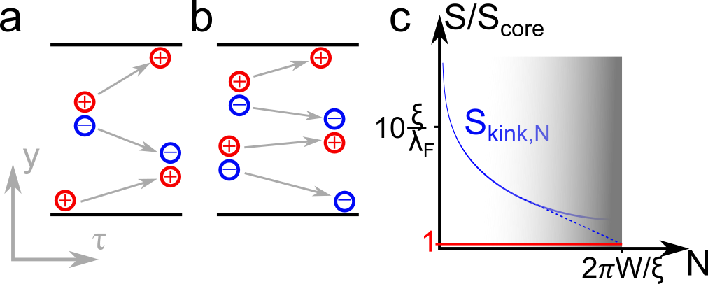
Figure 3: Multi-vortex tunneling processes. (a) The unbinding of a vortex from the lower edge, similar to Fig. 2, but assisted by an additional dipole nucleating in the bulk of the system. (b) The decay of two vortex dipoles into a dipole and two vortices disappearing at the edge. (c) The tunneling action (in units of ScoreS_{\rm core} introduced in Eq. (2)) for a multi-vortex tunneling process as a function of NN.

Multi-vortex tunneling. A simple tunneling event that involves more than one vortex is a dipole dissociation,Iengo and Jug 1995 in which a quantum fluctuation creates a dipole of vortices inside the strip and subsequently the dipole constituents tunnel towards opposite edges, leading to an overall phase slip of 2​π2\pi. Here, we consider a generalization of this event where nn dipoles are nucleated in the strip and subsequently tunnel to either side of the strip, see Fig. 3b. We also consider a generalization of the edge unbinding event discussed above, Fig. 2, where the tunneling of a vortex from one edge to the other is assisted by nn dipoles in the bulk, see Fig. 3a.

As a natural Ansatz, we consider (see SupplementSup) the total action Skink,N=∑i=1NSkink​(di)S_{\rm kink,N}=\sum_{i=1}^{N}S_{\rm kink}(d_{i}), where Skink​(d)S_{\rm kink}(d) is the kink action for a single vortex tunneling in a strip of size dd introduced before Eq. (5), did_{i} is the tunneling distance of the iith vortex, and N=2​n+1N=2n+1 in the case of Fig. 3a and N=2​nN=2n in case of Fig. 3b. The minimization of the action prescribes that all dipoles nucleate at the same moment in time and same xx-position, and that the nucleation points are furthermore equally spaced in yy-direction, i.e., each vortex travels the same distance dN=W/Nd_{N}=W/N, so that the kink action is Skink,N=N​Skink​(dN)S_{\rm kink,N}=NS_{\rm kink}(d_{N}). We remark that this is an accurate tunneling action for the optimum event; yet, the Ansatz that we used is heuristic and employing it for the calculation of fluctuation determinant is not exact, although parametrically correct.

Increasing NN in Skink,NS_{\rm kink,N} has two effects. On one hand, N​Spot​(dN)NS_{\rm pot}(d_{N}) decreases with the number of dipoles. On the other hand, the contribution of the string tension N​Econd​𝒯​(dN)NE_{\rm cond}\mathcal{T}(d_{N}) increases with NN (even though 𝒯⁡(dN)\mathcal{T}(d_{N}), of course, decreases). The first effect prevails, see Fig. 3c, in which the solid curve is obtained on the basis of the vortex motion at length scales large compared to ξ\xi, and the dashed curve is the extrapolation of 𝒯⁡(dN)↘1/Δ\mathcal{T}(d_{N})\searrow 1/\Delta as dNd_{N} approaches ξ\xi (shaded region). The action is monotonically decreasing with increasing number of vortices, leading to an optimum number Nopt∼W/ξN_{\rm opt}\sim W/\xi and dN∼2​ξd_{N}\sim 2\xi. The resistance produced by multi-vortex configurations,

RMVT=he2​Lξ​𝒜​e−2​(W/ξ)​Skink​(2​ξ)R_{\rm MVT}=\frac{h}{e^{2}}\frac{L}{\xi}\mathcal{A}\ e^{-2(W/\xi)S_{\rm kink}(2\xi)} (8)

follows along the lines of the calculation for the single-vortex tunneling event (the preexponential factor 𝒜\mathcal{A}, which may depend on relaxation details, is considered separately). Clearly, as dN∼ξd_{N}\sim\xi, vortices cease being well-defined excitations, and the multi-vortex tunneling event cannot be distinguished from a quantum phase slip. It is, therefore, a reassuring consistency check that the exponent in the resistance due to NN co-tunneling vortices, Eq. (8), N​Skink​(2​ξ)∼N​J/Δ∼W​EF​min⁡(1/Δ,τel)/ξ∼K1​DNS_{\rm kink}(2\xi)\sim NJ/\Delta\sim WE_{F}\min(1/\Delta,\tau_{\rm el})/\xi\sim K_{\rm 1D}, is in accordance with the exponent of the resistance due to quantum phase slips, Eq. (3).

Conclusion. In summary, we have investigated the resistance of superconducting strips with moderate disorder 1/τel≫Δ2/EF1/\tau_{\rm el}\gg\Delta^{2}/E_{F} near zero temperature. The obtained resistance RR is dominated by cotunneling of N∼W/ξ>1N\sim W/\xi>1 vortices, a process that is equivalent to a quasi-1D quantum phase slip. This yields ln⁡R∼−(W/ξ)​EF​min⁡(1/Δ,τel)\ln R\sim-(W/\xi)E_{F}\min(1/\Delta,\tau_{\rm el}), see Eqs. (3) and (8), which qualitatively agrees with the low-TT saturation values of resistance presented in Fig. 1 of Ref. [Schneider et al. 2019]. Our result for exponential dependence of resistance on WW is reminiscent of exponential suppression of conductance with the system size on the insulating side of SIT.

While we concentrated on the exponent of the superconducting decay rate, we conclude with a discussion of the preexponential factor. Its WW-dependence stems from quantum fluctuations of the tunneling trajectory, only, if the mechanism of dissipation is local. Using the above-mentioned Ansatz for multi-vortex events, we estimate that each of the W/ξW/\xi vortices contributes to 𝒜\mathcal{A} in Eq. (8) a fluctuation determinant of the order of the inverse kink action,Sup leading to a preexponential factor [Skink(2ξ)]−W/ξ[S_{\rm kink}(2\xi)]^{-W/\xi}. (A similar factor is expected to arise from spatial fluctuations about the straight yy-independent phase-slip world-line.) By re-exponentiation, this quantum-fluctuation-induced prefactor can be viewed as an entropic contribution to the tunneling action, leading to

ln(e2R/h)∼−W[g+ln(g)]/ξ+ln(L/ξ),\ln(e^{2}R/h)\sim-W[g+\ln(g)]/\xi+\ln(L/\xi)\,, (9)

where, in the dirty limit, Skink​(2​ξ)∼EF​τel≡gS_{\rm kink}(2\xi)\sim E_{F}\tau_{\rm el}\equiv g is given by the normal-state conductance, see Fig. 1c. Pushing our theory to the limit of its applicability, we observe a sign change of the action at g∼1g\sim 1, reminiscent of SIT.

We acknowledge useful discussions with D. Bagrets, A.  Bezryadin, I. Burmistrov, A. Finkelstein, E. Khalaf, A. Rogachev, D. Shahar, M. Skvortsov, C. Strunk, H. Xie, and A. Zaikin. Support for this work at the University of Wisconsin-Madison (A.L.) was provided by the National Science Foundation, Quantum Leap Challenge Institute for Hybrid Quantum Architectures and Networks, NSF Grant No. 2016136.

References

  • Huse et al. (1992) D. A. Huse, M. P. Fisher, and D. S. Fisher, Nature 358, 553 (1992).
  • Halperin et al. (2011) B. I. Halperin, G. Refael, and E. Demler, in BCS: 50 Years, edited by L. Cooper and D. Feldman (World Scientific, 2011).
  • Schneider et al. (2019) I. Schneider, K. Kronfeldner, T. I. Baturina, and C. Strunk, Phys. Rev. B 99, 094522 (2019).
  • Fisher (1990) M. P. A. Fisher, Phys. Rev. Lett. 65, 923 (1990).
  • Gantmakher and Dolgopolov (2010) V. F. Gantmakher and V. T. Dolgopolov, Physics-Uspekhi 53, 1 (2010).
  • Lin et al. (2015) Y.-h. Lin, J. Nelson, and A. M. Goldman, Physica C: Superconductivity and its applications 514, 130 (2015).
  • Sacépé et al. (2020) B. Sacépé, M. Feigel’man, and T. M. Klapwijk, Nature Physics 16, 734 (2020).
  • Finkelstein (1990) A. Finkelstein, Sov. Sci. Rev., Sect. A 14, 1 (1990).
  • Burmistrov et al. (2015) I. S. Burmistrov, I. V. Gornyi, and A. D. Mirlin, Phys. Rev. B 92, 014506 (2015).
  • Halperin and Nelson (1979) B. Halperin and D. Nelson, Journal of Low Temperature Physics 36, 599 (1979).
  • König et al. (2015) E. J. König, A. Levchenko, I. V. Protopopov, I. V. Gornyi, I. S. Burmistrov, and A. D. Mirlin, Phys. Rev. B 92, 214503 (2015).
  • Vainshtein (1964) A. Vainshtein, “Decaying systems and divergence of the series of perturbation theory,” (1964), Novosibirsk Institute of Nuclear Physics Report (preprint).
  • Langer (1967) J. Langer, Annals of Physics 41, 108 (1967).
  • Coleman (1977) S. Coleman, Phys. Rev. D 15, 2929 (1977).
  • Callan and Coleman (1977) C. G. Callan and S. Coleman, Phys. Rev. D 16, 1762 (1977).
  • Langer and Ambegaokar (1967) J. Langer and V. Ambegaokar, Phys. Rev. 164, 498 (1967).
  • McCumber and Halperin (1970) D. E. McCumber and B. I. Halperin, Phys. Rev. B 1, 1054 (1970).
  • Ovchinnikov and Varlamov (2015) Y. N. Ovchinnikov and A. A. Varlamov, Phys. Rev. B 91, 014514 (2015).
  • Anderson (1962) P. W. Anderson, Phys. Rev. Lett. 9, 309 (1962).
  • Blatter et al. (1991) G. Blatter, V. B. Geshkenbein, and V. M. Vinokur, Phys. Rev. Lett. 66, 3297 (1991).
  • Blatter et al. (1994) G. Blatter, M. V. Feigel’man, V. B. Geshkenbein, A. I. Larkin, and V. M. Vinokur, Rev. Mod. Phys. 66, 1125 (1994).
  • Saito and Murayama (1989) S. Saito and Y. Murayama, Physics Letters A 139, 85 (1989).
  • Duan (1995) J.-M. Duan, Phys. Rev. Lett. 74, 5128 (1995).
  • Renn and Duan (1996) S. R. Renn and J.-M. Duan, Phys. Rev. Lett. 76, 3400 (1996).
  • Zaikin et al. (1997a) A. D. Zaikin, D. S. Golubev, A. van Otterlo, and G. T. Zimányi, Phys. Rev. Lett. 78, 1552 (1997a).
  • Golubev and Zaikin (2001) D. S. Golubev and A. D. Zaikin, Phys. Rev. B 64, 014504 (2001).
  • Khlebnikov (2004) S. Khlebnikov, Phys. Rev. Lett. 93, 090403 (2004).
  • Refael et al. (2007) G. Refael, E. Demler, Y. Oreg, and D. S. Fisher, Phys. Rev. B 75, 014522 (2007).
  • Duan (1997) J.-M. Duan, Phys. Rev. Lett. 79, 3316 (1997).
  • Zaikin et al. (1997b) A. D. Zaikin, D. S. Golubev, A. van Otterlo, and G. T. Zimányi, Phys. Rev. Lett. 79, 3317 (1997b).
  • Pai et al. (2008) G. V. Pai, E. Shimshoni, and N. Andrei, Phys. Rev. B 77, 104528 (2008).
  • Vanević and Nazarov (2012) M. Vanević and Y. V. Nazarov, Phys. Rev. Lett. 108, 187002 (2012).
  • Ao and Thouless (1994) P. Ao and D. J. Thouless, Phys. Rev. Lett. 72, 132 (1994).
  • Iengo and Jug (1995) R. Iengo and G. Jug, Phys. Rev. B 52, 7537 (1995).
  • Iengo and Jug (1996) R. Iengo and G. Jug, Phys. Rev. B 54, 13207 (1996).
  • Arovas and Auerbach (2008) D. P. Arovas and A. Auerbach, Phys. Rev. B 78, 094508 (2008).
  • Popov (1973) V. Popov, Sov. Phys. JETP 37, 341 (1973), [ZhETF 64, 672 (1973)].
  • Lee and Fisher (1991) D.-H. Lee and M. P. Fisher, International Journal of Modern Physics B 05, 2675 (1991).
  • Thouless et al. (1999) D. J. Thouless, P. Ao, Q. Niu, M. R. Geller, and C. Wexler, International Journal of Modern Physics B 13, 675 (1999).
  • Feigel’man et al. (1993) M. Feigel’man, V. Geshkenbein, A. Larkin, and S. Levit, JETP Lett. 57, 711 (1993).
  • Stephen (1994) M. J. Stephen, Phys. Rev. Lett. 72, 1534 (1994).
  • Auerbach et al. (2006) A. Auerbach, D. P. Arovas, and S. Ghosh, Phys. Rev. B 74, 064511 (2006).
  • Tafuri et al. (2006) F. Tafuri, J. R. Kirtley, D. Born, D. Stornaiuolo, P. G. Medaglia, P. Orgiani, G. Balestrino, and V. G. Kogan, Europhysics Letters 73, 948 (2006).
  • Kitaygorsky et al. (2007) J. Kitaygorsky et al., IEEE Trans. Appl. Supercond. 17, 275 (2007).
  • Bulaevskii et al. (2011) L. N. Bulaevskii, M. J. Graf, C. D. Batista, and V. G. Kogan, Phys. Rev. B 83, 144526 (2011).
  • Embon et al. (2017) L. Embon, Y. Anahory, Z. L. Jelić, E. O. Lachman, Y. Myasoedov, M. E. Huber, G. P. Mikitik, A. V. Silhanek, M. V. Milosević, A. Gurevich, et al., Nature Communications 8, 1 (2017).
  • Tamir et al. (2019) I. Tamir, A. Benyamini, E. Telford, F. Gorniaczyk, A. Doron, T. Levinson, D. Wang, F. Gay, B. Sacépé, J. Hone, et al., Science Advances 5, eaau3826 (2019).
  • (48) Reference Zaikin et al. 1997a evaluated the integral ∫d​δ​τ​exp⁡[−S⁡(δ​τ)]\int d\delta\tau\exp[-S(\delta\tau)] exactly and found an exponent R∼IK1​D−2R\sim I^{K_{\rm 1D}-2}. It is in agreement with the result R∼IK1​D−1R\sim I^{K_{\rm 1D}-1} of the steepest-descent method used in our work in its regime of applicability, K1​D≫1K_{\rm 1D}\gg 1. The advantage of our approach is that it is applicable for both quantum phase slips and 2D vortex tunneling.
  • Kleinert (2009) H. Kleinert, Path Integrals in Quantum Mechanics, Statistics, Polymer Physics, and Financial Markets, EBL-Schweitzer (World Scientific, 2009).
  • (50) Supplementary materials to this publication, which include Refs. [Abrahams and Tsuneto 1966; Stoof 1993].
  • Ao and Thouless (1993) P. Ao and D. J. Thouless, Phys. Rev. Lett. 70, 2158 (1993).
  • Suhl (1965) H. Suhl, Phys. Rev. Lett. 14, 226 (1965).
  • Brandt (1977) E. Brandt, Journal of Low Temperature Physics 26, 735 (1977).
  • Duan and Leggett (1992) J.-M. Duan and A. J. Leggett, Phys. Rev. Lett. 68, 1216 (1992).
  • Duan (1993) J.-M. Duan, Phys. Rev. B 48, 333 (1993).
  • Demircan et al. (1996) E. Demircan, P. Ao, and Q. Niu, Phys. Rev. B 54, 10027 (1996).
  • Caroli et al. (1964) C. Caroli, P. De Gennes, and J. Matricon, Physics Letters 9, 307 (1964).
  • (58) In what follows, a possible “zero-bias anomaly” structure in the density of the core bound states (peak or dip, depending on the strength of disorder Caroli et al. 1964; Datta et al. 2021) will be inessential for our analysis.
  • Bardeen and Stephen (1965) J. Bardeen and M. J. Stephen, Phys. Rev. 140, A1197 (1965).
  • Kopnin and Kravtsov (1976) N. Kopnin and V. Kravtsov, JETP Lett. 23, 578 (1976).
  • Volovik (2003) G. E. Volovik, The universe in a helium droplet, Vol. 117 (Oxford University Press on Demand, 2003).
  • (62) Here, we do not describe microscopically the process of vortex disappearance at the boundary, assuming that the relaxation described by τcoh\tau_{\text{coh}} is sufficient for transferring the core electrons to the condensate or to the leads.
  • Skvortsov and Feigel’man (2005) M. A. Skvortsov and M. V. Feigel’man, Phys. Rev. Lett. 95, 057002 (2005).
  • Abrahams and Tsuneto (1966) E. Abrahams and T. Tsuneto, Phys. Rev. 152, 416 (1966).
  • Stoof (1993) H. T. C. Stoof, Phys. Rev. B 47, 7979 (1993).
  • Datta et al. (2021) A. Datta, A. Banerjee, N. Trivedi, and A. Ghosal, “New paradigm for a disordered superconductor in a magnetic field,” (2021), arXiv:2101.00220 [cond-mat.supr-con] .

Supplementary materials on

”Resistance of 2D superconducting films”
Elio J. König1, I. V. Protopopov2,3, A. Levchenko4, I.V. Gornyi5,6,7, A. D. Mirlin5,6,3,8

1Max Planck Institute for Solid State Research, D-70569 Stuttgart, Germany

2Department of Theoretical Physics, University of Geneva, 1211 Geneva, Switzerland

3L. D. Landau Institute for Theoretical Physics RAS, 119334 Moscow, Russia

4Department of Physics, University of Wisconsin-Madison, Madison, Wisconsin 53706, USA

5Institute for Quantum Materials and Technologies, Karlsruhe Institute of Technology, 76021 Karlsruhe, Germany

6Institut für Theorie der kondensierten Materie, Karlsruhe Institute of Technology, 76128 Karlsruhe, Germany

7Ioffe Institute, 194021 St. Petersburg, Russia

8Petersburg Nuclear Physics Institute, 188300 St. Petersburg, Russia

These supplementary materials contain an overview of list of scales, Sec. S-I, employed in the paper, a derivation of the vortex interaction in the strip with and without screening (Secs. S-II, S-III, respectively), details about vortex tunneling, Sec. S-IV, about the multivortex tunneling configurations, Sec. S-V and about the effect of mesoscopic fluctuations, Sec. S-VI.

S-I List of scales

S-I.1 List of energy and time scales

  • •

    elastic scattering time τel\tau_{\rm el}.

  • •

    coherence time 1/Δ1/\Delta

  • •

    Tunneling time 𝒯\mathcal{T}

  • •

    2+1 D stiffness JJ at zero temperature. Clean case: J∼EFJ\sim E_{F}. Dirty case: J=Δ​EF​τelJ=\Delta E_{F}\tau_{\rm el}.

S-I.2 List of length scales

  • •

    Fermi wave length λF\lambda_{F}

  • •

    UV length scale λ0\lambda_{0}. Clean case: λ0=λF\lambda_{0}=\lambda_{F}. Dirty case: λ0=λF/Δ​τel\lambda_{0}=\lambda_{F}/\sqrt{\Delta\tau_{\rm el}}

  • •

    Thomas Fermi wave length λTF\lambda_{\rm TF}

  • •

    Coherence length ξ\xi. Clean case: ξ=vF/Δ\xi=v_{F}/\Delta, dirty case: ξ=vF​Δ/τel\xi=v_{F}\sqrt{\Delta/\tau_{\rm el}}.

  • •

    Pearl length λM=λTF​c2/v02\lambda_{M}=\lambda_{\rm TF}c^{2}/v_{0}^{2}.

S-II Vortex interaction parameters and screening

For the convenience of the reader, this section summarizes basic properties of vortex interactions in the finite strip.

S-II.1 Long-wavelength action

We consider the following effective long-wavelength action of the superconducting plate, see Fig. 1

S=∫(x,y,τ)[Jπ​(2​ec​A−∇ϕ)2+Zπ​(2​e​A0+∂τϕ)2],S=\int_{(x,y,\tau)}\left[\frac{J}{\pi}\left(\frac{2e}{c}\textbf{{A}}-\nabla\phi\right)^{2}+\frac{Z}{\pi}\left(2eA_{0}+\partial_{\tau}\phi\right)^{2}\right], (S1)

where ∫(x,y,τ)=∫−L/2L/2dx∫−W/2W/2dy∫−∞∞dτ\int_{(x,y,\tau)}=\int_{-L/2}^{L/2}dx\int_{-W/2}^{W/2}dy\int_{-\infty}^{\infty}d\tau, supplemented with the Maxwell action of electromagnetic fields (A0,A→)(A_{0},\vec{A}) living in (3+1) dimensional space-time. As the phase field ϕ\phi may contain singularities it is important to keep in mind that ∇→​ϕ\vec{\nabla}\phi is in general not a gradient field. The notation used in Eq. (S1) is suggestive and mathematically correct only away from the singularities.

The parameters J,ZJ,Z of this action define a characteristic length scale λ0=1/J​Z\lambda_{0}=1/\sqrt{JZ} and speed v0=J/Zv_{0}=\sqrt{J/Z}.Abrahams and Tsuneto 1966; Stoof 1993 In addition, they define length scales associated to the screening of electric charge λTF=1/[16​e2​Z]∼λ0​v0/[αQED​c]\lambda_{\rm TF}=1/[16{e^{2}}Z]\sim\lambda_{0}v_{0}/[\alpha_{\rm QED}c] (“Thomas-Fermi length”) and current λM=c2/[16​e2​J]=λTF​c2/v02∼λ0​c/[αQED​v0]\lambda_{M}=c^{2}/[16e^{2}J]=\lambda_{\rm TF}{c^{2}}/{v_{0}^{2}}\sim\lambda_{0}c/[\alpha_{\rm QED}v_{0}] (“Pearl-London length”), where 1/αQED≈1371/\alpha_{\rm QED}\approx 137 if the sample is suspended in vacuum.

In our calculations, we use v0≪cv_{0}\ll c and additionally assume the following realistic hierarchy of length scales L≫{W,λM}≫ξ≫{λTF,λ0}L\gg\{W,\lambda_{M}\}\gg\xi\gg\{\lambda_{\rm TF},\lambda_{0}\}. Note that, in typical experimental samples, the Pearl-London length, which is about four to five orders of magnitude larger than λ0≳1​n​m\lambda_{0}\gtrsim 1nm, can be smaller, larger or comparable to the system’s width.

Since we are considering a charged superconductor, the smooth part of the Goldstone mode ϕ\phi can be reabsorbed in a redefinition of the electromagnetic fields (A0,A)(A_{0},\textbf{{A}}) (“Anderson-Higgs-mechanism”). However, singular configurations of ϕ\phi, such as vortices, and an externally applied current bias can not be “eaten” by a gauge transformation of the vector potential. Differentiation of the action (S1) with respect to the gauge potentials (A0,A)(A_{0},\textbf{{A}}) implies the 2D charge and current densities, ρ\rho and jtot=j+j0​e^x\textbf{{j}}_{\rm tot}=\textbf{{j}}+j_{0}\hat{e}_{x}, respectively, where

ρ\displaystyle\rho =\displaystyle= −4​e​Zπ​(∂τψ+2​e​A0),\displaystyle-4e\frac{Z}{\pi}\left(\partial_{\tau}\psi+2eA_{0}\right), (S2a)
j =\displaystyle= 4​ec​Jπ​(∇ψ−2​ec​A),\displaystyle\frac{4e}{c}\frac{J}{\pi}\left(\nabla\psi-\frac{2e}{c}\textbf{{A}}\right), (S2b)
and
j0≡IW​c=c​o​n​s​t.j_{0}\equiv\frac{I}{Wc}=const. (S2c)

is the externally injected, fixed background current density. Here, we have separated the phase into two contributions

ϕ=ψ+ϕI\phi=\psi+\phi_{I} (S3)

where the time independent field ϕI\phi_{I} enters j0j_{0} and ψ\psi represents the fluctuating part of the phase field. The finite geometry implies the boundary conditions

jx|x=±L/2=0,jy|y=±W/2=0.\left.j_{x}\right|_{x=\pm L/2}=0,\;\left.j_{y}\right|_{y=\pm W/2}=0. (S4)

We will be interested in the limit of linear response in II.

S-II.2 Vortex configurations.

As mentioned in the introduction, the finite voltage in superconductors relies on quantum phase slips and tunneling of vortex excitations. Here, we provide further details leading to the technical definition of the problem. Generally, in a 2D system characterized by coordinates (x1,x2)(x_{1},x_{2}), a vortex of winding nwn_{w} at (x1,0,x2,0)(x_{1,0},x_{2,0}) is defined by the singular field configuration

ψnw,x1,0,x2,0​(x1,x2)\displaystyle\psi_{n_{w},x_{1,0},x_{2,0}}(x_{1},x_{2}) =nw​arctan⁡[x2−x2,0x1−x1,0]\displaystyle=n_{w}\arctan\left[\frac{x_{2}-x_{2,0}}{x_{1}-x_{1,0}}\right]
+π​θ​(x1,0−x1).\displaystyle+\pi\theta(x_{1,0}-x_{1}). (S5)

This mapping represents the principal branch of the phase field. In our convention, the branch cut is chosen on the line x1=x1,0x_{1}=x_{1,0}, x2<x2,0x_{2}<x_{2,0}. In the limit λM≫W\lambda_{M}\gg W vortex field lines in a charged superconductor are the same as in a neutral superfluid. A vortex field complying with the no out flux boundary conditions (S4), can be constructed by an infinite series of mirror vortices and has the form,Ovchinnikov and Varlamov 2015 (see Sec. S-III.2)

ψnw,x0,y0(M)​(x,y)\displaystyle\psi^{\rm(M)}_{n_{w},x_{0},y_{0}}(x,y) =\displaystyle= nw{arctan[tan⁡(π2​W​(y−y0))tanh⁡(π2​W​(x−x0))]\displaystyle n_{w}\Big\{\arctan\left[\frac{\tan\left(\frac{\pi}{2W}(y-y_{0})\right)}{\tanh\left(\frac{\pi}{2W}(x-x_{0})\right)}\right] (S6)
−arctan⁡[tan⁡(π2​W​(y+y0−W))tanh⁡(π2​W​(x−x0)CLOSE]\displaystyle-\arctan\left[\frac{\tan\left(\frac{\pi}{2W}(y+y_{0}-W)\right)}{\tanh\left(\frac{\pi}{2W}(x-x_{0}\right)}\right]
−πθ(y+y0)sign(x−x0)}.\displaystyle-\pi\theta(y+y_{0})\text{sign}(x-x_{0})\Big\}.

This configuration is shown in Fig. 2.

S-II.3 Vortex interactions

The definining property

∇×(∇ψnw,x0,y0(M)​(x,y))=2​π​nw​δ​(x−x0),\nabla\times(\nabla\psi^{\rm(M)}_{n_{w},x_{0},y_{0}}(x,y))=2\pi n_{w}\delta(\textbf{{x}}-\textbf{{x}}_{0}), (S7)

readily leads to the single vortex potential presented in the main text, i.e. a logarithmic attraction

V⁡(x)≃2​J​ln⁡(|x|/ξ)V(\textbf{{x}})\simeq 2J\ln(|\textbf{{x}}|/\xi) (S8)

for a vortex -antivortex pair which is at distance x.

The trigonometric function in the potential of a single vortex in a finite strip can be derived from Eq. (S6) or as follows: Consider a sequence of vortices and anti-vortices in an infinite plane at positions

y+(i)=i​d−y,y−(i)=(i−1)​d+y,y∈(0,d/2),i∈ℤ.y_{+}^{(i)}=id-y,\quad y_{-}^{(i)}=(i-1)d+y,\quad y\in(0,d/2),i\in\mathbb{Z}. (S9)

For d=W/2d=W/2 and y=y0+d/4y=y_{0}+d/4 this sequence corresponds to the sequence of mirror charges of a single vortex in a strip of width WW and at position y0y_{0}. The total potential energy is

V=2​J​∑i>jln⁡[y+(i)−y−(j+1)y−(i)−y−(j)​y−(i)−y+(j)y+(i)−y+(j)].V=2J\sum_{i>j}\ln\left[\frac{y_{+}^{(i)}-y_{-}^{(j+1)}}{y_{-}^{(i)}-y_{-}^{(j)}}\frac{y_{-}^{(i)}-y_{+}^{(j)}}{y_{+}^{(i)}-y_{+}^{(j)}}\right]. (S10)

This obviously diverges linearly with the number of dipoles. The energy per dipole is

Vper dipole\displaystyle V_{\text{per dipole}} =\displaystyle= 2​J​∑n>1ln⁡[(n−1/2)2+(2​y/d−1/2)2n2]\displaystyle 2J\sum_{n>1}\ln\left[\frac{(n-1/2)^{2}+(2y/d-1/2)^{2}}{n^{2}}\right] (S11)
=\displaystyle= 2​J​ln⁡[sin⁡(2​π​yd)]+J×const..\displaystyle 2J\ln\left[\sin\left(\frac{2\pi y}{d}\right)\right]+J\times\text{const.}.

The constant term is yy and dd independent and thus physically irrelevant, we therefore do not discuss possible regularization schemes of this logarithmically divergent term. Clearly, this reproduces the potential for a single vortex in a finite strip as given in the main text,

V⁡(y0)\displaystyle V(y_{0}) =2​J​ln⁡[cos⁡(π​y0/W)ξ/W].\displaystyle=2J\ln\left[\frac{\cos(\pi y_{0}/W)}{\xi/W}\right]. (S12)

We also use Eq. (S12) for the calculation of multivortex tunneling actions.

S-III Screening of vortices via London electromagnetism

We here briefly summarize the effect of screening of vortices and phase slips and determine that none of these effects is important in the parameter regime of interest. We largely follow Duan and Leggett 1992; Duan 1993 and omit retardation effects in view of the small parameter v0/cv_{0}/c.

Since the action of electromagnetic fields is Gaussian, integration of electromagnetic fields is equivalent to the saddle point treatment dictated by the Maxwell equations (we use Lorenz gauge),

{−∂c​τ2−∇3​D2}A0\displaystyle\{-\partial_{c\tau}^{2}-\nabla_{3D}^{2}\}A_{0} =\displaystyle= 4​π​ρ​W​δ~​(y)​δ​(z),\displaystyle 4\pi\rho W\tilde{\delta}(y)\delta(z), (S13a)
{−∂c​τ2−∇3​D2}A\displaystyle\{-\partial_{c\tau}^{2}-\nabla_{3D}^{2}\}\textbf{{A}} =\displaystyle= 4​π​j​W​δ~​(y)​δ​(z).\displaystyle 4\pi\textbf{{j}}W\tilde{\delta}(y)\delta(z). (S13b)

We introduced the notation δ~​(y)=θ⁡(y+W/2)​θ​(W/2−y)/W\tilde{\delta}(y)=\theta(y+W/2)\theta(W/2-y)/W, where θ⁡(x)\theta(x) is the Heaviside function. Since the background current j0j_{0} is kept fixed, it should not be further screened and does not enter these Maxwell’s equations. Integration of electromagnetic fields leads to the effective action S=S0+SIS=S_{0}+S_{I} of the matter fieldDuan and Leggett 1992; Duan 1993

S0\displaystyle S_{0} =\displaystyle= ∫(x,y,τ)[Jπ∇ψ(∇ψ−2​ecA)\displaystyle\int_{(x,y,\tau)}\Big[\frac{J}{\pi}\nabla\psi\left(\nabla\psi-\frac{2e}{c}\textbf{{A}}\right) (S14a)
+Zπ∂τψ(∂τψ+2eA0)],\displaystyle+\frac{Z}{\pi}\partial_{\tau}\psi\left(\partial_{\tau}\psi+2eA_{0}\right)\Big],
SI\displaystyle S_{I} =\displaystyle= 2​∫(x,y,τ)c​j02​e​(∂xψ−2​ec​Ax).\displaystyle 2\int_{(x,y,\tau)}\frac{cj_{0}}{2e}\left(\partial_{x}\psi-\frac{2e}{c}A_{x}\right). (S14b)

The electromagnetic fields entering Eq. (S14a) are solutions to Eq. (S13) for a given field configuration ψ\psi. The regular part of ψ\psi can be removed by partial integration combined with the continuity equation (gauge invariance).

S-III.1 Screening of the phase-slip

We consider a phase slip in the phase field ψ\psi at space-time (x0,τ0)(x_{0},\tau_{0}). The gradient field is (τ~=v0​τ\tilde{\tau}=v_{0}\tau)

∇ψ​(x¯)=(∂x∂τ~)​ψ=1x2+τ~2​(−τ~x)\nabla\psi(\underline{x})=\left(\begin{array}[]{c}\partial_{x}\\ \partial_{\tilde{\tau}}\end{array}\right)\psi=\frac{1}{x^{2}+\tilde{\tau}^{2}}\left(\begin{array}[]{c}-\tilde{\tau}\\ x\end{array}\right) (S15)

with x¯T=(x,τ~)\underline{x}^{T}=(x,\tilde{\tau}). In Fourier space we find

(∇ψ)​(q)=−2​π​iq2​(−qτ~qx)(\nabla\psi)(\textbf{{q}})=-\frac{2\pi i}{\textbf{{q}}^{2}}\left(\begin{array}[]{c}-q_{\tilde{\tau}}\\ q_{x}\end{array}\right) (S16)

where q=(qx,qτ~)\textbf{{q}}=(q_{x},q_{\tilde{\tau}}).

We 4D Fourier transform Eq. (S13) using δ~​(y)=δ​(y)\tilde{\delta}(y)=\delta(y) and introduce A¯~1​D​(q)=A¯​(qx,y=0,z=0,qτ~)\tilde{\underline{A}}_{1D}(\textbf{{q}})=\underline{A}(q_{x},y=0,z=0,q_{\tilde{\tau}}), use the integral

∫d​qy​d​qz(2​π)2​1qx2+qy2+qz2=ln⁡|1qx​rx|2​π\int\frac{dq_{y}dq_{z}}{(2\pi)^{2}}\frac{1}{q_{x}^{2}+q_{y}^{2}+q_{z}^{2}}=\frac{\ln|\frac{1}{q_{x}r_{x}}|}{2\pi} (S17)

with rx∼ξr_{x}\sim\xi the extension of the asymmetric vortex core in x−x-direction to obtain

(2​πln⁡|1qx​rx|+2​π​γE)​A~0,1​D\displaystyle\left(\frac{2\pi}{\ln|\frac{1}{q_{x}r_{x}}|}+2\pi\gamma_{E}\right)\tilde{A}_{0,1D} =\displaystyle= −π​γE​v0e∂τ~ψ(q)\displaystyle-\frac{\pi\gamma_{E}v_{0}}{e}\partial_{\tilde{\tau}}\psi(\textbf{{q}}) (S18a)
(2​πln⁡|1qx​rx|+2​π​γM)​A~x,1​D\displaystyle\left(\frac{2\pi}{\ln|\frac{1}{q_{x}r_{x}}|}+2\pi\gamma_{M}\right)\tilde{A}_{x,1D} =\displaystyle= π​γM​ce​∂xψ⁡(q).\displaystyle\frac{\pi\gamma_{M}c}{e}\partial_{x}\psi(\textbf{{q}}). (S18b)

Here, γM,E=W/λM,E\gamma_{M,E}=W/\lambda_{M,E}. This leads to

[∂xψ−2​ec​Ax]​(q)\displaystyle[\partial_{x}\psi-\frac{2e}{c}A_{x}](\textbf{{q}}) =\displaystyle= γM−1γM−1+ln⁡|1qx​rx|​∂xψ⁡(q)\displaystyle\frac{\gamma_{M}^{-1}}{\gamma_{M}^{-1}+\ln|\frac{1}{q_{x}r_{x}}|}\partial_{x}\psi(\textbf{{q}}) (S19)
1v0​[∂τψ+2​e​A0]​(q)\displaystyle\frac{1}{v_{0}}[\partial_{\tau}\psi+{2e}A_{0}](\textbf{{q}}) =\displaystyle= γE−1γE−1+ln⁡|1qx​rx|​∂τ~ψ⁡(q).\displaystyle\frac{\gamma_{E}^{-1}}{\gamma_{E}^{-1}+\ln|\frac{1}{q_{x}r_{x}}|}\partial_{\tilde{\tau}}\psi(\textbf{{q}}). (S20)

We observe that screening is important for −ln⁡|qx​rx|>γM,E−1-\ln|{q_{x}r_{x}}|>\gamma_{M,E}^{-1} and thus only for large systems L>ξ​eγM−1L>\xi e^{\gamma_{M}^{-1}}.

Anticipating, that the saddle point configuration of the dipole occurs at x+=x−x_{+}=x_{-} we obtain

SIA\displaystyle S_{\rm IA} =\displaystyle= 2​J~​Wπ∫dqxdqτ~{qτ~2q4γM−1γM−1+ln⁡|1qx​rx|\displaystyle\frac{2\tilde{J}W}{\pi}\int dq_{x}dq_{\tilde{\tau}}\Big\{\frac{q_{\tilde{\tau}}^{2}}{\textbf{{q}}^{4}}\frac{\gamma_{M}^{-1}}{\gamma_{M}^{-1}+\ln|\frac{1}{q_{x}r_{x}}|} (S21)
+qx2q4γE−1γE−1+ln⁡|1qx​rx|}[1−cos(qτ~Δτ~)]\displaystyle+\frac{q_{x}^{2}}{\textbf{{q}}^{4}}\frac{\gamma_{E}^{-1}}{\gamma_{E}^{-1}+\ln|\frac{1}{q_{x}r_{x}}|}\Big\}\left[1-\cos(q_{\tilde{\tau}}\Delta\tilde{\tau})\right]
=\displaystyle= ∫01du{1u2​J~​W​γM−1γM−1−ln⁡(u)[1−e−|Δ​τ~|rx​u(1−|Δ​τ~|rxu)]\displaystyle\int_{0}^{1}du\Big\{\frac{1}{u}\frac{2\tilde{J}W\gamma_{M}^{-1}}{\gamma_{M}^{-1}-\ln(u)}\left[1-e^{-\frac{|\Delta\tilde{\tau}|}{r_{x}}u}\left(1-\frac{|\Delta\tilde{\tau}|}{r_{x}}u\right)\right]
+1u​2​J~​W​γE−1γE−1−ln⁡(u)​[1−e−|Δ​τ~|rx​u​(1+|Δ​τ~|rx​u)]\displaystyle+\frac{1}{u}\frac{2\tilde{J}W\gamma_{E}^{-1}}{\gamma_{E}^{-1}-\ln(u)}\left[1-e^{-\frac{|\Delta\tilde{\tau}|}{r_{x}}u}\left(1+\frac{|\Delta\tilde{\tau}|}{r_{x}}u\right)\right]
≃\displaystyle\simeq 2J~W{γM−1ln[1+γMln(|Δ​τ~|rx)]\displaystyle 2\tilde{J}W\Big\{\gamma_{M}^{-1}\ln\left[1+\gamma_{M}\ln\left(\frac{|\Delta\tilde{\tau}|}{r_{x}}\right)\right]
+γE−1ln[1+γEln(|Δ​τ~|rx)]}.\displaystyle+\gamma_{E}^{-1}\ln\left[1+\gamma_{E}\ln\left(\frac{|\Delta\tilde{\tau}|}{r_{x}}\right)\right]\Big\}.

The symbol ≃\simeq means equality in the limit |Δ​τ~|/rx→∞{|\Delta\tilde{\tau}|}/{r_{x}}\rightarrow\infty. We repeat that magnetic screening should only be kept provided γM−1=λM/W<ln⁡[L/ξ]\gamma_{M}^{-1}=\lambda_{M}/W<\ln[L/\xi]. So long as γM​ln⁡(δ​τ​v0/ξ)≪1\gamma_{M}\ln(\delta\tau v_{0}/\xi)\ll 1, i.e. δ​τ​Δ≪eλM/W\delta\tau\Delta\ll e^{\lambda_{M}/W} can be omitted, while electric screening effects can always be omitted. This concludes the derivation underlying our statement of the main text: Magnetic screening effects of quantum phase slips are negligible in the parameter regime of W/ξW/\xi, and lead to the double logarithm quoted in the main text.

S-III.2 Screening of a vortex

We first discuss the screening of a static vortex configuration in the bulk of the system Eq. (S13) become

[−∇3​D2+2λM−1δ(z)]A(x)=c​λM−1e∇ψ(x)δ(z).[-\nabla^{2}_{3D}+2\lambda_{M}^{-1}\delta(z)]\textbf{{A}}(\textbf{{x}})=\frac{c\lambda_{M}^{-1}}{e}\nabla\psi(\textbf{{x}})\delta(z). (S22)

Fourier transformation and the definition of A2​D​(q)=A​(q,0)\textbf{{A}}_{2D}(\textbf{{q}})=\textbf{{A}}(\textbf{{q}},0) leads to

2[|q|+λM−1]A2​D(q)=c​λM−1e∇ψ(q)2[|\textbf{{q}}|+\lambda_{M}^{-1}]\textbf{{A}}_{2D}(\textbf{{q}})=\frac{c\lambda_{M}^{-1}}{e}\nabla\psi(\textbf{{q}}) (S23)

and thus to

[∇ψ−2​ecA](q)=|q||q|+λM−1∇ψ(q).[\nabla\psi-\frac{2e}{c}\textbf{{A}}](\textbf{{q}})=\frac{|\textbf{{q}}|}{|\textbf{{q}}|+\lambda_{M}^{-1}}\nabla\psi(\textbf{{q}}). (S24)

In the case of a vortex, ∇μψ​(q)=ϵμ​ν​2​π​i​qν/q2\nabla_{\mu}\psi(\textbf{{q}})=\epsilon_{\mu\nu}2\pi iq_{\nu}/\textbf{{q}}^{2}, we can write after inverse Fourier transformation

[∂μψ−2​ecAμ](x)=−ϵμ​ν∂νF(r/λM)[\partial_{\mu}\psi-\frac{2e}{c}A_{\mu}](\textbf{{x}})=-\epsilon_{\mu\nu}\partial_{\nu}F(r/\lambda_{M}) (S25a)
with
F⁡(a)\displaystyle F(a) =\displaystyle= −π2​(𝐇0​(a)−Y0​(a))\displaystyle-\frac{\pi}{2}\left(\mathbf{H}_{0}(a)-Y_{0}(a)\right) (S25b)
≃\displaystyle\simeq −ln⁡(1+1/a)+γEM−ln⁡(2)1+a2.\displaystyle-\ln(1+1/a)+\frac{\gamma_{\rm EM}-\ln(2)}{1+a^{2}}.

Here, γEM\gamma_{\rm EM} is the Euler-Mascheroni constant, 𝐇0\mathbf{H}_{0} the Struve function of order zero, Y0Y_{0} the zeroth Bessel function of the second kind and the symbol ≃\simeq means asymptotic equality for both a≫1a\gg 1 and a≪1a\ll 1. Since only the derivative of FF enters into the action, we omit the second term, which has vanishing derivative in both limits.

It is also possible to calculate the resummation of image charges of a vortex at (0,y0)(0,y_{0}) such that j satisfies the boundary conditions. We define F(M)​(x,y)F^{(M)}(x,y) via

[∂yψ−2​ec​Ay]\displaystyle[\partial_{y}\psi-\frac{2e}{c}A_{y}] =\displaystyle= ∂xF(M)​(x,y)\displaystyle\partial_{x}F^{(M)}(x,y) (S26)
=\displaystyle= ∑k[xx2+(y−y0+2​k​W)2λMλM+x2+(y−y0+2​k​W)2\displaystyle\sum_{k}\Big[\frac{x}{x^{2}+(y-y_{0}+2kW)^{2}}\frac{\lambda_{M}}{\lambda_{M}+\sqrt{x^{2}+(y-y_{0}+2kW)^{2}}}
−xx2+(y+y0+W−2​k​W)2λMλM+x2+(y+y0+W−2​k​W)2]\displaystyle-\frac{x}{x^{2}+(y+y_{0}+W-2kW)^{2}}\frac{\lambda_{M}}{\lambda_{M}+\sqrt{x^{2}+(y+y_{0}+W-2kW)^{2}}}\Big]
=\displaystyle= ∫−∞∞d​u​g​(u2+x¯2)​x¯u2+x¯2​[δ⁡(u)−λ¯/πλ¯2+u2]\displaystyle\int_{-\infty}^{\infty}dug(\sqrt{u^{2}+\bar{x}^{2}})\frac{\bar{x}}{\sqrt{u^{2}+\bar{x}^{2}}}\left[\delta(u)-\frac{\bar{\lambda}/\pi}{\bar{\lambda}^{2}+u^{2}}\right]
=\displaystyle= −2π∫0∞du∂u(x¯u2+x¯2g(u2+x¯2))arccot(u/λ¯).\displaystyle-\frac{2}{\pi}\int_{0}^{\infty}du\partial_{u}\left(\frac{\bar{x}}{\sqrt{u^{2}+\bar{x}^{2}}}g(\sqrt{u^{2}+\bar{x}^{2}})\right)\text{arccot}(u/\bar{\lambda}).

Here, the summation has been evaluated by a contour integral. We introduced the notation x¯=x/π​W,y¯=y/π​W,λ¯=λM/π​W\bar{x}=x/\pi W,\bar{y}=y/\pi W,\bar{\lambda}=\lambda_{M}/\pi W and

g⁡(x¯)\displaystyle g(\bar{x}) =\displaystyle= sinh⁡(x¯)​π/2​Wcosh⁡(x¯)−cos⁡(y¯−y¯0)\displaystyle\frac{\sinh(\bar{x})\pi/2W}{\cosh(\bar{x})-\cos(\bar{y}-\bar{y}_{0})} (S27)
−sinh⁡(x¯)​π/2​Wcosh⁡(x¯)+cos⁡(y¯+y¯0).\displaystyle-\frac{\sinh(\bar{x})\pi/2W}{\cosh(\bar{x})+\cos(\bar{y}+\bar{y}_{0})}.

Note that g(x¯)|y0=±W/2=0g(\bar{x})|_{y_{0}=\pm W/2}=0, and thus jy|y0=±W/2=0j_{y}|_{y_{0}=\pm W/2}=0, in accordance with the boundary conditions. We define

G⁡(x¯)\displaystyle G(\bar{x}) =\displaystyle= 12​(ln⁡[cosh⁡(x¯)−cos⁡(y¯−y¯0)]CLOSE\displaystyle\frac{1}{2}\Big(\ln\left[\cosh(\bar{x})-\cos(\bar{y}-\bar{y}_{0})\right] (S28)
OPEN−ln⁡[cosh⁡(x¯)+cos⁡(y¯+y¯0)])\displaystyle-\ln\left[\cosh(\bar{x})+\cos(\bar{y}+\bar{y}_{0})\right]\Big)

to obtain

F(M)=−2π∫0∞du∂uG(u2+x¯2)arccot(u/λ¯).F^{(M)}=-\frac{2}{\pi}\int_{0}^{\infty}du\partial_{u}G(\sqrt{u^{2}+\bar{x}^{2}})\text{arccot}(u/\bar{\lambda}). (S29)

In the screeningless limit λM/W→∞\lambda_{M}/W\rightarrow\infty this can be regarded as the derivation of Eq. (S6).

S-IV Vortex tunneling

In this section we present details on vortex tunneling.

S-IV.1 Single vortex kink

We first consider the kink solution, ykink​(τ)y_{\rm kink}(\tau), for a single vortex tunneling across the system, ykink(−𝒯/2)=−W/2+ξy_{\rm kink}(-\mathcal{T}/2)=-W/2+\xi and ykink​(𝒯/2)=W/2−ξy_{\rm kink}(\mathcal{T}/2)=W/2-\xi, which solves the equation of motion

−m​y¨+V′​(y)=0,-m\ddot{y}+V^{\prime}(y)=0, (S30)

where V⁡(y)V(y) given by Eq. (S12).

The tunneling action can be calculated using energy conservation

Spot\displaystyle S_{\rm pot} =\displaystyle= ∫−W/2+ξW/2−ξdy2​m​V​(y)\displaystyle\int_{-W/2+\xi}^{W/2-\xi}dy\sqrt{2mV(y)} (S31)
=\displaystyle= 4​W​m​Jπ​∫0π/2−ξ¯d​y¯​α/2+ln⁡(cos⁡(y¯)/ξ¯)⏟Iα​(ξ¯)|α=0\displaystyle\frac{4W\sqrt{mJ}}{\pi}\left.\underbrace{\int_{0}^{\pi/2-\bar{\xi}}d\bar{y}\sqrt{\alpha/2+\ln(\cos(\bar{y})/\bar{\xi})}}_{I_{\alpha}(\bar{\xi})}\right|_{\alpha=0}

Here, ξ¯=π​ξ/W\bar{\xi}=\pi\xi/W. It is obvious that I0​(ξ¯=π/2)=0I_{0}(\bar{\xi}=\pi/2)=0, i.e. f⁡(π/2)=0f(\pi/2)=0 as quoted in the main text.

The tunneling time in the inner part of a wide strip (W≫ξW\gg\xi) can be calculated as

𝒯\displaystyle\mathcal{T} =\displaystyle= ∫−W/2+ξW/2−ξdym4​J​(α2+ln⁡[cos⁡(y¯)ξ¯])|α=0\displaystyle\int_{-W/2+\xi}^{W/2-\xi}dy\left.\sqrt{\frac{m}{4J\left(\frac{\alpha}{2}+\ln\left[\frac{\cos(\bar{y})}{\bar{\xi}}\right]\right)}}\right|_{\alpha=0} (S32)
=\displaystyle= Wπ​v​∫0π2−ξ¯d​y¯​1α2+ln⁡[cos⁡(y¯)ξ¯]|α=0\displaystyle\left.\frac{W}{\pi v}\int_{0}^{\frac{\pi}{2}-\bar{\xi}}d\bar{y}\frac{1}{\sqrt{\frac{\alpha}{2}+\ln\left[\frac{\cos(\bar{y})}{\bar{\xi}}\right]}}\right|_{\alpha=0}
=\displaystyle= Wπ​v​4​dd​α​Iα​(ξ¯)|α=0.\displaystyle\frac{W}{\pi v}4\left.\frac{d}{d\alpha}I_{\alpha}(\bar{\xi})\right|_{\alpha=0}.

Note that there is an additional contribution of order 1/Δ1/\Delta which corresponds to the time to nucleate a vortex and thus is the lower bound for 𝒯\mathcal{T} entering Scond=J​𝒯S_{\rm cond}=J\mathcal{T} int he main text. This concludes the derivation of the results presented around Eq. (6) of the main text.

Using energy conservation one may also evaluate the asympototic trajectory near the turning points, e.g. y=∓W/2±ξ±δyy=\mp W/2\pm\xi\pm\delta y, where 0<δ​y≪ξ0<\delta y\ll\xi and

δ​y˙=2​v​ln⁡(1+δ​y/ξ)≃2​v​δ​y/ξ,\delta\dot{y}=2v\sqrt{\ln(1+\delta y/\xi)}\simeq 2v\sqrt{{\delta y}/{\xi}}, (S33)

which is solved by

δ​y​(τ)=v2​(τ−τi,f)2/ξ,\delta y(\tau)=v^{2}(\tau-\tau_{i,f})^{2}/\xi, (S34)

where τi,f\tau_{i,f} is the initial or final time.

S-IV.1.1 Asymptotic evaluation of auxiliary integral

We here present the asymptotic evaluation of the auxiliary integral IαI_{\alpha}. Note that the sum I0​(ξ¯)+I0′​(ξ¯)I_{0}(\bar{\xi})+I^{\prime}_{0}(\bar{\xi}) is plotted in Fig. 3 c) of the main text.

Iα​(x)\displaystyle I_{\alpha}(x) =\displaystyle= ∫x1du(−∂uarccos(u))α2+ln⁡(u/x)\displaystyle\int_{x}^{1}du(-\partial_{u}\arccos(u))\sqrt{\frac{\alpha}{2}+\ln(u/x)} (S35a)
=\displaystyle= α2​arccos⁡(x)+∫x1d​u​arccos⁡(u)2​u​α2+ln⁡(u/x)\displaystyle\sqrt{\frac{\alpha}{2}}\arccos(x)+\int_{x}^{1}du\frac{\arccos(u)}{2u\sqrt{\frac{\alpha}{2}+\ln(u/x)}}
=\displaystyle= α2​(arccos⁡(x)−(π2−x))\displaystyle\sqrt{\frac{\alpha}{2}}\left(\arccos(x)-\left(\frac{\pi}{2}-x\right)\right)
+\displaystyle+ (π2−1)​α2−ln⁡x+I1,α​(x)+I2,α​(x),\displaystyle\left(\frac{\pi}{2}-1\right)\sqrt{\frac{\alpha}{2}-\ln{x}}+I_{1,\alpha}(x)+I_{2,\alpha}(x),
where
I1,α​(x)\displaystyle I_{1,\alpha}(x) =\displaystyle= ∫x1d​u​α2+ln⁡[u/x]\displaystyle\int_{x}^{1}du\sqrt{\frac{\alpha}{2}+\ln[u/x]} (S35b)
=\displaystyle= π​e−α2​x2​[erfi​(α2)−erfi​(α2−ln⁡(x))]\displaystyle\frac{\sqrt{\pi}e^{-\frac{\alpha}{2}}x}{2}\left[\text{erfi}\left(\sqrt{\frac{\alpha}{2}}\right)-\text{erfi}\left(\sqrt{\frac{\alpha}{2}-\ln(x)}\right)\right]
+α2−ln⁡(x)−x​α2\displaystyle+\sqrt{\frac{\alpha}{2}-\ln(x)}-x\sqrt{\frac{\alpha}{2}}
I2,α​(x)\displaystyle I_{2,\alpha}(x) =\displaystyle= ∫x1d​u​arccos⁡(u)−(π2−u)2​u​α2+ln⁡(u/x)\displaystyle\int_{x}^{1}du\frac{\arccos(u)-\left(\frac{\pi}{2}-u\right)}{2u\sqrt{\frac{\alpha}{2}+\ln(u/x)}} (S35c)
≃\displaystyle\simeq 2−π​ln⁡(2)4​α2−ln⁡(x).\displaystyle\frac{2-\pi\ln(2)}{4\sqrt{\frac{\alpha}{2}-\ln(x)}}.

Here, we twice integrated by parts in order to reduce Iα​(x)I_{\alpha}(x) to a simpler integral, I1,α​(x)I_{1,\alpha}(x), and an integral which is small and determined by u∼1u\sim 1, I2,α​(x)I_{2,\alpha}(x), which we evaluated approximately in the limit x≪1x\ll 1. Here erfi is the imaginary error function. Expanding the result up to next to leading order in 1/α2−ln⁡(x)1/\sqrt{\frac{\alpha}{2}-\ln(x)}, we obtain

Iα​(x)≃π2​[α2−ln⁡(x)−12​ln⁡(2)α2−ln⁡(x)].I_{\alpha}(x)\simeq\frac{\pi}{2}\left[\sqrt{\frac{\alpha}{2}-\ln(x)}-\frac{1}{2}\frac{\ln(2)}{\sqrt{\frac{\alpha}{2}-\ln(x)}}\right]. (S36)

S-IV.2 Bounce solution and variational action

We now consider edge unbinding for the potential, Eq. (S12) supplemented with a tilt, VI=−β​yV_{I}=-\beta y, where β=Φ0​I/W\beta=\Phi_{0}I/W at small β\beta.

As an Ansatz, we consider two kinks located at positions ±δτ/2\pm\delta\tau/2

ybounce=ykink​(τ+δ​τ/2)−ykink​(τ−δ​τ/2)−(W/2−ξ).y_{\rm bounce}=y_{\rm kink}(\tau+\delta\tau/2)-y_{\rm kink}(\tau-\delta\tau/2)-(W/2-\xi). (S37)

For δ​τ>𝒯\delta\tau>\mathcal{T}, the two kink solutions do not overlap and the action is

Sbounce​(δ​τ)=2​SkinkOPENa)−β⁡(W−2​ξ)​δ​τ.S_{\rm bounce}(\delta\tau)=2S_{\rm kink}^{a)}-\beta(W-2\xi)\delta\tau. (S38)

However, if 0<(𝒯−δ​τ)/2≡τf≪𝒯0<(\mathcal{T}-\delta\tau)/2\equiv\tau_{f}\ll\mathcal{T} the overlap leads to non-linear interaction between the kinks. Specifically, the β=0\beta=0 part of the potential contribution to the action is

Sβ=0\displaystyle S_{\beta=0} ≃2∫−∞0dτ{m​y˙kink​(τ+δ​τ2)22+V(ykink(τ+δ​τ2))\displaystyle\simeq 2\int_{-\infty}^{0}d\tau\Big\{\frac{m\dot{y}_{\rm kink}(\tau+\frac{\delta\tau}{2})^{2}}{2}+V(y_{\rm kink}(\tau+\frac{\delta\tau}{2}))
+δ​ykink​(τ)​[m​y¨kink​(τ+δ​τ2)−V′​(ykink​(τ+δ​τ2))]\displaystyle+\delta y_{\rm kink}(\tau)[m\ddot{y}_{\rm kink}(\tau+\frac{\delta\tau}{2})-V^{\prime}(y_{\rm kink}(\tau+\frac{\delta\tau}{2}))]
−∂τ[mδykink(τ)y˙kink(τ+δ​τ2)]+mδy˙kink(τ)2/2}.\displaystyle-\partial_{\tau}[m\delta y_{\rm kink}(\tau)\dot{y}_{\rm kink}(\tau+\frac{\delta\tau}{2})]+m\delta\dot{y}_{\rm kink}(\tau)^{2}/2\Big\}. (S39)

Here, we used the τ→−τ\tau\rightarrow-\tau symmetry of the Ansatz and we have expanded the action in small δ​ykink​(τ)=ykink​(τ−δ​τ/2)+(W/2−ξ)\delta y_{\rm kink}(\tau)=y_{\rm kink}(\tau-\delta\tau/2)+(W/2-\xi). The second line vanishes, because ykinky_{\rm kink} solves the equation of motions. This leads to

Sβ=0\displaystyle S_{\beta=0} =2​Spot−2​∫0τfd​τ​m​y˙kink​(τ+δ​τ2)2\displaystyle=2S_{\rm pot}-2\int_{0}^{\tau_{f}}d\tau m\dot{y}_{\rm kink}(\tau+\frac{\delta\tau}{2})^{2}
−2​m​δ​ykink​(0)​y˙kink​(δ​τ/2)\displaystyle-2m\delta y_{\rm kink}(0)\dot{y}_{\rm kink}(\delta\tau/2)
+∫−τf0dτmy˙kink(τ−δ​τ2)2\displaystyle+\int_{-\tau_{f}}^{0}d\tau m\dot{y}_{\rm kink}(\tau-\frac{\delta\tau}{2})^{2}
=2​SkinkOPENa)−16​m​v43​ξ2​τf3.\displaystyle=2S_{\rm kink}^{\rm a)}-\frac{16mv^{4}}{3\xi^{2}}\tau_{f}^{3}. (S40)

Here, we have used the approximate solution Eq. (S34) near the turning point. In total this leads to a δ​τ\delta\tau dependent bounce action

Sbounce​(δ​τ)\displaystyle S_{\rm bounce}(\delta\tau) ≃\displaystyle\simeq 2​SkinkOPENa)−β⁡(W−2​ξ)​𝒯\displaystyle 2S_{\rm kink}^{a)}-\beta(W-2\xi)\mathcal{T} (S41)
+\displaystyle+ β​(W−2​ξ)​(𝒯−δ​τ)\displaystyle\beta(W-2\xi)(\mathcal{T}-\delta\tau)
−\displaystyle- Econd​(𝒯−δ​τ)\displaystyle E_{\rm cond}(\mathcal{T}-\delta\tau)
−\displaystyle- 2​m​v43​ξ2​(𝒯−δ​τ)3\displaystyle\frac{2mv^{4}}{3\xi^{2}}(\mathcal{T}-\delta\tau)^{3}

Here, the second last line is the correction to the condensation energy paid at during the time of the bounce 𝒯+δ​τ\mathcal{T}+\delta\tau, which is shorter than the time of two kinks.

This concludes the derivation of Eq. (6) of the main text.

S-V Multivortex configurations

In this section we present details on the co-tunneling events of multiple vortices.

Figure S1: Graphical representation of the variational Ansatz (S42) for the action in case a) and n=3n=3. Each arrow contributes s⁡(d)s(d), Eq. (S42c), to the total action, where dd is the distance in real space between the points of nucleation and annihilation of the vortices. The major approximation is that the motion along the arrows is linear with constant speed v⁡(d)v(d). All space time positions of nucleation except Yn+1=−W/2Y_{n+1}=-W/2 are variational parameters on which also the space time positions of annihilation depend.

S-V.1 Variational Ansatz and solution

We consider processes which involve nn dipoles in the bulk of the system. We estimate the contribution of these processes by means of the following variational Ansatz for the action, see also Fig. S1. For the edge unbinding, i.e. processes of type Fig. 3 a) we write

SOPENa)=∑i=1nSkink​(|Xi−Xi,i+1|)+∑i=0nSkink​(|Xi,i+1−Xi+1|),S_{a)}=\sum_{i=1}^{n}S_{\rm kink}(|\textbf{{X}}_{i}-\textbf{{X}}_{i,i+1}|)+\sum_{i=0}^{n}S_{\rm kink}(|\textbf{{X}}_{i,i+1}-\textbf{{X}}_{i+1}|), (S42a)
and for the case of Fig. 3 b)
SOPENb)=∑i=1nSkink​(|Xi−Xi,i+1|)+∑i=0n−1Skink​(|Xi,i+1−Xi+1|),S_{b)}=\sum_{i=1}^{n}S_{\rm kink}(|\textbf{{X}}_{i}-\textbf{{X}}_{i,i+1}|)+\sum_{i=0}^{n-1}S_{\rm kink}(|\textbf{{X}}_{i,i+1}-\textbf{{X}}_{i+1}|), (S42b)
and we remind the reader that
Skink​(d)=Spot​(d)+Scond​(d)S_{\rm kink}(d)=S_{\rm pot}(d)+S_{\rm cond}(d) (S42c)
with
Spot​(d)\displaystyle S_{\rm pot}(d) =2​m​v​d​−ln⁡(2​ξd),\displaystyle=2mv\,d\sqrt{-\ln\left(\frac{2\xi}{d}\right)}, (S42d)
Scond​(d)\displaystyle S_{\rm cond}(d) =m​v​d/−ln⁡(2​ξd),\displaystyle=mv\,d/\sqrt{-\ln\left(\frac{2\xi}{d}\right)}, (S42e)
for d≫ξd\gg\xi, (the general expression is presented in Fig. 3 c).

Following the graphical representation of Fig 3 and Fig. S1, we label initial positions Xi=(Xi,Yi)\textbf{{X}}_{i}=(X_{i},Y_{i}) and initial times τi\tau_{i} with indices ii ordered from top to bottom, i.e. Yi>Yi+1Y_{i}>Y_{i+1}. The positions Xi,i+1=(Xi,i+1,Yi,i+1)\textbf{{X}}_{i,i+1}=(X_{i,i+1},Y_{i,i+1}) and times τi,i+1\tau_{i,i+1} represent the points in space time, at which recombined vortex pairs annihilate. The tunneling event is dominated by contributions which fulfill Yi,i+1>Yi+1,i+2Y_{i,i+1}>Y_{i+1,i+2}. Furthermore, for case a) we define Xn+1=(Xn+1,−W/2)\textbf{{X}}_{n+1}=(X_{n+1},-W/2) and for case b) Xn,n+1=(Xn,n+1,−W/2)\textbf{{X}}_{n,n+1}=(X_{n,n+1},-W/2). In both cases a) and b) X0,1=(X0,1,W/2)\textbf{{X}}_{0,1}=(X_{0,1},W/2).

Of course, processes with vortices and antivortices interchanged or processes of the type a) with a net vortex transfer from top to bottom are also present. Their contribution equals the contribution of one of the processes discussed here and are thus not discussed separately.

The calculation involves two assumptions. The first is the approximation of linear motion with constant velocity v⁡(d)v(d) in an interval of distance dd (e.g. d=|X1−X1,2|d=|\textbf{{X}}_{1}-\textbf{{X}}_{1,2}|). In fact, writing 𝒯=d/v⁡(d)\mathcal{T}=d/v(d) leads to v⁡(d)v(d) which is nearly consistent with the maximal vortex speed as imposed by energy conservation (up to a factor of 2). The second approximation is that each space time position (Xi,i+1,τi,i+1)(\textbf{{X}}_{i,i+1},\tau_{i,i+1}) depends only on the two starting points of adjacent vortices, i.e. on (Xi,τi)(\textbf{{X}}_{i},\tau_{i}) and (Xi+1,τi+1)(\textbf{{X}}_{i+1},\tau_{i+1}). This second approximation has no influence on the saddle point action, but it does affect the fluctuation determinant. The parameter regime of validity of these approximations shall be discussed below.

S-V.1.1 Saddle-point configurations

We vary the Ansatz (S42) with respect to the starting times and positions of the vortices. It is convenient to use a lighter notation Skink​(d)=s​(d)S_{\rm kink}(d)=s(d). This yields (here μ,ν=x,y\mu,\nu=x,y)

dXk,μ​SOPENOPENa),b)\displaystyle d_{\textbf{{X}}_{k,\mu}}S_{a),b)} =\displaystyle= {s′(|Xk−1,k−Xk|) (Xk−1,k−Xk)
 

    ⋀   


ν
\displaystyle\Big\{s^{\prime}(|\textbf{{X}}_{k-1,k}-\textbf{{X}}_{k}|)\hbox{\hskip 451.29065pt\hskip-24.65807pt\hbox{$(\textbf{{X}}_{k-1,k}-\textbf{{X}}_{k})$}\hskip-24.65807pt\hskip-451.29065pt\raisebox{18.50012pt}{\hbox{$\hbox{\raisebox{-3.34055pt}{\resizebox{53617400}{141084}{\hbox{\raisebox{10.00012pt}{$\mathchoice{\raisebox{-853.45891pt}{\resizebox{468892385}{36044800}{\hbox{\raisebox{10.00012pt}{$\displaystyle\mathchoice{\raisebox{0.0pt}{\resizebox{0}{0}{\hbox{\raisebox{10.00012pt}{$\displaystyle\kern-0.6pt\bigwedge\kern-0.6pt$}}}}}{\raisebox{0.0pt}{\resizebox{0}{0}{\hbox{\raisebox{10.00012pt}{$\textstyle\kern-0.6pt\bigwedge\kern-0.6pt$}}}}}{\raisebox{0.0pt}{\resizebox{0}{0}{\hbox{\raisebox{1.4pt}{$\scriptstyle\kern-0.6pt\bigwedge\kern-0.6pt$}}}}}{\raisebox{0.0pt}{\resizebox{0}{0}{\hbox{\raisebox{1.0pt}{$\scriptscriptstyle\kern-0.6pt\bigwedge\kern-0.6pt$}}}}}$}}}}}{\raisebox{-853.45891pt}{\resizebox{468892385}{36044800}{\hbox{\raisebox{10.00012pt}{$\textstyle\mathchoice{\raisebox{0.0pt}{\resizebox{0}{0}{\hbox{\raisebox{10.00012pt}{$\displaystyle\kern-0.6pt\bigwedge\kern-0.6pt$}}}}}{\raisebox{0.0pt}{\resizebox{0}{0}{\hbox{\raisebox{10.00012pt}{$\textstyle\kern-0.6pt\bigwedge\kern-0.6pt$}}}}}{\raisebox{0.0pt}{\resizebox{0}{0}{\hbox{\raisebox{1.4pt}{$\scriptstyle\kern-0.6pt\bigwedge\kern-0.6pt$}}}}}{\raisebox{0.0pt}{\resizebox{0}{0}{\hbox{\raisebox{1.0pt}{$\scriptscriptstyle\kern-0.6pt\bigwedge\kern-0.6pt$}}}}}$}}}}}{\raisebox{-157.14236pt}{\resizebox{468892385}{36044800}{\hbox{\raisebox{1.4pt}{$\scriptstyle\mathchoice{\raisebox{0.0pt}{\resizebox{0}{0}{\hbox{\raisebox{1.4pt}{$\displaystyle\kern-0.6pt\bigwedge\kern-0.6pt$}}}}}{\raisebox{0.0pt}{\resizebox{0}{0}{\hbox{\raisebox{1.4pt}{$\textstyle\kern-0.6pt\bigwedge\kern-0.6pt$}}}}}{\raisebox{0.0pt}{\resizebox{0}{0}{\hbox{\raisebox{0.98pt}{$\scriptstyle\kern-0.6pt\bigwedge\kern-0.6pt$}}}}}{\raisebox{0.0pt}{\resizebox{0}{0}{\hbox{\raisebox{0.7pt}{$\scriptscriptstyle\kern-0.6pt\bigwedge\kern-0.6pt$}}}}}$}}}}}{\raisebox{-157.14285pt}{\resizebox{468892385}{36044800}{\hbox{\raisebox{1.0pt}{$\scriptscriptstyle\mathchoice{\raisebox{0.0pt}{\resizebox{0}{0}{\hbox{\raisebox{1.0pt}{$\displaystyle\kern-0.6pt\bigwedge\kern-0.6pt$}}}}}{\raisebox{0.0pt}{\resizebox{0}{0}{\hbox{\raisebox{1.0pt}{$\textstyle\kern-0.6pt\bigwedge\kern-0.6pt$}}}}}{\raisebox{0.0pt}{\resizebox{0}{0}{\hbox{\raisebox{0.7pt}{$\scriptstyle\kern-0.6pt\bigwedge\kern-0.6pt$}}}}}{\raisebox{0.0pt}{\resizebox{0}{0}{\hbox{\raisebox{0.5pt}{$\scriptscriptstyle\kern-0.6pt\bigwedge\kern-0.6pt$}}}}}$}}}}}$}}}}}$}}\hskip-451.29065pt\hskip 451.29065pt}_{\nu}
(S43)
−\displaystyle- s′(|Xk−1−Xk−1,k|) (Xk−1−Xk−1,k)
 

    ⋀   


ν
}
\displaystyle s^{\prime}(|\textbf{{X}}_{k-1}-\textbf{{X}}_{k-1,k}|)\hbox{\hskip 451.29065pt\hskip-27.99837pt\hbox{$(\textbf{{X}}_{k-1}-\textbf{{X}}_{k-1,k})$}\hskip-27.99837pt\hskip-451.29065pt\raisebox{18.50012pt}{\hbox{$\hbox{\raisebox{-3.34055pt}{\resizebox{53617400}{141084}{\hbox{\raisebox{10.00012pt}{$\mathchoice{\raisebox{-853.45891pt}{\resizebox{468892385}{36044800}{\hbox{\raisebox{10.00012pt}{$\displaystyle\mathchoice{\raisebox{0.0pt}{\resizebox{0}{0}{\hbox{\raisebox{10.00012pt}{$\displaystyle\kern-0.6pt\bigwedge\kern-0.6pt$}}}}}{\raisebox{0.0pt}{\resizebox{0}{0}{\hbox{\raisebox{10.00012pt}{$\textstyle\kern-0.6pt\bigwedge\kern-0.6pt$}}}}}{\raisebox{0.0pt}{\resizebox{0}{0}{\hbox{\raisebox{1.4pt}{$\scriptstyle\kern-0.6pt\bigwedge\kern-0.6pt$}}}}}{\raisebox{0.0pt}{\resizebox{0}{0}{\hbox{\raisebox{1.0pt}{$\scriptscriptstyle\kern-0.6pt\bigwedge\kern-0.6pt$}}}}}$}}}}}{\raisebox{-853.45891pt}{\resizebox{468892385}{36044800}{\hbox{\raisebox{10.00012pt}{$\textstyle\mathchoice{\raisebox{0.0pt}{\resizebox{0}{0}{\hbox{\raisebox{10.00012pt}{$\displaystyle\kern-0.6pt\bigwedge\kern-0.6pt$}}}}}{\raisebox{0.0pt}{\resizebox{0}{0}{\hbox{\raisebox{10.00012pt}{$\textstyle\kern-0.6pt\bigwedge\kern-0.6pt$}}}}}{\raisebox{0.0pt}{\resizebox{0}{0}{\hbox{\raisebox{1.4pt}{$\scriptstyle\kern-0.6pt\bigwedge\kern-0.6pt$}}}}}{\raisebox{0.0pt}{\resizebox{0}{0}{\hbox{\raisebox{1.0pt}{$\scriptscriptstyle\kern-0.6pt\bigwedge\kern-0.6pt$}}}}}$}}}}}{\raisebox{-157.14236pt}{\resizebox{468892385}{36044800}{\hbox{\raisebox{1.4pt}{$\scriptstyle\mathchoice{\raisebox{0.0pt}{\resizebox{0}{0}{\hbox{\raisebox{1.4pt}{$\displaystyle\kern-0.6pt\bigwedge\kern-0.6pt$}}}}}{\raisebox{0.0pt}{\resizebox{0}{0}{\hbox{\raisebox{1.4pt}{$\textstyle\kern-0.6pt\bigwedge\kern-0.6pt$}}}}}{\raisebox{0.0pt}{\resizebox{0}{0}{\hbox{\raisebox{0.98pt}{$\scriptstyle\kern-0.6pt\bigwedge\kern-0.6pt$}}}}}{\raisebox{0.0pt}{\resizebox{0}{0}{\hbox{\raisebox{0.7pt}{$\scriptscriptstyle\kern-0.6pt\bigwedge\kern-0.6pt$}}}}}$}}}}}{\raisebox{-157.14285pt}{\resizebox{468892385}{36044800}{\hbox{\raisebox{1.0pt}{$\scriptscriptstyle\mathchoice{\raisebox{0.0pt}{\resizebox{0}{0}{\hbox{\raisebox{1.0pt}{$\displaystyle\kern-0.6pt\bigwedge\kern-0.6pt$}}}}}{\raisebox{0.0pt}{\resizebox{0}{0}{\hbox{\raisebox{1.0pt}{$\textstyle\kern-0.6pt\bigwedge\kern-0.6pt$}}}}}{\raisebox{0.0pt}{\resizebox{0}{0}{\hbox{\raisebox{0.7pt}{$\scriptstyle\kern-0.6pt\bigwedge\kern-0.6pt$}}}}}{\raisebox{0.0pt}{\resizebox{0}{0}{\hbox{\raisebox{0.5pt}{$\scriptscriptstyle\kern-0.6pt\bigwedge\kern-0.6pt$}}}}}$}}}}}$}}}}}$}}\hskip-451.29065pt\hskip 451.29065pt}_{\nu}\Big\}
×\displaystyle\times ∂Xk,μ(Xk−1,k)ν\displaystyle\partial_{\textbf{{X}}_{k,\mu}}(\textbf{{X}}_{k-1,k})_{\nu}
+\displaystyle+ {s′(|Xk,k+1−Xk+1|) (Xk,k+1−Xk+1)
 

    ⋀   


ν
\displaystyle\Big\{s^{\prime}(|\textbf{{X}}_{k,k+1}-\textbf{{X}}_{k+1}|)\hbox{\hskip 451.29065pt\hskip-31.44283pt\hbox{$(\textbf{{X}}_{k,k+1}-\textbf{{X}}_{k+1})$}\hskip-31.44283pt\hskip-451.29065pt\raisebox{18.50012pt}{\hbox{$\hbox{\raisebox{-3.34055pt}{\resizebox{53617400}{141084}{\hbox{\raisebox{10.00012pt}{$\mathchoice{\raisebox{-853.45891pt}{\resizebox{468892385}{36044800}{\hbox{\raisebox{10.00012pt}{$\displaystyle\mathchoice{\raisebox{0.0pt}{\resizebox{0}{0}{\hbox{\raisebox{10.00012pt}{$\displaystyle\kern-0.6pt\bigwedge\kern-0.6pt$}}}}}{\raisebox{0.0pt}{\resizebox{0}{0}{\hbox{\raisebox{10.00012pt}{$\textstyle\kern-0.6pt\bigwedge\kern-0.6pt$}}}}}{\raisebox{0.0pt}{\resizebox{0}{0}{\hbox{\raisebox{1.4pt}{$\scriptstyle\kern-0.6pt\bigwedge\kern-0.6pt$}}}}}{\raisebox{0.0pt}{\resizebox{0}{0}{\hbox{\raisebox{1.0pt}{$\scriptscriptstyle\kern-0.6pt\bigwedge\kern-0.6pt$}}}}}$}}}}}{\raisebox{-853.45891pt}{\resizebox{468892385}{36044800}{\hbox{\raisebox{10.00012pt}{$\textstyle\mathchoice{\raisebox{0.0pt}{\resizebox{0}{0}{\hbox{\raisebox{10.00012pt}{$\displaystyle\kern-0.6pt\bigwedge\kern-0.6pt$}}}}}{\raisebox{0.0pt}{\resizebox{0}{0}{\hbox{\raisebox{10.00012pt}{$\textstyle\kern-0.6pt\bigwedge\kern-0.6pt$}}}}}{\raisebox{0.0pt}{\resizebox{0}{0}{\hbox{\raisebox{1.4pt}{$\scriptstyle\kern-0.6pt\bigwedge\kern-0.6pt$}}}}}{\raisebox{0.0pt}{\resizebox{0}{0}{\hbox{\raisebox{1.0pt}{$\scriptscriptstyle\kern-0.6pt\bigwedge\kern-0.6pt$}}}}}$}}}}}{\raisebox{-157.14236pt}{\resizebox{468892385}{36044800}{\hbox{\raisebox{1.4pt}{$\scriptstyle\mathchoice{\raisebox{0.0pt}{\resizebox{0}{0}{\hbox{\raisebox{1.4pt}{$\displaystyle\kern-0.6pt\bigwedge\kern-0.6pt$}}}}}{\raisebox{0.0pt}{\resizebox{0}{0}{\hbox{\raisebox{1.4pt}{$\textstyle\kern-0.6pt\bigwedge\kern-0.6pt$}}}}}{\raisebox{0.0pt}{\resizebox{0}{0}{\hbox{\raisebox{0.98pt}{$\scriptstyle\kern-0.6pt\bigwedge\kern-0.6pt$}}}}}{\raisebox{0.0pt}{\resizebox{0}{0}{\hbox{\raisebox{0.7pt}{$\scriptscriptstyle\kern-0.6pt\bigwedge\kern-0.6pt$}}}}}$}}}}}{\raisebox{-157.14285pt}{\resizebox{468892385}{36044800}{\hbox{\raisebox{1.0pt}{$\scriptscriptstyle\mathchoice{\raisebox{0.0pt}{\resizebox{0}{0}{\hbox{\raisebox{1.0pt}{$\displaystyle\kern-0.6pt\bigwedge\kern-0.6pt$}}}}}{\raisebox{0.0pt}{\resizebox{0}{0}{\hbox{\raisebox{1.0pt}{$\textstyle\kern-0.6pt\bigwedge\kern-0.6pt$}}}}}{\raisebox{0.0pt}{\resizebox{0}{0}{\hbox{\raisebox{0.7pt}{$\scriptstyle\kern-0.6pt\bigwedge\kern-0.6pt$}}}}}{\raisebox{0.0pt}{\resizebox{0}{0}{\hbox{\raisebox{0.5pt}{$\scriptscriptstyle\kern-0.6pt\bigwedge\kern-0.6pt$}}}}}$}}}}}$}}}}}$}}\hskip-451.29065pt\hskip 451.29065pt}_{\nu}
−\displaystyle- s′(|Xk−Xk,k+1|) (Xk−Xk,k+1)
 

    ⋀   


ν
}
\displaystyle s^{\prime}(|\textbf{{X}}_{k}-\textbf{{X}}_{k,k+1}|)\hbox{\hskip 451.29065pt\hskip-26.3803pt\hbox{$(\textbf{{X}}_{k}-\textbf{{X}}_{k,k+1})$}\hskip-26.3803pt\hskip-451.29065pt\raisebox{18.50012pt}{\hbox{$\hbox{\raisebox{-3.34055pt}{\resizebox{53617400}{141084}{\hbox{\raisebox{10.00012pt}{$\mathchoice{\raisebox{-853.45891pt}{\resizebox{468892385}{36044800}{\hbox{\raisebox{10.00012pt}{$\displaystyle\mathchoice{\raisebox{0.0pt}{\resizebox{0}{0}{\hbox{\raisebox{10.00012pt}{$\displaystyle\kern-0.6pt\bigwedge\kern-0.6pt$}}}}}{\raisebox{0.0pt}{\resizebox{0}{0}{\hbox{\raisebox{10.00012pt}{$\textstyle\kern-0.6pt\bigwedge\kern-0.6pt$}}}}}{\raisebox{0.0pt}{\resizebox{0}{0}{\hbox{\raisebox{1.4pt}{$\scriptstyle\kern-0.6pt\bigwedge\kern-0.6pt$}}}}}{\raisebox{0.0pt}{\resizebox{0}{0}{\hbox{\raisebox{1.0pt}{$\scriptscriptstyle\kern-0.6pt\bigwedge\kern-0.6pt$}}}}}$}}}}}{\raisebox{-853.45891pt}{\resizebox{468892385}{36044800}{\hbox{\raisebox{10.00012pt}{$\textstyle\mathchoice{\raisebox{0.0pt}{\resizebox{0}{0}{\hbox{\raisebox{10.00012pt}{$\displaystyle\kern-0.6pt\bigwedge\kern-0.6pt$}}}}}{\raisebox{0.0pt}{\resizebox{0}{0}{\hbox{\raisebox{10.00012pt}{$\textstyle\kern-0.6pt\bigwedge\kern-0.6pt$}}}}}{\raisebox{0.0pt}{\resizebox{0}{0}{\hbox{\raisebox{1.4pt}{$\scriptstyle\kern-0.6pt\bigwedge\kern-0.6pt$}}}}}{\raisebox{0.0pt}{\resizebox{0}{0}{\hbox{\raisebox{1.0pt}{$\scriptscriptstyle\kern-0.6pt\bigwedge\kern-0.6pt$}}}}}$}}}}}{\raisebox{-157.14236pt}{\resizebox{468892385}{36044800}{\hbox{\raisebox{1.4pt}{$\scriptstyle\mathchoice{\raisebox{0.0pt}{\resizebox{0}{0}{\hbox{\raisebox{1.4pt}{$\displaystyle\kern-0.6pt\bigwedge\kern-0.6pt$}}}}}{\raisebox{0.0pt}{\resizebox{0}{0}{\hbox{\raisebox{1.4pt}{$\textstyle\kern-0.6pt\bigwedge\kern-0.6pt$}}}}}{\raisebox{0.0pt}{\resizebox{0}{0}{\hbox{\raisebox{0.98pt}{$\scriptstyle\kern-0.6pt\bigwedge\kern-0.6pt$}}}}}{\raisebox{0.0pt}{\resizebox{0}{0}{\hbox{\raisebox{0.7pt}{$\scriptscriptstyle\kern-0.6pt\bigwedge\kern-0.6pt$}}}}}$}}}}}{\raisebox{-157.14285pt}{\resizebox{468892385}{36044800}{\hbox{\raisebox{1.0pt}{$\scriptscriptstyle\mathchoice{\raisebox{0.0pt}{\resizebox{0}{0}{\hbox{\raisebox{1.0pt}{$\displaystyle\kern-0.6pt\bigwedge\kern-0.6pt$}}}}}{\raisebox{0.0pt}{\resizebox{0}{0}{\hbox{\raisebox{1.0pt}{$\textstyle\kern-0.6pt\bigwedge\kern-0.6pt$}}}}}{\raisebox{0.0pt}{\resizebox{0}{0}{\hbox{\raisebox{0.7pt}{$\scriptstyle\kern-0.6pt\bigwedge\kern-0.6pt$}}}}}{\raisebox{0.0pt}{\resizebox{0}{0}{\hbox{\raisebox{0.5pt}{$\scriptscriptstyle\kern-0.6pt\bigwedge\kern-0.6pt$}}}}}$}}}}}$}}}}}$}}\hskip-451.29065pt\hskip 451.29065pt}_{\nu}\Big\}
×\displaystyle\times ∂Xk,μ(Xk,k+1)ν\displaystyle\partial_{\textbf{{X}}_{k,\mu}}(\textbf{{X}}_{k,k+1})_{\nu}
−\displaystyle- s′​(|Xk−1,k−Xk|)​ (Xk−1,k−Xk)
 

    ⋀   


μ
\displaystyle s^{\prime}(|\textbf{{X}}_{k-1,k}-\textbf{{X}}_{k}|)\hbox{\hskip 451.29065pt\hskip-24.65807pt\hbox{$(\textbf{{X}}_{k-1,k}-\textbf{{X}}_{k})$}\hskip-24.65807pt\hskip-451.29065pt\raisebox{18.50012pt}{\hbox{$\hbox{\raisebox{-3.34055pt}{\resizebox{53617400}{141084}{\hbox{\raisebox{10.00012pt}{$\mathchoice{\raisebox{-853.45891pt}{\resizebox{468892385}{36044800}{\hbox{\raisebox{10.00012pt}{$\displaystyle\mathchoice{\raisebox{0.0pt}{\resizebox{0}{0}{\hbox{\raisebox{10.00012pt}{$\displaystyle\kern-0.6pt\bigwedge\kern-0.6pt$}}}}}{\raisebox{0.0pt}{\resizebox{0}{0}{\hbox{\raisebox{10.00012pt}{$\textstyle\kern-0.6pt\bigwedge\kern-0.6pt$}}}}}{\raisebox{0.0pt}{\resizebox{0}{0}{\hbox{\raisebox{1.4pt}{$\scriptstyle\kern-0.6pt\bigwedge\kern-0.6pt$}}}}}{\raisebox{0.0pt}{\resizebox{0}{0}{\hbox{\raisebox{1.0pt}{$\scriptscriptstyle\kern-0.6pt\bigwedge\kern-0.6pt$}}}}}$}}}}}{\raisebox{-853.45891pt}{\resizebox{468892385}{36044800}{\hbox{\raisebox{10.00012pt}{$\textstyle\mathchoice{\raisebox{0.0pt}{\resizebox{0}{0}{\hbox{\raisebox{10.00012pt}{$\displaystyle\kern-0.6pt\bigwedge\kern-0.6pt$}}}}}{\raisebox{0.0pt}{\resizebox{0}{0}{\hbox{\raisebox{10.00012pt}{$\textstyle\kern-0.6pt\bigwedge\kern-0.6pt$}}}}}{\raisebox{0.0pt}{\resizebox{0}{0}{\hbox{\raisebox{1.4pt}{$\scriptstyle\kern-0.6pt\bigwedge\kern-0.6pt$}}}}}{\raisebox{0.0pt}{\resizebox{0}{0}{\hbox{\raisebox{1.0pt}{$\scriptscriptstyle\kern-0.6pt\bigwedge\kern-0.6pt$}}}}}$}}}}}{\raisebox{-157.14236pt}{\resizebox{468892385}{36044800}{\hbox{\raisebox{1.4pt}{$\scriptstyle\mathchoice{\raisebox{0.0pt}{\resizebox{0}{0}{\hbox{\raisebox{1.4pt}{$\displaystyle\kern-0.6pt\bigwedge\kern-0.6pt$}}}}}{\raisebox{0.0pt}{\resizebox{0}{0}{\hbox{\raisebox{1.4pt}{$\textstyle\kern-0.6pt\bigwedge\kern-0.6pt$}}}}}{\raisebox{0.0pt}{\resizebox{0}{0}{\hbox{\raisebox{0.98pt}{$\scriptstyle\kern-0.6pt\bigwedge\kern-0.6pt$}}}}}{\raisebox{0.0pt}{\resizebox{0}{0}{\hbox{\raisebox{0.7pt}{$\scriptscriptstyle\kern-0.6pt\bigwedge\kern-0.6pt$}}}}}$}}}}}{\raisebox{-157.14285pt}{\resizebox{468892385}{36044800}{\hbox{\raisebox{1.0pt}{$\scriptscriptstyle\mathchoice{\raisebox{0.0pt}{\resizebox{0}{0}{\hbox{\raisebox{1.0pt}{$\displaystyle\kern-0.6pt\bigwedge\kern-0.6pt$}}}}}{\raisebox{0.0pt}{\resizebox{0}{0}{\hbox{\raisebox{1.0pt}{$\textstyle\kern-0.6pt\bigwedge\kern-0.6pt$}}}}}{\raisebox{0.0pt}{\resizebox{0}{0}{\hbox{\raisebox{0.7pt}{$\scriptstyle\kern-0.6pt\bigwedge\kern-0.6pt$}}}}}{\raisebox{0.0pt}{\resizebox{0}{0}{\hbox{\raisebox{0.5pt}{$\scriptscriptstyle\kern-0.6pt\bigwedge\kern-0.6pt$}}}}}$}}}}}$}}}}}$}}\hskip-451.29065pt\hskip 451.29065pt}_{\mu}
+\displaystyle+ s′​(|Xk−Xk,k+1|)​ (Xk−Xk,k+1)
 

    ⋀   


μ
,
\displaystyle s^{\prime}(|\textbf{{X}}_{k}-\textbf{{X}}_{k,k+1}|)\hbox{\hskip 451.29065pt\hskip-26.3803pt\hbox{$(\textbf{{X}}_{k}-\textbf{{X}}_{k,k+1})$}\hskip-26.3803pt\hskip-451.29065pt\raisebox{18.50012pt}{\hbox{$\hbox{\raisebox{-3.34055pt}{\resizebox{53617400}{141084}{\hbox{\raisebox{10.00012pt}{$\mathchoice{\raisebox{-853.45891pt}{\resizebox{468892385}{36044800}{\hbox{\raisebox{10.00012pt}{$\displaystyle\mathchoice{\raisebox{0.0pt}{\resizebox{0}{0}{\hbox{\raisebox{10.00012pt}{$\displaystyle\kern-0.6pt\bigwedge\kern-0.6pt$}}}}}{\raisebox{0.0pt}{\resizebox{0}{0}{\hbox{\raisebox{10.00012pt}{$\textstyle\kern-0.6pt\bigwedge\kern-0.6pt$}}}}}{\raisebox{0.0pt}{\resizebox{0}{0}{\hbox{\raisebox{1.4pt}{$\scriptstyle\kern-0.6pt\bigwedge\kern-0.6pt$}}}}}{\raisebox{0.0pt}{\resizebox{0}{0}{\hbox{\raisebox{1.0pt}{$\scriptscriptstyle\kern-0.6pt\bigwedge\kern-0.6pt$}}}}}$}}}}}{\raisebox{-853.45891pt}{\resizebox{468892385}{36044800}{\hbox{\raisebox{10.00012pt}{$\textstyle\mathchoice{\raisebox{0.0pt}{\resizebox{0}{0}{\hbox{\raisebox{10.00012pt}{$\displaystyle\kern-0.6pt\bigwedge\kern-0.6pt$}}}}}{\raisebox{0.0pt}{\resizebox{0}{0}{\hbox{\raisebox{10.00012pt}{$\textstyle\kern-0.6pt\bigwedge\kern-0.6pt$}}}}}{\raisebox{0.0pt}{\resizebox{0}{0}{\hbox{\raisebox{1.4pt}{$\scriptstyle\kern-0.6pt\bigwedge\kern-0.6pt$}}}}}{\raisebox{0.0pt}{\resizebox{0}{0}{\hbox{\raisebox{1.0pt}{$\scriptscriptstyle\kern-0.6pt\bigwedge\kern-0.6pt$}}}}}$}}}}}{\raisebox{-157.14236pt}{\resizebox{468892385}{36044800}{\hbox{\raisebox{1.4pt}{$\scriptstyle\mathchoice{\raisebox{0.0pt}{\resizebox{0}{0}{\hbox{\raisebox{1.4pt}{$\displaystyle\kern-0.6pt\bigwedge\kern-0.6pt$}}}}}{\raisebox{0.0pt}{\resizebox{0}{0}{\hbox{\raisebox{1.4pt}{$\textstyle\kern-0.6pt\bigwedge\kern-0.6pt$}}}}}{\raisebox{0.0pt}{\resizebox{0}{0}{\hbox{\raisebox{0.98pt}{$\scriptstyle\kern-0.6pt\bigwedge\kern-0.6pt$}}}}}{\raisebox{0.0pt}{\resizebox{0}{0}{\hbox{\raisebox{0.7pt}{$\scriptscriptstyle\kern-0.6pt\bigwedge\kern-0.6pt$}}}}}$}}}}}{\raisebox{-157.14285pt}{\resizebox{468892385}{36044800}{\hbox{\raisebox{1.0pt}{$\scriptscriptstyle\mathchoice{\raisebox{0.0pt}{\resizebox{0}{0}{\hbox{\raisebox{1.0pt}{$\displaystyle\kern-0.6pt\bigwedge\kern-0.6pt$}}}}}{\raisebox{0.0pt}{\resizebox{0}{0}{\hbox{\raisebox{1.0pt}{$\textstyle\kern-0.6pt\bigwedge\kern-0.6pt$}}}}}{\raisebox{0.0pt}{\resizebox{0}{0}{\hbox{\raisebox{0.7pt}{$\scriptstyle\kern-0.6pt\bigwedge\kern-0.6pt$}}}}}{\raisebox{0.0pt}{\resizebox{0}{0}{\hbox{\raisebox{0.5pt}{$\scriptscriptstyle\kern-0.6pt\bigwedge\kern-0.6pt$}}}}}$}}}}}$}}}}}$}}\hskip-451.29065pt\hskip 451.29065pt}_{\mu},

and

dτk​SOPENOPENa),b)\displaystyle d_{\tau_{k}}S_{a),b)} =\displaystyle= {s′(|Xk−1,k−Xk|) (Xk−1,k−Xk)
 

    ⋀   


ν
\displaystyle\Big\{s^{\prime}(|\textbf{{X}}_{k-1,k}-\textbf{{X}}_{k}|)\hbox{\hskip 451.29065pt\hskip-24.65807pt\hbox{$(\textbf{{X}}_{k-1,k}-\textbf{{X}}_{k})$}\hskip-24.65807pt\hskip-451.29065pt\raisebox{18.50012pt}{\hbox{$\hbox{\raisebox{-3.34055pt}{\resizebox{53617400}{141084}{\hbox{\raisebox{10.00012pt}{$\mathchoice{\raisebox{-853.45891pt}{\resizebox{468892385}{36044800}{\hbox{\raisebox{10.00012pt}{$\displaystyle\mathchoice{\raisebox{0.0pt}{\resizebox{0}{0}{\hbox{\raisebox{10.00012pt}{$\displaystyle\kern-0.6pt\bigwedge\kern-0.6pt$}}}}}{\raisebox{0.0pt}{\resizebox{0}{0}{\hbox{\raisebox{10.00012pt}{$\textstyle\kern-0.6pt\bigwedge\kern-0.6pt$}}}}}{\raisebox{0.0pt}{\resizebox{0}{0}{\hbox{\raisebox{1.4pt}{$\scriptstyle\kern-0.6pt\bigwedge\kern-0.6pt$}}}}}{\raisebox{0.0pt}{\resizebox{0}{0}{\hbox{\raisebox{1.0pt}{$\scriptscriptstyle\kern-0.6pt\bigwedge\kern-0.6pt$}}}}}$}}}}}{\raisebox{-853.45891pt}{\resizebox{468892385}{36044800}{\hbox{\raisebox{10.00012pt}{$\textstyle\mathchoice{\raisebox{0.0pt}{\resizebox{0}{0}{\hbox{\raisebox{10.00012pt}{$\displaystyle\kern-0.6pt\bigwedge\kern-0.6pt$}}}}}{\raisebox{0.0pt}{\resizebox{0}{0}{\hbox{\raisebox{10.00012pt}{$\textstyle\kern-0.6pt\bigwedge\kern-0.6pt$}}}}}{\raisebox{0.0pt}{\resizebox{0}{0}{\hbox{\raisebox{1.4pt}{$\scriptstyle\kern-0.6pt\bigwedge\kern-0.6pt$}}}}}{\raisebox{0.0pt}{\resizebox{0}{0}{\hbox{\raisebox{1.0pt}{$\scriptscriptstyle\kern-0.6pt\bigwedge\kern-0.6pt$}}}}}$}}}}}{\raisebox{-157.14236pt}{\resizebox{468892385}{36044800}{\hbox{\raisebox{1.4pt}{$\scriptstyle\mathchoice{\raisebox{0.0pt}{\resizebox{0}{0}{\hbox{\raisebox{1.4pt}{$\displaystyle\kern-0.6pt\bigwedge\kern-0.6pt$}}}}}{\raisebox{0.0pt}{\resizebox{0}{0}{\hbox{\raisebox{1.4pt}{$\textstyle\kern-0.6pt\bigwedge\kern-0.6pt$}}}}}{\raisebox{0.0pt}{\resizebox{0}{0}{\hbox{\raisebox{0.98pt}{$\scriptstyle\kern-0.6pt\bigwedge\kern-0.6pt$}}}}}{\raisebox{0.0pt}{\resizebox{0}{0}{\hbox{\raisebox{0.7pt}{$\scriptscriptstyle\kern-0.6pt\bigwedge\kern-0.6pt$}}}}}$}}}}}{\raisebox{-157.14285pt}{\resizebox{468892385}{36044800}{\hbox{\raisebox{1.0pt}{$\scriptscriptstyle\mathchoice{\raisebox{0.0pt}{\resizebox{0}{0}{\hbox{\raisebox{1.0pt}{$\displaystyle\kern-0.6pt\bigwedge\kern-0.6pt$}}}}}{\raisebox{0.0pt}{\resizebox{0}{0}{\hbox{\raisebox{1.0pt}{$\textstyle\kern-0.6pt\bigwedge\kern-0.6pt$}}}}}{\raisebox{0.0pt}{\resizebox{0}{0}{\hbox{\raisebox{0.7pt}{$\scriptstyle\kern-0.6pt\bigwedge\kern-0.6pt$}}}}}{\raisebox{0.0pt}{\resizebox{0}{0}{\hbox{\raisebox{0.5pt}{$\scriptscriptstyle\kern-0.6pt\bigwedge\kern-0.6pt$}}}}}$}}}}}$}}}}}$}}\hskip-451.29065pt\hskip 451.29065pt}_{\nu}
(S44)
−\displaystyle- s′(|Xk−1−Xk−1,k|) (Xk−1−Xk−1,k)
 

    ⋀   


ν
}
\displaystyle s^{\prime}(|\textbf{{X}}_{k-1}-\textbf{{X}}_{k-1,k}|)\hbox{\hskip 451.29065pt\hskip-27.99837pt\hbox{$(\textbf{{X}}_{k-1}-\textbf{{X}}_{k-1,k})$}\hskip-27.99837pt\hskip-451.29065pt\raisebox{18.50012pt}{\hbox{$\hbox{\raisebox{-3.34055pt}{\resizebox{53617400}{141084}{\hbox{\raisebox{10.00012pt}{$\mathchoice{\raisebox{-853.45891pt}{\resizebox{468892385}{36044800}{\hbox{\raisebox{10.00012pt}{$\displaystyle\mathchoice{\raisebox{0.0pt}{\resizebox{0}{0}{\hbox{\raisebox{10.00012pt}{$\displaystyle\kern-0.6pt\bigwedge\kern-0.6pt$}}}}}{\raisebox{0.0pt}{\resizebox{0}{0}{\hbox{\raisebox{10.00012pt}{$\textstyle\kern-0.6pt\bigwedge\kern-0.6pt$}}}}}{\raisebox{0.0pt}{\resizebox{0}{0}{\hbox{\raisebox{1.4pt}{$\scriptstyle\kern-0.6pt\bigwedge\kern-0.6pt$}}}}}{\raisebox{0.0pt}{\resizebox{0}{0}{\hbox{\raisebox{1.0pt}{$\scriptscriptstyle\kern-0.6pt\bigwedge\kern-0.6pt$}}}}}$}}}}}{\raisebox{-853.45891pt}{\resizebox{468892385}{36044800}{\hbox{\raisebox{10.00012pt}{$\textstyle\mathchoice{\raisebox{0.0pt}{\resizebox{0}{0}{\hbox{\raisebox{10.00012pt}{$\displaystyle\kern-0.6pt\bigwedge\kern-0.6pt$}}}}}{\raisebox{0.0pt}{\resizebox{0}{0}{\hbox{\raisebox{10.00012pt}{$\textstyle\kern-0.6pt\bigwedge\kern-0.6pt$}}}}}{\raisebox{0.0pt}{\resizebox{0}{0}{\hbox{\raisebox{1.4pt}{$\scriptstyle\kern-0.6pt\bigwedge\kern-0.6pt$}}}}}{\raisebox{0.0pt}{\resizebox{0}{0}{\hbox{\raisebox{1.0pt}{$\scriptscriptstyle\kern-0.6pt\bigwedge\kern-0.6pt$}}}}}$}}}}}{\raisebox{-157.14236pt}{\resizebox{468892385}{36044800}{\hbox{\raisebox{1.4pt}{$\scriptstyle\mathchoice{\raisebox{0.0pt}{\resizebox{0}{0}{\hbox{\raisebox{1.4pt}{$\displaystyle\kern-0.6pt\bigwedge\kern-0.6pt$}}}}}{\raisebox{0.0pt}{\resizebox{0}{0}{\hbox{\raisebox{1.4pt}{$\textstyle\kern-0.6pt\bigwedge\kern-0.6pt$}}}}}{\raisebox{0.0pt}{\resizebox{0}{0}{\hbox{\raisebox{0.98pt}{$\scriptstyle\kern-0.6pt\bigwedge\kern-0.6pt$}}}}}{\raisebox{0.0pt}{\resizebox{0}{0}{\hbox{\raisebox{0.7pt}{$\scriptscriptstyle\kern-0.6pt\bigwedge\kern-0.6pt$}}}}}$}}}}}{\raisebox{-157.14285pt}{\resizebox{468892385}{36044800}{\hbox{\raisebox{1.0pt}{$\scriptscriptstyle\mathchoice{\raisebox{0.0pt}{\resizebox{0}{0}{\hbox{\raisebox{1.0pt}{$\displaystyle\kern-0.6pt\bigwedge\kern-0.6pt$}}}}}{\raisebox{0.0pt}{\resizebox{0}{0}{\hbox{\raisebox{1.0pt}{$\textstyle\kern-0.6pt\bigwedge\kern-0.6pt$}}}}}{\raisebox{0.0pt}{\resizebox{0}{0}{\hbox{\raisebox{0.7pt}{$\scriptstyle\kern-0.6pt\bigwedge\kern-0.6pt$}}}}}{\raisebox{0.0pt}{\resizebox{0}{0}{\hbox{\raisebox{0.5pt}{$\scriptscriptstyle\kern-0.6pt\bigwedge\kern-0.6pt$}}}}}$}}}}}$}}}}}$}}\hskip-451.29065pt\hskip 451.29065pt}_{\nu}\Big\}
×\displaystyle\times ∂τk(Xk−1,k)ν\displaystyle\partial_{\tau_{k}}(\textbf{{X}}_{k-1,k})_{\nu}
+\displaystyle+ {s′(|Xk,k+1−Xk+1|) (Xk,k+1−Xk+1)
 

    ⋀   


ν
\displaystyle\Big\{s^{\prime}(|\textbf{{X}}_{k,k+1}-\textbf{{X}}_{k+1}|)\hbox{\hskip 451.29065pt\hskip-31.44283pt\hbox{$(\textbf{{X}}_{k,k+1}-\textbf{{X}}_{k+1})$}\hskip-31.44283pt\hskip-451.29065pt\raisebox{18.50012pt}{\hbox{$\hbox{\raisebox{-3.34055pt}{\resizebox{53617400}{141084}{\hbox{\raisebox{10.00012pt}{$\mathchoice{\raisebox{-853.45891pt}{\resizebox{468892385}{36044800}{\hbox{\raisebox{10.00012pt}{$\displaystyle\mathchoice{\raisebox{0.0pt}{\resizebox{0}{0}{\hbox{\raisebox{10.00012pt}{$\displaystyle\kern-0.6pt\bigwedge\kern-0.6pt$}}}}}{\raisebox{0.0pt}{\resizebox{0}{0}{\hbox{\raisebox{10.00012pt}{$\textstyle\kern-0.6pt\bigwedge\kern-0.6pt$}}}}}{\raisebox{0.0pt}{\resizebox{0}{0}{\hbox{\raisebox{1.4pt}{$\scriptstyle\kern-0.6pt\bigwedge\kern-0.6pt$}}}}}{\raisebox{0.0pt}{\resizebox{0}{0}{\hbox{\raisebox{1.0pt}{$\scriptscriptstyle\kern-0.6pt\bigwedge\kern-0.6pt$}}}}}$}}}}}{\raisebox{-853.45891pt}{\resizebox{468892385}{36044800}{\hbox{\raisebox{10.00012pt}{$\textstyle\mathchoice{\raisebox{0.0pt}{\resizebox{0}{0}{\hbox{\raisebox{10.00012pt}{$\displaystyle\kern-0.6pt\bigwedge\kern-0.6pt$}}}}}{\raisebox{0.0pt}{\resizebox{0}{0}{\hbox{\raisebox{10.00012pt}{$\textstyle\kern-0.6pt\bigwedge\kern-0.6pt$}}}}}{\raisebox{0.0pt}{\resizebox{0}{0}{\hbox{\raisebox{1.4pt}{$\scriptstyle\kern-0.6pt\bigwedge\kern-0.6pt$}}}}}{\raisebox{0.0pt}{\resizebox{0}{0}{\hbox{\raisebox{1.0pt}{$\scriptscriptstyle\kern-0.6pt\bigwedge\kern-0.6pt$}}}}}$}}}}}{\raisebox{-157.14236pt}{\resizebox{468892385}{36044800}{\hbox{\raisebox{1.4pt}{$\scriptstyle\mathchoice{\raisebox{0.0pt}{\resizebox{0}{0}{\hbox{\raisebox{1.4pt}{$\displaystyle\kern-0.6pt\bigwedge\kern-0.6pt$}}}}}{\raisebox{0.0pt}{\resizebox{0}{0}{\hbox{\raisebox{1.4pt}{$\textstyle\kern-0.6pt\bigwedge\kern-0.6pt$}}}}}{\raisebox{0.0pt}{\resizebox{0}{0}{\hbox{\raisebox{0.98pt}{$\scriptstyle\kern-0.6pt\bigwedge\kern-0.6pt$}}}}}{\raisebox{0.0pt}{\resizebox{0}{0}{\hbox{\raisebox{0.7pt}{$\scriptscriptstyle\kern-0.6pt\bigwedge\kern-0.6pt$}}}}}$}}}}}{\raisebox{-157.14285pt}{\resizebox{468892385}{36044800}{\hbox{\raisebox{1.0pt}{$\scriptscriptstyle\mathchoice{\raisebox{0.0pt}{\resizebox{0}{0}{\hbox{\raisebox{1.0pt}{$\displaystyle\kern-0.6pt\bigwedge\kern-0.6pt$}}}}}{\raisebox{0.0pt}{\resizebox{0}{0}{\hbox{\raisebox{1.0pt}{$\textstyle\kern-0.6pt\bigwedge\kern-0.6pt$}}}}}{\raisebox{0.0pt}{\resizebox{0}{0}{\hbox{\raisebox{0.7pt}{$\scriptstyle\kern-0.6pt\bigwedge\kern-0.6pt$}}}}}{\raisebox{0.0pt}{\resizebox{0}{0}{\hbox{\raisebox{0.5pt}{$\scriptscriptstyle\kern-0.6pt\bigwedge\kern-0.6pt$}}}}}$}}}}}$}}}}}$}}\hskip-451.29065pt\hskip 451.29065pt}_{\nu}
−\displaystyle- s′(|Xk−Xk,k+1|) (Xk−Xk,k+1)
 

    ⋀   


ν
}
\displaystyle s^{\prime}(|\textbf{{X}}_{k}-\textbf{{X}}_{k,k+1}|)\hbox{\hskip 451.29065pt\hskip-26.3803pt\hbox{$(\textbf{{X}}_{k}-\textbf{{X}}_{k,k+1})$}\hskip-26.3803pt\hskip-451.29065pt\raisebox{18.50012pt}{\hbox{$\hbox{\raisebox{-3.34055pt}{\resizebox{53617400}{141084}{\hbox{\raisebox{10.00012pt}{$\mathchoice{\raisebox{-853.45891pt}{\resizebox{468892385}{36044800}{\hbox{\raisebox{10.00012pt}{$\displaystyle\mathchoice{\raisebox{0.0pt}{\resizebox{0}{0}{\hbox{\raisebox{10.00012pt}{$\displaystyle\kern-0.6pt\bigwedge\kern-0.6pt$}}}}}{\raisebox{0.0pt}{\resizebox{0}{0}{\hbox{\raisebox{10.00012pt}{$\textstyle\kern-0.6pt\bigwedge\kern-0.6pt$}}}}}{\raisebox{0.0pt}{\resizebox{0}{0}{\hbox{\raisebox{1.4pt}{$\scriptstyle\kern-0.6pt\bigwedge\kern-0.6pt$}}}}}{\raisebox{0.0pt}{\resizebox{0}{0}{\hbox{\raisebox{1.0pt}{$\scriptscriptstyle\kern-0.6pt\bigwedge\kern-0.6pt$}}}}}$}}}}}{\raisebox{-853.45891pt}{\resizebox{468892385}{36044800}{\hbox{\raisebox{10.00012pt}{$\textstyle\mathchoice{\raisebox{0.0pt}{\resizebox{0}{0}{\hbox{\raisebox{10.00012pt}{$\displaystyle\kern-0.6pt\bigwedge\kern-0.6pt$}}}}}{\raisebox{0.0pt}{\resizebox{0}{0}{\hbox{\raisebox{10.00012pt}{$\textstyle\kern-0.6pt\bigwedge\kern-0.6pt$}}}}}{\raisebox{0.0pt}{\resizebox{0}{0}{\hbox{\raisebox{1.4pt}{$\scriptstyle\kern-0.6pt\bigwedge\kern-0.6pt$}}}}}{\raisebox{0.0pt}{\resizebox{0}{0}{\hbox{\raisebox{1.0pt}{$\scriptscriptstyle\kern-0.6pt\bigwedge\kern-0.6pt$}}}}}$}}}}}{\raisebox{-157.14236pt}{\resizebox{468892385}{36044800}{\hbox{\raisebox{1.4pt}{$\scriptstyle\mathchoice{\raisebox{0.0pt}{\resizebox{0}{0}{\hbox{\raisebox{1.4pt}{$\displaystyle\kern-0.6pt\bigwedge\kern-0.6pt$}}}}}{\raisebox{0.0pt}{\resizebox{0}{0}{\hbox{\raisebox{1.4pt}{$\textstyle\kern-0.6pt\bigwedge\kern-0.6pt$}}}}}{\raisebox{0.0pt}{\resizebox{0}{0}{\hbox{\raisebox{0.98pt}{$\scriptstyle\kern-0.6pt\bigwedge\kern-0.6pt$}}}}}{\raisebox{0.0pt}{\resizebox{0}{0}{\hbox{\raisebox{0.7pt}{$\scriptscriptstyle\kern-0.6pt\bigwedge\kern-0.6pt$}}}}}$}}}}}{\raisebox{-157.14285pt}{\resizebox{468892385}{36044800}{\hbox{\raisebox{1.0pt}{$\scriptscriptstyle\mathchoice{\raisebox{0.0pt}{\resizebox{0}{0}{\hbox{\raisebox{1.0pt}{$\displaystyle\kern-0.6pt\bigwedge\kern-0.6pt$}}}}}{\raisebox{0.0pt}{\resizebox{0}{0}{\hbox{\raisebox{1.0pt}{$\textstyle\kern-0.6pt\bigwedge\kern-0.6pt$}}}}}{\raisebox{0.0pt}{\resizebox{0}{0}{\hbox{\raisebox{0.7pt}{$\scriptstyle\kern-0.6pt\bigwedge\kern-0.6pt$}}}}}{\raisebox{0.0pt}{\resizebox{0}{0}{\hbox{\raisebox{0.5pt}{$\scriptscriptstyle\kern-0.6pt\bigwedge\kern-0.6pt$}}}}}$}}}}}$}}}}}$}}\hskip-451.29065pt\hskip 451.29065pt}_{\nu}\Big\}
×\displaystyle\times ∂τk(Xk,k+1)ν.\displaystyle\partial_{\tau_{k}}(\textbf{{X}}_{k,k+1})_{\nu}.

Recall that in case a) [case b)] Y01=W/2Y_{01}=W/2 and Yn+1=−W/2Y_{n+1}=-W/2 [Y01=W/2Y_{01}=W/2 and Yn,n+1=−W/2Y_{n,n+1}=-W/2] are fixed and thus not variational parameters. By consequence, ∂X1Y01≡0\partial_{\textbf{{X}}_{1}}Y_{01}\equiv 0 in both cases, and additionally in case b) ∂XnYn,n+1≡0\partial_{\textbf{{X}}_{n}}Y_{n,n+1}\equiv 0 while in case a) the terms proportional to ∂Yn+1Xn,n+1\partial_{Y_{n+1}}\textbf{{X}}_{n,n+1} should be omitted.

Clearly, a solution of these equations is given by  (Xk−1,k−Xk)
 

    ⋀   


= (Xk−1−Xk−1,k)
 

    ⋀   


∀k
\hbox{\hskip 451.29065pt\hskip-24.65807pt\hbox{$(\textbf{{X}}_{k-1,k}-\textbf{{X}}_{k})$}\hskip-24.65807pt\hskip-451.29065pt\raisebox{18.50012pt}{\hbox{$\hbox{\raisebox{-3.34055pt}{\resizebox{53617400}{141084}{\hbox{\raisebox{10.00012pt}{$\mathchoice{\raisebox{-853.45891pt}{\resizebox{468892385}{36044800}{\hbox{\raisebox{10.00012pt}{$\displaystyle\mathchoice{\raisebox{0.0pt}{\resizebox{0}{0}{\hbox{\raisebox{10.00012pt}{$\displaystyle\kern-0.6pt\bigwedge\kern-0.6pt$}}}}}{\raisebox{0.0pt}{\resizebox{0}{0}{\hbox{\raisebox{10.00012pt}{$\textstyle\kern-0.6pt\bigwedge\kern-0.6pt$}}}}}{\raisebox{0.0pt}{\resizebox{0}{0}{\hbox{\raisebox{1.4pt}{$\scriptstyle\kern-0.6pt\bigwedge\kern-0.6pt$}}}}}{\raisebox{0.0pt}{\resizebox{0}{0}{\hbox{\raisebox{1.0pt}{$\scriptscriptstyle\kern-0.6pt\bigwedge\kern-0.6pt$}}}}}$}}}}}{\raisebox{-853.45891pt}{\resizebox{468892385}{36044800}{\hbox{\raisebox{10.00012pt}{$\textstyle\mathchoice{\raisebox{0.0pt}{\resizebox{0}{0}{\hbox{\raisebox{10.00012pt}{$\displaystyle\kern-0.6pt\bigwedge\kern-0.6pt$}}}}}{\raisebox{0.0pt}{\resizebox{0}{0}{\hbox{\raisebox{10.00012pt}{$\textstyle\kern-0.6pt\bigwedge\kern-0.6pt$}}}}}{\raisebox{0.0pt}{\resizebox{0}{0}{\hbox{\raisebox{1.4pt}{$\scriptstyle\kern-0.6pt\bigwedge\kern-0.6pt$}}}}}{\raisebox{0.0pt}{\resizebox{0}{0}{\hbox{\raisebox{1.0pt}{$\scriptscriptstyle\kern-0.6pt\bigwedge\kern-0.6pt$}}}}}$}}}}}{\raisebox{-157.14236pt}{\resizebox{468892385}{36044800}{\hbox{\raisebox{1.4pt}{$\scriptstyle\mathchoice{\raisebox{0.0pt}{\resizebox{0}{0}{\hbox{\raisebox{1.4pt}{$\displaystyle\kern-0.6pt\bigwedge\kern-0.6pt$}}}}}{\raisebox{0.0pt}{\resizebox{0}{0}{\hbox{\raisebox{1.4pt}{$\textstyle\kern-0.6pt\bigwedge\kern-0.6pt$}}}}}{\raisebox{0.0pt}{\resizebox{0}{0}{\hbox{\raisebox{0.98pt}{$\scriptstyle\kern-0.6pt\bigwedge\kern-0.6pt$}}}}}{\raisebox{0.0pt}{\resizebox{0}{0}{\hbox{\raisebox{0.7pt}{$\scriptscriptstyle\kern-0.6pt\bigwedge\kern-0.6pt$}}}}}$}}}}}{\raisebox{-157.14285pt}{\resizebox{468892385}{36044800}{\hbox{\raisebox{1.0pt}{$\scriptscriptstyle\mathchoice{\raisebox{0.0pt}{\resizebox{0}{0}{\hbox{\raisebox{1.0pt}{$\displaystyle\kern-0.6pt\bigwedge\kern-0.6pt$}}}}}{\raisebox{0.0pt}{\resizebox{0}{0}{\hbox{\raisebox{1.0pt}{$\textstyle\kern-0.6pt\bigwedge\kern-0.6pt$}}}}}{\raisebox{0.0pt}{\resizebox{0}{0}{\hbox{\raisebox{0.7pt}{$\scriptstyle\kern-0.6pt\bigwedge\kern-0.6pt$}}}}}{\raisebox{0.0pt}{\resizebox{0}{0}{\hbox{\raisebox{0.5pt}{$\scriptscriptstyle\kern-0.6pt\bigwedge\kern-0.6pt$}}}}}$}}}}}$}}}}}$}}\hskip-451.29065pt\hskip 451.29065pt}=\hbox{\hskip 451.29065pt\hskip-27.99837pt\hbox{$(\textbf{{X}}_{k-1}-\textbf{{X}}_{k-1,k})$}\hskip-27.99837pt\hskip-451.29065pt\raisebox{18.50012pt}{\hbox{$\hbox{\raisebox{-3.34055pt}{\resizebox{53617400}{141084}{\hbox{\raisebox{10.00012pt}{$\mathchoice{\raisebox{-853.45891pt}{\resizebox{468892385}{36044800}{\hbox{\raisebox{10.00012pt}{$\displaystyle\mathchoice{\raisebox{0.0pt}{\resizebox{0}{0}{\hbox{\raisebox{10.00012pt}{$\displaystyle\kern-0.6pt\bigwedge\kern-0.6pt$}}}}}{\raisebox{0.0pt}{\resizebox{0}{0}{\hbox{\raisebox{10.00012pt}{$\textstyle\kern-0.6pt\bigwedge\kern-0.6pt$}}}}}{\raisebox{0.0pt}{\resizebox{0}{0}{\hbox{\raisebox{1.4pt}{$\scriptstyle\kern-0.6pt\bigwedge\kern-0.6pt$}}}}}{\raisebox{0.0pt}{\resizebox{0}{0}{\hbox{\raisebox{1.0pt}{$\scriptscriptstyle\kern-0.6pt\bigwedge\kern-0.6pt$}}}}}$}}}}}{\raisebox{-853.45891pt}{\resizebox{468892385}{36044800}{\hbox{\raisebox{10.00012pt}{$\textstyle\mathchoice{\raisebox{0.0pt}{\resizebox{0}{0}{\hbox{\raisebox{10.00012pt}{$\displaystyle\kern-0.6pt\bigwedge\kern-0.6pt$}}}}}{\raisebox{0.0pt}{\resizebox{0}{0}{\hbox{\raisebox{10.00012pt}{$\textstyle\kern-0.6pt\bigwedge\kern-0.6pt$}}}}}{\raisebox{0.0pt}{\resizebox{0}{0}{\hbox{\raisebox{1.4pt}{$\scriptstyle\kern-0.6pt\bigwedge\kern-0.6pt$}}}}}{\raisebox{0.0pt}{\resizebox{0}{0}{\hbox{\raisebox{1.0pt}{$\scriptscriptstyle\kern-0.6pt\bigwedge\kern-0.6pt$}}}}}$}}}}}{\raisebox{-157.14236pt}{\resizebox{468892385}{36044800}{\hbox{\raisebox{1.4pt}{$\scriptstyle\mathchoice{\raisebox{0.0pt}{\resizebox{0}{0}{\hbox{\raisebox{1.4pt}{$\displaystyle\kern-0.6pt\bigwedge\kern-0.6pt$}}}}}{\raisebox{0.0pt}{\resizebox{0}{0}{\hbox{\raisebox{1.4pt}{$\textstyle\kern-0.6pt\bigwedge\kern-0.6pt$}}}}}{\raisebox{0.0pt}{\resizebox{0}{0}{\hbox{\raisebox{0.98pt}{$\scriptstyle\kern-0.6pt\bigwedge\kern-0.6pt$}}}}}{\raisebox{0.0pt}{\resizebox{0}{0}{\hbox{\raisebox{0.7pt}{$\scriptscriptstyle\kern-0.6pt\bigwedge\kern-0.6pt$}}}}}$}}}}}{\raisebox{-157.14285pt}{\resizebox{468892385}{36044800}{\hbox{\raisebox{1.0pt}{$\scriptscriptstyle\mathchoice{\raisebox{0.0pt}{\resizebox{0}{0}{\hbox{\raisebox{1.0pt}{$\displaystyle\kern-0.6pt\bigwedge\kern-0.6pt$}}}}}{\raisebox{0.0pt}{\resizebox{0}{0}{\hbox{\raisebox{1.0pt}{$\textstyle\kern-0.6pt\bigwedge\kern-0.6pt$}}}}}{\raisebox{0.0pt}{\resizebox{0}{0}{\hbox{\raisebox{0.7pt}{$\scriptstyle\kern-0.6pt\bigwedge\kern-0.6pt$}}}}}{\raisebox{0.0pt}{\resizebox{0}{0}{\hbox{\raisebox{0.5pt}{$\scriptscriptstyle\kern-0.6pt\bigwedge\kern-0.6pt$}}}}}$}}}}}$}}}}}$}}\hskip-451.29065pt\hskip 451.29065pt}\quad\forall k
, Xi=Xj∀i,jX_{i}=X_{j}\quad\forall i,j, and equal distances in yy-direction Yi−1,i−Yi=Yi−Yi,i+1=dN∀iY_{i-1,i}-Y_{i}=Y_{i}-Y_{i,i+1}=d_{N}\quad\forall i. In case a) dN=W/(2​n+1)d_{N}=W/(2n+1), and in case b) dN=W/(2​n)d_{N}=W/(2n). By consequence of the linear motion all starting times are the same, τi=τj∀i,j\tau_{i}=\tau_{j}\quad\forall i,j. This is the physical solution we perturb about.

S-V.1.2 Determination of space time positions of vortex annihilation

For the derivation of the fluctuation determinant, it will be necessary to determine the dependence Xi,i+1​(Xi,τi,Xi+1,τi+1)\textbf{{X}}_{i,i+1}(\textbf{{X}}_{i},\tau_{i};\textbf{{X}}_{i+1},\tau_{i+1}). Here we present this dependence perturbing weakly about the saddle-point solution.

The Ansatz of linear motion implies for the motion of vortices on downward oriented arrows of Fig. S1

x​(τ)=Xk−v⁡(|Xk−Xk,k+1|)​ Xk−Xk,k+1
 

    ⋀   


​(τ−τk)
\textbf{{x}}(\tau)=\textbf{{X}}_{k}-v(|\textbf{{X}}_{k}-\textbf{{X}}_{k,k+1}|)\hbox{\hskip 451.29065pt\hskip-22.4914pt\hbox{$\textbf{{X}}_{k}-\textbf{{X}}_{k,k+1}$}\hskip-22.4914pt\hskip-451.29065pt\raisebox{17.83344pt}{\hbox{$\hbox{\raisebox{-3.34055pt}{\resizebox{53617400}{141084}{\hbox{\raisebox{10.00012pt}{$\mathchoice{\raisebox{-853.45891pt}{\resizebox{468892385}{36044800}{\hbox{\raisebox{10.00012pt}{$\displaystyle\mathchoice{\raisebox{0.0pt}{\resizebox{0}{0}{\hbox{\raisebox{10.00012pt}{$\displaystyle\kern-0.6pt\bigwedge\kern-0.6pt$}}}}}{\raisebox{0.0pt}{\resizebox{0}{0}{\hbox{\raisebox{10.00012pt}{$\textstyle\kern-0.6pt\bigwedge\kern-0.6pt$}}}}}{\raisebox{0.0pt}{\resizebox{0}{0}{\hbox{\raisebox{1.4pt}{$\scriptstyle\kern-0.6pt\bigwedge\kern-0.6pt$}}}}}{\raisebox{0.0pt}{\resizebox{0}{0}{\hbox{\raisebox{1.0pt}{$\scriptscriptstyle\kern-0.6pt\bigwedge\kern-0.6pt$}}}}}$}}}}}{\raisebox{-853.45891pt}{\resizebox{468892385}{36044800}{\hbox{\raisebox{10.00012pt}{$\textstyle\mathchoice{\raisebox{0.0pt}{\resizebox{0}{0}{\hbox{\raisebox{10.00012pt}{$\displaystyle\kern-0.6pt\bigwedge\kern-0.6pt$}}}}}{\raisebox{0.0pt}{\resizebox{0}{0}{\hbox{\raisebox{10.00012pt}{$\textstyle\kern-0.6pt\bigwedge\kern-0.6pt$}}}}}{\raisebox{0.0pt}{\resizebox{0}{0}{\hbox{\raisebox{1.4pt}{$\scriptstyle\kern-0.6pt\bigwedge\kern-0.6pt$}}}}}{\raisebox{0.0pt}{\resizebox{0}{0}{\hbox{\raisebox{1.0pt}{$\scriptscriptstyle\kern-0.6pt\bigwedge\kern-0.6pt$}}}}}$}}}}}{\raisebox{-157.14236pt}{\resizebox{468892385}{36044800}{\hbox{\raisebox{1.4pt}{$\scriptstyle\mathchoice{\raisebox{0.0pt}{\resizebox{0}{0}{\hbox{\raisebox{1.4pt}{$\displaystyle\kern-0.6pt\bigwedge\kern-0.6pt$}}}}}{\raisebox{0.0pt}{\resizebox{0}{0}{\hbox{\raisebox{1.4pt}{$\textstyle\kern-0.6pt\bigwedge\kern-0.6pt$}}}}}{\raisebox{0.0pt}{\resizebox{0}{0}{\hbox{\raisebox{0.98pt}{$\scriptstyle\kern-0.6pt\bigwedge\kern-0.6pt$}}}}}{\raisebox{0.0pt}{\resizebox{0}{0}{\hbox{\raisebox{0.7pt}{$\scriptscriptstyle\kern-0.6pt\bigwedge\kern-0.6pt$}}}}}$}}}}}{\raisebox{-157.14285pt}{\resizebox{468892385}{36044800}{\hbox{\raisebox{1.0pt}{$\scriptscriptstyle\mathchoice{\raisebox{0.0pt}{\resizebox{0}{0}{\hbox{\raisebox{1.0pt}{$\displaystyle\kern-0.6pt\bigwedge\kern-0.6pt$}}}}}{\raisebox{0.0pt}{\resizebox{0}{0}{\hbox{\raisebox{1.0pt}{$\textstyle\kern-0.6pt\bigwedge\kern-0.6pt$}}}}}{\raisebox{0.0pt}{\resizebox{0}{0}{\hbox{\raisebox{0.7pt}{$\scriptstyle\kern-0.6pt\bigwedge\kern-0.6pt$}}}}}{\raisebox{0.0pt}{\resizebox{0}{0}{\hbox{\raisebox{0.5pt}{$\scriptscriptstyle\kern-0.6pt\bigwedge\kern-0.6pt$}}}}}$}}}}}$}}}}}$}}\hskip-451.29065pt\hskip 451.29065pt}(\tau-\tau_{k})
(S45a)
while the motion on upwards oriented arrows is
x​(τ)=Xk+1+v⁡(|Xk,k+1−Xk+1|)​ Xk,k+1−Xk+1
 

    ⋀   


​(τ−τk+1)
\textbf{{x}}(\tau)=\textbf{{X}}_{k+1}+v(|\textbf{{X}}_{k,k+1}-\textbf{{X}}_{k+1}|)\hbox{\hskip 451.29065pt\hskip-27.55392pt\hbox{$\textbf{{X}}_{k,k+1}-\textbf{{X}}_{k+1}$}\hskip-27.55392pt\hskip-451.29065pt\raisebox{17.83344pt}{\hbox{$\hbox{\raisebox{-3.34055pt}{\resizebox{53617400}{141084}{\hbox{\raisebox{10.00012pt}{$\mathchoice{\raisebox{-853.45891pt}{\resizebox{468892385}{36044800}{\hbox{\raisebox{10.00012pt}{$\displaystyle\mathchoice{\raisebox{0.0pt}{\resizebox{0}{0}{\hbox{\raisebox{10.00012pt}{$\displaystyle\kern-0.6pt\bigwedge\kern-0.6pt$}}}}}{\raisebox{0.0pt}{\resizebox{0}{0}{\hbox{\raisebox{10.00012pt}{$\textstyle\kern-0.6pt\bigwedge\kern-0.6pt$}}}}}{\raisebox{0.0pt}{\resizebox{0}{0}{\hbox{\raisebox{1.4pt}{$\scriptstyle\kern-0.6pt\bigwedge\kern-0.6pt$}}}}}{\raisebox{0.0pt}{\resizebox{0}{0}{\hbox{\raisebox{1.0pt}{$\scriptscriptstyle\kern-0.6pt\bigwedge\kern-0.6pt$}}}}}$}}}}}{\raisebox{-853.45891pt}{\resizebox{468892385}{36044800}{\hbox{\raisebox{10.00012pt}{$\textstyle\mathchoice{\raisebox{0.0pt}{\resizebox{0}{0}{\hbox{\raisebox{10.00012pt}{$\displaystyle\kern-0.6pt\bigwedge\kern-0.6pt$}}}}}{\raisebox{0.0pt}{\resizebox{0}{0}{\hbox{\raisebox{10.00012pt}{$\textstyle\kern-0.6pt\bigwedge\kern-0.6pt$}}}}}{\raisebox{0.0pt}{\resizebox{0}{0}{\hbox{\raisebox{1.4pt}{$\scriptstyle\kern-0.6pt\bigwedge\kern-0.6pt$}}}}}{\raisebox{0.0pt}{\resizebox{0}{0}{\hbox{\raisebox{1.0pt}{$\scriptscriptstyle\kern-0.6pt\bigwedge\kern-0.6pt$}}}}}$}}}}}{\raisebox{-157.14236pt}{\resizebox{468892385}{36044800}{\hbox{\raisebox{1.4pt}{$\scriptstyle\mathchoice{\raisebox{0.0pt}{\resizebox{0}{0}{\hbox{\raisebox{1.4pt}{$\displaystyle\kern-0.6pt\bigwedge\kern-0.6pt$}}}}}{\raisebox{0.0pt}{\resizebox{0}{0}{\hbox{\raisebox{1.4pt}{$\textstyle\kern-0.6pt\bigwedge\kern-0.6pt$}}}}}{\raisebox{0.0pt}{\resizebox{0}{0}{\hbox{\raisebox{0.98pt}{$\scriptstyle\kern-0.6pt\bigwedge\kern-0.6pt$}}}}}{\raisebox{0.0pt}{\resizebox{0}{0}{\hbox{\raisebox{0.7pt}{$\scriptscriptstyle\kern-0.6pt\bigwedge\kern-0.6pt$}}}}}$}}}}}{\raisebox{-157.14285pt}{\resizebox{468892385}{36044800}{\hbox{\raisebox{1.0pt}{$\scriptscriptstyle\mathchoice{\raisebox{0.0pt}{\resizebox{0}{0}{\hbox{\raisebox{1.0pt}{$\displaystyle\kern-0.6pt\bigwedge\kern-0.6pt$}}}}}{\raisebox{0.0pt}{\resizebox{0}{0}{\hbox{\raisebox{1.0pt}{$\textstyle\kern-0.6pt\bigwedge\kern-0.6pt$}}}}}{\raisebox{0.0pt}{\resizebox{0}{0}{\hbox{\raisebox{0.7pt}{$\scriptstyle\kern-0.6pt\bigwedge\kern-0.6pt$}}}}}{\raisebox{0.0pt}{\resizebox{0}{0}{\hbox{\raisebox{0.5pt}{$\scriptscriptstyle\kern-0.6pt\bigwedge\kern-0.6pt$}}}}}$}}}}}$}}}}}$}}\hskip-451.29065pt\hskip 451.29065pt}(\tau-\tau_{k+1})
(S45b)

We determine the moment of annihilation τk,k+1\tau_{k,k+1} by equating the two expressions. This leads to

τk,k+1=Δ​Xk+v⁡(Δ​Xk)​τk+Δ​Xk+1​v​(Δ​Xk+1)​τk+1v⁡(Δ​Xk)+v⁡(Δ​Xk+1),\tau_{k,k+1}=\frac{\Delta X_{k}+v(\Delta X_{k})\tau_{k}+\Delta X_{k+1}v(\Delta X_{k+1})\tau_{k+1}}{v(\Delta X_{k})+v(\Delta X_{k+1})}, (S46)

where Δ​Xk=|Xk−Xk,k+1|\Delta X_{k}=|\textbf{{X}}_{k}-\textbf{{X}}_{k,k+1}| and Δ​Xk+1=|Xk,k+1−Xk+1|\Delta X_{k+1}=|\textbf{{X}}_{k,k+1}-\textbf{{X}}_{k+1}|. Inserting this solution into the Ansatz for x​(τ)\textbf{{x}}(\tau) in the quasi classical equations of motion yields

Xk,k+1\displaystyle\textbf{{X}}_{k,k+1} =\displaystyle=  Xk−Xk+1
 

    ⋀   


​v⁡(Δ​Xk)​v​(Δ​Xk+1)v⁡(Δ​Xk)+v⁡(Δ​Xk+1)​(τk−τk+1)
\displaystyle\hbox{\hskip 451.29065pt\hskip-19.14937pt\hbox{$\textbf{{X}}_{k}-\textbf{{X}}_{k+1}$}\hskip-19.14937pt\hskip-451.29065pt\raisebox{17.83344pt}{\hbox{$\hbox{\raisebox{-3.34055pt}{\resizebox{53617400}{141084}{\hbox{\raisebox{10.00012pt}{$\mathchoice{\raisebox{-853.45891pt}{\resizebox{468892385}{36044800}{\hbox{\raisebox{10.00012pt}{$\displaystyle\mathchoice{\raisebox{0.0pt}{\resizebox{0}{0}{\hbox{\raisebox{10.00012pt}{$\displaystyle\kern-0.6pt\bigwedge\kern-0.6pt$}}}}}{\raisebox{0.0pt}{\resizebox{0}{0}{\hbox{\raisebox{10.00012pt}{$\textstyle\kern-0.6pt\bigwedge\kern-0.6pt$}}}}}{\raisebox{0.0pt}{\resizebox{0}{0}{\hbox{\raisebox{1.4pt}{$\scriptstyle\kern-0.6pt\bigwedge\kern-0.6pt$}}}}}{\raisebox{0.0pt}{\resizebox{0}{0}{\hbox{\raisebox{1.0pt}{$\scriptscriptstyle\kern-0.6pt\bigwedge\kern-0.6pt$}}}}}$}}}}}{\raisebox{-853.45891pt}{\resizebox{468892385}{36044800}{\hbox{\raisebox{10.00012pt}{$\textstyle\mathchoice{\raisebox{0.0pt}{\resizebox{0}{0}{\hbox{\raisebox{10.00012pt}{$\displaystyle\kern-0.6pt\bigwedge\kern-0.6pt$}}}}}{\raisebox{0.0pt}{\resizebox{0}{0}{\hbox{\raisebox{10.00012pt}{$\textstyle\kern-0.6pt\bigwedge\kern-0.6pt$}}}}}{\raisebox{0.0pt}{\resizebox{0}{0}{\hbox{\raisebox{1.4pt}{$\scriptstyle\kern-0.6pt\bigwedge\kern-0.6pt$}}}}}{\raisebox{0.0pt}{\resizebox{0}{0}{\hbox{\raisebox{1.0pt}{$\scriptscriptstyle\kern-0.6pt\bigwedge\kern-0.6pt$}}}}}$}}}}}{\raisebox{-157.14236pt}{\resizebox{468892385}{36044800}{\hbox{\raisebox{1.4pt}{$\scriptstyle\mathchoice{\raisebox{0.0pt}{\resizebox{0}{0}{\hbox{\raisebox{1.4pt}{$\displaystyle\kern-0.6pt\bigwedge\kern-0.6pt$}}}}}{\raisebox{0.0pt}{\resizebox{0}{0}{\hbox{\raisebox{1.4pt}{$\textstyle\kern-0.6pt\bigwedge\kern-0.6pt$}}}}}{\raisebox{0.0pt}{\resizebox{0}{0}{\hbox{\raisebox{0.98pt}{$\scriptstyle\kern-0.6pt\bigwedge\kern-0.6pt$}}}}}{\raisebox{0.0pt}{\resizebox{0}{0}{\hbox{\raisebox{0.7pt}{$\scriptscriptstyle\kern-0.6pt\bigwedge\kern-0.6pt$}}}}}$}}}}}{\raisebox{-157.14285pt}{\resizebox{468892385}{36044800}{\hbox{\raisebox{1.0pt}{$\scriptscriptstyle\mathchoice{\raisebox{0.0pt}{\resizebox{0}{0}{\hbox{\raisebox{1.0pt}{$\displaystyle\kern-0.6pt\bigwedge\kern-0.6pt$}}}}}{\raisebox{0.0pt}{\resizebox{0}{0}{\hbox{\raisebox{1.0pt}{$\textstyle\kern-0.6pt\bigwedge\kern-0.6pt$}}}}}{\raisebox{0.0pt}{\resizebox{0}{0}{\hbox{\raisebox{0.7pt}{$\scriptstyle\kern-0.6pt\bigwedge\kern-0.6pt$}}}}}{\raisebox{0.0pt}{\resizebox{0}{0}{\hbox{\raisebox{0.5pt}{$\scriptscriptstyle\kern-0.6pt\bigwedge\kern-0.6pt$}}}}}$}}}}}$}}}}}$}}\hskip-451.29065pt\hskip 451.29065pt}\frac{v(\Delta X_{k})v(\Delta X_{k+1})}{v(\Delta X_{k})+v(\Delta X_{k+1})}(\tau_{k}-\tau_{k+1})
(S47)
+\displaystyle+ v⁡(Δ​Xk+1)​Xk+v⁡(Δ​Xk)​Xk+1v⁡(Δ​Xk)+v⁡(Δ​Xk+1).\displaystyle\frac{v(\Delta X_{k+1})\textbf{{X}}_{k}+v(\Delta X_{k})\textbf{{X}}_{k+1}}{v(\Delta X_{k})+v(\Delta X_{k+1})}.

S-V.1.3 Fluctuation determinant (Gaussian approximation)

We here present the calculation of the fluctuation determinant. Thus, space time fluctuations of initial positions are treated at Gaussian level.

For the calculation of the fluctuation determinant, we need the derivative of Xk,k+1\textbf{{X}}_{k,k+1} with respect to Xk\textbf{{X}}_{k},Xk+1\textbf{{X}}_{k+1},τk\tau_{k} and τk+1\tau_{k+1} at the saddle point (SP). We thus obtain in the bulk of the system

∂Xk,ν(Xk,k+1)μ|S​P\displaystyle\partial_{\textbf{{X}}_{k,\nu}}(\textbf{{X}}_{k,k+1})_{\mu}|_{SP} =\displaystyle= δμ​ν2\displaystyle\frac{\delta_{\mu\nu}}{2} (S48a)
=\displaystyle= ∂Xk,ν(Xk,k+1)μ|S​P,\displaystyle\partial_{\textbf{{X}}_{k,\nu}}(\textbf{{X}}_{k,k+1})_{\mu}|_{SP},
∂τk(Xk,k+1)μ|S​P\displaystyle\partial_{\tau_{k}}(\textbf{{X}}_{k,k+1})_{\mu}|_{SP} =\displaystyle= v⁡(dN)/21−v′​(dN)​dN2​v​(dN)⏟=:v~n/2δμ,y\displaystyle\underbrace{\frac{v(d_{N})/2}{1-\frac{v^{\prime}(d_{N})d_{N}}{2v(d_{N})}}}_{=:\tilde{v}_{n}/2}\delta_{\mu,y} (S48b)
=\displaystyle= −∂τk+1(Xk,k+1)μ|S​P.\displaystyle-\partial_{\tau_{k+1}}(\textbf{{X}}_{k,k+1})_{\mu}|_{SP}.
At the upper boundary we obtain
∂X1,ν(X0,1)μ|S​P\displaystyle\partial_{\textbf{{X}}_{1},\nu}(\textbf{{X}}_{0,1})_{\mu}|_{SP} =\displaystyle= δμ,ν​δμ,x,\displaystyle\delta_{\mu,\nu}\delta_{\mu,x}, (S48c)
∂τ1(X0,1)μ|S​P\displaystyle\partial_{\tau_{1}}(\textbf{{X}}_{0,1})_{\mu}|_{SP} =\displaystyle= 0.\displaystyle 0. (S48d)
an analogous result for the ∂Xn,ν(Xn,n+1)μ|S​P,∂τn(Xn,n+1)μ|S​P\partial_{\textbf{{X}}_{n},\nu}(\textbf{{X}}_{n,n+1})_{\mu}|_{SP},\partial_{\tau_{n}}(\textbf{{X}}_{n,n+1})_{\mu}|_{SP} in the case b). For case a), we remind the reader that Yn+1Y_{n+1} is not a variational parameter.

By means of the previous expressions one can determine the correction to the action determining Gaussian fluctuations around the saddle point solution. Direct calculation of second derivatives of the action Eq. (S42) show that fluctuations in xx, yy and τ\tau directions do not mix. We obtain

δ​SOPENa)\displaystyle\delta S_{a)} =\displaystyle= 12{s′​(dN)dN[12(δX1)2−δX1δX2+δX22\displaystyle\frac{1}{2}\Bigg\{\frac{s^{\prime}(d_{N})}{d_{N}}\Big[\frac{1}{2}(\delta X_{1})^{2}-\delta X_{1}\delta X_{2}+\delta X_{2}^{2} (S49a)
−δX2δX3+⋯+δXn2−δXnδXn+1+12δXn+12]\displaystyle-\delta X_{2}\delta X_{3}+\dots+\delta X_{n}^{2}-\delta X_{n}\delta X_{n+1}+\frac{1}{2}\delta X_{n+1}^{2}\Big]
+s′′(dN)v~n2[12(δτ1)2−δτ1δτ2+δτ22\displaystyle+s^{\prime\prime}(d_{N})\tilde{v}_{n}^{2}\Big[\frac{1}{2}(\delta\tau_{1})^{2}-\delta\tau_{1}\delta\tau_{2}+\delta\tau_{2}^{2}
−δτ2δτ3+⋯+δτn2−δτnδτn+1+12δτn+12]\displaystyle-\delta\tau_{2}\delta\tau_{3}+\dots+\delta\tau_{n}^{2}-\delta\tau_{n}\delta\tau_{n+1}+\frac{1}{2}\delta\tau_{n+1}^{2}\Big]
+s′′(dN)[32(δY1)2−δY1δY2+δY22\displaystyle+s^{\prime\prime}(d_{N})\Big[\frac{3}{2}(\delta Y_{1})^{2}-\delta Y_{1}\delta Y_{2}+\delta Y_{2}^{2}
−δY2δY3+⋯−δYn−1δYn+δYn2]}\displaystyle-\delta Y_{2}\delta Y_{3}+\dots-\delta Y_{n-1}\delta Y_{n}+\delta Y_{n}^{2}\Big]\Bigg\}
and
δ​SOPENb)\displaystyle\delta S_{b)} =\displaystyle= 12{s′​(dN)dN[12(δX1)2−δX1δX2+δX22\displaystyle\frac{1}{2}\Bigg\{\frac{s^{\prime}(d_{N})}{d_{N}}\Big[\frac{1}{2}(\delta X_{1})^{2}-\delta X_{1}\delta X_{2}+\delta X_{2}^{2} (S49b)
−δX2δX3+⋯+δXn−12−δXn−1δXn+12δXn2]\displaystyle-\delta X_{2}\delta X_{3}+\dots+\delta X_{n-1}^{2}-\delta X_{n-1}\delta X_{n}+\frac{1}{2}\delta X_{n}^{2}\Big]
+s′′(dN)v~n2[12(δτ1)2−δτ1δτ2+δτ22\displaystyle+s^{\prime\prime}(d_{N})\tilde{v}_{n}^{2}\Big[\frac{1}{2}(\delta\tau_{1})^{2}-\delta\tau_{1}\delta\tau_{2}+\delta\tau_{2}^{2}
−δτ2δτ3+⋯+δτn−12−δτn−1δτn+12δτn2]\displaystyle-\delta\tau_{2}\delta\tau_{3}+\dots+\delta\tau_{n-1}^{2}-\delta\tau_{n-1}\delta\tau_{n}+\frac{1}{2}\delta\tau_{n}^{2}\Big]
+s′′(dN)[32(δY1)2−δY1δY2+δY22\displaystyle+s^{\prime\prime}(d_{N})\Big[\frac{3}{2}(\delta Y_{1})^{2}-\delta Y_{1}\delta Y_{2}+\delta Y_{2}^{2}
−δY2δY3+⋯−δYn−1δYn+32δYn2]}.\displaystyle-\delta Y_{2}\delta Y_{3}+\dots-\delta Y_{n-1}\delta Y_{n}+\frac{3}{2}\delta Y_{n}^{2}\Big]\Bigg\}.

Note that in both cases a) and b) there are two zero modes. They become apparent when we shift the integration variables δ​Xi→δ​Xi+δ​Xi+1∀i=1,2,…\delta X_{i}\rightarrow\delta X_{i}+\delta{X_{i+1}}\quad\forall i=1,2,\dots (the same for τi\tau_{i}s), correspond to the center of mass coordinate and are a consequence of translation invariance in xx- and τ\tau- direction, respectively. Following the standard procedure, zero mode integrals have to be performed exactly and to be kept out of the fluctuation determinant.

The fluctuation determinant is incorporated (up to a constant) into the entropic contribution to the action δ​SH\delta S_{H} which in case a) is

δ​SOPENH,a)\displaystyle\delta S_{H,a)} =\displaystyle= −ln⁡{∏i=1n∫−∞∞d​Yi2​ξ​d​Xi2​ξ​d​τi2​ξ/v0​e−δ​SOPENa)}\displaystyle-\ln\Bigg\{\prod_{i=1}^{n}\int_{-\infty}^{\infty}\frac{dY_{i}}{2\xi}\frac{dX_{i}}{2\xi}\frac{d\tau_{i}}{2\xi/v_{0}}e^{-\delta S_{a)}}\Bigg\} (S50a)
≃\displaystyle\simeq n​ln⁡[s′′​(dN)​(2​ξ)2]+n​ln⁡[v~n/v0]\displaystyle n\ln\left[s^{\prime\prime}(d_{N})(2\xi)^{2}\right]+n\ln\left[\tilde{v}_{n}/v_{0}\right]
+n2​ln⁡[(2​ξ)2​s′​(dN)/dN]\displaystyle+\frac{n}{2}\ln\left[(2\xi)^{2}s^{\prime}(d_{N})/d_{N}\right]
while in case b) it is
δ​SOPENH,b)\displaystyle\delta S_{H,b)} =\displaystyle= −ln⁡{∏i=1n∫−∞∞d​Yi2​ξ​∏i=1n−1∫−∞∞d​Xi2​ξ​d​τi2​ξ/v0​e−δ​SOPENb)}\displaystyle-\ln\Bigg\{\prod_{i=1}^{n}\int_{-\infty}^{\infty}\frac{dY_{i}}{2\xi}\prod_{i=1}^{n-1}\int_{-\infty}^{\infty}\frac{dX_{i}}{2\xi}\frac{d\tau_{i}}{2\xi/v_{0}}e^{-\delta S_{b)}}\Bigg\} (S50b)
≃\displaystyle\simeq (n−12)​ln⁡[s′′​(dN)​(2​ξ)2]+(n−1)​ln⁡[v~n/v0]\displaystyle(n-\frac{1}{2})\ln\left[s^{\prime\prime}(d_{N})(2\xi)^{2}\right]+(n-1)\ln\left[\tilde{v}_{n}/v_{0}\right]
+n−12​ln⁡[(2​ξ)2​s′​(dN)/dN].\displaystyle+\frac{n-1}{2}\ln\left[(2\xi)^{2}s^{\prime}(d_{N})/d_{N}\right].

In the concluding section of the main text, we present a simplified estimate, which matches the large nn limit of the calculations above, i.e.

δ​SH∼n​ln⁡[s′′​(dN)​(2​ξ)2]=n​ln⁡[∂2∂(dN/2​ξ)2​s​(dN)]\delta S_{H}\sim n\ln[s^{\prime\prime}(d_{N})(2\xi)^{2}]=n\ln\left[\frac{\partial^{2}}{\partial(d_{N}/2\xi)^{2}}s(d_{N})\right] (S51)

We can use that s⁡(dN)s(d_{N}) is actually a function of (dN/2​ξ)(d_{N}/2\xi), so that modulo unimportant factors of order unity

δ​SH∼n​ln⁡[s′′​(dN)​(2​ξ)2]∼n​ln⁡[s⁡(dN)],\delta S_{H}\sim n\ln[s^{\prime\prime}(d_{N})(2\xi)^{2}]\sim n\ln\left[s(d_{N})\right], (S52)

where dN∼2​ξd_{N}\sim 2\xi at the optimum.

S-VI Effect of mesoscopic fluctuations on vortex tunneling

In this section, we estimate the effect of randomness in the superconducting stiffness JJ (corresponding to the disorder-induced mesoscopic fluctuations of the gap) on the resistance generated vortex tunneling events. The effect of gap fluctuations can be modeled by a random stiffness

J⁡(x)=J⁡[1+ρ⁡(x)]J(\textbf{{x}})=J[1+\rho(\textbf{{x}})]

with

⟨ρ⁡(x)​ρ​(x′)⟩=ρ2​ξ2​δ​(x−x′),\langle\rho(\textbf{{x}})\rho(\textbf{{x}}^{\prime})\rangle=\rho^{2}\xi^{2}\delta(\textbf{{x}}-\textbf{{x}}^{\prime}),

where ρ∼1/[EF​τel​(EF​τel−𝒞)]\rho\sim 1/[E_{F}\tau_{\rm el}(E_{F}\tau_{\rm el}-\mathcal{C})] and 𝒞∼1\mathcal{C}\sim 1 is small for moderate disorder. Skvortsov and Feigel’man 2005

The tunneling action for a single-vortex tunneling in the presence of such randomness is approximately given by Taylor expansion

S=Skink+∫−W/2+ξW/2−ξdy2​m​V​(y)ρ(x)/2,S=S_{\rm kink}+\int_{-W/2+\xi}^{W/2-\xi}dy\sqrt{2mV(y)}\rho(\textbf{{x}})/2, (S53)

and thus the “local resistance” is given by

R(x)=R0exp[−∫−W/2+ξW/2−ξdy2​m​V​(y)ρ(x)],R(x)=R_{0}\exp\left[-\int_{-W/2+\xi}^{W/2-\xi}dy\sqrt{2mV(y)}\rho(\textbf{{x}})\right], (S54)

where R0R_{0} is the result without fluctuations. Then, it readily follows that R⁡(x)R(x) is white-noise, log-normal distributed,

⟨ln⁡R⁡(x)⟩\displaystyle\langle\ln R(x)\rangle =ln⁡R0,\displaystyle=\ln R_{0}, (S55)
⟨ln⁡R⁡(x)​ln⁡R⁡(x′)⟩\displaystyle\langle\ln R(x)\ln R(x^{\prime})\rangle =2mρ2ξ2δ(x−x′)∫−W/2+ξW/2−ξdyV(y).\displaystyle=2m\rho^{2}\xi^{2}\delta(x-x^{\prime})\int_{-W/2+\xi}^{W/2-\xi}dy\,V(y). (S56)

The total resistance is given by the integral of R⁡(x)R(x) over xx, i.e., by the average local resistance. Both typical and average resistance behave as ln⁡R∝−W{\ln~R\propto-W}.

In multi-vortex tunneling events, the tunneling distances did_{i} depend on the disorder configuration and are generically no longer equal di≠dd_{i}\neq d. At the same time, at the level of the approximations involved here, one may estimate the effect of pinning by di=dd_{i}=d

R(x)=R0exp[−Wd∫−d/2+ξd/2−ξdy2​m​V​(y)ρ(x)],R(x)=R_{0}\exp\left[-\frac{W}{d}\int_{-d/2+\xi}^{d/2-\xi}dy\sqrt{2mV(y)}\rho(\textbf{{x}})\right], (S57)

leading to

⟨ln⁡R⁡(x)⟩\displaystyle\langle\ln R(x)\rangle =ln⁡R0,\displaystyle=\ln R_{0}, (S58)
⟨ln⁡R⁡(x)​ln⁡R⁡(x′)⟩\displaystyle\langle\ln R(x)\ln R(x^{\prime})\rangle =2​m​ρ2​W2​ξ2d2​δ​(x−x′)​∫−d2+ξd2−ξd​y​V​(y),\displaystyle=\frac{2m\rho^{2}W^{2}\xi^{2}}{d^{2}}\delta(x-x^{\prime})\int_{-\frac{d}{2}+\xi}^{\frac{d}{2}-\xi}dy\,V(y), (S59)

where d=𝒪⁡(ξ)d=\mathcal{O}(\xi) for the optimum number of vortices involved in the tunneling event.

We thus find that, both in the single-vortex and multi-vortex tunneling processes, a local resistance R⁡(x)R(x) is weakly (for large normal-state conductances) random and log-normal distributed. The exponential (with WW) scaling of the total resistance of the strip is not affected by fluctuations in this regime.