An analytical model for the Maxwell radiation field in an axially symmetric galaxy

Let us state and comment the two essential assumptions of the model, i.e., the ones which it would be difficult to change without going to a different model:

(i) The structure of the interstellar radiation field is determined by the sum of spherical scalar potentials emitted by the stars.The relevant potentials are defined below, Eq. (19), and the corresponding sum is given by Eq. (20). That sum defines the source input that we use to determine the parameters of a general solution of the Maxwell equations, see the end of this paragraph. Note that this assumption is different from assuming that the total interstellar radiation field is the sum of the EM fields emitted by the stars. The latter assumption would be inappropriate, because it would mean neglecting the effect of important physical processes like dust extinction (by absorption and scattering), and, more generally, radiative transfer. Nevertheless, according to Maciel [4], “The interstellar radiation field in the optical and ultraviolet comes essentially from integrated stellar radiation”. Note, moreover, that in directions which are roughly orthogonal to a galactic disk or at least are strongly inclined with respect to it, the light emitted by the stars of that galaxy will suffer much less alteration as compared with what happens close to the galactic plane. This is important in connection with the aim of checking if the “interaction energy” alluded to in the Introduction might significantly contribute to the dark matter halos, since, precisely, the most part of such a halo is outside the galactic disk. Even more important in this connection is an essential feature of our model: that it provides an EM field which is an exact solution of the Maxwell equations. In contrast, if one would try to account directly for absorption, emission, and scattering processes, this feature would be quite difficult to maintain. But on the other hand, in our model, the sum of the spherical potentials generated by the point sources (by the “stars”) is fitted by a general analytical solution, see the Theorem and see the statement of the model below. The sum just mentioned thus merely serves to determine the “shape” (the parameters) of that general solution. That analytical solution, in itself, is valid independently of whether the corresponding EM field has been generated directly or has undergone various radiative transfers such as absorption, scattering, etc.

(ii) The distribution of the stars and (hence) the interstellar radiation field are axially symmetric.This is of course not exactly true (cf. e.g. the arms of a spiral galaxy), but it seems to be a reasonable simplification which should provide a correct first approximation. Except for peculiar cases, e.g. if there were a correlation between the intensity of the EM field emitted by a star and its angular position in the galaxy, and except for the vicinity of a star, the axisymmetry of the stars’ distribution should indeed imply that of the interstellar radiation field. In any case, we shall assume that both the stars’ distribution and the interstellar radiation field are axially symmetric.

• •

  Each star (or bright object) is schematized as a point ${\bf x}$ determined by its cylindrical coordinates $(\rho,\phi,z)$: distance to the symmetry axis, azimuth, altitude, thus ${\bf x}={\bf x}(\rho,\phi,z)$.

• •

  A discrete set of such points, $\mathrm{S}=\{{\bf x}_{i}\}=\{{\bf x}(\rho_{m},\phi_{mpq},z_{mp})\}$ (that is, $i=i(m,p,q)$), is got by random generation, as follows:

  • $\blacktriangleright$

    An exponential distribution is assumed for $\rho>0$, i.e., $n_{\rho}$ values $\rho_{m}$ ($m=1,...,n_{\rho}$) are got by quasi-random generation with a probability:

    $${\color[rgb]{0,0,0}P(a<\rho_{m}<b)=\frac{1}{h}\int_{a}^{b}e^{-\frac{\rho}{h}}\mathrm{d}\rho},$$

    (1)

    where $h$ is the scale length, with $h=3\,\mathrm{kpc}$ in the numerical computations. Such a distribution, with this value of $h$, is approximately correct for the Milky Way [8, 9, 10].

  • $\blacktriangleright$

    Also, an exponential distribution is assumed for $z>0$: for any $m=1,...,n_{\rho}$, we draw $n_{z}/2$ values $z_{mp}$ ($n_{z}$ being an even integer) by quasi-random generation with a probability law independent of $m$:

    $${\color[rgb]{0,0,0}P(a<z_{mp}<b)=\frac{1}{h_{z}}\int_{a}^{b}e^{-\frac{z}{h_{z}}}\mathrm{d}z},$$

    (2)

    with $h_{z}=0.2\,\mathrm{kpc}$ in the numerical computations. This also roughly corresponds to the Milky Way [11].

  • $\blacktriangleright$

    For each value $z_{mp}>0$ thus obtained, we introduce another value $-z_{mp}$, i.e., we impose a perfect symmetry w.r.t. $z=0$ in the distribution of $z$.

  • $\blacktriangleright$

    Finally, for any two $m=1,...,n_{\rho}$ and $p=1,...,n_{z}$, we draw $n_{\phi}$ values $\phi_{mpq}$, with a uniform distribution between $0$ and $2\pi$ (thus ensuring the axial symmetry of the distribution of the “stars”, as announced).

In Ref. [13], two classes of time-harmonic axisymmetric solutions of the Maxwell equations were introduced. Although the aim of that paper [13] was to obtain in explicit form nonparaxial EM beams, these two classes are relevant for the present, very different work. The first class of solutions is got in the following way. One starts from a time-harmonic axisymmetric solution $\Psi(t,\rho,z)=e^{-\mathrm{i}\omega t}\hat{\Psi}(\rho,z)$ of the scalar wave equation, and one associates with it a vector potential ${\bf A}$ by

$${\color[rgb]{0,0,0}{\bf A}:=\Psi{\bf e}_{z},\qquad\mathrm{or}\quad A_{z}:=\Psi,\ A_{\rho}=A_{\phi}=0}.$$

(3)

(We shall denote by $\,({\bf e}_{\rho},{\bf e}_{\phi},{\bf e}_{z})\,$ the standard, point-dependent, direct orthonormal basis associated with the cylindrical coordinates $\,\rho,\phi,z\,$.) In the time-harmonic case considered for the moment, such a vector potential defines uniquely — as it was shown in Ref [13] and, in more detail, in Ref. [14] — the following exact solution of the source-free Maxwell equations (i.e., the Maxwell equations in a domain where the source (the 4-current) is zero ¹¹ 1 We are indeed willing to describe the EM radiation field on a galactic spatial scale, thus excluding from consideration the (much smaller) stars of the galaxy, which are the primary source of that radiation field. Given any axisymmetric solution $A_{z}$ of the standard wave equation in some open domain for the spacetime variables $t,\rho,z$, Eqs. (4)–(6) define a solution of the source-free Maxwell equations in that same subdomain [13, 14]. ) :

	$\displaystyle{\color[rgb]{0,0,0}B_{\phi}}$	$\displaystyle=$	$\displaystyle{\color[rgb]{0,0,0}-\frac{\partial A_{z}}{\partial\rho}},\qquad{\color[rgb]{0,0,0}E_{\phi}=0},$		(4)
	$\displaystyle{\color[rgb]{0,0,0}E_{\rho}}$	$\displaystyle=$	$\displaystyle{\color[rgb]{0,0,0}\mathrm{i}\frac{c^{2}}{\omega}\frac{\partial^{2}A_{z}}{\partial\rho\,\partial z}},\qquad{\color[rgb]{0,0,0}B_{\rho}=0},$		(5)
	$\displaystyle{\color[rgb]{0,0,0}E_{z}}$	$\displaystyle=$	$\displaystyle{\color[rgb]{0,0,0}\mathrm{i}\frac{c^{2}}{\omega}\frac{\partial^{2}A_{z}}{\partial z^{2}}+\mathrm{i}\omega A_{z}},\qquad{\color[rgb]{0,0,0}B_{z}=0}.$		(6)

In Ref. [13], this class was defined only when the scalar wave $\Psi$ has the following form:

$${\color[rgb]{0,0,0}\psi_{\omega\ S}\,(t,\rho,z)=e^{-\mathrm{i}\omega t}\int_{-K}^{+K}\ J_{0}\left(\rho\sqrt{K^{2}-k^{2}}\right)\ e^{\mathrm{i}k\,z}\,S(k)\,\mathrm{d}k},$$

(7)

with $\omega$ the angular frequency, $K:=\omega/c$, ²² 2 In Ref. [13], $K$ was defined as $K:=2\omega/c$ instead. and $J_{0}$ the first-kind Bessel function of order $0$. ($c$ is the velocity of light.) Any totally propagating, ³³ 3 This is the terminology used in Ref. [13]. We can give the following justification. Eq. (7) is an integral over $k$ of “Bessel beams”, each having the form [16] $\displaystyle D_{\omega\,k\,k^{\prime}}\,(t,x,y,z)$ $\displaystyle:=$ $\displaystyle e^{\mathrm{i}(kz-\omega t)}\int_{0}^{2\pi}\exp[\mathrm{i}k^{\prime}(x\,\cos\phi+y\,\sin\phi)]\frac{\mathrm{d}\phi}{2\pi}$ (8) $\displaystyle\equiv$ $\displaystyle e^{\mathrm{i}(kz-\omega t)}\ J_{0}\left(k^{\prime}\rho\right)\qquad(\rho:=\sqrt{x^{2}+y^{2}}),$ (9) with $$k^{2}+k^{\prime 2}=K^{2}:=\omega^{2}/c^{2}.$$ (10) Eq. (8) is the average over the angle $\phi$ of plane waves $W_{\phi}$ having $k_{x}=k^{\prime}\cos\phi$, $k_{y}=k^{\prime}\sin\phi$, and $k_{z}=k$, and all having the same angular frequency $\omega$. However, in Eq. (8), $k$ and $k^{\prime}$ may be complex and are only subjected to the constraint (10). For any such pair $(k,k^{\prime})$, Eq. (8) defines an axisymmetric solution of the scalar wave equation, and may be rewritten as (9). In particular, in the case $k$ real with $\left|k\right|>K$, we get $k^{\prime}=\pm\mathrm{i}\sqrt{k^{2}-K^{2}}$, so that then Eq. (8) is an angular average of “evanescent” plane waves, i.e., the amplitude of which depends exponentially on $x\,\cos\phi+y\,\sin\phi$. Thus, if in Eq. (7) one replaces the integration bounds $\pm K$ by $\pm K^{\prime}$, with $K^{\prime}>K$, then, depending on whether $\left|k\right|\leq K$ or $\left|k\right|>K$, $D_{\omega\,k\,k^{\prime}}$ will be an average of either propagating plane waves (with a real wave vector) or “evanescent” ones. Whereas, leaving the bounds $\pm K$ means considering a totally propagating solution, i.e., as stated in Ref. [13], one that does not contain “evanescent” waves. time-harmonic, axisymmetric solution of the scalar wave equation can be set in the form (7) [12, 13]. However, as noted in Ref. [14], this form is not necessary at this stage and the solution (4)–(6) applies whether $A_{z}$ is totally propagating or not. On the other hand, given any integrable function $S(k)$ ($S\in\mathrm{L}^{1}([-K,+K])$, Eq. (7) defines an axisymmetric solution of the standard wave equation for the whole range of values of the spacetime variables $t,\rho,z$, thus in the domain $\Omega$: ($t,z\in\mathbb{R}$, $\rho\in\mathbb{R}_{+}$) (i.e. $\rho\geq 0$) [12, 14]. Therefore, given any frequency $\omega>0$ and any integrable function $S(k)$, Eqs. (4)–(6), applied with $A_{z}=\psi_{\omega\ S}$ given by Eq. (7), define an axisymmetric solution of the source-free Maxwell equations in the whole spatiotemporal domain, $\Omega$.

The second class of solutions of the source-free Maxwell equations is deduced from the first one above by applying the EM duality to any solution of the first class, i.e., by setting [13]:

$${\bf E}^{\prime}=c{\bf B},\quad{\bf B}^{\prime}=-{\bf E}/c.$$

(11)

In the work [14], we showed that, by combining these two classes, one can define a method that allows one to get actually all totally propagating, time-harmonic, axisymmetric source-free Maxwell fields — and thus, by the appropriate summation on frequencies, all totally propagating axisymmetric source-free Maxwell fields. (The necessary restriction of the method to totally propagating fields turns out to be appropriate to describe the radiation field.) The main result that allows this is the following one:

If, in the axisymmetric time-harmonic solution (7), one puts

$${\color[rgb]{0,0,0}S(k)\equiv\frac{c}{2\omega}\quad(-K<k<K:=\frac{\omega}{c}\,)},$$

(17)

then one gets a spherical time-harmonic solution of the scalar wave equation: This yields indeed [13, 17]

$${\color[rgb]{0,0,0}\psi_{\omega\ S\equiv\frac{c}{2\omega}}\ (t,\rho,z)=e^{-\mathrm{i}\omega t}\,\mathrm{sinc}\left(Kr\right)},\qquad K:=\frac{\omega}{c},$$

(18)

where $\mathrm{sinc}\,\theta:=\frac{\sin\theta}{\theta}$, $\ r:=\left|{\bf x}\right|=\sqrt{\rho^{2}+z^{2}}$. However, because $\sin Kr=(e^{\mathrm{i}Kr}-e^{-\mathrm{i}Kr})/(2\mathrm{i})$, this solution contains both an outgoing wave and an ingoing wave, and therefore it does not satisfy the Sommerfeld radiation condition. Up to a multiplying coefficient (amplitude), there is only one outgoing spherical solution of the scalar wave equation that is time-harmonic with a given frequency $\omega$, and of course it is well known:

$$\psi^{\prime}_{\omega}\ (t,\rho,z)=\frac{e^{\mathrm{i}(Kr-\omega t)}}{Kr},\qquad K:=\frac{\omega}{c}.$$

(19)

Obviously, this is a totally propagating solution. Nevertheless, unfortunately, it does not seem be amenable to the integral form (7) with an analytical function $S(k)$ — in contrast to Eq. (18). However, for a spherical source (as opposed to a sink), we must use Eq. (19).

If we have a set of spherical sources situated at the points ${\bf x}_{i}$, all sources having the same amplitude and the same frequency spectrum, (19) becomes:

$$\Psi_{({\bf x}_{i})\ (\omega_{j})\ (S^{\prime}_{j})}\,(t,\rho,z)=\sum_{i=1}^{i_{\mathrm{max}}}\sum_{j=1}^{N_{\omega}}\,S^{\prime}_{j}\,\frac{e^{\mathrm{i}(K_{j}\,r_{i}-\omega_{j}t)}}{K_{j}\ r_{i}},$$

(20)

where $r_{i}:=\left|{\bf x}-{\bf x}_{i}\right|$, $K_{j}:=\omega_{j}/c$, and setting again the initial phases to zero for simplicity. Of course one might also make the amplitude of the source, as well as the weights affected to the different frequencies $\omega_{j}$, depend on the source, i.e. on the index $i$, by giving a dependence on $i$ to the positive numbers $S^{\prime}_{j}$, which would thus become $S^{\prime}_{ij}$.

• •

  Step 1. Determine a relevant axisymmetric solution $\Psi$ of the scalar wave equation, by fitting to the form (16) the sum (20) of the spherical radiations emitted by the “stars” that make the “galaxy”.
  

• •

  Step 2.

  • $\blacktriangleright$

    (2.1) Calculate the associated EM field of the first class, $(E_{\rho},E_{z},B_{\phi})$ with $B_{\rho}=B_{z}=E_{\phi}=0$, by summing its time-harmonic contributions given by Eqs. (4)–(6), with successively $A_{z}:=\psi_{\omega_{j}\ S_{j}}\ (j=1,...,N_{\omega})$, where the functions $\psi_{\omega_{j}\ S_{j}}\ (j=1,...,N_{\omega})$ are the result of step 1.

  • $\blacktriangleright$

    (2.2) Similarly, calculate the associated EM field of the second class, $(B^{\prime}_{\rho},B^{\prime}_{z},E^{\prime}_{\phi})$ with $E^{\prime}_{\rho}=E^{\prime}_{z}=B^{\prime}_{\phi}=0$, by using the EM duality (11).

Step 1 (especially) is delicate numerically, as we will see in the next section. Therefore, we shall focus in this paper on Steps 1 and (2.1). Thus, in the sequel of this paper, we shall omit step (2.2), i.e., we shall consider only solutions of the first class. This means that we shall obtain axisymmetric EM fields having $B_{\rho}=B_{z}=E_{\phi}=0$. “Complete” axisymmetric EM fields, obtained by summing solutions of the two classes, will of course have to be considered in the future work. At the stage of the fitting (Step 1), one may think to consider two different frequency spectra for the two classes, e.g. “mutually interpenetrating” ones.

The fitting of the sum (20) is done to determine the “wave vector spectra” $S_{j}$ in Eq. (16):

$${\color[rgb]{0,0,0}\Psi_{(\omega_{j})\ (S_{j})}\,(t,\rho,z)=\sum_{j}\,\psi_{\omega_{j}\ S_{j}}\,(t,\rho,z)},$$

(21)

where [Eq. (7) with $\omega=\omega_{j}$ and $K_{j}=\omega_{j}/c$]

$${\color[rgb]{0,0,0}\psi_{\omega_{j}\ S_{j}}\,(t,\rho,z)=e^{-\mathrm{i}\omega_{j}t}\int_{-K_{j}}^{+K_{j}}\ J_{0}\left(\rho\sqrt{K_{j}^{2}-k^{2}}\right)\ e^{\mathrm{i}k\,z}\,S_{j}(k)\,\mathrm{d}k}.$$

(22)

Thus, we have one spectrum $S_{j}$ for each value of the index $j=1,...N_{\omega}$, the latter specifying the frequency $\omega_{j}$. To determine these spectra, several methods could be a priori envisaged. However, a difficulty comes from the huge ratio

$${\color[rgb]{0,0,0}\frac{\mathrm{galactic\ distances}}{\mathrm{wavelength}}\simeq\frac{\mathrm{kpc}}{\mu\mathrm{m}}\simeq 3\times 10^{25}},$$

(23)

which is the order of magnitude of the arguments of the Bessel function $J_{0}$ and the complex exponential in Eq. (22). This huge number discards several possibilities. First, it turns out to be not tractable at all here to determine each $S_{j}$ by its Fourier coefficients $C_{jn}$ — as proposed (for a very different problem) by Garay-Avendaño & Zamboni-Rached [13]. Indeed, considering (to begin with) one axisymmetric time-harmonic solution (7) of the scalar wave equation, this method leads to the following expansion {Eq. (8) in Ref. [13]}:

$$\psi_{\omega\ S}\,(t,\rho,z)=2Ke^{-\mathrm{i}\omega t}\sum_{n=-\infty}^{\infty}C_{n}\,\mathrm{sinc}(h_{\omega\,n}(\rho,z)),$$

(24)

with  $K=\omega/c$  and

$$h_{\omega\,n}(\rho,z)=\sqrt{K^{2}\rho^{2}+(zK+\pi n)^{2}}.$$

(25)

Introducing the wavelength $\lambda=2\pi c/\omega=2\pi/K$, we have from (25):

$$\left(h_{\omega\,n}(\rho,z))\right)^{2}=\pi^{2}\left[\left(\frac{2\rho}{\lambda}\right)^{2}+\left(\frac{2z}{\lambda}+n\right)^{2}\right].$$

(26)

On the r.h.s. of Eq. (26), $\rho/\lambda$ and $z/\lambda$ have the huge magnitude (23). Therefore, the functions $h_{\omega\,n}$, hence also the functions $\mathrm{sinc}(h_{\omega\,n})$ which form the basis in the expansion (24), are practically independent of $n$ for relevant values of the spatial variables $\rho$ and $z$, unless $n$ would take similarly huge values. In that case, presumably, an integer of an akin value should give the number of the different values $n$ to be taken in order to have an accurate expansion (24) — which of course is not tractable. Anyway, this method has been tried in this work and has not allowed us to get an accurate fitting of the sum (20).

In order to determine the “spectra” $S_{j}$ in Eq. (16) by fitting the sum (20) to this equation, a second method is a priori conceivable, and has indeed been tried in this work: by inverse Fourier transform. Considering again one axisymmetric time-harmonic solution (7) of the scalar wave equation, and removing its dependence in $t$, a formal inverse Fourier transform gives us

$$S(k)=\frac{1}{2\pi J_{0}\left(\rho\sqrt{K^{2}-k^{2}}\right)}\,\int_{-\infty}^{+\infty}\psi(\rho,z)e^{-\mathrm{i}kz}\mathrm{d}z.$$

(27)

This should thus be independent of $\rho$ when $e^{-\mathrm{i}\omega t}\psi(\rho,z)$ is indeed an axisymmetric time-harmonic solution, with frequency $\omega$, of the wave equation. What we found numerically using the Matlab software is that, for the solution (18) corresponding to a spherical wave, with the frequency $\omega_{0}$ being defined in Sect. 4 below: i) The spectrum $S$ obtained by Eq. (27) depends on $\rho$, which it shouldn’t. ii) For a given value of $\rho$, $S(k)$ varies with $k\in]-K,+K[$ instead of being the constant $S(k)\equiv\frac{c}{2\omega}=\frac{1}{2K}$. iii) For values of $\rho$ in the investigated range ($10^{-3}\,\mathrm{kpc},...,10^{2}\,\mathrm{kpc}$), $S(k)$ is much smaller than that value $\frac{1}{2K}$ — by a factor of at least $10^{5}$ to $10^{10}$ at given $\rho$, and depending on $\rho$. We tried also to determine $S(k)$ using an inverse Fourier transform starting from the EM field instead of the EM potential $A_{z}$: e.g., starting from the component $E_{z}$ [Eq. (15) in the time-harmonic case]. This also was not successful in the numerical application with the relevant numbers. Another possibility could be to investigate an approach based on wavelets (e.g. [18]). We did not study the feasibility of such an approach for the present problem.

Instead, the method we finally used to determine $S_{j}$ is by the values

$$S_{nj}:=S_{j}(k_{nj})\quad(n=0,...,N,\quad j=1,...,N_{\omega}),$$

(28)

where

$$k_{nj}=-K_{j}+n\delta_{j}\quad(n=0,...,N)$$

(29)

is a regular discretization of the integration interval $[-K_{j},+K_{j}]$ for $k$, corresponding with the frequency $\omega_{j}$, Eq. (22). (We remind that $K_{j}:=\omega_{j}/c$; moreover, $\delta_{j}:=2K_{j}/N$ is the size of the discretization interval.) Using the so-called “Simpson $\frac{3}{8}$ composite rule”, integrals like the one in Eq. (22) are approximated by discrete sums, as follows:

$$\int_{-K_{j}}^{+K_{j}}f(k)\mathrm{d}k=\sum_{n=0}^{N}a_{nj}f(k_{nj})+O\left(\frac{1}{N^{4}}\right),$$

(30)

where $N$ must be a multiple of $3$, and

	$\displaystyle a_{nj}$	$\displaystyle=$	$\displaystyle(3/8)\,\delta_{j}\quad(n=0\ \mathrm{or}\ n=N),$		(31)
	$\displaystyle a_{nj}$	$\displaystyle=$	$\displaystyle 2\times(3/8)\,\delta_{j}\quad(\mathrm{mod}(n,3)=0\ \mathrm{and}\ n\neq 0\ \mathrm{and}\ n\neq N),$		(32)
	$\displaystyle a_{nj}$	$\displaystyle=$	$\displaystyle 3\times(3/8)\,\delta_{j}\quad\mathrm{otherwise}.$		(33)

Using the approximation (30) to calculate $\Psi$ [Eqs. (21) and (22)], we get:

$$\Psi(t,\rho,z)=\sum_{n=0}^{N}\sum_{j=1}^{N_{\omega}}f_{nj}(t,\rho,z)\,S_{nj}+O\left(\frac{1}{N^{4}}\right),$$

(34)

with

$$f_{nj}(t,\rho,z)=\frac{\omega_{j}}{\omega_{0}}a_{n}\,J_{0}\left(\rho\frac{\omega_{j}}{\omega_{0}}\sqrt{K_{0}^{2}-k_{n}^{2}}\right)\exp\left[\mathrm{i}\left(\frac{\omega_{j}}{\omega_{0}}k_{n}z-\omega_{j}\,t\right)\right],$$

(35)

where the real numbers $a_{n}\geq 0$ and $k_{n}$ ($0\leq n\leq N$) are as $a_{nj}$ and $k_{nj}$ in Eqs. (31) and (29), replacing $K_{j}$ by $K_{0}=\frac{\omega_{0}}{c}$, so that

$$a_{nj}=\frac{\omega_{j}}{\omega_{0}}a_{n},\quad k_{nj}=\frac{\omega_{j}}{\omega_{0}}k_{n}.$$

To determine the spectra $S_{j}$, i.e. the unknown complex numbers (28), we fit the sum of the scalar potentials of the individual “stars”, Eq. (20), by Eq. (34). To do that, we evaluate the sum (20) at a discrete set $G$ of values of $t,\ \rho$ and $z$, that makes a regular three-dimensional grid of points of spacetime:

$$G=\{(t_{l},\rho_{m},z_{p}),\ 1\leq l\leq N_{t},\ 1\leq m\leq N_{\rho},\ 1\leq p\leq N_{z}\}.$$

(36)

We group the indices $l,m,p$ as a single index $J=J(l,m,p)\ (1\leq J\leq J_{\mathrm{max}}=N_{t}\times N_{\rho}\times N_{z})$. We denote the corresponding values of the sum (20) by $D_{J}$:

$$D_{J}=\sum_{i=1}^{i_{\mathrm{max}}}\sum_{j=1}^{N_{\omega}}\,S^{\prime}_{j}\,\frac{\exp(\mathrm{i}(K_{j}r_{imp}-\omega_{j}t_{l}))}{K_{j}r_{imp}},\qquad r_{imp}:=\left|{\bf x}(\rho_{m},\phi=0,z_{p})-{\bf x}_{i}\right|.$$

(37)

(Recall that ${\bf x}(\rho,\phi,z)$ is the spatial point with cylindrical coordinates $(\rho,\phi,z)$.) Similarly, we denote $A_{J\ nj}=f_{nj}(t_{l},\rho_{m},z_{p})$. The fitting of the sum (20) by Eq. (34) on the spatiotemporal grid $G$ amounts to solving the linear system

$$\sum_{n=0}^{N}\sum_{j=1}^{N_{\omega}}\,A_{J\ nj}\,S_{nj}=D_{J}\quad(J=1,...J_{\mathrm{max}})$$

(38)

in the sense of the least squares, hence getting the complex numbers $S_{nj}$ as the output. These calculations are implemented on a PC, using the Matlab language and software.

The ratio in Eq. (23), thus a number of the order of $10^{25}$, gives the magnitude of the spatial argument $K_{j}r_{i}$ in the complex exponential $e^{\mathrm{i}\theta}$ of Eq. (20) and the argument of the Bessel function $J_{0}$ in Eq. (22). However, the Bessel $J_{0}$ function, as well as the real and imaginary parts of $e^{\mathrm{i}\theta}$, oscillate around $0$ with a pseudo-period which is of the order of unity (exactly $2\pi$, for $\cos\theta$ and $\sin\theta$ ). So already to get only the correct sign, one needs to know their arguments to a precision better than $O(1)$. In view of the magnitude of the arguments: $O(10^{25})$, it means that $25$ significant digits are needed to know just the sign of $\cos K_{j}r_{i}$ and $\sin K_{j}r_{i}$ in Eq. (20) and the sign of $J_{0}\left(\rho\sqrt{\frac{\omega_{j}^{2}}{c^{2}}-k^{2}}\right)$ in Eq. (22). Therefore, double precision (16 significant digits) is not enough: quadruple precision (32 significant digits) is needed — and even, it is not a luxury. Implementing quadruple precision, using the Matlab function $\verb+vpa+$ (for “variable precision arithmetic”), increases drastically the computation time. But, fortunately, we could reduce significantly the computation time (by a factor of approximately $20$ for our programs), by using the external toolbox “Multiprecision Computing Toolbox for Matlab”, of Advanpix. In that toolbox, we imposed the number of digits to be $41$, in order to reach the same level of numerical precision as with the Matlab function  $\verb+vpa+$ with default precision, i.e., $32$ digits plus $9$ ‘‘guard digits”. ⁴⁴ 4 This was advised to the author by Pavel Holoborodko, of Advanpix.

As with Eq. (21) and (22) for the $A_{z}$ potential: each of $B_{\phi}$, $E_{\rho}$, and $E_{z}$ is the sum of the time-harmonic components given by Eqs. (13)–(15). And as we did with $A_{z}$ to obtain Eqs. (34) and (35), we use the approximation (30) to calculate the integrals in Eqs. (13)–(15). We thus get:

$$B_{\phi}(t,\rho,z)=\sum_{n=0}^{N}\sum_{j=1}^{N_{\omega}}R_{n}\,J_{1}\left(\rho\frac{\omega_{j}}{\omega_{0}}R_{n}\right)\,{\mathcal{R}e}\left[F_{nj}(t,z)\right]+O\left(\frac{1}{N^{4}}\right),$$

(39)

$$E_{\rho}(t,\rho,z)=\sum_{n=0}^{N}\sum_{j=1}^{N_{\omega}}\frac{c^{2}}{\omega_{0}}k_{n}R_{n}\,J_{1}\left(\rho\frac{\omega_{j}}{\omega_{0}}R_{n}\right)\,{\mathcal{R}e}\left[F_{nj}(t,z)\right]+O\left(\frac{1}{N^{4}}\right),$$

(40)

$$E_{z}(t,\rho,z)=\sum_{n=0}^{N}\sum_{j=1}^{N_{\omega}}\left(\frac{c^{2}}{\omega_{0}}k_{n}^{2}-\omega_{0}\right)\,J_{0}\left(\rho\frac{\omega_{j}}{\omega_{0}}R_{n}\right)\,{\mathcal{I}m}\left[F_{nj}(t,z)\right]+O\left(\frac{1}{N^{4}}\right),$$

(41)

with $R_{n}=\sqrt{K_{0}^{2}-k_{n}^{2}}$ and

$$F_{nj}(t,z)=\left(\frac{\omega_{j}}{\omega_{0}}\right)^{2}\,a_{n}\exp\left[\mathrm{i}\left(\frac{\omega_{j}}{\omega_{0}}k_{n}z-\omega_{j}\,t\right)\right]\,S_{nj}.$$

(42)

Suppose one starts from an exact solution, with a finite frequency spectrum $(\omega_{j})$, of the scalar wave equation: $A_{z}=\Psi_{(\omega_{j})\ (S_{j})}$ given by Eqs. (21) and (22) with exact “wave-vector spectra” $S_{j}$. Then Eqs. (39)–(41) for the EM field give in general only an approximation of the associated EM field (defined by summing the contributions (13)–(15)): this is due to the discrete integration method (30), using the discrete values (28) of the exact functions $S_{j}$.

However, the integration formula (30) is exact (i.e., the remainder is not only $O(1/N^{4})$ but exactly zero) if the integrand function $f$ is a polynomial of degree $\leq 3$. This is because the remainder is proportional to $f^{(4)}(\xi)$ for some $\xi\in]-K_{j},+K_{j}[$ [19]. Moreover, given e.g. the first four arguments $k_{nj}$ and the four corresponding function values $S_{nj}$ ($n=0,...,3$), there exists one and only one polynomial $P$ of degree $\leq 3$, such that $P(k_{nj})=S_{nj}$ ($n=0,...,3$). (This is the well-known “Unisolvence theorem”; note that we are considering a fixed value of the frequency index $j$.) By construction, $N$ is a multiple of $3$, hence the whole integration interval $[-K_{j},+K_{j}]$ is the union of $N/3$ adjacent subintervals, each covering three steps $\delta_{j}$. Thus, due to the unisolvence theorem: in each of those subintervals, the four successive arguments $k_{nj}$ and the four corresponding function values $S_{nj}$ define a unique 3rd-degree polynomial, for which the integration (30) is exact. It follows that the integration (30) is exact for the piecewise polynomial function $\widetilde{S}_{j}$ which continuously extends those $N/3$ polynomial functions to the whole interval $[-K_{j},+K_{j}]$. ⁵⁵ 5 The continuity of $\widetilde{S}_{j}$ results from the common value $S_{nj}$ at the common bound of any two successive subintervals. (The derivatives of $\widetilde{S}_{j}$ are in general not continuous at the bounds of the subintervals, though.) Note that the integration formula (30) gives the same result whether it is applied to the whole interval, or successively to each of the subintervals, each covering three steps $\delta_{j}$, because the weights $a_{nj}=(3/8)\,\delta_{j}$ at the bounds of two successive subintervals add to give the weight $a_{nj}=2\times(3/8)\,\delta_{j}$ at a multiple of three steps inside the whole interval. Therefore, Eqs. (34) and (35) actually define an exact solution $\widetilde{\Psi}$ of the scalar wave equation, which corresponds with substituting the functions $\widetilde{S}_{j}$ for $S_{j}$ in Eqs. (21) and (22). Similarly, Eqs. (39)–(41) for the EM field give the exact result of adding the contributions (13)–(15) for the different frequencies $\omega_{j}$, when in these contributions one considers, for the frequency $\omega=\omega_{j}$, the spectrum function $S=\widetilde{S}_{j}$. In other words, Eqs. (39)–(41) provide an exact solution of the source-free Maxwell equations, deduced from an exact solution (34) of the scalar wave equation — all corresponding with the spectrum functions $\widetilde{S}_{j}$, which are piecewise 3rd-degree polynomials.

The formulas (34) and (39)–(41) were implemented numerically and that numerical implementation was tested for the case with spherical symmetry, as follows. We can define an exact solution of the source-free Maxwell equations by Eqs. (4)–(6), with $A_{z}=\psi_{\omega\ S\equiv\frac{c}{2\omega}}$ the spherically-symmetric time-harmonic solution (18) of the scalar wave equation. This yields (after taking the real part):

$$B_{\phi}(t,\rho,z)=\frac{\rho\cos\omega t}{r^{2}}\,\left(\frac{\sin Kr}{Kr}-\cos Kr\right),$$

(43)

$$E_{\rho}(t,\rho,z)=\frac{c^{2}}{\omega}\frac{\rho z}{r^{3}}\sin\omega t\left[-\frac{3\cos Kr}{r}+\left(\frac{3}{Kr^{2}}-K\right)\sin Kr\right],$$

(44)

$$E_{z}(t,\rho,z)=\frac{c^{2}}{\omega}\frac{\sin\omega t}{r}\left[\left(1-\frac{3z^{2}}{r^{2}}\right)\frac{\cos Kr}{r}+\left(\frac{3z^{2}}{Kr^{3}}-\frac{1+K^{2}z^{2}}{Kr}+Kr\right)\frac{\sin Kr}{r}\right],$$

(45)

with $K:=\omega/c$ and $r:=\sqrt{\rho^{2}+z^{2}}$. The outputs of the (exact) Eqs. (43)–(45) were compared to those of Eqs. (39)–(41) applied with the relevant constant spectrum $S(k):=\frac{c}{2\omega}$, thus in Eq. (42):

$$S_{n}:=S(k_{n})=\frac{c}{2\omega}\quad(n=0,...,N).$$

(46)

(We are considering the single angular frequency case: $N_{\omega}=1$, hence the index $j$ is omitted since it takes only one value: $j=1$; moreover, we set $\omega_{1}:=\omega_{0}:=\omega$ in Eqs. (39)–(42).) Note that, with the exact spectrum $S(k):=\frac{c}{2\omega}$, Eqs. (13)–(15) provide just the same exact fields as do Eqs. (43)–(45). However, even with the exact spectrum values (46), Eqs. (39)–(41) provide only an approximation of those exact fields, due to the discrete integration (30).

Figs. 1 to 3 show, for the three different scales investigated, the relative average quadratic differences between the fields $\Psi=A_{z}$, $B_{\phi}$, $E_{\rho}$, $E_{z}$, as calculated either “directly”, i.e., by Eqs. (18) and (43)–(45), or “with the spectrum (46)”, i.e., by Eqs. (34) and (39)–(41) applied with the spectrum values (46). The different scales were here: scale = $10^{n}\lambda$ ($n=1,2,3$), with $\lambda:=c/\nu$. For this test, the frequency was taken to be $\nu:=\omega/(2\pi)=100\,\mathrm{MHz}$, thus $\lambda=3\,\mathrm{m}$. The average quadratic differences are in general evaluated on a regular three-dimensional spatio-temporal grid (36) for the variables $t,\rho,z$. Thus $t$ takes $N_{t}$ values between $t_{0}$ and $t_{0}+(N_{t}-1)\delta t$, $\rho$ takes $N_{\rho}$ values between $\rho_{0}$ and $\rho_{0}+(N_{\rho}-1)\delta\rho$, and $z$ takes $N_{z}$ values between $z_{0}$ and $z_{0}+(N_{z}-1)\delta z$, with $\delta t=T/N_{t}$, $\delta\rho=\verb+scale+/N_{\rho}$, and $\delta z=\verb+scale+/(10N_{z})$. However, in the present case with harmonic time dependence, we took $N_{t}=1$, thus one value of $t=t_{0}$, which was fixed at $T/8$, with $T=1/\nu=10^{-8}\,\mathrm{s}$. So here the grid is two-dimensional in fact. Also, we took here $N_{\rho}=14$, $N_{z}=13$, and $\rho_{0}=\delta\rho$, $z_{0}=5\delta z$.

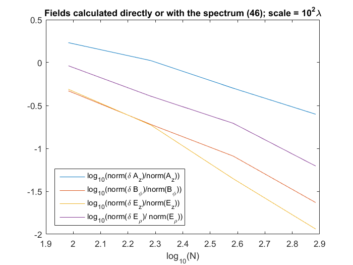
As expected,the errors (the relative delta’s on the different fields calculated either “directly” or “with the spectrum (46)”) decrease strongly as the discretization of the (here constant) spectrum function $S(k)$ becomes finer, i.e., with increasing $N$. (See Eq. (28).) This validates the correctness of our calculations. However, the errors increase quickly when the scale length $\verb+scale+$ is increased (even though it remains here enormously smaller than the galactic scale). This is because the integrals in Eqs. (22) and (13)–(15) involve functions of $k$ that oscillate with a frequency or a pseudo-frequency which is proportional to the magnitude of the spatial variables $\rho$ and $z$. As these integrals are approximated by the discrete sums (34) and (39)–(41), one would have to increase the discretization number $N$ in proportion of the scale length $\verb+scale+$.

In addition to this validation test, which does test our programs but is based on the “unphysical” solution (18), we will also compare the outcome of Eqs. (39)–(41) with the exact solution that corresponds to a set of spherical sources situated at the points ${\bf x}_{i}$. That is, one defines an exact solution of the source-free Maxwell equations by summing solutions obtained by Eqs. (4)–(6) applied to the outgoing spherical wave (19). That sum is similar to the sum $\Psi_{({\bf x}_{i})\ (\omega_{j})\ (S^{\prime}_{j})}$ given by Eq. (20). (Thus, all sources have the same amplitude and the same frequency spectrum, but this can easily be changed.) The fields produced by the individual source at ${\bf x}_{i}$ are denoted by $B_{\phi\,i}$, $E_{\rho\,i}$ and $E_{z\,i}$. In the case of a single frequency $\omega$, one first applies Eqs. (4)–(6) with $A_{z}=\psi^{\prime}_{\omega}$ as given by Eq. (19):

$$B_{\phi\omega}(t,\rho,z)=\frac{\rho}{r^{2}}\left(\sin\varphi+\frac{\cos\varphi}{Kr}\right),\qquad\varphi:=Kr-\omega t,$$

(47)

$$E_{\rho\omega}(t,\rho,z)=\frac{c^{2}}{\omega}\frac{\rho z}{r^{3}}\left[3\frac{\cos\varphi}{r}+\left(K-\frac{3}{Kr^{2}}\right)\sin\varphi\right],$$

(48)

$$E_{z\omega}(t,\rho,z)=\frac{c^{2}}{\omega r}\left[\left(\frac{3z^{2}}{r^{2}}-1\right)\frac{\cos\varphi}{r}+\left(-\frac{3z^{2}}{Kr^{3}}+\frac{1+K^{2}z^{2}}{Kr}-Kr\right)\frac{\sin\varphi}{r}\right],$$

(49)

but with $\rho$, $z$ and $r$ being replaced by

$$\rho^{\prime}_{i}:=\sqrt{(x-x_{i})^{2}+(y-y_{i})^{2}},$$

(50)

$$Z_{i}:=z-z_{i},$$

(51)

$$r_{i}:=\left|{\bf x}-{\bf x}_{i}\right|=\sqrt{(x-x_{i})^{2}+(y-y_{i})^{2}+(z-z_{i})^{2}}=\sqrt{\rho^{\prime 2}_{i}+Z_{i}^{2}}.$$

(52)

The definition of $B_{\phi\,i}$, $E_{\rho\,i}$ and $E_{z\,i}$ is that the exact fields produced at ${\bf x}$ by the source at ${\bf x}_{i}$ are decomposed on the orthonormal direct basis made of

$${\bf e}^{\prime}_{\rho\,i}={\bf e}^{\prime}_{\rho}({\bf x};{\bf x}_{i})=\left((x-x_{i}){\bf e}_{x}+(y-y_{i}){\bf e}_{y}\right)/\rho^{\prime}_{i},$$

(53)

$${\bf e}^{\prime}_{\phi\,i}={\bf e}^{\prime}_{\phi}({\bf x};{\bf x}_{i}):={\bf e}_{z}\wedge{\bf e}^{\prime}_{\rho}({\bf x};{\bf x}_{i})=\left((x-x_{i}){\bf e}_{y}-(y-y_{i}){\bf e}_{x}\right)/\rho^{\prime}_{i},$$

(54)

and ${\bf e}_{z}$. When each spherical source has the same finite frequency spectrum $(\omega_{j},S^{\prime}_{j})$, as in Eq. (20), it is understood that the components $B_{\phi\,i}$, $E_{\rho\,i}$ and $E_{z\,i}$ involve the corresponding weighted sum, e.g.

$$B_{\phi\,i}=\sum_{j=1}^{N_{\omega}}S^{\prime}_{j}\ B_{\phi\,i\,{\omega_{j}}},$$

(55)

where $B_{\phi\,i\,{\omega_{j}}}$ is given by Eq. (47) with $\rho^{\prime}_{i},Z_{i},r_{i},\omega_{j},K_{j}$ in the place of $\rho,z,r,\omega,K$. The total exact fields, sums of these different fields, are (reminding that $B_{\rho\,i}=B_{z\,i}=E_{\phi\,i}=0$):

$$B_{\phi}:={\bf B.e}_{\phi}=\sum_{i}B_{\phi\,i}\,{\bf e}^{\prime}_{\phi\,i}{\bf.e}_{\phi},$$

(56)

$$E_{\rho}:={\bf E.e}_{\rho}=\sum_{i}E_{\rho\,i}\,{\bf e}^{\prime}_{\rho\,i}{\bf.e}_{\rho},$$

(57)

$$E_{z}:={\bf E.e}_{z}=\sum_{i}E_{z\,i}.$$

(58)

In general, the other components of the total fields may be non-zero also, but we assume that the distribution of the identical spherical sources is axisymmetric (see Sect 2.2). In that case, we expect that $E_{\phi}=B_{\rho}=B_{z}=0$. Note also that ${\bf e}_{\rho}$ and ${\bf e}_{\phi}$, hence also the scalar products in Eqs. (56)–(57), and therefore also the $B_{\phi}$ and $E_{\rho}$ components, are not defined if $\rho=0$.

References

- [1] Beck R, Wielebinski R. Magnetic fields in the Milky Way and in galaxies. In: Planets, Stars and Stellar Systems. Oswalt TD, Gilmore G, editors, vol. 5, Dordrecht: Springer, 2013, pp. 641–723
- [2] Chamandy L, Subramanian K, Shukurov A. Galactic spiral patterns and dynamo action I: a new twist on magnetic arms. Mon. Not. R. Astron. Soc. 2013;428:3569–3589.
- [3] Porter TA, Strong AW. A new estimate of the galactic interstellar radiation field between m and m. In: Proc. 29th International Cosmic Ray Conference, Pune. Mumbai: Tata Institute of Fundamental Research; 2005; Vol. 4, pp. 77-80.
- [4] Maciel WJ. The interstellar radiation field. In: Astrophysics of the interstellar medium. Maciel WJ, editor. New York: Springer; 2013; Chapter 2, pp. 17-31.
- [5] Arminjon M. On the equations of electrodynamics in a flat or a curved spacetime and a possible interaction energy. Open Physics 2018;16:488–498.
- [6] Arminjon M. Interaction energy of a charged medium and its EM field in a curved spacetime. In: Geometry, integrability and quantization XX; Mladenov IM, Pulov V, Yoshioka A, editors, Sofia: Avangard Prima; 2019; pp. 88-98.
- [7] Arminjon M. Continuum dynamics and the electromagnetic field in the scalar ether theory of gravitation. Open Physics 2016;14:395–409.
- [8] Kent SM, Dame TM, Fazio G. Galactic structure from the Spacelab infrared telescope. II. Luminosity models of the Milky Way. Astroph. J. 1991;378:131–138.
- [9] Robin AC, Crézé M, Mohan V. The radial structure of the Galactic disc. Astron. Astrophys. 1992;265:32–39.
- [10] Porcel C, Garzón F, Jiménez-Vicente J. The radial scale length of the Milky Way. Astron. Astrophys. 1998;330:136–138.
- [11] Schneider P. Extragalactic astronomy and cosmology: an introduction. Berlin: Springer; p. 55.
- [12] Zamboni-Rached M, Recami E, Hernández-Figueroa H E. Structure of nondiffracting waves and some interesting applications. In: Localized waves; Hernández-Figueroa HE, Zamboni-Rached, Recami E, editors. Localized waves. Hoboken: John Wiley & Sons; 2008; pp. 43–77.
- [13] Garay-Avendaño RL, Zamboni-Rached M. Exact analytic solutions of Maxwell’s equations describing propagating nonparaxial electromagnetic beams. Appl. Opt. 2014;53:4524–4531.
- [14] Arminjon M. An explicit representation for the axisymmetric solutions of the free Maxwell equations. Open Physics 2020;18:255–263.
- [15] Jackson JD. Classical electrodynamics. 3rd ed. Hoboken: John Wiley & Sons; 1998; p. 360.
- [16] Durnin J. Exact solutions for nondiffracting beams. I. The scalar theory. J. Opt. Soc. Am. A 1987;4:651–654.
- [17] Gradshteyn IS, Ryzhik IM. Table of Integrals, Series, and Products. 7th English Edition. Burlington (Mass., USA): Academic Press; 2007; §6.677, p. 722.
- [18] Ala G, Francomano E, Viola F. A wavelet operator on the interval in solving Maxwell’s equations. Prog. Electromag. Res. Lett. 2011;27:133–140.
- [19] Atkinson KE. An Introduction to Numerical Analysis. 2nd Edition. New York: John Wiley & Sons; 1989; pp. 257–258.