Effects of gas temperature on Monte-Carlo simulations of charged particles drift in gaseous mediumJournal: J. Phys. D: Appl. Phys.

Michele Renda Iulia Stefania Trandafir Email: michele.renda@cern.ch Affiliation: Faculty of Physics, University of Bucharest - Măgurele, Romania

Abstract

We present the derivation of kinetic formulas modeling the microscopic interaction of a charged particle withing a molecular gas under effect of thermal motion. Both elastic and inelastic processes are taken in account. The results were verified to reproduce the non-thermal formulas when the target molecule velocity is set to zero. A set of simulation is provided to highlight the effects in Argon and Carbon tetrafluoride. Our results can applied in Monte-Carlo simulation of particle drift at energies of the same order of the thermal kinetic energy of the buffer gas.

1 Introduction

Monte-Carlo simulations have an important role in the calculation of the swarm coefficients of electrons and ions drifting in gaseous medium under the effect of an electromagnetic field. Historically, such calculations were performed thus the resolution of the Boltzmann transport equation [1, 2] and this method is still used today when the predominant class of collisions is composed by elastic processes.

However, thanks to the advance of computing technology, it is possible to solve these problems using methods which perform a microscopic simulation of a large number of interactions and then perform a statistical analysis to extract macroscopic attributes of the system. The main advantage of this approach is that we can better simulate the inelastic processes, such as ionization and excitation, being only limited by the computing power at our disposal.

Several software tools were developed to be able to simulate drift of charged particles, such as Magboltz [3] and METHES [4] (and their respective Cython and Python porting, PyBoltz [5] and pyMETHES [6]). Such tools are a valuable resource for the low pressure plasma community, being used for the simulation of gaseous detector used in high-energy physics experiments.

The authors of this article were involved also on the development of a software tools, Betaboltz [7], which uses some formulas discusses in this article to perform microscopic simulation of charged particle in gaseous medium.

The simulation of microscopic collisions is not a complex processes and can be divided in four elementary steps:

1.

Calculation of the free path for each charged particle.
2.

Chose of the interaction process (elastic, inelastic, etc.).
3.

Determination of the new particle direction.
4.

Determination of the energy transfer.

Because these steps must be repeated thousands of times, it is critical that they should be implemented as efficient as possible. The first step can be performed using the null-collision technique as described by Skullerud [8] and improved by Lin and Bardsley [9], Brennan [10] and Koura [11].

Once the free path was chosen for the current particle, and confirmed it is a not null collision, we have to select the physics process that will take place. As shown by Fraser [12], we can perform a random selection, weighted on the process cross-section values seen by the particle at its current energy.

The last step consist on calculate the new direction of the particle and energy transfer. To proper choose a deflection angle, we can assume inelastic collision to be isotopic, while elastic collisions require the knowledge of the differential cross-section of the process. Unfortunately, such tables are quite rare and limited to a few common gases. However, it is possible to use integral cross-section tables, which are widely available in literature, to generate pseudo-differential cross-section tables using the methods presented by Okhrimovskyy et al. [13] or by Longo and Capitelli [14].

To calculate the energy transfer, we can use the formula presented by Fraser [12], which provides, for inelastic collisions, the following relation:

	$\displaystyle\Delta E_{1}=$	$\displaystyle\frac{m_{2}}{(m_{1}+m_{2})}\varepsilon_{k}/E_{1}-\frac{2m_{1}m_{2}}{(m_{1}+m_{2})^{2}}$			(1)
		$\displaystyle\left\{\left[1-\frac{(m_{1}+m_{2})}{m_{2}}\varepsilon_{k}/E_{1}\right]^{1/2}\cos\theta_{1}-1\right\}$			(1)

which, for elastic collisions, reduces to:

\Delta E_{1}=\frac{2m_{1}m_{2}(1-\cos\theta_{1})}{(m_{1}+m_{2})^{2}}

(2)

Here, $m_{1}$ is the mass of the charged particle, an electron or ion, named bullet, $m_{2}$ is the mass of the gas molecule, from now on label as target, $E_{1}$ is the bullet energy, $\theta_{1}$ is the deflection angle in center of momentum frame (more on this in next section) and $\varepsilon_{k}$ the threshold energy of the inelastic process.

Analyzing (1) and (2), we may notice there is no reference about the target molecule energy but only to its mass. The reason is that the target molecule is considered at rest. This approximation holds well for the energy domain in common particle drift experiments. However, when the drift fields goes below $\approx$ $0.01\text{\,}\mathrm{Td}$ , the mean energy for an electron became comparable to the thermal energies of the gas molecules ( $\approx$ $25\text{\,}\mathrm{meV}$ at standard conditions).

In this article, we will derive and discuss how (1) and (2) were derived, and we will provide a set of equations which can be used to get a more precise simulation at low reduced fields.

2 Conventions and reference frames

When discussing microscopic collisions between a charged particle and a molecule, it is important to define the right frame of reference. In an experimental setup, it is commonly used the laboratory frame of reference. However, when handling collisions between two moving objects, it is easier to work in the center-of-momentum reference frame. Indeed, we can define, three reference frames:

1.

Global laboratory reference frame
2.

Local laboratory reference frame
3.

Center-of-momentum reference frame

The first one, is the normal reference frame which is arbitrary aligned, usually with one of its axis is a relevant axis of the experimental setup. The second one, is just a rotation of the first reference frame, such as the $z$ -axis will be aligned along the velocity of the bullet particle. The last one, will be relative to the center-of-momentum frame, defined as:

\textbf{V}_{cm}=\frac{m_{1}\textbf{V}_{1}+m_{2}\textbf{V}_{2}}{m_{1}+m_{2}}

(3)

where, $m_{1}$ and $m_{2}$ are the bullet and target mass, and $\textbf{V}_{1}$ , $\textbf{V}_{2}$ their velocities. We think it is important to remark that, while the global laboratory reference frame is static during the simulation, the other two frames are different for each collision. In this article we will ignore the global laboratory frame, and we will focus only on the local laboratory and the center-of-momentum frame (shown respectively in figure 1 and 2).

Refer to caption — Figure 1: In this frame, the $z$ -axis is aligned along $\textbf{V}_{1}$ , while $\textbf{V}_{2}$ falls in the $xz$ -plane. $\textbf{V}_{cm}$ is not null and can be calculated using (3).

In the remaining part of the article, we will use these conventions:

•

Capital symbols will be used for laboratory frame quantities
•

Lowercase symbols will be used for center-of-momentum frame quantities
•

Bold symbols refer to Cartesian vectors
•

The lower script 1 will be used for the bullet, the electron or ion which is drifter by the electromagnetic field.
•

The lower script 2 will be used for the target, gas molecules which may have thermal kinetic energies.
•

The apostrophe will be used to mark after-collisions quantities, while plain symbols will be used for before-collsion quantities or constant attributes such as masses.

3 Particle collisions in center of momentum frame

In the center-of-momentum frame, we can threat the collisions with the common conservation laws, keeping in mind that, due to how this frame is defined, the total moment of the system is zero:

	$\displaystyle m_{1}\textbf{v}_{1}+m_{2}\textbf{v}_{2}=0$		(4)
	$\displaystyle m_{1}\textbf{v}_{1}^{\prime}+m_{2}\textbf{v}_{2}^{\prime}=0$		(5)
	$\displaystyle\frac{1}{2}m_{1}(v_{1})^{2}+\frac{1}{2}m_{2}(v_{2})^{2}=\frac{1}{2}m_{1}(v_{1}^{\prime})^{2}+\frac{1}{2}m_{2}(v_{2}^{\prime})^{2}+\varepsilon_{k}$		(6)

Combining (4) and (5), we get the relations:

\textbf{v}_{2}=-\frac{m_{1}}{m_{2}}\textbf{v}_{1}\\ \textbf{v}_{2}^{\prime}=-\frac{m_{1}}{m_{2}}\textbf{v}_{1}^{\prime}\\

(7)

and using (6):

	$\displaystyle v_{1}^{\prime}=\sqrt{v^{2}_{1}-\frac{2m_{2}}{m^{2}_{1}+m_{1}m_{2}}\varepsilon_{k}}$		(8)
	$\displaystyle v_{2}^{\prime}=\sqrt{v^{2}_{2}-\frac{2m_{1}}{m^{2}_{2}+m_{1}m_{2}}\varepsilon_{k}}$		(9)
	$\displaystyle\varepsilon_{1}^{\prime}=\varepsilon_{1}-\frac{m_{2}}{m_{1}+m_{2}}\varepsilon_{k}$		(10)
	$\displaystyle\varepsilon_{2}^{\prime}=\varepsilon_{2}-\frac{m_{1}}{m_{1}+m_{2}}\varepsilon_{k}$		(11)

4 Energy transfer in laboratory frame

Moving from the laboratory frame to the center-of-momentum frame, can be done using the relations:

	$\displaystyle\textbf{v}_{1}$	$\displaystyle=\textbf{V}_{1}-\textbf{V}_{cm}$			(12)
	$\displaystyle\textbf{v}_{2}$	$\displaystyle=\textbf{V}_{2}-\textbf{V}_{cm}$			(13)

and vice-versa:

	$\displaystyle\textbf{V}_{1}^{\prime}$	$\displaystyle=\textbf{V}_{cm}+\textbf{v}_{1}^{\prime}$			(14)
	$\displaystyle\textbf{V}_{2}^{\prime}$	$\displaystyle=\textbf{V}_{cm}+\textbf{v}_{2}^{\prime}$			(15)

To get the final velocities, we can replace (8), (9) in (14) and (15):

	$\displaystyle\textbf{V}_{1}^{\prime}=\textbf{V}_{cm}+\sqrt{\|\textbf{V}_{1}-\textbf{V}_{cm}\|^{2}-\frac{2m_{2}}{m^{2}_{1}+m_{1}m_{2}}\varepsilon_{k}}\;\hat{\textbf{u}}_{1}^{\prime}$		(16)
	$\displaystyle\textbf{V}_{2}^{\prime}=\textbf{V}_{cm}+\sqrt{\|\textbf{V}_{2}-\textbf{V}_{cm}\|^{2}-\frac{2m_{1}}{m^{2}_{2}+m_{1}m_{2}}\varepsilon_{k}}\;\hat{\textbf{u}}_{2}^{\prime}$		(17)

where $\hat{\textbf{u}}_{1}^{\prime}=\textbf{v}_{1}^{\prime}/v_{1}^{\prime}$ and $\hat{\textbf{u}}_{2}^{\prime}=\textbf{v}_{2}^{\prime}/v_{2}^{\prime}$ are the unitary velocity vectors. Then we can use (3):

$\displaystyle\textbf{V}_{1}^{\prime}$	$\displaystyle=\frac{m_{1}\textbf{V}_{1}+m_{2}\textbf{V}_{2}}{m_{1}+m_{2}}\cdot\hat{\textbf{U}}_{cm}$	(18)
	$\displaystyle+\frac{m_{2}}{m_{1}+m_{2}}\sqrt{\|\textbf{V}_{1}-\textbf{V}_{2}\|^{2}-\frac{2(m_{1}+m_{2})}{m_{1}m_{2}}\varepsilon_{k}}\;\hat{\textbf{u}}_{1}^{\prime}$	(18)
$\displaystyle\textbf{V}_{2}^{\prime}$	$\displaystyle=\frac{m_{1}\textbf{V}_{1}+m_{2}\textbf{V}_{2}}{m_{1}+m_{2}}\cdot\hat{\textbf{U}}_{cm}$	(19)
	$\displaystyle+\frac{m_{1}}{m_{1}+m_{2}}\sqrt{\|\textbf{V}_{2}-\textbf{V}_{1}\|^{2}-\frac{2(m_{1}+m_{2})}{m_{1}m_{2}}\varepsilon_{k}}\;\hat{\textbf{u}}_{2}^{\prime}$	(19)

to calculate particle energies:

	$\displaystyle E_{1}^{\prime}=\frac{1}{2}m_{1}\left\|\frac{m_{1}V_{1}+m_{2}V_{2}}{m_{1}+m_{2}}\;\hat{\textbf{U}}_{cm}+\frac{m_{2}}{m_{1}+m_{2}}\right.$		(20)
	$\displaystyle\left.\sqrt{V^{2}_{1}+V^{2}_{2}-2V_{1}V_{2}\cos\Theta_{2}-\frac{2(m_{1}+m_{2})}{m_{1}m_{2}}\varepsilon_{k}}\;\hat{\textbf{u}}_{1}^{\prime}\right\|^{2}$
	$\displaystyle E_{2}^{\prime}=\frac{1}{2}m_{2}\left\|\frac{m_{1}V_{1}+m_{2}V_{2}}{m_{1}+m_{2}}\;\hat{\textbf{U}}_{cm}+\frac{m_{1}}{m_{1}+m_{2}}\right.$		(21)
	$\displaystyle\left.\sqrt{V^{2}_{2}+V^{2}_{1}-2V_{2}V_{1}\cos\Theta_{2}-\frac{2(m_{1}+m_{2})}{m_{1}m_{2}}\varepsilon_{k}}\;\hat{\textbf{u}}_{2}^{\prime}\right\|^{2}$

where $\hat{\textbf{U}}_{cm}$ is the center of momentum unit vector:

$\displaystyle\textbf{V}_{cm}$	$\displaystyle=\frac{m_{1}V_{1}(0,0,1)+m_{2}V_{2}(\sin\Theta_{2},0,\cos\Theta_{2})}{m_{1}+m2}$	(22)
	$\displaystyle=\frac{m_{2}V_{2}}{m_{1}+m2}\;\;(\sin\Theta_{2},0,\cos\Theta_{2}+\frac{m_{1}V_{1}}{m_{2}V_{2}})$	(22)
$\displaystyle\Gamma$	$\displaystyle=\sqrt{1+\left(\frac{m_{1}V_{1}}{m_{2}V_{2}}\right)^{2}+2\frac{m_{1}V_{1}}{m_{2}V_{2}}\cos\Theta_{2}}$	(23)
$\displaystyle\hat{\textbf{U}}_{cm}$	$\displaystyle=\frac{\textbf{V}_{cm}}{V_{cm}}=(\sin\Theta_{2},0,\cos\Theta_{2}+\frac{m_{1}V_{1}}{m_{2}V_{2}})/\Gamma$	(24)

Here we can define the quantity:

\displaystyle\Delta

\displaystyle=\sqrt{V^{2}_{1}+V^{2}_{2}-2V_{1}V_{2}\cos\Theta_{2}-\frac{2(m_{1}+m_{2})}{m_{1}m_{2}}\varepsilon_{k}}

(25)

leading us to the vectorial relation:

	$\displaystyle E_{1}^{\prime}$	$\displaystyle=\frac{1}{2}m_{1}\left\|\frac{m_{1}V_{1}+m_{2}V_{2}}{m_{1}+m_{2}}\;\hat{\textbf{U}}_{cm}+\frac{m_{2}}{m_{1}+m_{2}}\Delta\;\hat{\textbf{u}}_{1}^{\prime}\right\|^{2}$			(26)
	$\displaystyle E_{2}^{\prime}$	$\displaystyle=\frac{1}{2}m_{2}\left\|\frac{m_{1}V_{1}+m_{2}V_{2}}{m_{1}+m_{2}}\;\hat{\textbf{U}}_{cm}+\frac{m_{1}}{m_{1}+m_{2}}\Delta\;\hat{\textbf{u}}_{2}^{\prime}\right\|^{2}$			(27)

or, the scalar form:

$\displaystyle E_{1}^{\prime}=\frac{1}{2}m_{1}$	$\displaystyle\left[\left(\frac{m_{1}V_{1}+m_{2}V_{2}}{m_{1}+m_{2}}\right)^{2}+\left(\frac{m_{2}\Delta}{m_{1}+m_{2}}\right)^{2}\right.$	(28)
	$\displaystyle\qquad+\left.\frac{2m_{2}\Delta\Omega_{1}(m_{1}V_{1}+m_{2}V_{2})}{\left(m_{1}+m_{2}\right)^{2}}\right]$	(28)
$\displaystyle E_{2}^{\prime}=\frac{1}{2}m_{2}$	$\displaystyle\left[\left(\frac{m_{1}V_{1}+m_{2}V_{2}}{m_{1}+m_{2}}\right)^{2}+\left(\frac{m_{1}\Delta}{m_{1}+m_{2}}\right)^{2}\right.$	(29)
	$\displaystyle\qquad+\left.\frac{2m_{1}\Delta\Omega_{2}(m_{1}V_{1}+m_{2}V_{2})}{\left(m_{1}+m_{2}\right)^{2}}\right]$	(29)

given we define the cosine between $\hat{\textbf{U}}_{cm}$ and $\hat{\textbf{u}}^{\prime}$ as:

	$\displaystyle\Omega_{1}=\hat{\textbf{U}}_{cm}\cdot\hat{\textbf{u}}_{1}=$		(30)
	$\displaystyle\left(\sin\Theta_{2}\sin\theta^{\prime}_{1}\cos\phi_{1}^{\prime}+\cos\Theta_{2}\cos\theta_{1}^{\prime}+\frac{m_{1}V_{1}}{m_{2}V_{2}}\cos\theta_{1}^{\prime}\right)/\Gamma$
	$\displaystyle\Omega_{2}=\hat{\textbf{U}}_{cm}\cdot\hat{\textbf{u}}_{2}=$		(31)
	$\displaystyle\left(\sin\Theta_{2}\sin\theta^{\prime}_{2}\cos\phi_{2}^{\prime}+\cos\Theta_{2}\cos\theta_{2}^{\prime}+\frac{m_{1}V_{1}}{m_{2}V_{2}}\cos\theta_{2}^{\prime}\right)/\Gamma$

5 Specific case: $V_{2}=0$ and $\varepsilon_{k}=0$

The simplest verification is to check if we get back to (2) for elastic collisions ( $\varepsilon_{k}=0$ ) where the bullet energy is greater than the thermal gas energy ( $V_{1}\gg V_{2}$ ). In this case, we get a finite value for (25)

\displaystyle\Delta

\displaystyle=V_{1}

(32)

and an infinite value for (23):

\displaystyle\Gamma\rightarrow\infty

(33)

However, we can calculate the limits getting:

	$\displaystyle\lim\limits_{V_{2}\rightarrow 0}\Omega_{1}=\cos\theta_{1}^{\prime}$		(34)
	$\displaystyle\lim\limits_{V_{2}\rightarrow 0}\Omega_{2}=\cos\theta_{2}^{\prime}$		(35)

allowing reducing (28) and (29) to:

	$\displaystyle E_{1}^{\prime}=\frac{1}{2}m_{1}$	$\displaystyle\left[\frac{m^{2}_{1}+m^{2}_{2}+2m_{1}m_{2}\cos\theta_{1}^{\prime}}{\left(m_{1}+m_{2}\right)^{2}}\right]V^{2}_{1}$			(36)
	$\displaystyle E_{2}^{\prime}=\frac{1}{2}m_{2}$	$\displaystyle\left[\frac{2m^{2}_{1}(1+\cos\theta_{2}^{\prime})}{\left(m_{1}+m_{2}\right)^{2}}\right]V^{2}_{1}$			(37)

and finally, defining $\Delta E=E-E^{\prime}$ , to:

	$\displaystyle\Delta E_{1}^{\prime}=$	$\displaystyle\frac{2m_{1}m_{2}(1-\cos\theta_{1}^{\prime})}{\left(m_{1}+m_{2}\right)^{2}}E_{1}$			(38)
	$\displaystyle\Delta E_{2}^{\prime}=-$	$\displaystyle\frac{2m_{1}m_{2}(1+\cos\theta_{2}^{\prime})}{\left(m_{1}+m_{2}\right)^{2}}E_{1}$			(39)

6 Specific case: $V_{2}=0$ and $\varepsilon_{k}\neq 0$

For inelastic collisions ( $\varepsilon_{k}\neq 0$ ), we can replace in (28) and (29) the values $V_{1}=\sqrt{2E_{1}/m_{1}}$ and $V_{2}=0$ . In this way we get:

	$\displaystyle\Delta=\sqrt{\frac{2m_{2}E_{1}-2(m_{1}+m_{2})\varepsilon_{k}}{m_{1}m_{2}}}$		(40)
	$\displaystyle\lim\limits_{V_{2}\rightarrow 0}\Omega_{1}=\cos\theta_{1}^{\prime}$		(41)
	$\displaystyle\lim\limits_{V_{2}\rightarrow 0}\Omega_{2}=\cos\theta_{2}^{\prime}$		(42)

and finally:

$\displaystyle E_{1}^{\prime}=$	$\displaystyle\left[1-\frac{m_{2}}{m_{1}+m_{2}}\frac{\varepsilon_{k}}{E_{1}}+\right.$	(43)
	$\displaystyle\left.\frac{2m_{1}m_{2}}{(m_{1}+m_{2})^{2}}\left(\sqrt{1-\frac{m_{1}+m_{2}}{m_{2}}\frac{\varepsilon_{k}}{E_{1}}}\cos\theta_{1}^{\prime}-1\right)\right]E_{1}$	(43)
$\displaystyle E_{2}^{\prime}=$	$\displaystyle\frac{2m_{1}m_{2}}{(m_{1}+m_{2})^{2}}\left[1-\frac{m_{1}+m_{2}}{2m_{2}}\frac{\varepsilon_{k}}{E_{1}}+\right.$	(44)
	$\displaystyle\left.\sqrt{1-\frac{m_{1}+m_{2}}{m_{2}}\frac{\varepsilon_{k}}{E_{1}}}\cos\theta_{2}^{\prime}\right]E_{1}$	(44)

7 Plots

In this section, we present the Monte-Carlo simulation of the drift of electrons in a uniform static electric field. To perform the simulation, we used a framework we developed [7, 15, 16]. A total of $25$ particles were put in an infinite volume under the effect of a static uniform electric field between $1\text{\times}{10}^{-3}\text{\,}\mathrm{Td}1\text{\times}{10}^{-1}\text{\,}\mathrm{Td}$ .

The collision time were calculated using the null-collision technique and the null-collision technique [8] while, for the collision kinematics, we used the relations provided by Okhrimovskyy [13]. The simulation if stopped when reaching $250\,000$ real collisions and, the whole event, is repeated $250$ times for each field value.

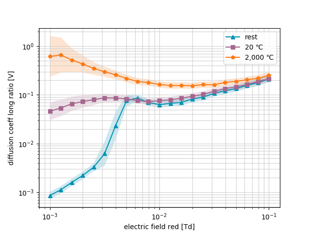
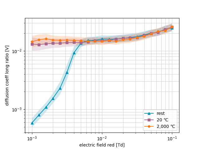
First we performed a simulation at $0\text{\,}\mathrm{K}$ temperature, where all the gas components are at rest and does not have any kinetic energy. Then we repeated the simulation at $20\text{\,}\mathrm{\SIUnitSymbolCelsius}$ and at $2000\text{\,}\mathrm{\SIUnitSymbolCelsius}$ , to confirm the behavior for increasing temperatures.

In figure 3, we can see the simulated drift velocities for a mono-atomic molecule and for a poly-atomic gas with spherical symmetry. We can notice that for higher electric fields, the drift velocities tends to converge. This is expected, because in this region, the mean electron energy is bigger than the thermal energy of the gas components.

In figure 4, we can see how, for lower fields, the gas temperature has a direct impact on the diffusion coefficients: the electrons are spread out by the chaotic thermal movement of the gas molecules.

8 Conclusions

In this article, we presented our derivation of kinematic formulas to describe electron or ion collisions in gaseous medium at low electric fields, where gas molecules can not be considered at rest. We consider these relations to be useful when performing Monte-Carlo simulation at low $E/N$ values.

CRediT author statement

Michele Renda: Conceptualization, Methodology, Software, Writing - Original Draft
Iulia Stefania Trandafir: Writing-Reviewing and Editing, Formal analysis, Validation

This work was supported by the research grants ATLAS CERN-RO and PN19060104.

References

[1] Boltzmann L 1896 Vorlesungen über gastheorie vol 1 (JA Barth)
[2] Ness K F 1994 Journal of Physics D: Applied Physics 27 1848 ISSN 0022-3727 URL http://stacks.iop.org/0022-3727/27/i=9/a=007
[3] Biagi S F 1999 Nuclear Instruments and Methods A421 234–240
[4] Rabie M and Franck C M 203 268–277 ISSN 0010-4655 URL http://www.sciencedirect.com/science/article/pii/S0010465516300376
[5] Al Atoum B, Biagi S F, González-Díaz D, Jones B J P and McDonald A D 254 107357 ISSN 0010-4655 URL http://www.sciencedirect.com/science/article/pii/S0010465520301533
[6] Chachereau A pymethes gitlab page URL https://gitlab.com/ethz_hvl/pymethes
[7] Renda M and Ciubotaru D A Betaboltz: a monte-carlo simulation tool for gas scattering processes URL https://arxiv.org/abs/1901.08140
[8] Skullerud H R 1968 Journal of Physics D: Applied Physics 1 1567 ISSN 0022-3727 URL http://stacks.iop.org/0022-3727/1/i=11/a=423
[9] Lin S L and Bardsley J N 66 435–445 ISSN 0021-9606 URL http://aip.scitation.org/doi/abs/10.1063/1.433988
[10] Brennan M J 19 256–261 ISSN 1939-9375 conference Name: IEEE Transactions on Plasma Science
[11] Koura K 35 139–154 ISSN 0898-1221 URL http://www.sciencedirect.com/science/article/pii/S0898122197002642
[12] Fraser G W and Mathieson E 257 339–345 ISSN 0168-9002 URL http://www.sciencedirect.com/science/article/pii/0168900287907558
[13] Okhrimovskyy A, Bogaerts A and Gijbels R 65 037402 publisher: American Physical Society URL https://link.aps.org/doi/10.1103/PhysRevE.65.037402
[14] Longo S and Capitelli M 14 1–13 ISSN 0272-4324, 1572-8986 URL https://link.springer.com/article/10.1007/BF01448734
[15] Renda M Betaboltz gitlab URL https://gitlab.com/micrenda/betaboltz
[16] Renda M Drifter gitlab URL https://gitlab.com/micrenda/drifter
[17] Biagi (transcription of data from sf biagi’s fortran code, magboltz.), retrived on 28 oct 2019, www.lxcat.net URL http://www.lxcat.net/contributors/#d6
[18] Bsr (quantum-mechanical calculations by o. zatsarinny and k. bartschat), retrived on 29 may 2020, www.lxcat.net URL http://www.lxcat.net/contributors/#d2
[19] Bordage database, retrived on 08 apr 2019, www.lxcat.net URL http://www.lxcat.net/contributors/#d7

	$\displaystyle E_{1}^{\prime}=\frac{1}{2}m_{1}\left\|\frac{m_{1}V_{1}+m_{2}V_{2}}{m_{1}+m_{2}}\;\hat{\textbf{U}}_{cm}+\frac{m_{2}}{m_{1}+m_{2}}\right.$		(20)
	$\displaystyle\left.\sqrt{V^{2}_{1}+V^{2}_{2}-2V_{1}V_{2}\cos\Theta_{2}-\frac{2(m_{1}+m_{2})}{m_{1}m_{2}}\varepsilon_{k}}\;\hat{\textbf{u}}_{1}^{\prime}\right\|^{2}$
	$\displaystyle E_{2}^{\prime}=\frac{1}{2}m_{2}\left\|\frac{m_{1}V_{1}+m_{2}V_{2}}{m_{1}+m_{2}}\;\hat{\textbf{U}}_{cm}+\frac{m_{1}}{m_{1}+m_{2}}\right.$		(21)
	$\displaystyle\left.\sqrt{V^{2}_{2}+V^{2}_{1}-2V_{2}V_{1}\cos\Theta_{2}-\frac{2(m_{1}+m_{2})}{m_{1}m_{2}}\varepsilon_{k}}\;\hat{\textbf{u}}_{2}^{\prime}\right\|^{2}$

Effects of gas temperature on Monte-Carlo simulations of charged particles drift in gaseous mediumJournal: J. Phys. D: Appl. Phys.

Abstract

1 Introduction

2 Conventions and reference frames

3 Particle collisions in center of momentum frame

4 Energy transfer in laboratory frame

5 Specific case: V2=0V_{2}=0 and εk=0\varepsilon_{k}=0

6 Specific case: V2=0V_{2}=0 and εk≠0\varepsilon_{k}\neq 0

7 Plots

8 Conclusions

CRediT author statement

References

References

5 Specific case: $V_{2}=0$ and $\varepsilon_{k}=0$

6 Specific case: $V_{2}=0$ and $\varepsilon_{k}\neq 0$