Quantum Speedup of Natural Gradient for Variational Bayes

One of the most promising classical advances in VB is the use of natural gradient instead of Euclidean gradient in stochastic gradient descent (Amari 1998; Sato 2001; Tran et al. 2017; Mishkin et al. 2018). Being a geometric object that takes into account the information geometry of the variational family, natural gradient often leads to faster and more stable convergence than alternative methods Martens 2020. In situations where variational parameters lie on Riemannian manifolds, natural gradient is the only reliable adaptive learning method that speeds up VB training Tran et al. 2021a. However, in many cases, accurate computation of natural gradient is infeasible, because it requires the analytic computation and inversion of the Fisher information matrix. With computational complexity of $\tilde{O}(N^{d})$, with $2<d\leq 3$ depending on various algorithms ($d=3$ in practice), natural gradient estimation is prohibitively computationally expensive in high-dimensional cases; current practice resorts to heuristic workarounds that can affect the results of Bayesian inference Martens and Grosse 2015. We propose a regression-based approach to natural gradient estimation for VB, which lends itself to efficient computational methods, including quantum computing algorithms (Section III).

Let $y$ be the data and $L(\theta)=p(y|\theta)$ the likelihood function based on a statistical model, with $\theta$ the set of model parameters to be estimated. Let $p(\theta)$ be the prior. Bayesian inference encodes all information into the posterior distribution

The main task in Bayesian inference is to approximate the posterior $p(\theta|y)$, and VB does so by approximating it by a probability distribution with density $q_{\lambda}(\theta)$, $\lambda\in{\cal M}$ - the variational parameter space, belonging to some tractable family of distributions such as Gaussians or neural networks. Denote by $N$ the size of $\lambda$. The best $\lambda$ is found by maximizing the lower bound (Zhang et al. 2018)

with

The Euclidean gradient of the lower bound is (Tran et al. 2021b)

For maximizing the lower bound objective function $\mathcal{L}(\lambda)$, Amari Amari 1998 shows that the natural gradient, defined as

where

is the Fisher information matrix of $q_{\lambda}$, works much more efficiently than the Euclidean gradient. The reason is that the natural gradient takes into account the geometry of the variational family $\{q_{\lambda},\lambda\in{\cal M}\}$ in the optimization. Natural gradient has been proven vital to the success of VB; see, e.g., Refs. Sato 2001; Hoffman et al. 2013 among others.

The classical VB algorithm with the use of natural gradient proceeds as follows (Algorithm 1). Let $\widehat{\nabla_{\lambda}^{\text{nat}}{\mathcal{L}}}(\lambda)$ be an estimate of the natural gradient ${\nabla_{\lambda}^{\text{nat}}{\mathcal{L}}}(\lambda)$. At step $t$ of stochastic natural gradient descent, the natural gradient estimate is used to compute the momentum gradient $Y_{t+1}$, which in turn updates the variational parameter $\lambda_{t+1}=\lambda_{t}+\alpha_{t}Y_{t+1}$.

The momentum gradient method, found highly useful in practice, smooths out the natural gradient estimate as in (6) incorporating the latest estimate $\widehat{\nabla_{\lambda}^{\text{nat}}{\mathcal{L}}}(\lambda_{t})$ with the momentum weight $\omega\in(0,1)$. The learning rates $\alpha_{t}$ are required to satisfy: $1\geq\alpha_{t}\downarrow 0$, $\sum\alpha_{t}=\infty$ and $\sum\alpha_{t}^{2}<\infty$. We refer the interested reader to Ref. Tran et al. 2021b for more details.

The current practice of stochastic gradient descent for VB often includes gradient clipping that normalizes the length of $\widehat{\nabla_{\lambda}^{\text{nat}}{\mathcal{L}}}(\lambda_{t})$ Goodfellow et al. 2016.

The main computational bottleneck in Variational Bayes is computing the gradient estimate $\widehat{\nabla_{\lambda}^{\text{nat}}{\mathcal{L}}}(\lambda)$. We develop the regression-based natural gradient estimation method to overcome this problem, including with the use of a hybrid quantum-classical algorithm.

The obstacles to practical implementation of natural gradient descent are well-known. It is difficult to compute the Fisher matrix let alone its inverse. Even if one could compute the Fisher matrix analytically, solving the equation in (4) is computationally infeasible in high dimensions. Our regression-based approach to natural gradient estimation overcomes these difficulties.

Denote $T(\theta)=\nabla_{\lambda}\log q_{\lambda}(\theta)$, a vector-valued function often called the score function. By noting that ${\mathbb{E}}_{q_{\lambda}}(T(\theta))=0$, the Euclidean gradient of the lower bound in (3) and the Fisher matrix in (5) can be rewritten as

Hence, the natural gradient takes the form

Equation (9) invites the interpretation of the natural gradient as the slope vector $\beta$ of regression of the dependent variable $h_{\lambda}(\theta)$ on the vector of independent variables $T(\theta)$.

More concretely, let $\{\theta_{i}\}_{i=1}^{M}$ be $M$ samples from $q_{\lambda}(\theta)$, and consider the linear regression

where the $\epsilon_{i}$ are independently distributed with mean zero. We need an intercept $\beta_{0}$ in the regression model (10) because ${\mathbb{E}}_{q_{\lambda}}(T(\theta))=0$. We note that $\beta_{0}={\mathbb{E}}_{q_{\lambda}}(h_{\lambda}(\theta))=\mathcal{L}(\lambda)$; hence, an estimate of $\beta_{0}$ provides an estimate of the lower bound - an important quantity in the VB literature. Let $T$ be the design matrix whose row vectors are $(1,T(\theta_{i})^{\top})$ and $h$ be the response vector of $h_{\lambda}(\theta_{i})$. The minimum-norm ordinary least squares estimator of $(\beta_{0},{\beta}^{\top})^{\top}$ is

where $T^{+}$ denotes the pseudo-inverse of $T$ Kobak et al. 2020. When $M>N$, $g$ is the usual OLS estimator, $g=(T^{\top}T)^{-1}T^{\top}h$ and is an unbiased estimator of $(\beta_{0},{\beta}^{\top})^{\top}$. When $M<N$, $g=T^{\top}(TT^{\top})^{-1}h$ and is the minimum-norm solution to the underconstrained linear equation $Tg=h$, and it can be shown that $g$ is a consistent estimator (in $M$) of $(\beta_{0},{\beta}^{\top})^{\top}$.

In this paper, we focus mainly on the situation where the number of $\{\theta_{i}\}$ samples $M$ is much smaller than the number of parameters $N$, $M\ll N$. This is the situation observed in the vast majority of practical applications of VB in deep learning Liang et al. 2019; Bartlett et al. 2020; Dar et al. 2021.

Denote by $\widehat{\beta}$ the vector $g$ after deleting its very first component. We use $\widehat{\beta}$ as an estimator of the natural gradient $\nabla_{\lambda}^{\text{nat}}{\mathcal{L}}(\lambda)$. This regression-based natural gradient formulation is inspired by the method of Salimans and Knowles Salimans et al. 2013 and Malago et al. Malago et al. 2013 who consider a regression-based method for estimating the natural gradient when the variational distribution is limited to the exponential family. Our method is general and can be easily applied to situations with complicated variational distributions such as neural networks. Hereafter, for notational simplicity, we will refer to $g$ in (11) as the natural gradient estimator $\widehat{\nabla_{\lambda}^{\text{nat}}{\mathcal{L}}}(\lambda)$, although in practice one must remove the very first component of $g$ to obtain the natural gradient estimate.

The regression-based approach provides an estimate of the natural gradient that avoids the requirement to compute the Fisher matrix $I_{F}$ analytically. Pseudo-inversion of the short-and-wide $M\times N$, $M\ll N$ design matrix $T$ can be efficient. The time complexity of the popular Cholesky decomposition method is $\tilde{O}(NM^{2})$, scaling favorably with $N$, particularly if $M=O(N^{\alpha})$ with $0\leq\alpha<1/2$, where $\alpha=0$ denotes a polylogarithmic dependence on $N$. The method delivers significant efficiency over the naive methods to invert the $N\times N$ Fisher matrix, with time complexity of $\tilde{O}(N^{d})$, where $2<d\leq 3$ (and usually $d=3$ in practice). Note that the conjugate gradient method Shewchuk et al. 1994; Saad 2003, sometimes used as a classical benchmark for quantum linear systems algorithms Clader et al. 2013, does not apply to the natural gradient problem. The conjugate gradient method requires that the inverted matrix is symmetric and positive definite. The design matrix $T$ is not symmetric and its symmetrized version $\begin{pmatrix}0&T\\ T^{\dagger}&0\end{pmatrix}$ is not positive definite.

Theorem 1 in Section II.4 provides a convergence guarantee for VB optimization with natural gradient (Algorithm 1) under standard conditions.

This section provides a convergence analysis of the VB algorithm using the regression-based natural gradient described in the previous sections. To be consistent with the conventional notation in the optimization literature, let us denote $\tilde{\mathcal{L}}(\lambda):=-{\mathcal{L}}(\lambda)$ to be the objective function, the VB optimization problem becomes

Write the estimate $\widehat{\nabla_{\lambda}^{\text{nat}}\tilde{\mathcal{L}}}(\lambda_{t})$ of the natural gradient as

with $\epsilon_{t}$ the estimate error. In Algorithm 1, by viewing that the variational parameter $\lambda$ is updated first then the momentum gradient, it can be equivalently rewritten as:

For $t=0,1,...$

• •

  $\lambda_{t+1}=\lambda_{t}-Y_{t}$.

• •

  $Y_{t+1}=\zeta_{t+1}Y_{t}+\gamma_{t+1}(\nabla_{\lambda}^{\text{nat}}\tilde{\mathcal{L}}(\lambda_{t+1})+\epsilon_{t+1})$.

Here, $\zeta_{t}=\alpha_{t}\omega$ and $\gamma_{t}=\alpha_{t}(1-\omega)$ with $\omega$ the momentum weight and $\alpha_{t}$ the learning rates. For a symmetric and positive definite matrix $\Sigma$, we denote by $\sigma_{\max}(\Sigma)$, $\sigma_{\min}(\Sigma)$ the largest and smallest eigenvalue of $\Sigma$, and by $\|\cdot\|$ the $\ell^{2}$-norm.

The practical implication of condition (A3) is that, as the natural gradient estimate $\widehat{\nabla_{\lambda}^{\text{nat}}\tilde{\mathcal{L}}}(\lambda_{t})$ is no longer unbiased when $M<N$, it should be made more and more accurate along with iterations $t$. That is, one might need to gradually increase the sample size $M$ in the estimate (11). The result in (13) says that the algorithm does stop at a stationary point of the target $\tilde{\mathcal{L}}(\lambda)$. The result in (14) says that, under the strong convexity condition, the algorithm converges to the minimum point $\lambda^{*}$. The proof can be found in the Appendix.

Amari Amari 1998 demonstrated that (non-stochastic) natural gradient is Fisher-efficient and, since Amari’s work was published, natural gradient has been shown to require far fewer iterations than other methods for many models (see, e.g., Ref. Martens 2020 and references therein). However, a rigorous treatment of the convergence speed of (stochastic or non-stochastic) natural gradient is still an active open area of research.

The expression for the natural gradient estimate $g=T^{+}h$ in (11) is a solution to the (underconstrained) linear system $Tg=h$. Quantum linear systems algorithms, first proposed by Harrow, Hassidim, and Lloyd (HHL) (Harrow et al. 2009), solve the quantum analogue of the linear systems problem. The algorithms take as an input the quantum state $\ket{h}$, which encodes the vector $h$ in amplitude encoding Schuld and Petruccione 2018; Lopatnikova et al. 2021, and output the quantum state $\ket{g}\equiv\ket{T^+ h}$, which encodes the natural gradient estimate $g$ in a quantum state in amplitude encoding.

The runtime and resource requirements of quantum linear systems algorithms depend on the dimensions $M$ and $N$ of the matrix $T$, its condition number $\kappa$ and the required precision $\epsilon$. The runtime of HHL quantum linear systems algorithm with updated Hamiltonian simulation Berry et al. 2015 scales as $O(M\kappa^{2}/\epsilon\;\text{poly}\,\log(N\kappa/\epsilon))$ (Childs et al. 2017). When $M=O(\text{poly}\;\log(N))$ and $\kappa=O(\text{poly}\;\log(N))$, the HHL algorithm outputs $\ket{g}$ exponentially faster than the best classical algorithm outputs $g$. An alternative quantum linear systems algorithm by Wossnig, Zhao, and Prakash (WZP) Wossnig et al. 2018 has time complexity of $O(\kappa^{2}\sqrt{N}\text{poly}\;\log N/\epsilon)$ for a bounded spectral norm of $T$; this method is attractive relative to HHL when $M>O(\sqrt{N})$. The algorithms assume sparse access to a black-box Hamiltonian oracle and an address oracle (Aharonov and Ta-Shma 2003) to make the entries of the design matrix $T$ available to the algorithm. Note that the need to estimate the non-zero entries of $T$ limits the efficiency of any algorithm – classical or quantum. The computation of $T$ requires $O(NM)$ operations and, unless an efficient way of estimating $T$ is found (e.g. for specific variational distributions $q_{\lambda}(\theta)$), $O(NM)$ bounds from below the computational complexity of natural gradient estimation by classical, quantum, or the so-called quantum-inspired methods.

When $\kappa=O(\text{poly}\,\log(N))$ and $M=O(\text{poly}\,\log(N))$ and the required precision does not have to be high, i.e. $\epsilon^{-1}=O(\text{poly}\,\log(N))$, quantum-inspired algorithms Gilyén et al. 2018 can be most efficient. Quantum-inspired algorithms are randomized classical algorithms designed to emulate some computational advantages of quantum algorithms using sampling that mimics quantum measurements Frieze et al. 2004. The method’s time complexity does not (directly) depend on the size of the problem $N$, but scales as $\tilde{O}(\kappa^{16}k^{6}\|T\|_{F}^{6}/\epsilon^{6})$, where $\tilde{O}(f(x))\equiv\tilde{O}(f(x)\text{poly}\;\log(g(x)))$, $k$ is the rank of $T$ (we can assume $k=M)$, and $\|\cdot\|_{F}$ denotes the Frobenius norm.

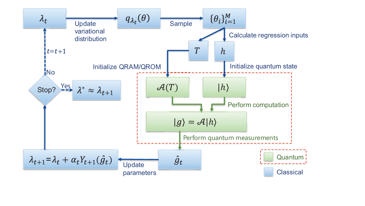
The quantum linear system algorithm provides an efficient way to estimate the natural gradient $g$, but its output is a quantum state $\ket{g}$. To use $\ket{g}$ in VB, we face a design choice: either use $\ket{g}$ in a quantum algorithm – i.e. run the entire VB gradient descent algorithm on a quantum computer – or read out the information encoded in $\ket{g}$ for use on a classical computer. Even though readout can be a resource-intensive step, we propose to use a hybrid quantum-classical approach, illustrated in Figure 1, where the quantum computer calculates $\ket{g}$, and the classical computer uses the information to update parameters $\lambda$, to sample from the variational distribution $q_{\lambda}(\theta)$, and to estimate the likelihood vector $h$ and the design matrix $T$.

The hybrid quantum-classical approach is more suitable for VB gradient descent because iterative quantum algorithms are, in general, resource intensive. Quantum transformations are linear; to create effectively non-linear transformations repeated quantum registers are used, some of which are destroyed using projective quantum measurements (Gilyén et al. 2019; Rebentrost et al. 2019, see, e.g.). If the projective measurement yields the desired result with probability $p<1$ (usually $p\leq 1/2)$, the measurement destroys, on average, $1/p-1$ quantum registers. For an iterative quantum algorithm to yield the desired result after $T$ iterations, $O(p^{-T})$ qubit registers are required. Therefore, end-to-end quantum algorithms work for iterative computations only if a few iterative steps are sufficient. Bausch Bausch 2020 proposes a recurrent method with post-selection in the context of quantum Recurrent Neural Networks and argues that, for approximate post-selection it is possible to reduce this overhead. Another possible approach is to run the iterative algorithm without post-selection for $T$ steps and then amplify the desired end state using Quantum Amplitude Amplification (QAA) (Brassard et al. 2002). Even with these improvements, the exponential dependence on the number of iterations $T/z$ (where $z=2$ for QAA method) remains. For example, Rebentrost et al. Rebentrost et al. 2019 propose an end-to-end quantum algorithm to find the minimum of a homogeneous polynomial using Newton’s method (which leverages the density matrix exponentiation method of Lloyd et al. Lloyd et al. 2014), suitable for situations where only a few iterative steps are required. If an optimization requires more than a few iterative steps, a hybrid quantum-classical algorithm, such as the one proposed in this paper, is a better choice, provided it can handle the classical-quantum-classical handoff efficiently.

The hybrid quantum-classical VB algorithm with quantum natural descent is summarized in Algorithm 2. It extends the classical Algorithm 1 to embed a quantum subroutine to estimate the natural gradient. We consider two versions of the quantum natural gradient estimator: The first, Algorithm 3, includes full readout of the output state $\ket{g}$. The second, Algorithm 4, includes partial readout of $\ket{g}$ focused on the most significant coordinates of $g$. We describe the subroutines in the next two subsections.

The quantum natural gradient subroutine with full readout (Algorithm 3) starts with the initialization of the quantum state $\ket{h}$ and making available the entries of the design matrix $T$. Note that because $h$ is a vector of length $M$ and $M\ll N$, preparation of the input state $\ket{h}$ requires only $O(M/\log M)$ operations, negligible relative to the complexity of other parts of the algorithm. As discussed above, the computation of the $M\times N$ entries of matrix $T$ bounds from below the time complexity of both classical and quantum algorithms for natural gradient estimation. Once matrix $T$ is stored on a classical computer, time-efficient methods have been proposed to make it available for quantum computation either in a quantum random access memory (QRAM) Giovannetti et al. 2008a; Giovannetti et al. 2008b; Hann et al. 2021 or a classical read-only memory for quantum access (QROM) Kerenidis and Prakash 2016. With these inputs, the quantum computer executes a quantum linear systems algorithm (e.g. HHL or WPZ) to perform singular value inversion and the computation of the quantum state $\ket{g}$. The last step of the quantum subroutine is the readout of state $\ket{g}$ using a series of quantum measurements.

Since quantum measurement of state $\ket{g}$ in the basis $\{\ket{i}\}_{i=1}^{N}$ yields the state $\ket{i}$ with probability $|g_{i}|^{2}/\|g\|^{2}$, repeated measurements allow us to estimate $|g_{i}|/\|g\|$ – the normalized absolute values of each gradient coordinate. To extract the sign of $g_{i}$, an additional step is required. At the beginning of the quantum computation, we pull in an additional auxiliary qubit and apply a Hadamard gate (Nielsen and Chuang 2002; Lopatnikova et al. 2021, see, e.g.) to create two computational branches. In the computational branch of the auxiliary qubit in state $\ket{0}$ we run the HHL or WPZ algorithm to create the state $\ket{g}$; in the $\ket{1}$-branch we create the uniform state $\ket{\gamma}\equiv\frac{1}{\sqrt{N}}\sum_{i=1}^{N}\ket{i}$. The resulting state is

which is equivalent to

where $\ket{\pm}\equiv\frac{1}{\sqrt{2}}(\ket{0}\pm\ket{1})$ represent Hadamard basis states Nielsen and Chuang 2002; Lopatnikova et al. 2021 of the auxiliary qubit. To streamline notation and without loss of generality, we assumed $\|g\|=1$ (we discuss the implications of measuring $g/\|g\|$ rather than $g$ at the end of this subsection).

Simultaneous measurements of the register holding the superposition of $\ket{g}$ and $\ket{\gamma}$, which we call the data register, and the auxiliary register yield results that comprise an unbiased estimator of ${g}_{i}$. We measure the data register in the computational basis and the auxiliary qubit in the Hadamard basis. The probability of measuring the $\ket{\pm}$ state in the auxiliary qubit and $\ket{i}$ in the data register is $|g_{i}\pm\frac{1}{\sqrt{N}}|^{2}/4$. We perform repeated measurements and count the outcomes. Let $n^{\pm}_{i}$ be the number of measurements of the data register that yield the state $\ket{i}$ when the measurement of the auxiliary qubit yields $\ket{\pm}$, and $n_{T}=\sum_{i=1}^{N}(n^{+}_{i}+n^{-}_{i})$ be the total number of measurements taken. Let $\mathbb{E}_{m}$ indicate expectation over measurement results. Then,

which implies that measurement results yield an unbiased estimator of $g_{i}$:

We denote by $\widehat{g}=(\widehat{g}_{1},...,\widehat{g}_{N})^{\top}$ the quantum natural gradient which is a classical vector.

Technically, this algorithm results in a unbiased estimator of the normalized natural gradient, i.e. $g/\|g\|$, because of the unit norm requirement of quantum states in quantum computation. This makes quantum natural gradient suit naturally to gradient clipping (Section II.1) - a method used in stochastic gradient descent that clips off the length of the gradient vector to help stabilize the optimization Goodfellow et al. 2016.

Full readout of $g/\|g\|$ requires $O(N/\epsilon^{2})$ quantum measurements to estimate the vector $g$ within precision $\epsilon$. Full readout, however, may not be required when estimation of top gradient coordinates (by absolute value) is sufficient for VB convergence. We propose a new method we call the quantum Gauss-Southwell rule developed specifically for quantum natural gradient estimation (Algorithm 4). The method extracts one of the highest-value directions of the natural gradient estimate vector $g$ within precision $\epsilon$ using $O(\sqrt{N}/\epsilon)$ measurements.

The quantum Gauss-Southwell rule is a quantum analogue of the Gauss-Southwell rule for efficient classical coordinate descent Nutini et al. 2015. At each step of coordinate descent, the classical Gauss-Southwell rule selects the top gradient coordinate (by absolute value). Classical Gauss-Southwell rule can deliver efficient linear convergence even for high-dimensional models; its primary shortcoming is its computational intensity relative to randomized coordinate descent, because it requires the computation of the full gradient vector. The quantum approach estimates the full gradient vector highly efficiently in quantum parallel, making quantum Gauss-Southwell rule efficient and able to handle natural gradient Gauss-Southwell descent, infeasible on a classical computer.

Let $\ket{g}$ be the output state of the quantum natural gradient estimation algorithm. We measure $\ket{g}$ in the computational basis. The measurement yields a computational basis state $\ket{i}$ with probability $|g_{i}|^{2}$. The quantum measurement naturally yields the index of one of the highest absolute-value gradient directions with high probability, analogously to the classical Gauss-Southwell coordinate descent which selects the highest absolute-value gradient direction for the parameter update. Having determined the index $i$ of a significant gradient coordinate, we use Quantum Amplitude Estimation Brassard et al. 2002 with target state $\ket{i}$ to extract the value of $g_{i}$ in $O(\sqrt{N}/\epsilon)$ operations. Applying Quantum Amplitude Estimation directly to the state $\ket{g}$ yields the absolute value $|g_{i}|$ rather than the signed value $g_{i}$. As in the case of full readout (Section III.1), in order to extract the sign of $g_{i}$, we append an auxiliary qubit in order to be able to estimate $\frac{1}{2}\big|\frac{g_{i}}{\|g\|}\pm\frac{1}{\sqrt{N}}\big|$ as described in Algorithm 4:

Formal proof of convergence of quantum VB with Gauss-Southwell rule is outside the scope of this work and is a topic of future research.

The hybrid quantum-classical VB algorithm provides a flexible framework that can leverage one of a number of quantum, classical, or even classical quantum-inspired Tang 2018 algorithms for natural gradient estimation. The key factors in determining which natural gradient estimation algorithm is to be used are the number of samples $M$ and the condition number $\kappa$ of the design matrix $T$. The desired precision $\epsilon$ is also a driver of computational complexity, but it is not the limiting variable in the the stochastic approximation to the natural gradient. We compare two quantum algorithms – HHL and WPZ, with two measurement schemes (full readout and Gauss-Southwell rule) to read off $\hat{g}$ – with a classical singular value decomposition (SVD) algorithm and a quantum-inspired algorithm Gilyén et al. 2018.

Table 1 summarizes the time complexity of algorithms for natural gradient estimation. The time complexity of quantum algorithms takes into account quantum state preparation and readout. Each of the algorithms we consider is the most efficient algorithm in some regime defined by the scaling of $M$ and $\kappa$ with the size of the model $N$. Quantum algorithms are most efficient when $M=\tilde{O}(N^{\alpha})$, where $0<\alpha<1$, and $\kappa<C_{\kappa}M$, where $C_{\kappa}$ is a constant. When $\alpha=0$ and $\kappa=\tilde{O}(\text{poly}\,\log(N))$, i.e. the matrix $T$ is sparse and well-conditioned, quantum-inspired algorithms are most efficient. Table 2 summarizes the most efficient algorithms given $M$ and $\kappa$. The summary assumes that the scaling of all algorithms with problem size is bounded from below by the need to estimate the design matrix $T$; should more efficient ways to estimate non-zero entries of $T$ become available, quantum algorithms will become the most efficient choice across most combinations of $M$ and $\kappa$.

References

- Hoffman et al. (2013) M. D. Hoffman, D. M. Blei, C. Wang, and J. Paisley, Stochastic variational inference, Journal of Machine Learning Research 14, 1303 (2013).
- Kingma and Welling (2014) D. Kingma and M. Welling, Auto-encoding Variational Bayes, in 2nd International Conference on Learning Representations (2014).
- Zhang et al. (2018) C. Zhang, J. Bütepage, H. Kjellström, and S. Mandt, Advances in variational inference, IEEE transactions on pattern analysis and machine intelligence 41, 2008 (2018).
- Amari (1998) S.-I. Amari, Natural gradient works efficiently in learning, Neural Computation 10, 251 (1998).
- Sato (2001) M. Sato, Online model selection based on the variational Bayes, Neural Computation 13, 1649 (2001).
- Tran et al. (2017) M. Tran, D. Nott, and R. Kohn, Variational Bayes with intractable likelihood, Journal of Computational and Graphical Statistics 26, 873 (2017).
- Mishkin et al. (2018) A. Mishkin, F. Kunstner, D. Nielsen, M. Schmidt, and M. E. Khan, Slang: Fast structured covariance approximations for Bayesian deep learning with natural gradient, Neural Information Processing Systems (NIPS) (2018).
- Martens (2020) J. Martens, New insights and perspectives on the natural gradient method, Journal of Machine Learning Research 21, 1 (2020).
- Martens and Grosse (2015) J. Martens and R. Grosse, Optimizing neural networks with Kronecker-factored approximate curvature, in Proceedings of the 32nd International Conference on Machine Learning (2015) pp. 2408–2417.
- Tran et al. (2020) M.-N. Tran, N. Nguyen, D. Nott, and R. Kohn, Bayesian deep net glm and glmm, Journal of Computational and Graphical Statistics 29, 97 (2020).
- Harrow et al. (2009) A. W. Harrow, A. Hassidim, and S. Lloyd, Quantum algorithm for linear systems of equations, Physical Review Letters 103, 150502 (2009).
- Ambainis (2012) A. Ambainis, Variable time amplitude amplification and quantum algorithms for linear algebra problems, in STACS’12 (29th Symposium on Theoretical Aspects of Computer Science), Vol. 14 (LIPIcs, 2012) pp. 636–647.
- Clader et al. (2013) B. D. Clader, B. C. Jacobs, and C. R. Sprouse, Preconditioned quantum linear system algorithm, Physical Review Letters 110, 250504 (2013).
- Kerenidis and Prakash (2016) I. Kerenidis and A. Prakash, Quantum recommendation systems, arXiv preprint arXiv:1603.08675 (2016).
- Wossnig et al. (2018) L. Wossnig, Z. Zhao, and A. Prakash, Quantum linear system algorithm for dense matrices, Physical Review Letters 120, 050502 (2018).
- Childs et al. (2017) A. M. Childs, R. Kothari, and R. D. Somma, Quantum algorithm for systems of linear equations with exponentially improved dependence on precision, SIAM Journal on Computing 46, 1920 (2017).
- Subaşı et al. (2019) Y. Subaşı, R. D. Somma, and D. Orsucci, Quantum algorithms for systems of linear equations inspired by adiabatic quantum computing, Physical Review Letters 122, 060504 (2019).
- Gilyén et al. (2019) A. Gilyén, Y. Su, G. H. Low, and N. Wiebe, Quantum singular value transformation and beyond: exponential improvements for quantum matrix arithmetics, in Proceedings of the 51st Annual ACM SIGACT Symposium on Theory of Computing (2019) pp. 193–204.
- Aaronson (2015) S. Aaronson, Read the fine print, Nature Physics 11, 291 (2015).
- Tran et al. (2021a) M.-N. Tran, D. H. Nguyen, and D. Nguyen, Variational Bayes on manifolds, Statistics and Computing 31 (2021a).
- Tran et al. (2021b) M.-N. Tran, T.-N. Nguyen, and V.-H. Dao, A practical tutorial on variational bayes, arXiv:2103.01327 (2021b).
- Goodfellow et al. (2016) I. Goodfellow, Y. Bengio, and A. Courville, Deep Learning (MIT Press, 2016) http://www.deeplearningbook.org.
- Kobak et al. (2020) D. Kobak, J. Lomond, and B. Sanchez, The optimal ridge penalty for real-world high-dimensional data can be zero or negative due to the implicit ridge regularization, Journal of Machine Learning Research 21, 1 (2020).
- Liang et al. (2019) T. Liang, T. Poggio, A. Rakhlin, and J. Stokes, Fisher-rao metric, geometry, and complexity of neural networks, in The 22nd International Conference on Artificial Intelligence and Statistics (PMLR, 2019) pp. 888–896.
- Bartlett et al. (2020) P. L. Bartlett, P. M. Long, G. Lugosi, and A. Tsigler, Benign overfitting in linear regression, Proceedings of the National Academy of Sciences 117, 30063 (2020).
- Dar et al. (2021) Y. Dar, V. Muthukumar, and R. G. Baraniuk, A farewell to the bias-variance tradeoff? an overview of the theory of overparameterized machine learning, arXiv preprint arXiv:2109.02355 (2021).
- Salimans et al. (2013) T. Salimans, D. A. Knowles, et al., Fixed-form variational posterior approximation through stochastic linear regression, Bayesian Analysis 8, 837 (2013).
- Malago et al. (2013) L. Malago, M. Matteucci, and G. Pistone, Natural gradient, fitness modelling and model selection: A unifying perspective, in 2013 IEEE Congress on Evolutionary Computation (IEEE, 2013) pp. 486–493.
- (29) Note that the conjugate gradient method Shewchuk et al. 1994; Saad 2003, sometimes used as a classical benchmark for quantum linear systems algorithms Clader et al. 2013, does not apply to the natural gradient problem. The conjugate gradient method requires that the inverted matrix is symmetric and positive definite. The design matrix is not symmetric and its symmetrized version is not positive definite.
- Wiebe et al. (2014) N. Wiebe, A. Kapoor, and K. M. Svore, Quantum deep learning, arXiv preprint arXiv:1412.3489 (2014).
- Schuld et al. (2016) M. Schuld, I. Sinayskiy, and F. Petruccione, Prediction by linear regression on a quantum computer, Physical Review A 94, 022342 (2016).
- Wang (2017) G. Wang, Quantum algorithm for linear regression, Physical Review A 96, 012335 (2017).
- Liu et al. (2019) H.-L. Liu, C.-H. Yu, Y.-S. Wu, S.-J. Pan, S.-J. Qin, F. Gao, and Q.-Y. Wen, Quantum algorithm for logistic regression, arXiv preprint arXiv:1906.03834 (2019).
- Yu et al. (2021) C.-H. Yu, F. Gao, and Q. Wen, An improved quantum algorithm for ridge regression, IEEE Transactions on Knowledge and Data Engineering 33, 858 (2021).
- Potok et al. (2021) T. Potok et al., Adiabatic quantum linear regression, Scientific Reports 11, 1 (2021).
- Schuld and Petruccione (2018) M. Schuld and F. Petruccione, Supervised learning with quantum computers (Springer, 2018).
- Lopatnikova et al. (2021) A. Lopatnikova, M.-N. Tran, and S. A. Sisson, An introduction to quantum computing for statisticians and data scientists, arXiv preprint arXiv:2112.06587 (2021).
- Berry et al. (2015) D. W. Berry, A. M. Childs, and R. Kothari, Hamiltonian simulation with nearly optimal dependence on all parameters, in 2015 IEEE 56th Annual Symposium on Foundations of Computer Science (IEEE, 2015) pp. 792–809.
- Aharonov and Ta-Shma (2003) D. Aharonov and A. Ta-Shma, Adiabatic quantum state generation and statistical zero knowledge, in Proceedings of the 35th Annual ACM Symposium on Theory of Computing (2003) pp. 20–29.
- Gilyén et al. (2018) A. Gilyén, S. Lloyd, and E. Tang, Quantum-inspired low-rank stochastic regression with logarithmic dependence on the dimension, arXiv preprint arXiv:1811.04909 (2018).
- Frieze et al. (2004) A. Frieze, R. Kannan, and S. Vempala, Fast monte-carlo algorithms for finding low-rank approximations, Journal of the ACM (JACM) 51, 1025 (2004).
- Rebentrost et al. (2019) P. Rebentrost, M. Schuld, L. Wossnig, F. Petruccione, and S. Lloyd, Quantum gradient descent and Newton’s method for constrained polynomial optimization, New Journal of Physics 21, 073023 (2019).
- (43) Bausch Bausch 2020 proposes a recurrent method with post-selection in the context of quantum Recurrent Neural Networks and argues that, for approximate post-selection it is possible to reduce this overhead. Another possible approach is to run the iterative algorithm without post-selection for steps and then amplify the desired end state using Quantum Amplitude Amplification (QAA) (Brassard et al. 2002). Even with these improvements, the exponential dependence on the number of iterations (where for QAA method) remains.
- (44) The algorithm leverages the density matrix exponentiation method of Lloyd et al. Lloyd et al. 2014.
- Giovannetti et al. (2008a) V. Giovannetti, S. Lloyd, and L. Maccone, Quantum random access memory, Physical Review Letters 100, 160501 (2008a).
- Giovannetti et al. (2008b) V. Giovannetti, S. Lloyd, and L. Maccone, Architectures for a quantum random access memory, Physical Review A 78, 052310 (2008b).
- Hann et al. (2021) C. T. Hann, G. Lee, S. Girvin, and L. Jiang, Resilience of quantum random access memory to generic noise, PRX Quantum 2, 020311 (2021).
- Nielsen and Chuang (2002) M. A. Nielsen and I. Chuang, Quantum computation and quantum information (2002).
- Nutini et al. (2015) J. Nutini, M. Schmidt, I. Laradji, M. Friedlander, and H. Koepke, Coordinate descent converges faster with the gauss-southwell rule than random selection, in International Conference on Machine Learning (PMLR, 2015) pp. 1632–1641.
- Brassard et al. (2002) G. Brassard, P. Hoyer, M. Mosca, and A. Tapp, Quantum amplitude amplification and estimation, Contemporary Mathematics 305, 53 (2002).
- Tang (2018) E. Tang, Quantum-inspired classical algorithms for principal component analysis and supervised clustering, arXiv preprint arXiv:1811.00414 (2018).
- Papamakarios et al. (2021) G. Papamakarios, E. Nalisnick, D. Rezende, S. Mohamed, and B. Lakshminarayanan, Normalizing flows for probabilistic modeling and inference, Journal of Machine Learning Research 22, 1 (2021).
- Wiebe et al. (2012) N. Wiebe, D. Braun, and S. Lloyd, Quantum algorithm for data fitting, Physical Review Letters 109, 050505 (2012).
- Duan et al. (2017) B. Duan, J. Yuan, Y. Liu, and D. Li, Quantum algorithm for support matrix machines, Physical Review A 96, 032301 (2017).
- Wang et al. (2019) D. Wang, O. Higgott, and S. Brierley, Accelerated variational quantum eigensolver, Physical Review Letters 122, 140504 (2019).
- Kerenidis and Prakash (2020) I. Kerenidis and A. Prakash, Quantum gradient descent for linear systems and least squares, Physical Review A 101, 022316 (2020).
- Low et al. (2014) G. H. Low, T. J. Yoder, and I. L. Chuang, Quantum inference on Bayesian networks, Physical Review A 89, 062315 (2014).
- Rebentrost et al. (2014) P. Rebentrost, M. Mohseni, and S. Lloyd, Quantum support vector machine for big data classification, Physical Review Letters 113, 130503 (2014).
- McClean et al. (2016) J. R. McClean, J. Romero, R. Babbush, and A. Aspuru-Guzik, The theory of variational hybrid quantum-classical algorithms, New Journal of Physics 18, 023023 (2016).
- Rebentrost et al. (2018) P. Rebentrost, T. R. Bromley, C. Weedbrook, and S. Lloyd, Quantum Hopfield neural network, Physical Review A 98, 042308 (2018).
- Harrow and Napp (2019) A. Harrow and J. Napp, Low-depth gradient measurements can improve convergence in variational hybrid quantum-classical algorithms, arXiv preprint arXiv:1901.05374 (2019).
- McArdle et al. (2019) S. McArdle, T. Jones, S. Endo, Y. Li, S. C. Benjamin, and X. Yuan, Variational ansatz-based quantum simulation of imaginary time evolution, npj Quantum Information 5, 1 (2019).
- Schuld and Killoran (2019) M. Schuld and N. Killoran, Quantum machine learning in feature Hilbert spaces, Physical Review Letters 122, 040504 (2019).
- Schuld et al. (2020) M. Schuld, A. Bocharov, K. M. Svore, and N. Wiebe, Circuit-centric quantum classifiers, Physical Review A 101, 032308 (2020).
- Abbas et al. (2020) A. Abbas, D. Sutter, C. Zoufal, A. Lucchi, A. Figalli, and S. Woerner, The power of quantum neural networks, arXiv preprint arXiv:2011.00027 (2020).
- Park and Kastoryano (2020) C.-Y. Park and M. J. Kastoryano, Geometry of learning neural quantum states, Physical Review Research 2, 023232 (2020).
- Miyahara and Sughiyama (2018) H. Miyahara and Y. Sughiyama, Quantum extension of variational Bayes inference, Physical Review A 98, 022330 (2018).
- Zhao et al. (2019) Z. Zhao, A. Pozas-Kerstjens, P. Rebentrost, and P. Wittek, Bayesian deep learning on a quantum computer, Quantum Machine Intelligence 1, 41 (2019).
- Jordan (2005) S. P. Jordan, Fast quantum algorithm for numerical gradient estimation, Physical Review Letters 95, 050501 (2005).
- Schuld et al. (2019) M. Schuld, V. Bergholm, C. Gogolin, J. Izaac, and N. Killoran, Evaluating analytic gradients on quantum hardware, Physical Review A 99, 032331 (2019).
- Stokes et al. (2020) J. Stokes, J. Izaac, N. Killoran, and G. Carleo, Quantum natural gradient, Quantum 4, 269 (2020).
- Sweke et al. (2020) R. Sweke, F. Wilde, J. J. Meyer, M. Schuld, P. K. Fährmann, B. Meynard-Piganeau, and J. Eisert, Stochastic gradient descent for hybrid quantum-classical optimization, Quantum 4, 314 (2020).
- Gacon et al. (2021) J. Gacon, C. Zoufal, G. Carleo, and S. Woerner, Simultaneous perturbation stochastic approximation of the quantum fisher information, arXiv preprint arXiv:2103.09232 (2021).
- Mitarai et al. (2018) K. Mitarai, M. Negoro, M. Kitagawa, and K. Fujii, Quantum circuit learning, Physical Review A 98, 032309 (2018).
- Zoufal et al. (2019) C. Zoufal, A. Lucchi, and S. Woerner, Quantum generative adversarial networks for learning and loading random distributions, npj Quantum Information 5, 1 (2019).
- Zoufal et al. (2020) C. Zoufal, A. Lucchi, and S. Woerner, Variational quantum Boltzmann machines, arXiv preprint arXiv:2006.06004 (2020).
- (77) Consider a discretization with points for each dimension. It would require an dimensional Hilbert space and qubits.
- Reiher et al. (2017) M. Reiher, N. Wiebe, K. M. Svore, D. Wecker, and M. Troyer, Elucidating reaction mechanisms on quantum computers, Proceedings of the National Academy of Sciences 114, 7555 (2017).
- Aspuru-Guzik et al. (2018) A. Aspuru-Guzik, R. Lindh, and M. Reiher, The matter simulation (r) evolution, ACS Central Science 4, 144 (2018).
- Cao et al. (2018) Y. Cao, J. Romero, and A. Aspuru-Guzik, Potential of quantum computing for drug discovery, IBM Journal of Research and Development 62, 6 (2018).
- McArdle et al. (2020) S. McArdle, S. Endo, A. Aspuru-Guzik, S. C. Benjamin, and X. Yuan, Quantum computational chemistry, Reviews of Modern Physics 92, 015003 (2020).
- Babbush et al. (2018) R. Babbush, N. Wiebe, J. McClean, J. McClain, H. Neven, and G. K.-L. Chan, Low-depth quantum simulation of materials, Physical Review X 8, 011044 (2018).
- Macridin et al. (2018) A. Macridin, P. Spentzouris, J. Amundson, and R. Harnik, Electron-phonon systems on a universal quantum computer, Physical Review Letters 121, 110504 (2018).
- Ajagekar and You (2019) A. Ajagekar and F. You, Quantum computing for energy systems optimization: Challenges and opportunities, Energy 179, 76 (2019).
- Robert et al. (2021) A. Robert, P. K. Barkoutsos, S. Woerner, and I. Tavernelli, Resource-efficient quantum algorithm for protein folding, npj Quantum Information 7, 1 (2021).
- Stamatopoulos et al. (2020) N. Stamatopoulos, D. J. Egger, Y. Sun, C. Zoufal, R. Iten, N. Shen, and S. Woerner, Option pricing using quantum computers, Quantum 4, 291 (2020).
- Shewchuk et al. (1994) J. R. Shewchuk et al., An introduction to the conjugate gradient method without the agonizing pain (1994).
- Saad (2003) Y. Saad, Iterative methods for sparse linear systems (SIAM, 2003).
- Bausch (2020) J. Bausch, Recurrent quantum neural networks, Advances in Neural Information Processing Systems 33 (2020).
- Lloyd et al. (2014) S. Lloyd, M. Mohseni, and P. Rebentrost, Quantum principal component analysis, Nature Physics 10, 631 (2014).