Outlier-Robust Filtering For Nonlinear Systems With Selective Observations Rejection

We resort to the unscented Kalman filter (UKF) as the basic inferential engine, approximating the Gaussian integrals using the unscented transform [11], for all the considered methods. Therefore, we name the proposed method as selective observations-rejecting UKF (SOR-UKF). Similarly, the other VB-based outlier-robust baseline filters are called as recursive outlier-robust UKF (ROR-UKF) [23], switching error model UKF (SEM-UKF) [20] and outlier-detecting UKF (OD-UKF) [28]. The choice of using UKF allows us to propose a computationally efficient modification of our devised filter based on an available efficient implementation of UKF for handling high-dimensional uncorrelated measurements reported in literature [38].

Since the baseline methods, in their original form, do not treat the outliers selectively for each dimension (as these are under-parameterized in terms of outlier detection for each dimension), we modify each of these for such behavior. In particular, the measurements from each sensor at each time step are proposed to be used in turn i.e. the final estimate using any sensor’s observation serves as the prediction for the update using the next sensor’s measurement. Accordingly, the modified baseline algorithms are referred to as mROR-UKF, mSEM-UKF, and mOD-UKF.

Moreover, we propose using an alternate implementation of the proposed SOR-UKF, referred to as mSOR-UKF with lower complexity. Since $\mathbf{V}^{-1}_{k}$ is diagonal, the basic inferential UKF used within the proposed SOR-UKF can be modified from the standard parallel sigma point Kalman filter (P-SPKF) to the serial sigma point Kalman filter (S-SPKF) [38] for use in mSOR-UKF. Note that S-SPKF can be also used in conjunction with ROR-UKF, SEM-UKF and OD-UKF, as originally reported, but these do not treat outliers selectively for each dimension hence compromising the estimation quality. mROR-UKF, mSEM-UKF and mOD-UKF, on the other hand, have analogous structures to the serial re-draw sigma point Kalman filter (SRD-SPKF) in [38].

In all the simulations and experimental scenarios, we use Matlab on an Intel i7-8550U processor powered computer and consider SI units. First, we choose to simulate a target tracking application for performance evaluation.

Fig. 1 shows the testing setup for a target tracking example we consider in the simulations for performance evaluation. Maneuvering targets with unknown turn rates are commonly modeled as

where the state vector $\mathbf{x}_{k}=[a_{k},\dot{{a_{k}}},b_{k},\dot{{b_{k}}},\omega_{k}]^{\text{T}}$ contains the 2D position coordinates $({a_{k}},{b_{k}})$, the corresponding velocities $(\dot{{a_{k}}},\dot{{b_{k}}})$, the angular velocity $\omega_{k}$ of the target at time instant $k$, $\Delta t$ is the sampling period, and $\mathbf{q}_{k-\text{1}}\sim N\left(0,\mathbf{Q}_{k-\text{1}}.\right)$ with $\mathbf{Q}_{k-\text{1}}$ given, in terms of scaling parameters $\eta_{1}$ and $\eta_{2}$, as [28]

We consider that angle and range readings are obtained from sensors, installed around a rectangular area, at $m$ different locations. A total of $m/2$ independent sensors are used to provide angle readings where its $j$th sensor is present at the 2D coordinate $(a^{\theta_{j}}=350(j-1),b^{\theta_{j}}=350(j\mod 2))$. Similarly, range measurements are obtained from the other $m/2$ independent sensors where its $j$th sensor is located at $(a^{\rho_{j}}=350(j-1),b^{\rho_{j}}=350\ ((j-1)\mod 2))$.

For performance evaluation, two subcases of how measurements from different sensors get disturbed are considered. First, we suppose outliers explicitly add in the observations randomly. Subsequently, we evaluate the case of missing data.

We suppose a Gaussian mixture to model the additive effect of outliers commonly used for performance evaluation of robust filtering methods[20, 28]. The measurement vector $\mathbf{y}_{k}$ considering the additive effect of independently occurring outliers in different dimensions can be expressed as

where $\mathbf{s}_{k}=[s^{\theta_{1}}_{k}...s^{\theta_{{m}/{2}}}_{k},s^{\rho_{1}}_{k}...s^{\rho_{m/2}}_{k}]^{\text{T}}$ and $\mathbf{o}_{k}=[o^{\theta_{1}}_{k}...o^{\theta_{m/2}}_{k},o^{\rho_{1}}_{k}...o^{\rho_{m/2}}_{k}]^{\text{T}}$ denote the noise-free and noisy components of $\mathbf{y}_{k}$ respectively. The entries of $\mathbf{s}_{k}$, $s^{\theta_{j}}_{k}$ and $s^{\rho_{j}}_{k}$, which denote the noise-free values corresponding to $j$th bearing and range sensors respectively are given as

Similarly, the entries of $\mathbf{o}_{k}$, $o^{\theta_{j}}_{k}$ and $o^{\rho_{j}}_{k}$, control the noise content in the measurements from the $j$th bearing and range sensors. $\mathbf{o}_{k}$ is considered to obey the following distribution

where ${\sigma_{\theta}}^{2}$ and ${\sigma_{\rho}}^{2}$ are the variances of nominal noise in angle and range readings respectively. The parameters $\lambda$ and $\gamma$ control the frequency and variance of an outlier in each dimension respectively.

The following values of parameters are used (unless stated otherwise): the initial state $\mathbf{x}_{0}=[-10000,10,5000,-5,-0.0524]^{\text{T}}$, $\triangle t=1$, $\eta_{1}=0.1$, $\eta_{2}=1.75\times 10^{-4}$, ${\sigma_{\theta}}=3.5\times 10^{-3}$, ${\sigma_{\rho}}=10$ and $m=6$. The initialization parameters of filters are: ${\mathbf{m}}^{+}_{0}\sim\mathcal{N}(\mathbf{x}_{0},\mathbf{P}^{+}_{0}$), $\mathbf{P}^{+}_{0}=100\mathbf{Q}_{k}$, $\epsilon=10^{-6}$ and $\theta^{i}_{k}=0.5~\forall~i$. For each method, the UKF parameters [11] are set as $\alpha=1$, $\beta=2$ and $\kappa=0$. Moreover, we use the same convergence threshold $\tau=10^{-4}$ and convergence metric $\delta$ for all the evaluated methods. Other parameters for the rival methods are assigned values as originally reported. All the simulations are repeated with a total time duration $K=1000$ and $100$ independent Monte Carlo (MC) runs.

First, we assess the tracking performance over time of different filters. Fig. 2 shows the Root Mean Squared Error of the position estimates $\text{RMSE}_{\text{pos}}$ over time for this scenario assuming $\lambda=0.3,\gamma\sim\mathcal{U}(100,1000)$. The methods which treat outliers selectively for each dimension i.e. SOR-UKF, mSOR-UKF, mROR-UKF, mSEM-UKF, and mOD-UKF exhibit comparable tracking performance whereas the other filters result in larger errors.

We also assess the quality of estimates using different filters with a change in $\lambda$ with $\gamma\sim\mathcal{U}(100,1000)$. Fig. 3 shows the box plots of the Root Mean Squared Error of the position estimates $\text{RMSE}_{\text{pos}}$ for this scenario. The methods dealing selectively with outliers exhibit comparable performance whereas the other filters result in a sharper rise of $\text{RMSE}_{\text{pos}}$ with an increase in $\lambda$.

Subsequently, we vary $\gamma$ and observe $\text{RMSE}_{\text{pos}}$ with $\lambda\sim\mathcal{U}(0,0.7)$. Fig. 4 shows the distributions of the $\text{RMSE}_{\text{pos}}$ for this case using different filters. SOR-UKF, mSOR-UKF, mROR-UKF, mSEM-UKF, and mOD-UKF demonstrate comparable performance and outperform other methods.

In addition, we evaluate how the change in nominal noise parameters ${\sigma_{\theta}}$ and ${\sigma_{\rho}}$ affects the performance of filters. Varying $\lambda$ the change in $\text{RMSE}_{\text{pos}}$ with $\gamma\sim\mathcal{U}(100,1000)$, ${\sigma_{\theta}}\sim\mathcal{U}(1.7\times 10^{-3},3.5\times 10^{-2})$, ${\sigma_{\rho}}\sim\mathcal{U}(5,50)$ is depicted in the box plots in Fig. 5. We observe a similar trend as in Fig. 3 except that the error magnitude levels increase.

In addition, we evaluate the robustness of SOR-UKF and mSOR-UKF with change in filter parameters by assuming $\epsilon\sim\mathcal{U}(10^{-7},10^{-3})$ and $\theta^{i}_{k}\sim\mathcal{U}(0.05,0.95)$ with $\gamma\sim\mathcal{U}(100,1000)$. Varying $\lambda$ the change in $\text{RMSE}_{\text{pos}}$ is depicted in the box plots in Fig. 6. We find the proposed filters quite robust to changes in filter parameters except at large values of $\lambda$ where the SOR-UKF and mSOR-UKF exhibit larger errors.

We also simulate a case where the effect of increase in the number of sensors on the estimation quality is observed. Fig. 7 depicts the $\text{RMSE}_{\text{pos}}$ versus $m$, increased from 200 to 1000, for methods dealing each dimension selectively. We choose a high rate of outlier occurrence i.e. $\lambda=0.9$ with $\gamma\sim\mathcal{U}(100,1000)$. Owing to a large dimensionality of $m$, or more sources of information, we see that most of the algorithms result in low errors especially at higher values of $m$. We find SOR-UKF and mSOR-UKF comparatively more robust in this scenario. Note that non-selective methods exhibit higher errors so we skip them in the results.

Lastly, we compare the computational cost for the selective methods exhibiting comparable lower $\text{RMSE}_{\text{pos}}$ values. We evaluate these methods in terms of the time taken to complete the Monte Carlo simulations. Setting $\lambda=0.9$ with $\gamma\sim\mathcal{U}(100,1000)$, we vary $m$ and present the distributions of completion times of simulations using different filters in Fig. 8. With increasing $m$, the average completion times of the simulations increase for all the filters. We observe that the empirical computational overhead verifies the theoretical complexity. SOR-UKF exhibits cubic complexity whereas the other techniques have linear complexity in terms of $m$. The differences in the processing overhead among mROR-UKF, mSEM-UKF, and mOD-UKF depends on the their modeling parameters and inferential mechanism. Importantly, we note that with an increase in $m$, the computational costs of mROR-UKF, mSEM-UKF, and mOD-UKF rise more steeply than the mSOR-UKF as predicted by the theoretical complexity (analogous to how S-SPKF is computationally faster than the SRD-SPKF) in [38]).

We also evaluate the performance of different filters for the case of missing data. Missing observations can also be viewed as special case of outliers in a sense that the nominal model in (1)-(2) is unable to describe the observations and only the modified measurement equation (6) can with ${{\mathcal{I}}}^{i}_{k}=\epsilon$ in any particular affected dimension $i$. Using the base parameters, as in the case of outliers, we simulate this case with $\lambda$ indicating the probability of missing observations in each dimension.

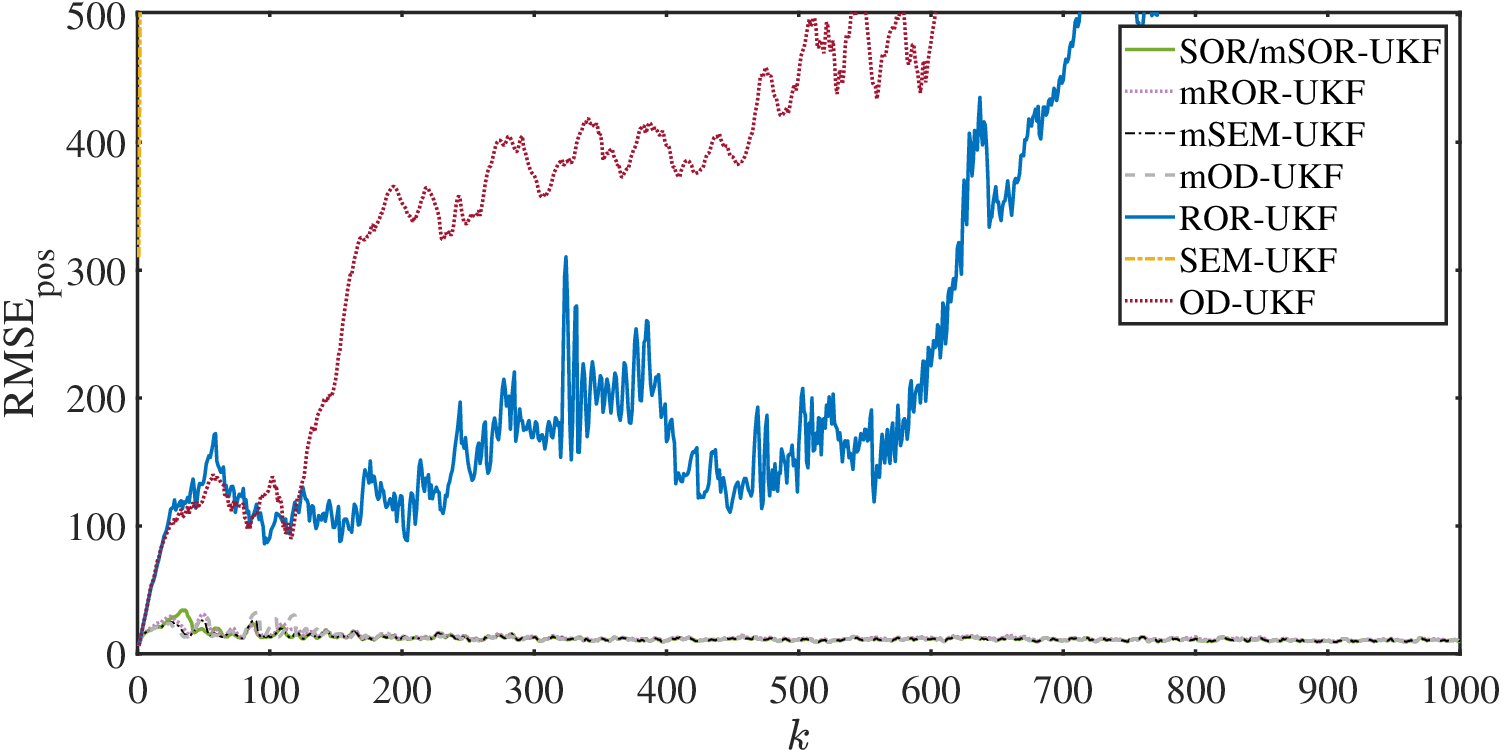
We observe similar results as for the case of outliers. Fig. 9 shows the tracking error of different algorithms over time with $\lambda=0.3$. We again find the selective methods exhibiting lower errors.

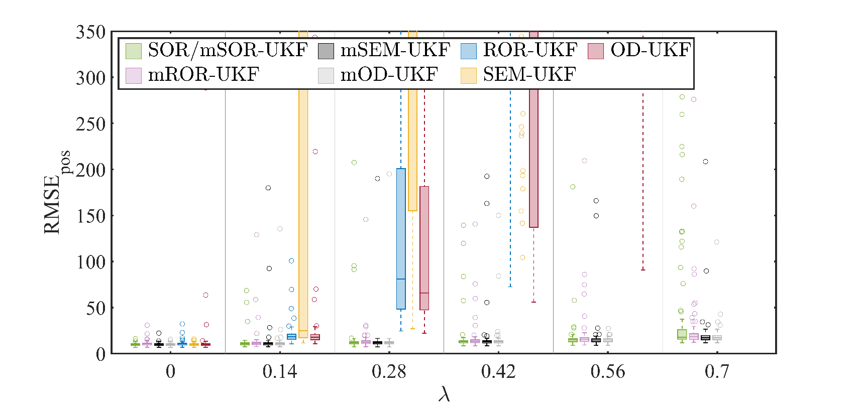
Fig. 10 shows the box plots of $\text{RMSE}_{\text{pos}}$ with change in $\lambda$ which reaffirms the superiority of methods dealing each dimension independently. However, we observe more degraded performances of non-selective methods compared to the case of outliers, drawn from a Gaussian mixture model, with increase in $\lambda$ especially the compensation-based methods i.e. SEM-UKF and ROR-UKF. These methods try to extract information from the measurement vector by learning the scaling parameters of their respective Gaussian covariance matrices given the abnormalities in data. This may be more suitable for certain applications and is not useful generally for unknown clutter or ”nonsense outliers” in words of the authors of SEM-UKF. For more detailed discussion where such non-selective compensating models are more useful the readers are referred to the Discussion Section of SEM-UKF pg. 8 [20].

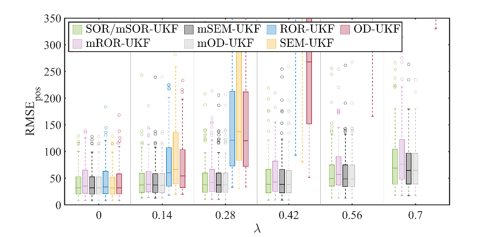
Fig. 11 shows the box plots of $\text{RMSE}_{\text{pos}}$ with change in $\lambda$ by assuming ${\sigma_{\theta}}\sim\mathcal{U}(1.7\times 10^{-3},3.5\times 10^{-2})$ and ${\sigma_{\rho}}\sim\mathcal{U}(5,50)$ to depict how the change in nominal noise statistics affect the estimation performance. The results have a similar trend as in Fig. 10 with a change that the error magnitude levels increase.

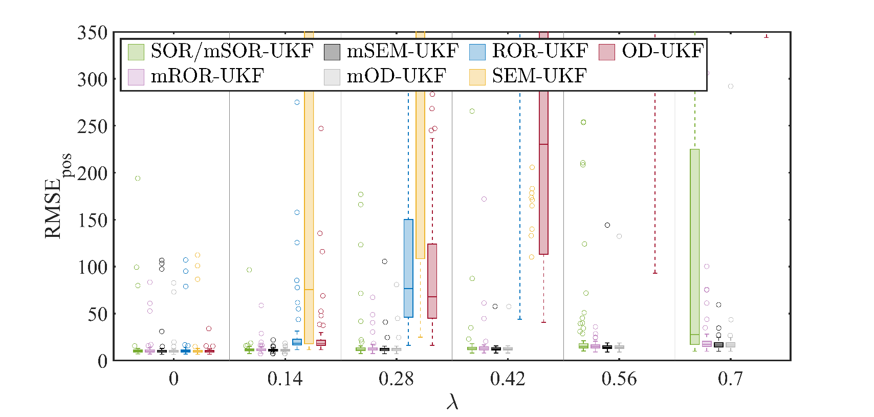
To test the robustness of the proposed filters with variations in filter parameters we assume $\epsilon\sim\mathcal{U}(10^{-7},10^{-3})$ and $\theta^{i}_{k}\sim\mathcal{U}(0.05,0.95)$. With variation in $\lambda$, box plots of $\text{RMSE}_{\text{pos}}$ are given in Fig. 12. Similar to the case of outliers, we observe the proposed algorithms to be quite robust to changes in filter parameters except at larger values of $\lambda$ where these produce more estimation errors.

As for the case of outliers in the previous case, we evaluate the comparative performance of methods dealing each dimension selectively with increase in $m$ and observe a similar trend for $\lambda=0.9$ as depicted in Fig. 13. in this case the estimation quality remains similar for each method.

For the computational complexity we have observed a similar trend for the case of missing observations as reported for the case of outliers as reported in Fig. 8.

Lastly, note that a case might arise where any actual measurement is close to zero e.g. the target may be very close to any range sensor in the simulation example. For this case, the nominal model would be able to explain the data as a result the measurement would be used for inference instead of being discarded. We have also simulated this case by initializing the target very close to a range sensor’s coordinates and repeating the missing observations simulations to test the robustness of the filters. For this case, we arrive at the similar results as reported above for the case of missing data simulations.

To test the comparative performance of the proposed method in practical settings, we carry out experimental campaigns at three sites for real-time indoor positioning using Ultra-wide band (UWB) devices. We use MDEK1001 Development Kit, by Qorvo, which includes 12 UWB units based on the DWM1001 module. The module’s on-board firmware drives the built-in UWB transceiver to form a network of anchor nodes and perform the two-way ranging exchanges with the tag nodes which enables each tag to compute its relative location to the anchors. For detailed information regarding the kit functionality readers can consult its freely available documentation. Figs. 16-16 show the experimental scenarios at three different locations including a corridor in the School of Science and Engineering (SSE) building, a corridor in the Academic Block (AB) and the entrance of the SSE building at the Lahore University of Management Sciences. For each of the experimental scenario, 1 unit is configured as a tag and rest of the 11 units are set in the anchor mode. In each scenario, all the 11 anchors are installed at predefined locations. Moreover, the tag traverses through a predetermined path whose step coordinates are known. The kit is used in its default configuration mode in which at a given time a maximum of 4 range readings are obtained from the closest anchors. The tag is attached to a laptop which logs the range data at each step traversed. The range data is obtained at 5Hz which is subsequently averaged to provide the final sensor readings at each step. The datasets generated from the experimental campaigns are available openly: https://github.com/chughtaiah/UWB_Data.

There are two major sources of outliers in the range data.

Firstly, there are missing observations in the data, since at most 4 out of 11 anchors provide data at a given time. The missing measurements are outliers in the data and contain no useful information. Secondly, UWB range data suffers from bias when the corresponding transceivers face physical obstruction during transmission known as the nonline-of-sight (NLoS) condition. Fig. 17 shows example of how the range data obtained from a UWB sensor node during the experimental campaign is corrupted by the two types of outliers.

We consider random walk as the state mobility dynamic model which has historically been used for inference in different applications including mobile nodes in wireless sensor networks [39]. Keeping the 2D position of the target as our quantity of interest, the state vector $\mathbf{x}_{k}=[a_{k},b_{k}]^{\text{T}}$ evolves with $\textbf{f}(.)=\mathbf{I}$ in (1). Moreover, the nominal measurement model, $\textbf{h}(.)$ in (2), has a functional form of range data as in (26) including the term for the $z$-axis for the locations of the tag and the anchors. In addition, $\mathbf{Q}_{k-\text{1}}$ and $\mathbf{R}_{k}$ are diagonal matrices with entries as 0.1. For each case, we set $\mathbf{x}_{0}=[0,0]^{\text{T}}$ and initialize the filters randomly with ${\mathbf{m}}^{+}_{0}\sim\mathcal{N}(\mathbf{x}_{0},\mathbf{P}^{+}_{0}$) where $\mathbf{P}^{+}_{0}=0.5\mathbf{I}$. We carry out 100 independent MC runs, keeping all other applicable parameters for the methods under consideration same as the base parameters.

We consider only the methods dealing outliers selectively with least computational complexity. Figs. 18-20 show the tracking performance of these filters. We observe that for cases 1 and 2 the methods exhibit similar tracking performances since the measurement mostly have missing observations as outliers for these cases. For case 3, the since data of some anchors is unusually contaminated with sporadic bias, in addition to the missing observations, the tracking error is larger in this case. In fact, tracking performance of mROR-UKF severely degrades for the third case due to unusual data corruption.

Table II summarizes the performance evaluation results of the considered algorithms in the experimental settings in terms of RMSE and average computational run time for each case. We notice that the achieved RMSE in each case, normally remaining in the sub-meter range, is comparative for each algorithm. There is an exception for Scenario 3 where mROR-UKF exhibits larger errors due to more NLoS conditions resulting in occurrence of more bias in data. The proposed mSOR-UKF leads in terms of RMSE error and more importantly has the least processing overhead indicating its practical usefulness in real-world scenarios.

References

- [1] E. Ghysels and M. Marcellino, Applied economic forecasting using time series methods. Oxford University Press, 2018.
- [2] A. C. Smith and E. N. Brown, “Estimating a state-space model from point process observations,” Neural Computation, vol. 15, no. 5, pp. 965–991, 2003.
- [3] R. Roesser, “A discrete state-space model for linear image processing,” IEEE Transactions on Automatic Control, vol. 20, no. 1, pp. 1–10, 1975.
- [4] D. Van Hertem, O. Gomis-Bellmunt, and J. Liang, State-space representation of HVDC grids, 2016, pp. 333–343.
- [5] L. Paninski, Y. Ahmadian, D. G. Ferreira, S. Koyama, K. R. Rad, M. Vidne, J. Vogelstein, and W. Wu, “A new look at state-space models for neural data,” Journal of computational neuroscience, vol. 29, no. 1-2, pp. 107–126, 2010.
- [6] P. Chauchat, J. Vilà-Valls, and E. Chaumette, “Robust information filtering under model mismatch for large-scale dynamic systems,” IEEE Control Systems Letters, pp. 1–1, 2021.
- [7] D.-J. Jwo and S.-H. Wang, “Adaptive fuzzy strong tracking extended Kalman filtering for GPS navigation,” IEEE Sensors Journal, vol. 7, no. 5, pp. 778–789, 2007.
- [8] A. Assa and F. Janabi-Sharifi, “A Kalman filter-based framework for enhanced sensor fusion,” IEEE Sensors Journal, vol. 15, no. 6, pp. 3281–3292, 2015.
- [9] R. E. Kalman, “A new approach to linear filtering and prediction problems,” 1960.
- [10] R. P. Wishner, J. A. Tabaczynski, and M. Athans, “A comparison of three non-linear filters,” Automatica, vol. 5, no. 4, pp. 487–496, 1969.
- [11] E. A. Wan, R. Van Der Merwe, and S. Haykin, “The unscented Kalman filter,” Kalman filtering and neural networks, vol. 5, no. 2007, pp. 221–280, 2001.
- [12] A. H. Chughtai, M. Tahir, and M. Uppal, “A robust Bayesian approach for online filtering in the presence of contaminated observations,” IEEE Transactions on Instrumentation and Measurement, pp. 1–1, 2020.
- [13] M. R. Fernandes, J. B. R. do Val, and R. F. Souto, “Robust estimation and filtering for poorly known models,” IEEE Control Systems Letters, vol. 4, no. 2, pp. 474–479, 2020.
- [14] S. Kim, V. M. Deshpande, and R. Bhattacharya, “Robust Kalman filtering with probabilistic uncertainty in system parameters,” IEEE Control Systems Letters, vol. 5, no. 1, pp. 295–300, 2021.
- [15] C. D. Karlgaard, “Nonlinear regression Huber–Kalman filtering and fixed-interval smoothing,” Journal of guidance, control, and dynamics, vol. 38, no. 2, pp. 322–330, 2015.
- [16] L. Chang and K. Li, “Unified form for the robust Gaussian information filtering based on M-estimate,” IEEE Signal Processing Letters, vol. 24, no. 4, pp. 412–416, 2017.
- [17] L. Chang, B. Hu, G. Chang, and A. Li, “Multiple outliers suppression derivative-free filter based on unscented transformation,” Journal of guidance, control, and dynamics, vol. 35, no. 6, pp. 1902–1906, 2012.
- [18] Y. Huang, Y. Zhang, N. Li, and J. Chambers, “Robust Student’s t based nonlinear filter and smoother,” IEEE Transactions on Aerospace and Electronic Systems, vol. 52, no. 5, pp. 2586–2596, 2016.
- [19] H. Wang, H. Li, W. Zhang, and H. Wang, “Laplace ℓ1 robust Kalman filter based on majorization minimization,” in 2017 20th International Conference on Information Fusion (Fusion), 2017, pp. 1–5.
- [20] A. Nakabayashi and G. Ueno, “Nonlinear filtering method using a switching error model for outlier-contaminated observations,” IEEE Transactions on Automatic Control, vol. 65, no. 7, pp. 3150–3156, 2020.
- [21] D. Xu, C. Shen, and F. Shen, “A robust particle filtering algorithm with non-Gaussian measurement noise using Student-t distribution,” IEEE Signal Processing Letters, vol. 21, no. 1, pp. 30–34, 2014.
- [22] H. Du, W. Wang, and L. Bai, “Observation noise modeling based particle filter: An efficient algorithm for target tracking in glint noise environment,” Neurocomputing, vol. 158, pp. 155–166, 2015.
- [23] R. Piché, S. Särkkä, and J. Hartikainen, “Recursive outlier-robust filtering and smoothing for nonlinear systems using the multivariate Student-t distribution,” in 2012 IEEE International Workshop on Machine Learning for Signal Processing, 2012, pp. 1–6.
- [24] S. Wang, W. Gao, and A. P. S. Meliopoulos, “An alternative method for power system dynamic state estimation based on unscented transform,” IEEE Transactions on Power Systems, vol. 27, no. 2, pp. 942–950, 2012.
- [25] A. K. Singh and B. C. Pal, “Decentralized dynamic state estimation in power systems using unscented transformation,” IEEE Transactions on Power Systems, vol. 29, no. 2, pp. 794–804, 2014.
- [26] V. Pathuri Bhuvana, C. Preissl, A. M. Tonello, and M. Huemer, “Multi-sensor information filtering with information-based sensor selection and outlier rejection,” IEEE Sensors Journal, vol. 18, no. 6, pp. 2442–2452, 2018.
- [27] H.-Q. Mu and K.-V. Yuen, “Novel outlier-resistant extended Kalman filter for robust online structural identification,” Journal of Engineering Mechanics, vol. 141, no. 1, p. 04014100, 2015.
- [28] H. Wang, H. Li, J. Fang, and H. Wang, “Robust Gaussian Kalman filter with outlier detection,” IEEE Signal Processing Letters, vol. 25, no. 8, pp. 1236–1240, 2018.
- [29] S. Shafieezadeh-Abadeh, V. A. Nguyen, D. Kuhn, and P. M. Esfahani, “Wasserstein distributionally robust Kalman filtering,” arXiv preprint arXiv:1809.08830, 2018.
- [30] V. Tzoumas, P. Antonante, and L. Carlone, “Outlier-robust spatial perception: Hardness, general-purpose algorithms, and guarantees,” in 2019 IEEE/RSJ International Conference on Intelligent Robots and Systems (IROS). IEEE, 2019, pp. 5383–5390.
- [31] X. Li, S. Ding, and Y. Li, “Outlier suppression via non-convex robust pca for efficient localization in wireless sensor networks,” IEEE Sensors Journal, vol. 17, no. 21, pp. 7053–7063, 2017.
- [32] V. A. Nguyen, S. Shafieezadeh-Abadeh, D. Kuhn, and P. M. Esfahani, “Bridging Bayesian and minimax mean square error estimation via Wasserstein distributionally robust optimization,” arXiv preprint arXiv:1911.03539, 2019.
- [33] B. Chen, X. Liu, H. Zhao, and J. C. Principe, “Maximum correntropy Kalman filter,” Automatica, vol. 76, pp. 70–77, 2017.
- [34] Y. HUANG, M. BAI, and Y. ZHANG, “A novel multiple-outlier-robust Kalman filter.”
- [35] A. H. Chughtai, U. Akram, M. Tahir, and M. Uppal, “Dynamic state estimation in the presence of sensor outliers using MAP-based EKF,” IEEE Sensors Letters, vol. 4, no. 4, pp. 1–4, 2020.
- [36] V. Šmídl and A. Quinn, The variational Bayes method in signal processing. Springer Science & Business Media, 2006.
- [37] S. Särkkä, Bayesian filtering and smoothing. Cambridge University Press, 2013, vol. 3.
- [38] C. McManus and T. D. Barfoot, “A serial approach to handling high-dimensional measurements in the sigma-point Kalman filter,” Robotics: Science and Systems VII, p. 209, 2012.
- [39] T. Camp, J. Boleng, and V. Davies, “A survey of mobility models for ad hoc network research,” Wireless communications and mobile computing, vol. 2, no. 5, pp. 483–502, 2002.