Thermoelectric transport of type-I, II, and III massless Dirac fermions in two-dimensional lattice model

We first calculate the electric longitudinal conductivity. The conductivity tensor $\overleftrightarrow{\sigma}$ is defined as

where $\bm{j}$ is the current density and $\bm{E}$ is the electric field. The longitudinal conductivity corresponds to the diagonal element of the conductivity tensor, which we write $\sigma_{ii}$ ($i=x,y$). We have confirmed that relation the $\sigma_{xx}=\sigma_{yy}$ holds (see Appendix A for the proof), so we focus on $\sigma_{xx}$ henceforth. Note that the above relation implies that the anisotropy of the conductivity is not observed in this model, unlike the case of the continuum model with a single tilted Dirac cone Suzumura et al. 2014a; Suzumura et al. 2014b; Proskurin et al. 2015; Rostamzadeh et al. 2019. This might originate from the fact that there are two pairs of Dirac cones, namely, $\bm{k}=\left(\pm\frac{\pi}{2a_{0}},\pm\frac{\pi}{2a_{0}}\right)$ and $\bm{k}=\left(\pm\frac{\pi}{2a_{0}},\mp\frac{\pi}{2a_{0}}\right)$, whose tilting direction are perpendicular to each other.

The longitudinal conductivity can be calculated by using the Kubo formula:

where $\mu$ is the chemical potential and $\alpha_{xx}(\epsilon)$ is referred to as the spectral conductivity:

Here, $-e$ is the charge of an electron, $A$ is the area of the two-dimensional layer, $f(\epsilon)=1/(e^{\beta\epsilon}+1)$ is the Fermi-Dirac distribution function ($\beta=1/k_{\rm B}T$), and $f^{\prime}(\epsilon)$ is its derivative. In Eq. (8), we have included an interlayer distance $d_{0}$ to make $\alpha_{xx}(\epsilon)$ have the units of the three-dimensional (bulk) conductivity. This means that, although the tight-binding model in Eq. (2) is two-dimensional, we consider the quasi-two-dimensional (quasi-2D) system where the independent two-dimensional layers are stacked with interlayer distance $d_{0}$. Such a quasi-2D nature applies to quasi-2D organic materials in which the tilted Dirac electrons are realized and the electric and thermoelectric transport coefficients are measured for bulk (three-dimensional) samples. Hereafter, we set $d_{0}=10\AA$ as a typical value of the quasi-2D materials. Note that we have neglected the interlayer coupling. In general, depending on the symmetries, the Dirac cones can acquire a mass gap due to the interlayer coupling. Nevertheless, regardless of the existence of such a mass gap, a small interlayer coupling does not change the following results qualitatively for temperatures greater than the interlayer coupling.

As for the retarded and advanced Green’s functions, $G^{(R)}(\bm{k},\epsilon)$ and $G^{(A)}(\bm{k},\epsilon)$, respectively, we employ the relaxation time approximation:

and

with $\Gamma$ being the damping rate caused by the impurity scattering; we do not consider the screening effect of the impurity potential that causes the momentum and frequency dependence of $\Gamma$ Hwang et al. 2007; Hwang et al. 2009. We consider three cases, namely, $\Gamma=0.02$, $0.05$, and $0.1$ eV. The velocity $v_{x}(\bm{k})$ is given as

For the numerical calculations, we set $T=0$, where $f^{\prime}(\epsilon)=-\delta(\epsilon)$ thus $\sigma_{xx}=\alpha(\mu)$. Then we numerically take the summation over $\bm{k}$ with $800\times 800$ meshes for $\Gamma=0.02$ eV, $400\times 400$ meshes for $\Gamma=0.05$ eV, and $200\times 200$ meshes for $\Gamma=0.1$ eV.

In Fig. 4(a)-(c), we show the $\mu$ dependence of $\sigma_{xx}$. The three panels are for different values of $\Gamma$. Although $\Gamma$ affects $\sigma_{xx}$ quantitatively, the overall features of $\mu$-dependence do not change. We see that the conductivity sharply drops for $\mu\rightarrow 0$ eV for $\lambda=0.5$ (the type-I case) and $\lambda=1$ (the type-III case), while it has a peak at $\mu=0$ eV for $\lambda=1.5$ (the type-II case). In this sense, the conductivity for the type-III case is similar to that for the type-I case, rather than the type-II case.

To account for this result, we compare the $\mu$ dependence of $\sigma_{xx}$ with the DOS profile in Fig. 3. In general, the finite DOS is essential to obtain a sizable conductivity. In this respect, the results for the types-I and II coincide with the DOS profile; namely, the DOS approaches to zero (finite) at $\mu=0$ eV for the type-I (II), which is reflected in the $\mu$ dependence of $\sigma_{xx}$. In contrast, for the type-III case, the conductivity shows a dip at $\mu=0$ eV despite the peak in the DOS. This means that the directionally flat dispersion of the type-III Dirac cone, which leads to the peak of the DOS, does not contribute the conductivity, probably because of the momentum dependence of the velocity operator, which is another key factor for the determination of the conductivity. Such a subtle interplay between the DOS profile and the momentum dependence of the velocity operator may also lead to the peak at $\mu=0$ eV for the type-II Dirac cone.

Next, we calculate the Seebeck coefficient, Luttinger 1964; Mahan 1990; Yamamoto and Fukuyama 2018; Ogata and Fukuyama 2019, the power factor, and the dimensionless figure of merit. The definitions of these quantities are as follows. We focus on the case where the electric and thermal currents as well as the electric field and the temperature gradients are all in the $x$ direction. The electric current in the presence of the electric field and the temperature gradient is given as

and the thermal current is given as

with $\partial_{x}T$ being the temperature gradient in the $x$ direction. Note that $L_{11}=\sigma_{xx}$, and $L_{12}=L_{21}$ due to the Onsager’s relation. The Seebeck coefficient ($S$) is expressed by using $L_{ij}$ ($i,j=1,2$) as

The power factor (PF) and the dimensionless figure of merit ($ZT$) are defined as

and

respectively, where $\kappa$ is the thermal conductivity. Generally, $\kappa$ is given by $\kappa=\kappa_{e}+\kappa_{\rm ph}$, and $\kappa_{e}$ ($\kappa_{\rm ph}$) is the electronic (phonon) contribution to thermal conductivity. In this paper, we ignore $\kappa_{\rm ph}$ and calculate $ZT$ using $\kappa_{e}$ given by

Thus, the obtained results for $ZT$ are the maximum of the possible $ZT$. Note that the validity of neglecting the phonon contribution depends on the actual materials. For instance, in graphene, the phonon contribution is dominant Jacimovski et al. 2015.

In the present model, only the impurity scattering potentials cause the damping rate, $\Gamma$. Therefore, $L_{12}$ is given by Jonson and Mahan 1980; Kontani 2003; Ogata and Fukuyama 2019

with $\alpha_{xx}(\epsilon)$ being defined as in Eq. (8). This relation between $L_{11}$ and $L_{12}$ is called the Sommerfeld-Bethe relation Sommerfeld and Bethe 1933. It should be noted that we consider only the electric contribution to the Seebeck coefficient and neglect the other contributions such as the phonon drag deriving from the electron-phonon interaction Ogata and Fukuyama 2019; Matsuura et al. 2019. Similarly, $L_{22}$ is calculated as

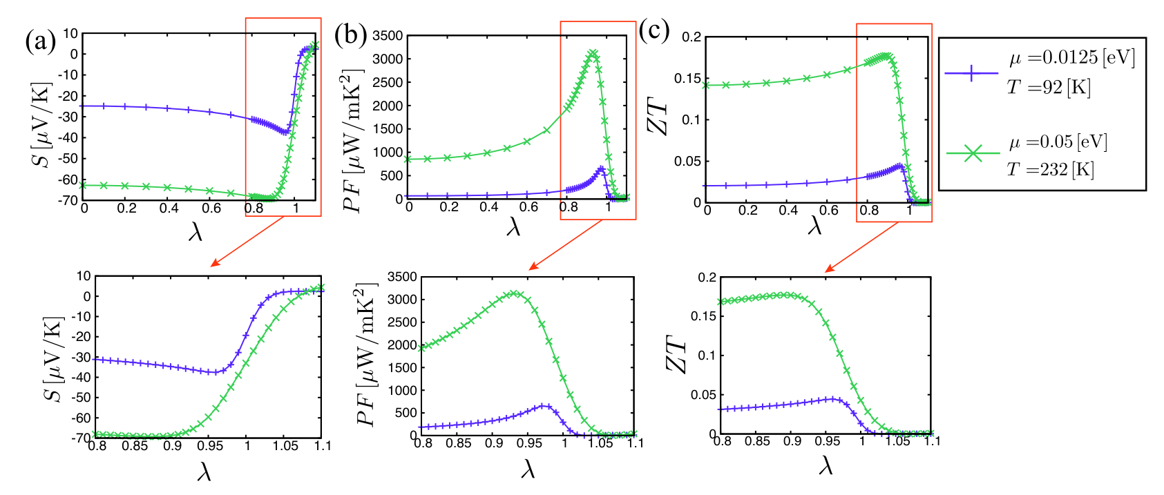
We perform $\epsilon$ integration in Eqs. (7), (18), and (19) numerically, and calculate $S$, PF and $ZT$ by using $L_{11}$, $L_{12}$, and $L_{22}$ thus obtained. In the actual numerical calculation, we limit the interval of the integration to $\epsilon\in[-1,1]$ (eV) in Eqs. (7), (18), and (19), and perform the integration numerically with the number of meshes of $\epsilon$ being 960. In this section, the damping rate $\Gamma$ is set to be $0.02$ eV.

The results are shown in Fig. 5(a)-(f). The eight lines are for the different combinations of $\lambda$ and $\mu$. Note that we do not consider the temperature dependence of $\mu$ but we set it as a parameter. We see that for $\lambda\sim 1$, all three quantities have peaks at temperatures on the order of 100 K. In fact, for $\lambda\leq 1$, $S$, PF, and $ZT$ have a maximum at $T\sim\mu/2k_{\rm B}$. For $S$ and $ZT$, this fact can be accounted for by the linear dependence of $\alpha_{xx}(\epsilon)$ as a function of $\epsilon$; see Appendix B for details.

Among the combinations of $\lambda$ and $\mu$ shown in Fig. 5(d)-(f), the case with $\lambda=0.95$ and $\mu=0.05$ eV exhibits the largest response. The results indicate that there exists an optimal degree of tilting and carrier density to obtain large thermoelectric responses. We also see that, in deep inside the type-II case ($\lambda=1.5$), the thermoelectric response functions are small compared with those for $\lambda\sim 1$. Note that, for the type-II case, a dominant contribution to the Seebeck coefficient comes from the region near the Dirac points; see Appendix C for further details.

To further study the optimal tilting for the large thermoelectric response, we investigate the $\lambda$ dependence of $S$, PF, and $ZT$. The results are shown in Fig. 6(a)-(c). The temperatures are set to be $T=92$ K and $232$ K for $\mu=0.0125$ eV and 0.05 eV, respectively, where the peaks are realized in Fig. 5(d)-(f). We see that the optimal tilting parameter $\lambda$ indeed exists, and is slightly smaller than $\lambda=1$. We also see that, for all of the three quantities, their absolute values for $\mu=0.05$ eV are larger than those for $\mu=0.0125$ eV. However, as we will argue in the next section, they do not increase monotonically as a function of $\mu$. Rather, an optimal value of $\mu$ also exists, as we will explain in the next section. Therefore, for the large thermoelectric response, the suitable electronic structure is the type-I Dirac cone which is very close to the type-III Dirac cone. The carrier density (or the chemical potential) also should also be tuned at the optimal value. At the maximum within the present results ($\mu=0.05$ eV and $\lambda=0.89$), we obtain $S\sim-70\hskip 1.42262pt\mathrm{\mu V}/\mathrm{K}$, PF $\sim 3000\hskip 1.42262pt\mu\mathrm{W}/\mathrm{mK}^{2}$, and $ZT\sim 0.18$, which are sizable values.

To understand the physical origin of the large Seebeck coefficient and large $ZT$, it is useful to study their low-temperature behaviors. To this end, for $L_{12}$, we apply the Sommerfeld expansion to Eq. (18). Then, we find that, for low temperatures, $S$ is given by the Mott formula Mott and Jones 1936,

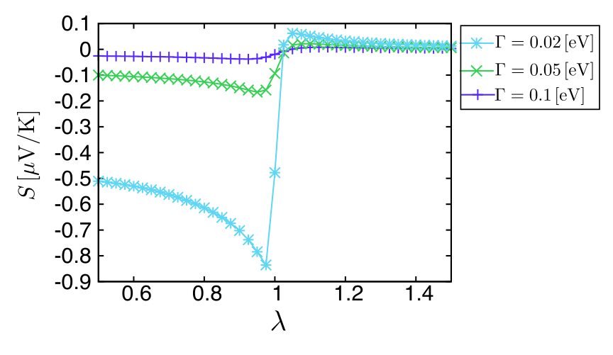
In Fig. 7(a)-(c), we show the $\mu$ dependence of $S$ obtained from the Mott formula for $\mu\in[-0.5,0.5]$ eV. We set the temperature to be small but finite, as $T=1.16$ K (i.e., $k_{\rm B}T=10^{-4}|t|$). We see that $S$ is vanishing when $\mu$ is right at the Dirac point for all the three types, as $S$ is the odd function of $\mu$. Comparing the three types, we find that the type-I and type-III cases have large $S$, while the type-II case has small $S$. This can be accounted for by the fact that the conductivity (or $L_{11}$) is large for the type-II case.

We also find that the sign of $S$ in the type-I and type-III cases is opposite that for the type II case. For instance, for positive $\mu$, $S$ is negative for $\lambda=0.5$ and $1$, while $S$ is positive for $\lambda=1.5$. To further clarify the nature of the sign change, we plot the $\lambda$ dependence of $S$ at $\mu=0.0125$ eV in Fig. 8. As $\lambda$ approaches $1$ from the type-I region, $S$ is negative, and $|S|$ becomes larger. At $\lambda=1$, i.e., the type-III case, $S$ is still negative but $|S|$ decreases. This indicates the non-monotonic behavior of $S$ upon increasing the tilting of the Dirac cones from the type-I side. Then, the sign change of $S$ occurs for $\lambda=\lambda_{\rm c}$ with $\lambda_{\rm c}>1$. Note that this behavior is also seen at finite temperatures, as shown in Fig. 6(a). The result can be understood as follows. From Eqs. (7) and (20), one finds that $S$ is proportional to the $\mu$-derivative of $\sigma$ at $T=0$. Then, the sign of $S$, which is equal to that of $L_{12}$, is dictated by whether $\sigma$ at $\mu=0$ is a dip or a peak. Clearly, types-I and III show a dip, while type-II shows a peak, which coincides with the resulting sign of $S$.

Next, we present the results of the power factor. To estimate the low-temperature behavior, we again employ the Sommerfeld expansion to $L_{12}$. In Fig. 9(a)-(c), we show the $\mu$ dependence of PF. As can clearly be seen, a large power factor is obtained for types I and III for small but finite $\mu$. In particular, the power factor for the type-III Dirac system is the largest among the three types for $\Gamma=0.02,0.05$ eV with $|\mu|\lesssim 0.05$ eV, due to the subtle competition between $L_{12}$ and $L_{11}$.

References

- Wallace (1947) P. R. Wallace, Phys. Rev. 71, 622 (1947).
- Novoselov et al. (2004) K. S. Novoselov, A. K. Geim, S. V. Morozov, D. Jiang, Y. Zhang, S. V. Dubonos, I. V. Grigorieva, and A. A. Firsov, Science 306, 666 (2004).
- Castro Neto et al. (2009) A. H. Castro Neto, F. Guinea, N. M. R. Peres, K. S. Novoselov, and A. K. Geim, Rev. Mod. Phys. 81, 109 (2009).
- Kajita et al. (2014) K. Kajita, Y. Nishio, N. Tajima, Y. Suzumura, and A. Kobayashi, Journal of the Physical Society of Japan 83, 072002 (2014).
- Katayama et al. (2006) S. Katayama, A. Kobayashi, and Y. Suzumura, Journal of the Physical Society of Japan 75, 054705 (2006).
- Kobayashi et al. (2007) A. Kobayashi, S. Katayama, Y. Suzumura, and H. Fukuyama, Journal of the Physical Society of Japan 76, 034711 (2007).
- Fukuyama (2007) H. Fukuyama, Journal of the Physical Society of Japan 76, 043711 (2007).
- Goerbig et al. (2008) M. O. Goerbig, J.-N. Fuchs, G. Montambaux, and F. Piéchon, Phys. Rev. B 78, 045415 (2008).
- Kobayashi et al. (2008) A. Kobayashi, Y. Suzumura, and H. Fukuyama, Journal of the Physical Society of Japan 77, 064718 (2008).
- Kobayashi et al. (2009) A. Kobayashi, Y. Suzumura, H. Fukuyama, and M. O. Goerbig, Journal of the Physical Society of Japan 78, 114711 (2009).
- Volovik (2016) G. E. Volovik, JETP Letters 104, 645 (2016).
- Volovik and Zhang (2017) G. E. Volovik and K. Zhang, Journal of Low Temperature Physics 189, 276 (2017).
- Volovik (2018) G. E. Volovik, Physics-Uspekhi 61, 89 (2018).
- Liu et al. (2018) H. Liu, J.-T. Sun, C. Cheng, F. Liu, and S. Meng, Phys. Rev. Lett. 120, 237403 (2018).
- Huang et al. (2018) H. Huang, K.-H. Jin, and F. Liu, Phys. Rev. B 98, 121110 (2018).
- Fragkos et al. (2019) S. Fragkos, R. Sant, C. Alvarez, E. Golias, J. Marquez-Velasco, P. Tsipas, D. Tsoutsou, S. Aminalragia-Giamini, E. Xenogiannopoulou, H. Okuno, G. Renaud, O. Rader, and A. Dimoulas, Phys. Rev. Materials 3, 104201 (2019).
- Milićević et al. (2019) M. Milićević, G. Montambaux, T. Ozawa, O. Jamadi, B. Real, I. Sagnes, A. Lemaître, L. Le Gratiet, A. Harouri, J. Bloch, and A. Amo, Phys. Rev. X 9, 031010 (2019).
- Farajollahpour et al. (2019) T. Farajollahpour, Z. Faraei, and S. A. Jafari, Phys. Rev. B 99, 235150 (2019).
- Kim et al. (2020) J. Kim, S. Yu, and N. Park, Phys. Rev. Applied 13, 044015 (2020).
- Chen et al. (2020) Y.-G. Chen, X. Luo, F.-Y. Li, B. Chen, and Y. Yu, Phys. Rev. B 101, 035130 (2020).
- Jin et al. (2020a) L. Jin, H. C. Wu, B.-B. Wei, and Z. Song, Phys. Rev. B 101, 045130 (2020a).
- Gong et al. (2020) Z. Gong, X. Shi, J. Li, S. Li, C. He, T. Ouyang, C. Zhang, C. Tang, and J. Zhong, Phys. Rev. B 101, 155427 (2020).
- Jin et al. (2020b) L. Jin, X. Zhang, Y. Liu, X. Dai, L. Wang, and G. Liu, Phys. Rev. B 102, 195104 (2020b).
- Farajollahpour and Jafari (2020) T. Farajollahpour and S. A. Jafari, Phys. Rev. Research 2, 023410 (2020).
- Fragkos et al. (2021) S. Fragkos, P. Tsipas, E. Xenogiannopoulou, Y. Panayiotatos, and A. Dimoulas, Journal of Applied Physics 129, 075104 (2021).
- Li et al. (2021) X.-P. Li, K. Deng, B. Fu, Y. Li, D.-S. Ma, J. Han, J. Zhou, S. Zhou, and Y. Yao, Phys. Rev. B 103, L081402 (2021).
- Sims (2021) C. Sims, Condensed Matter 6, 18 (2021).
- Suzumura et al. (2014a) Y. Suzumura, I. Proskurin, and M. Ogata, Journal of the Physical Society of Japan 83, 023701 (2014a).
- Suzumura et al. (2014b) Y. Suzumura, I. Proskurin, and M. Ogata, Journal of the Physical Society of Japan 83, 094705 (2014b).
- Proskurin et al. (2015) I. Proskurin, M. Ogata, and Y. Suzumura, Phys. Rev. B 91, 195413 (2015).
- Mani and Benjamin (2017) A. Mani and C. Benjamin, Phys. Rev. E 96, 032118 (2017).
- Mani and Benjamin (2019) A. Mani and C. Benjamin, The Journal of Physical Chemistry C 123, 22858 (2019).
- Mani et al. (2019) A. Mani, S. Pal, and C. Benjamin, Scientific Reports 9, 6018 (2019).
- Koshino and Ando (2007) M. Koshino and T. Ando, Phys. Rev. B 76, 085425 (2007).
- Koshino and Ando (2010) M. Koshino and T. Ando, Phys. Rev. B 81, 195431 (2010).
- Gómez-Santos and Stauber (2011) G. Gómez-Santos and T. Stauber, Phys. Rev. Lett. 106, 045504 (2011).
- Raoux et al. (2015) A. Raoux, F. Piéchon, J.-N. Fuchs, and G. Montambaux, Phys. Rev. B 91, 085120 (2015).
- Ogata (2016) M. Ogata, Journal of the Physical Society of Japan 85, 104708 (2016).
- Ferreiros et al. (2017) Y. Ferreiros, A. A. Zyuzin, and J. H. Bardarson, Phys. Rev. B 96, 115202 (2017).
- Kozii et al. (2019) V. Kozii, B. Skinner, and L. Fu, Phys. Rev. B 99, 155123 (2019).
- Rostamzadeh et al. (2019) S. Rostamzadeh, i. d. I. m. c. Adagideli, and M. O. Goerbig, Phys. Rev. B 100, 075438 (2019).
- Mawrie and Muralidharan (2019) A. Mawrie and B. Muralidharan, Phys. Rev. B 100, 081403 (2019).
- Mandal and Saha (2020) I. Mandal and K. Saha, Phys. Rev. B 101, 045101 (2020).
- Ohki et al. (2020) D. Ohki, Y. Omori, and A. Kobayashi, Phys. Rev. B 101, 245201 (2020).
- McCormick et al. (2017a) T. M. McCormick, I. Kimchi, and N. Trivedi, Phys. Rev. B 95, 075133 (2017a).
- McCormick et al. (2017b) T. M. McCormick, R. C. McKay, and N. Trivedi, Phys. Rev. B 96, 235116 (2017b).
- McKay et al. (2019) R. C. McKay, T. M. McCormick, and N. Trivedi, Phys. Rev. B 99, 245119 (2019).
- Mizoguchi and Hatsugai (2020) T. Mizoguchi and Y. Hatsugai, Journal of the Physical Society of Japan 89, 103704 (2020).
- Kubo (1957) R. Kubo, Journal of the Physical Society of Japan 12, 570 (1957).
- Luttinger (1964) J. M. Luttinger, Phys. Rev. 135, A1505 (1964).
- Hwang et al. (2007) E. H. Hwang, S. Adam, and S. D. Sarma, Phys. Rev. Lett. 98, 186806 (2007).
- Hwang et al. (2009) E. H. Hwang, E. Rossi, and S. Das Sarma, Phys. Rev. B 80, 235415 (2009).
- Mahan (1990) G. D. Mahan, Many-Particle Physics (Plenum, New York, 1990).
- Yamamoto and Fukuyama (2018) T. Yamamoto and H. Fukuyama, Journal of the Physical Society of Japan 87, 024707 (2018).
- Ogata and Fukuyama (2019) M. Ogata and H. Fukuyama, Journal of the Physical Society of Japan 88, 074703 (2019).
- Jacimovski et al. (2015) S. K. Jacimovski, M. Bukurov, J. P. Setrajcic, and D. I. RakoviC, Superlattices and Microstructures 88, 330 (2015).
- Jonson and Mahan (1980) M. Jonson and G. D. Mahan, Phys. Rev. B 21, 4223 (1980).
- Kontani (2003) H. Kontani, Phys. Rev. B 67, 014408 (2003).
- Sommerfeld and Bethe (1933) A. Sommerfeld and H. Bethe, Elektronentheorie der Metalle, Handbuch der Physik, Vol. 24/2 (Springer, Berlin/Heidelberg, 1933).
- Matsuura et al. (2019) H. Matsuura, H. Maebashi, M. Ogata, and H. Fukuyama, Journal of the Physical Society of Japan 88, 074601 (2019).
- Mott and Jones (1936) N. F. Mott and H. Jones, The Theory of the Properties of Metals and Alloys (Dover New York, 1936).
- Inokuchi et al. (1995) M. Inokuchi, H. Tajima, A. Kobayashi, T. Ohta, H. Kuroda, R. Kato, T. Naito, and H. Kobayashi, Bulletin of the Chemical Society of Japan 68, 547 (1995).
- Tsumuraya and Suzumura (2021) T. Tsumuraya and Y. Suzumura, Eur. Phys. J. B 94, 17 (2021).
- Kitou et al. (2021) S. Kitou, T. Tsumuraya, H. Sawahata, F. Ishii, K.-i. Hiraki, T. Nakamura, N. Katayama, and H. Sawa, Phys. Rev. B 103, 035135 (2021).
- Konoike et al. (2013) T. Konoike, M. Sato, K. Uchida, and T. Osada, Journal of the Physical Society of Japan 82, 073601 (2013).
- (66) R. Kitamura, N. Tajima, K. Kajita, R. Kato, M. Tamura, T. Naito, and Y. Nishio, Proceedings of the 12th Asia Pacific Physics Conference (APPC12) 1, 012097.
- Kobayashi et al. (2004) A. Kobayashi, S. Katayama, K. Noguchi, and Y. Suzumura, Journal of the Physical Society of Japan 73, 3135 (2004).
- Kishigi and Hasegawa (2017) K. Kishigi and Y. Hasegawa, Phys. Rev. B 96, 085430 (2017).
- Mahan and Sofo (1996) G. D. Mahan and J. O. Sofo, Proceedings of the National Academy of Sciences 93, 7436 (1996).
- Hasdeo et al. (2019) E. H. Hasdeo, L. P. A. Krisna, M. Y. Hanna, B. E. Gunara, N. T. Hung, and A. R. T. Nugraha, Journal of Applied Physics 126, 035109 (2019).