From inexact optimization to learning via gradient concentration
Abstract
Optimization in machine learning typically deals with the minimization of empirical objectives defined by training data. However, the ultimate goal of learning is to minimize the error on future data (test error), for which the training data provides only partial information. In this view, the optimization problems that are practically feasible are based on inexact quantities that are stochastic in nature. In this paper, we show how probabilistic results, specifically gradient concentration, can be combined with results from inexact optimization to derive sharp test error guarantees. By considering unconstrained objectives we highlight the implicit regularization properties of optimization for learning.
1 Introduction
Optimization plays a key role in modern machine learning, and is typically used to define estimators by minimizing empirical objective functions [SNW11]. These objectives are based on a data fit term, suitably penalized, or constrained, to induce an inductive bias in the learning process [SSBD14]. The idea is that the empirical objectives should provide an approximation to the error on future data (the test error) which is the quantity that one wishes to minimize in learning. The quality, of such an approximation error is typically deferred to a statistical analysis. In this view, optimization and statistical aspects are tackled separately.
Recently, a new perspective has emerged in machine learning showing that optimization itself can in fact be directly used to search for a solution with small test error. Interestingly, no explicit penalties/constraints are needed, since a bias in the search for a solution is implicitly enforced during the optimization process. This phenomenon has been called implicit regularization and it has been shown to possibly play a role in explaining the learning curves observed in deep learning, see for instance in [GLSS18, Ney17] and references therein. Further, implicit regularization has been advocated as a way to improve efficiency of learning methods by tackling statistical and optimization aspects at once [RV15, YWW19, BHR18, CW21]. As it turns out, implicit regularization is closely related to the notion of iterative regularization with a long history in inverse problems [Lan51].
The basic example of implicit regularization is gradient descent for linear least squares, which is well known to converge to the minimum norm least squares solution [EHN96, YCR07]. The learning properties of gradient descent for least squares are now quite well understood [YCR07, RYW14] including the extension to non-linear kernelized models [BPR07, BM18], stochastic gradients [DFB17, DB16, MNR19], accelerated methods [BK16, PR19] and distributed approach-es [ZDW15, MB18, RR20]. Much less is known when other norms or loss functions are considered. Implicit regularization biased to more general norms have been considered for example in [VKR20, VMVR17]. Implicit regularization for loss functions other than the square loss have been considered in a limited number of works. There is a vast literature on stochastic gradients techniques, see e.g. [MNR19] and references therein, but these analyses do not apply when (batch) training error gradients are used, which is the focus in this work. The logistic loss functions for classification has recently been considered both for linear and non-linear models, see for example [SHN+18, JT19]. Implicit regularization for general convex Lipchitz loss with linear and kernel models have been first considered in [LRZ16] for subgradient methods and in [LCR16] for stochastic gradient methods but only with suboptimal rates. Improved rates have been provided in [YWW19] for strongly convex losses and more recently in [LHT21] with a general but complex analysis. A stability based approach, in the sense of [BE02], is studied in [CJY18].
In this paper, we further push this line of work considering implicit regularization for linear models with convex, Lipschitz and smooth loss functions based on gradient descent. Indeed, for this setting we derive sharp rates considering both the last and the average iterate. Our approach highlights a proof technique which is less common in learning and is directly based on a combination of optimization and statistical results. The usual approach in learning theory is to derive optimization results for empirical objectives and then use statistical arguments to asses to which extent the empirical objectives approximate the test error that one ideally wished to minimize, see e.g. [SSBD14]. Instead, we view the empirical gradient iteration as the inexact version of the gradient iteration for the test error. This allows to apply results from inexact optimization, see e.g.[BT00, SRB11], and requires using statistical/probabilistic arguments to asses the quality of the gradient approximations (rather than that of the objectives functions). For this latter purpose, we utilize recent concentration of measures results for vector valued variables, to establish gradient concentration [FSS18]. While the idea of combining inexact optimization and concentration results has been considered before [GDG20], here we illustrate it in a prominent way to highlight its usefulness. Indeed, we show that this approach leads to sharp results for a specific but important setting and we provide some simple numerical results that illustrate and corroborate our findings. By highlighting the key ideas in the proof techniques we hope to encourage further results combining statistics and optimization, for example considering other forms of gradient approximation or optimization other than the basic gradient descent.
The remainder of the paper is structured as follows: In Section 2, we collect some structural assumptions for our setting. In Section 3, we formulate the assumptions we put on the loss function and state and discuss the main results of the paper and the novel aspects of our approach. Section 4 presents the more technical aspects of the analysis. In particular, we explain in detail how results from inexact optimization and concentration of measure can be combined to come up with a new proof technique for learning rates. Finally, Section 5 illustrates the key features of our theoretical results with numerical experiments.
2 Learning with gradient methods and implicit regularization
Let be a real, separable Hilbert space and a subset of . We consider random variables on a probability space with values in and unknown distribution . The marginal distribution of is denoted by . Additionally, we make the standard assumption that is bounded.
- (A1)
(Bound): We assume almost surely for some .
Based on the observation of i.i.d. copies of , we want to learn a linear relationship between and expressed as an element .11 1 Note that this includes many settings as special instances. In particular, it includes the standard setting of kernel learning, see Appendix A in [RV15]. For an individual observation and the choice , we suffer the loss , where is a product-measurable loss function. Our goal is to find such that that the population risk given by
| (2.1) |
is small. The observed data represent the training set, while the population risk can be interpreted as an abstraction of the concept of the test error.
In the following, we assume that a minimizer of in exists.
- (A2)
(Min): We assume there exists some such that .
Note that the is taken only over and not over all measurable functions. Under (Min), minimizing the population risk is equivalent to minimizing the excess risk .
In this work, we are interested in bounding the excess risk, when our choice of is based on applying gradient descent (GD) to the empirical risk computed from the training data,
| (2.2) |
We consider a basic gradient iteration, which is well defined when the loss function is differentiable in the second argument with a product-measurable derivative .
Definition 2.1 (Gradient descent algorithm).
- 1.
Choose and a sequence of step sizes .
- 2.
For , define the GD-iteration
(2.3) - 3.
For some , we consider both the last iterate and the the averaged GD-iterate .
Here, we focus on batch gradient, so that all training points are used in each iteration. Unlike with stochastic gradient methods, the gradients at different iterations are not conditionally independent. Indeed, the analysis of batch gradient is quite different to that of stochastic gradient and could be a first step towards considering minibatching [LR17, MNR19, GDG20]. In our analysis, we always fix a constant step size for all and consider both the average and last iterate. Both choices are common in the optimization literature [SNW11] and have also been studied in the context of learning with least squares [DB16, BM18, MNR19], see also our extended discussion in Subsection 3.2. In the following, we characterize the learning properties of the gradient iteration in Definition 2.1 in terms of the corresponding excess risk. In particular, we derive learning bounds matching the best bounds for estimators obtained minimizing the penalized empirical risk. Next, we show that in the considered setting learning bounds can be derived by studying suitable bias and variance terms controlled by the iteration number and the step size.
3 Main results and discussion
Before stating and discussing our main results, we introduce and comment on the basic assumptions needed in our analysis. We make the following additional assumptions on the loss function.
- (A3)
(Conv): We assume is convex in the second argument.
- (A4)
(Lip): We assume to be -Lipschitz, i.e. for some ,
(3.1) - (A5)
For notational convenience, we state the assumptions (Lip) and (Smooth) globally for all . It should be noted, however, that this is not necessary.
Remark 3.1 (Local formulation of assumptions).
In light of Remark 3.1 our analysis is applicable to many widely used loss functions, see e.g. Chapter 2 in [SC08].
Example 3.2 (Loss functions satisfying the assumptions).
- (a)
(Squared loss): If for some , then checking first and second derivatives yields that the loss is convex, -Lipschitz with constant and -Smooth with constant .
- (b)
(Logistic loss for regression): If , then, analogously, the loss is convex, L-Lipschitz with constant and -smooth with constant .
- (c)
(Logistic loss for classification): For classification problems with , analogously, the loss is convex, -Lipschitz with constant and -Smooth with constant .
- (d)
(Exponential loss): For classification problems with , analogously, the loss is convex, -Lipschitz with constant and -smooth also with .
Under Assumption (Smooth), the empirical risk is differentiable and we have
| (3.4) |
With Assumptions (Bound) and (Lip), via dominated convergence, the same is true for the expected risk and we have
| (3.5) |
Further, our assumptions on the loss directly translate into properties of the risks:
- (A3’)
(R-Conv): Under (Conv), both the expected and the empirical risk are convex.
- (A4’)
- (A5’)
The derivation, which is straightforward, is included in Lemma A.1 in Appendix A.
3.1 Formulation of main results
A first key result shows that, under the above assumptions, we can decompose the excess risk for the averaged GD-iterate as well as for the last iterate .
Proposition 3.3 (Decomposition of the excess risk).
The proof of Proposition 3.3 can be found in Appendix A. The above decomposition is derived using ideas from inexact optimization, in particular results studying inexact gradients see e.g. [BT00, SRB11]. Indeed, our descent procedure can be regarded as one in which the population gradients are perturbed by the gradient noise terms
| (3.6) |
We further develop this discussion in Section 4.1.
Note that the results above apply to any . Later we will of course set from Assumption (Min). With this choice, Proposition 3.3 (i) and (ii) provide decompositions of the excess risk into a deterministic bias part
| (3.7) |
which can be seen as an optimization error, and a stochastic variance part, which is an average of the terms
| (3.8) |
Note that Proposition 3.3 (i) can be applied to the first sum on the right-hand side in (ii). In order to control the bias part, it is sufficient to choose large enough. Controlling the variance part is more subtle and requires some care. By Cauchy-Schwarz inequality,
| (3.9) |
A similar estimate holds for the terms , . This shows that in order to upper bound the excess risk of the average gradient iteration it is sufficient to solve two problems:
- 1.
Bound the gradient noise terms in norm;
- 2.
Bound the gradient path in a ball around .
Starting from this observation, in Proposition 4.4, we state a general gradient concentration result which, for fixed , allows to derive
| (3.10) |
with high probability in when is sufficiently large. If we could prove that the gradient path stays bounded, this would allow to control the gradient noise terms. However, the result in Equation (3.10) itself is not enough to directly derive a bound for the gradient path. Indeed, in Proposition 4.6, we show how gradient concentration can be used to inductively prove that with high probability stays bounded by for sufficiently large. Importantly, gradient concentration thereby allows to control the generalization error of the excess risk and the deviation of the gradient path at the same time. This makes this proof technique particularly appealing comparative to other approaches in the literature, see the discussion in Sections 3.2 and 4. Taken together, the arguments above are sufficient to prove sharp rates for the excess risk.
Theorem 3.4 (Excess Risk).
The proof of Theorem 3.4 is in Appendix A. Here, we comment on the above result. The gradient concentration inequality allows to derive an explicit estimate for the variance. As expected, the latter improves as the number of samples increases, but interestingly it stays bounded, provided that is not too large, see Equation (3.11). Optimizing the choice of leads to the final excess risk bound. Such an estimate is sharp in the sense that it matches the best available bounds for other estimation schemes based on empirical risk minimization with penalties, see e.g. [SSBD14, SC08] and references therein. We note that the average and last iterates have essentially the same performance, up to constants and logarithmic terms.
It is worth noting that a number of different choices for the stopping time and the step size are possible, as long as their product stays constant. Assuming that from (Bound) is known, the user may choose the step size a priori when from (Smooth) is known, see Example 3.2 (a), (b), (c). When depends on the bound , see Proposition 4.6, the choice of must be adapted to the norm of the minimizer , see e.g. Example 3.2 (d) and the discussion in Remark 3.1. In this sense, it is indeed the product that plays the role of a regularization parameter, see also Figure 1 in Section 5.
The excess risk bound in the above theorem matches the best bound for least squares, obtained with an ad hoc analysis [YCR07, RYW14]. The obtained bound improves the results obtained in [LRZ16] and recovers the results in [LHT21] in a special case. Indeed, these latter results are more general and allow to derive fast rates, however this generality is payed in terms of a considerably more complex analysis. In particular, our analysis allows to get explicit constants and keep the step size constant. More importantly, the proof we consider follows a different path, highlighting the connection to inexact optimization. We further develop this point of view next.
3.2 Discussion of related work
Comparison to the classical approach. In order to better locate our work in the machine learning and statistical literature, we compare it with the most important related line of research.
In particular, we contrast our approach with the one typically used to study learning with gradient descent and general loss functions. We briefly review this latter and more classical approach. The following decomposition is often considered to decompose the excess risk at :
| (3.12) |
see e.g. [SSBD14, BB11]. The second term in the decomposition can be seen as an optimization error and treated by deterministic results from ”exact” optimization. The first and last terms are stochastic and are bounded using probabilistic tools. In particular, the first term, often called generalization error, needs some care. The two more common approaches are based on stability, see e.g. [BE02, CJY18], or empirical process theory [BLM13], [SC08]. Indeed this latter approach is the one considered in [LRZ16, LHT21]. In this case, the key quantity is the empirical process defined as,
| (3.13) |
To study the latter, a main complication is that the iterates norm/path needs be bounded almost surely, and indeed this is a delicate point, as discussed in detail in Section 4.2. In our approach, gradient concentration allows to find a sharp bound on the gradient path and at the same time to directly derive an excess risk bound, avoiding the decomposition in (3.12) and further empirical process bounds.
Inexact optimisation and gradient concentration.
We are not the first to employ tools from inexact optimisation
to treat learning problems, see [BWY17] and
[YWW19].
A similar decomposition as in
Proposition 3.3 together with a peeling
argument instead of gradient concentration is used in [YWW19].
The authors, however, derive a bound for a ”conditional excess risk”.
More specifically, the risk is the conditional expectation, conditioned on the
covariates, and is thus still a random quantity.
The minimizer considered is the minimizer with respect to this random risk and
therefore is a random quantity too.
Additionally, their analysis requires strong convexity of the conditional risk
with respect to the empirical norm.
Our approach allows to overcome these two restrictions.
Also gradient concentration has been considered before, see e.g. [HI18, PSBR18].
In particular, in [HI18] an analysis is developed under the assumption that minimization of the risk is constrained over a
closed, convex and bounded set , effectively considering an explicit regularization.
During their gradient iteration, a projection step is then considered to enforce such a constraint.
As a consequence the dimension and the diameter of appear as key
quantities that determine the error behavior of their algorithm.
The same is essentially true for [PSBR18].
In comparison, our analysis is dimension free. More importantly, however, we do not
consider any constraint, hence considering implicit, rather than explicit, regularization.
Also, from a technical point of view this is a key difference. As we discuss in Section 4.2 bounding the gradient path is required, in the absence of explicit constraints.
The main contribution of our paper, as we see it, is to show that the
combination of optimisation and concentration of measure techniques presented
allow to seamlessly control the excess risk and the length of the gradient
path at the same time, whereas in other analyses, e.g.
[LHT21], these two tasks have to be separated and are
much more involved.
Finally, we discuss in detail the results in [GDG20], of which
we had not been aware after finishing this work and are closely related.
Indeed, also in this paper inexact optimization and gradient concentration are combined, albeit in a different way.
In Theorem G.1., the authors consider stochastic gradient descent for a convex
and smooth objective function on , notably also on an
unbounded domain.
For their analysis, they introduce clipped versions of the stochastic
gradients.
They also borrow a decomposition of the excess risk from inexact optimization,
although a different one.
In particular, it is not straightforward that their decomposition would also
yield results for the last gradient iteration.
In a second step, they then use the conditional independence of gradient
batches and a Bernstein-type inequality for Martingale differences
to derive concentration for several terms involving gradient noise terms.
In comparison, instead of concentration based on individual batches, we use the
full empirical gradients together with a uniform concentration result based on
Rademacher complexities of Hilbert space valued function classes, see Section
4.2.
On the one hand, our setting is more general, since we consider a Hilbert
space instead of .
On the other hand, [GDG20] are notably able to
forgo property (R-Lip), i.e.
their gradients can be unbounded.
This is the main aspect of their analysis.
As a consequence their result is tailored to this setting
and does not contain ours as a special case.
In particular, with property
(R-Lip),
even on , our result is much sharper.
We avoid an additional -factor and, more importantly, we are able to
freely choose a large, fixed step size .
In Theorem G.1. of [GDG20], the step size has to depend both on the number of iterations
and the high probability guarantee of the result.
Further, our results in Theorem 3.4 are particularly sharp
with explicit constants and one clear regularization parameter, , that can, in principle, be chosen via sample splitting and early
stopping.
Conversely, in order to control the unbounded gradients
[GDG20]
have to introduce two additional hyperparameters:
the gradient clipping threshold and the batch size .
In their analysis, both of these have to be chosen in dependence of the true
minimizer.
In particular, the clipping threshold de facto regularizes the
problem based on a priori knowledge of the true solution, very much in the way
as a bounded domain would. Developing these observations is indeed an interesting venue for further research.
Last iterate vs. averaged iterates convergence. Finally, we compare our results to other high probability bounds for gradient descent. High probability bounds for both last iterate and (tail-)averaged gradient convergence with constant stepsize for least squares regression in Hilbert spaces are well established. Indeed, the former follows from [BM18, LRRC20] as gradient descent belongs to the broader class of spectral regularisation methods. Note that this also is well known in the context of inverse problems, see e.g. [EHN96]. As observed in [MNR19], also average gradient descent can be cast and analyzed in the spectral filtering framework. Indeed, average and last iterates can be seen to share essentially the same excess risk bound. However, the proof is heavily tailored to least squares. Compared to these results, for smooth losses, we establish a high probability bound of order for uniform averaging and for last iterate GD, for any sufficiently large, with constant stepsize, only worse by a factor of . We note that, it was shown in [HLPR19] that the factor is in fact necessary for Lipschitz functions for last iterate SGD and GD with decaying stepsizes. Indeed, the authors derive a sharp high probability bound of order for last iterate (S)GD, while uniform averaging achieves a faster rate of . Notably, this work even shows the stronger statement: Any convex combination of the last iterates must incur a factor. Finally, we note that [LRZ16] derive finite sample bounds for subgradient descent for convex losses, considering the last iterate. In this work, early stopping gives a suboptimal rate, with decaying stepsize and also an additional logarithmic factor. This vanishes under additional differentiability and smoothness for constant stepsize.
4 From inexact optimization to learning
In this section, we further discuss the important elements of the proof. The alternative error decomposition we presented in Proposition 3.3 follows from taking the point of view of optimization with inexact gradients [BT00]. The idea is to consider an ideal GD-iteration subject to noise, i.e.
| (4.1) |
where, the are gradient noise terms. In Equation (4.1), very general choices for may be considered. Clearly, in our setting, we have
| (4.2) |
From this perspective, the empirical GD-iteration can be seen as performing gradient descent directly on the population risk, however, the gradient is corrupted with noise and convergence has to be balanced out with a control of the stability of the iterates. Next, we see how these ideas can be applied to the learning problem.
4.1 Inexact gradient descent
From the point of view discussed above, it becomes essential to relate both the risk and the norm of a fixed GD-iteration to the gradient noise. In the following, we provide two technical Lemmas, which do exactly that. Both results could also be formulated for general gradient noise terms . For the sake of simplicity, however, we opt for the more explicit formulation in terms of the gradients. The proofs are based on entirely deterministic arguments and can be found in Appendix B.
Lemma 4.1 (Inexact gradient descent: Risk).
Lemma 4.1 is the key component to obtain the decomposition of the excess risk in Proposition 3.3 for the averaged GD-iteration. This online to batch conversion easily follows by exploiting the convexity of the population risk (R-Conv).
The next Lemma is crucial in providing a high probability guarantee for the boundedness of the gradient path in Proposition 4.6, which is necessary to apply gradient concentration to the decomposition of the excess risk in Proposition 3.3.
Lemma 4.2 (Inexact gradient descent: Gradient path).
4.2 Gradient concentration
In this section, we discuss how the gradient concentration inequality in Equation (3.10) is derived using results in [FSS18]. We use a gradient concentration result which is expressed in terms of the Rademacher complexity of a function class defined by the gradients with
| (4.4) |
Since the gradients above are elements of the Hilbert space , the notion of Rademacher complexities has to be stated for Hilbert space-valued function classes, see [Mau16].
Definition 4.3 (Rademacher complexities).
Let be a real, separable Hilbert space. Further, let be a class of maps and be a vector of i.i.d. random variables. We define the empirical and population Rademacher complexities of by
| (4.5) |
respectively, where is a vector of i.i.d. Rademacher random variables independent of .
In our setting, we consider . Fix some and consider the scalar function class
| (4.6) |
and more importantly, the -valued, composite function class
| (4.7) |
Under (Bound) and (Lip), we have
| (4.8) |
where denotes the -norm on the underlying probability space .
The gradient concentration result can now be formulated in terms of the empirical Rademacher complexity of .
Proposition 4.4 (Gradient concentration).
The proof of Proposition 4.4 is stated in Appendix B. To apply Proposition 4.4, we need to bound . This can be done relating the empirical Rademacher complexity of the composite function class back to the complexity of the scalar function class .
Lemma 4.5 (Bounds on the empirical Rademacher complexities).
Note that since the bounds in Lemma 4.5 do not depend on the sample , they also hold for the population Rademacher complexities. Lemma 4.5 (i) is a classic result, which we restate for completeness. Lemma 4.5 (ii) is more involved and requires combining a vector-contraction inequality from [Mau16] with additional more classical contraction arguments to disentangle the concatenation in the function class . The proof of Lemma 4.5 is stated in Appendix B. Note that the arguments for both Proposition 4.4 and Lemma 4.5 are essentially contained in [FSS18]. Here, we provide a self-contained derivation for our setting.
Together with Lemma 4.2, the gradient concentration result provides an immediate high probability guarantee for the gradient path not to diverge too far from the minimizer .
Proposition 4.6 (Bounded gradient path).
The proof of Proposition 4.6 is stated in Appendix B. In a learning setting, bounding the gradient path is essential to the analysis of gradient descent based estimation procedures. Either one has to guarantee its boundedness a priori, e.g. by projecting back onto a ball of known radius or making highly restrictive additional assumptions, see [LT18], or one has to make usually involved arguments to guarantee its boundedness up to a sufficiently large iteration number, see e.g. [LHT21] and [YWW19]. Our numerical illustration in Figure 1 shows that from a practical perspective, such a boundedness result is indeed necessary to control the variance. Additionally, if the boundedness of the gradient path was already controlled by the optimization procedure for arbitrarily large iterations , then the decomposition in Proposition 3.3 together with our gradient concentration result in Proposition 4.4 would guarantee that for , the deterministic bias part vanishes completely, while the stochastic variance part
| (4.10) |
would remain of order independently of . This would suggest that for large there is no tradeoff between reducing the bias of the estimation method and its variance anymore, which, in that form, should be surprising for learning, see discussion in [DSH20]. From this perspective, in order to analyze gradient descent for learning, it seems needed to establish a result like Proposition 4.6.
We compare our result in Proposition 4.6 with the corresponding result in [LHT21], which is the most recent in the literature. Under the self-boundedness assumption
| (4.11) |
they relate the stochastic gradient descent iteration to the Tikhonov regularizer , whose norm can be controlled and obtain a uniform bound over of the form
| (4.12) |
with high probability in . Later, the risk quantities in Equation (4.12) are related to the approximation error of a kernel space, which guarantees that the stochastic gradient path is sufficiently bounded. For the bound in Equation (4.12), [LHT21] have to choose a decaying sequence of step sizes with . In comparison, the result in Proposition 4.6 allows for a fixed step size . Since sharp rates essentially require that is of order , we may therefore stop the algorithm earlier. In this regard, our result is a little sharper. At the same time, the result in [LHT21] is more general. In fact, under a capacity condition, the authors adapt the bound in Equation (4.12) to allow for fast rates. However, both the proof of Equation (4.12) and its adaptation to the capacity dependent setting are very involved and quite technical. In comparison, Proposition 4.6 is an immediate corollary of Proposition 4.4. In particular, if under additional assumptions, a sharper concentration result for the gradients is possible, our proof technique would immediately translate this to the bound on the gradient path that is needed to guarantee this sharper rate for the excess risk. Indeed, we think these ideas can be fruitfully developed to get new improved results.
5 Numerics
In this section, we provide some empirical illustration to the effects described in Section 3 and Section 4. In particular, we choose the logistic loss for regression from Example 3.2 (b) and concentrate on two aspects: The (un)bounded gradient path for the averaged iterates and the interplay between step size and stopping time. Our experiments are conducted on synthetic data with dimensions, generated as follows: We set the covariance matrix as a diagonal matrix with entries , and choose , with . We generate training data, where the covariates are drawn from a Gaussian distribution with zero mean and covariance . For , the labels follow the model with being standard Gaussian noise. Each experiment is repeated times and we report the average.
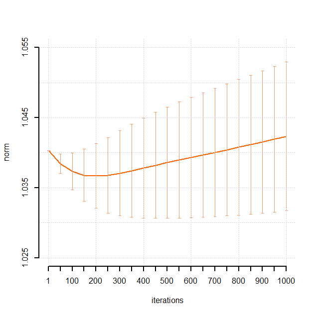
Our first experiment illustrates the behavior of the path for and . As Proposition 4.6 suggest, this path becomes unbounded if the number of iterations grows large.
In a second experiment, we choose a grid of step sizes and stopping times and report the average excess test risk with test data. The result is presented in the right plot in Figure 1. As Theorem 3.4 predicts, for fixed , the performance of averaged GD remains roughly constant as remains constant.

6 Conclusion
In this paper, we studied implicit/iterative regularization for linear, possibly infinite dimensional,
linear models, where the error cost is a convex, differentiable loss function. Our main contribution is a
sharp high probability bound on the excess risk of the averaged and last iterate of batch gradient descent.
We derive these results combining ideas and results from optimization and statistics. Indeed, we show how it is
possible to leverage results from inexact optimization together with concentration inequalities for vector valued functions.
The theoretical results are illustrated to see how the step size and the iteration number control the bias and the stability of the solution.
A number of research directions can further be developed.
In our study we favored a simple analysis to illustrate the main ideas, and as a consequence our results are limited to a basic setting. Indeed, it would be interesting to develop the analysis we presented to get faster learning rates under further assumptions,
for example considering capacity conditions or even finite dimensional models. Another possible research direction is to consider less
regular loss functions, in particular dropping the differentiability assumption. Along similar lines it would be interesting to consider other form of implicit bias or non linear models.
Finally, it would be interesting to consider other forms of optimization including stochastic and accelerated methods.
Acknowledgements
The authors would like to thank Silvia Villa and Francesco Orabona for useful discussions.
The research of B.S. has been partially funded by the Deutsche Forschungsgemeinschaft (DFG)- Project-ID 318763901 - SFB1294.
N.M. acknowledges funding by the Deutsche Forschungsgemeinschaft (DFG) under Excellence Strategy The Berlin Mathematics Research Center MATH+ (EXC-2046/1, project ID:390685689).
L.R. acknowledges support from the Center for Brains, Minds and Machines (CBMM), funded by NSF STC award CCF-1231216. L.R. also acknowledges the financial support of the European Research Council (grant SLING 819789), the AFOSR projects FA9550-18-1-7009, FA9550-17-1-0390 and BAA-AFRL-AFOSR-2016-0007 (European Office of Aerospace Research and Development), and the EU H2020-MSCA-RISE project NoMADS - DLV-777826.
References
- [BB11] L. Bottou and O. Bousquet. The tradeoffs of large scale learning. In Optimization for Machine Learning, pages 351–368. MIT Press, 2011.
- [BE02] Olivier Bousquet and André Elisseeff. Stability and generalization. Journal of Machine Learning Research, 2(Mar):499–526, 2002.
- [BHR18] G. Blanchard, M. Hoffmann, and M. Reiß. Early stopping for statistical inverse problems via truncated SVD estimation. Electronic Journal of Statistics, 12(2):3204–3231, 2018.
- [BK16] G. Blanchard and N. Krämer. Convergence rates of kernel conjugate gradient for random design regression. Analysis and Applications, 14(06):763–794, 2016.
- [BLM13] S. Boucheron, G. Lugosi, and P. Massart. Concentration inequalities: A nonasymptotic theory of independence. Oxford university press, 2013.
- [BM02] P. L. Bartlett and S. Mendelson. Rademacher and Gaussian complexities: Risk bounds and structural results. The Journal of Machine Learning Research, 3:463–482, 2002.
- [BM18] G. Blanchard and N. Mücke. Optimal rates for regularization of statistical inverse learning problems. Foundations of Computational Mathematics, 18:971–1013, 2018.
- [BPR07] F. Bauer, S. Pereverzev, and L. Rosasco. On regularization algorithms in learning theory. Journal of Complexity, 23(1):52–72, 2007.
- [BT00] D. P. Bertsekas and J. N. Tsitsiklis. Gradient convergence in gradient methods with errors. SIAM Journal on Optimization, 10(3):627–642, 2000.
- [Bub15] S. Bubeck. Convex optimization: Algorithms and complexity. Foundations and Trends in Machine Learning, 8(3–4):231–357, 2015.
- [BWY17] S. Balakrishnan, M.J. Wainwright, and B. Yu. Statistical guarantees for the em algorithm: From population to sample-based analysis. The Annals of Statistics, 45(1):77–120, 2017.
- [CJY18] Y Chen, C. Jin, and B. Yu. Stability and convergence trade-off of iterative optimization algorithms, 2018.
- [CW21] A. Celisse and M. Wahl. Analyzing the discrepancy principle for kernelized spectral filter learning algorithms. Journal of Machine Learning Research, 22(76):1–59, 2021.
- [DB16] A. Dieuleveut and F. Bach. Nonparametric stochastic approximation with large step-sizes. The Annals of Statistics, 44(4):1363–1399, 2016.
- [DFB17] A. Dieuleveut, N. Flammarion, and F. Bach. Harder, better, faster, stronger convergence rates for least-squares regression. The Journal of Machine Learning Research, 18(1):3520–3570, 2017.
- [DSH20] A. Derumigny and J. Schmidt-Hieber. On lower bounds for the bias-variance trade-off, 2020.
- [EHN96] H. Engl, M. Hanke, and A. Neubauer. Regularization of inverse problems, volume 375 of Mathematics and its applications. Kluwer Academic Publishers, Dordrecht, 1996.
- [FSS18] D. J. Foster, A. Sekhari, and K. Sridharan. Uniform convergence of gradients for non-convex learning and optimization. In Advances in Neural Information Processing Systems, volume 31. Curran Associates, Inc., 2018.
- [GDG20] E. Gorbunov, M. Danilova, and A. Gasnikov. Stochastic optimization with heavy-tailed noise via accelerated gradient clipping. In Advances in Neural Information Processing Systems. Curran Associates, Inc., 2020.
- [GLSS18] S. Gunasekar, J. Lee, D. Soudry, and N. Srebro. Characterizing implicit bias in terms of optimization geometry. In International Conference on Machine Learning, pages 1832–1841. PMLR, 2018.
- [HI18] M. J. Holland and K. Ikeda. Efficient learning with robust gradient descent, 2018.
- [HLPR19] N. Harvey, C. Liaw, Y. Plan, and S. Randhawa. Tight analyses for non-smooth stochastic gradient descent. In Conference on Learning Theory, pages 1579–1613. PMLR, 2019.
- [JT19] Z. Ji and M. Telgarsky. The implicit bias of gradient descent on nonseparable data. In Conference on Learning Theory, volume 99, pages 1772–1798. PMLR, 2019.
- [Lan51] L. Landweber. An iteration formula for fredholm integral equations of the first kind. Amer. J. Math., (73):615–624, 1951.
- [LCR16] J. Lin, R. Camoriano, and L. Rosasco. Generalization properties and implicit regularization for multiple passes SGM. In International Conference on Machine Learning, pages 2340–2348. PMLR, 2016.
- [LHT21] Y. Lei, T. Hu, and K. Tang. Generalization performance of multi-pass stochastic gradient descent with convex loss functions. The Journal of Machine Learning Research, 22(25):1–41, 2021.
- [LR17] J. Lin and L. Rosasco. Optimal rates for multi-pass stochastic gradient methods. The Journal of Machine Learning Research, 18(1):3375–3421, 2017.
- [LRRC20] J. Lin, A. Rudi, L. Rosasco, and V. Cevher. Optimal rates for spectral algorithms with least-squares regression over hilbert spaces. Applied and Computational Harmonic Analysis, 48(3):868–890, 2020.
- [LRZ16] J. Lin, L. Rosasco, and D. Zhou. Iterative regularization for learning with convex loss functions. The Journal of Machine Learning Research, 17(1):2718–2755, 2016.
- [LT18] Y. Lei and K. Tang. Stochastic composite mirror descent: Optimal bounds with high probability. In Advances in Neural Information Processing Systems. Curran Associates, Inc., 2018.
- [Mau16] A. Maurer. A vector-contraction inequality for rademacher complexities. In Algorithmic Learning Theory, volume 9925, pages 3–17. Springer, 2016.
- [MB18] N. Mücke and G. Blanchard. Parallelizing spectrally regularized kernel algorithms. The Journal of Machine Learning Research, 19(1):1069–1097, 2018.
- [MNR19] N. Mücke, G. Neu, and L. Rosasco. Beating sgd saturation with tail-averaging and minibatching. In Advances in Neural Information Processing Systems, volume 32. Curran Associates, Inc., 2019.
- [Ney17] B. Neyshabur. Implicit regularization in deep learning, 2017.
- [PR19] N. Pagliana and L. Rosasco. Implicit regularization of accelerated methods in hilbert spaces. In Advances in Neural Information Processing Systems, volume 32. Curran Associates, Inc., 2019.
- [PSBR18] A. Prasad, A.S. Suggala, S. Balakrishnan, and P. Ravikumar. Robust estimation via robust gradient estimation, 2018.
- [RR20] D. Richards and P. Rebeschini. Graph-dependent implicit regularisation for distributed stochastic subgradient descent. The Journal of Machine Learning Research, 21(2020):34:1–34:44, 2020.
- [RV15] L. Rosasco and S. Villa. Learning with incremental iterative regularization. In Advances in Neural Information Processing Systems, volume 28. Curran Associates, Inc., 2015.
- [RYW14] G. Raskutti, B. Yu, and M. J. Wainwright. Early stopping and non-parametric regression: An optimal data-dependent stopping rule. Journal of Machine Learning Research, 15:335–366, 2014.
- [SC08] I. Steinwart and A. Christmann. Support Vector Machines. Information Science and Statistics. Springer Science+Business Media, New York, 2008.
- [SHN+18] D. Soudry, E. Hoffer, M. S. Nacson, S. Gunasekar, and N. Srebro. The implicit bias of gradient descent on separable data. The Journal of Machine Learning Research, 19(1):2822–2878, 2018.
- [SNW11] S. Sra, S. Nowozin, and S. J. Wright. Optimization for Machine Learning. Neural Information Processing. The MIT Press, Cambridge, Massachusetts, 2011.
- [SRB11] M. Schmidt, N. Roux, and F. Bach. Convergence rates of inexact proximal-gradient methods for convex optimization. In Advances in Neural Information Processing Systems, volume 24. Curran Associates, Inc., 2011.
- [SSBD14] S. Shalev-Shwartz and S. Ben-David. Understanding Machine Learning: From Theory to Algorithms. Cambridge University Press, New York, 2014.
- [Ver18] R. Vershynin. High-dimensional probability. Cambridge series in statistical and probabilistic mathematics. Cambridge university press, Cambridge, 2018.
- [VKR20] T. Vaškevičius, V. Kanade, and P. Rebeschini. The statistical complexity of early stopped mirror descent, 2020.
- [VMVR17] S. Villa, S. Matet, B.C. Vu, and L. Rosasco. Don’t relax: early stopping for convex regularization. Technical report, arXiv preprint arXiv:1707.05422, 2017.
- [Wai19] M. J. Wainwright. High-dimensional Statistics: A Non-asymptotic Viewpoint. Cambridge University Press, Cambridge, 2019.
- [YCR07] Y. Yao, A. Caponetto, and L. Rosasco. On early stopping in gradient descent learning. Constructive approximation, 26:289–315, 2007.
- [YWW19] F. Yang, Y. Wei, and M. J. Wainwright. Early stopping for kernel boosting algorithms: A general analysis with localized complexities. IEEE Transactions on Information Theory, 65(10):6685–6703, 2019.
- [ZDW15] Y. Zhang, J. Duchi, and M. J. Wainwright. Divide and conquer kernel ridge regression: A distributed algorithm with minimax optimal rates. Journal of Machine Learning Research, 16(102):3299–3340, 2015.
Appendix A Appendix: Proofs for Section 3
Lemma A.1 (Properties of the risks).
- (i)
Under (Conv), the population risk convex, i.e., for all we have
(A.1) - (ii)
- (iii)
Under (Bound) and (Smooth), the gradient of the population risk is Lipschitz-continuous with constant , i.e., for all we have
(A.3) Note that this implies that
(A.4)
Moreover, and also hold for the empirical risk with the same constants.
Proof.
For the proof of the second part of Proposition 3.3 we need the following simple Lemma. A different version of this was put forward in a blog post by Francesco Orabona with a reference to the convergence proof of the last iterate of SGD in [LRZ16]. Since our version is different and for the sake of completeness, we give a full proof.
Lemma A.2.
Let be a sequence of real numbers. Then,
Proof.
Define
| (A.7) |
Then, any satisfies
| (A.8) | ||||
which implies
| (A.9) |
Inductively applying (A.9), we obtain
| (A.10) | ||||
∎
Proof of Proposition 3.3 (Decomposition of the excess risk).
- (i)
- (ii)
∎
Proof of Theorem 3.4 (Excess risk).
We initially consider the case of the averaged GD-iterate. By convexity, Proposition 3.3 and an application of Cauchy-Schwarz inequality, we have
| (A.15) | ||||
The assumptions of Theorem 3.4 are chosen exactly as in Proposition 4.6. Therefore, on the gradient concentration event with probability at least from Proposition 4.4 and the choice as above, we have
| (A.16) | |||
where the last inequality is derived in exactly the same way as in the proof of Proposition 4.6. Plugging this into the inequality in Equation (A.15), we obtain
| (A.17) | ||||
For the last iterate, we set , to reduce the notation. Proposition 3.3 with an application of Cauchy-Schwarz yields
| (A.18) | ||||
Appendix B Appendix: Proofs for Section 4
Proof of Lemma 4.1 (Inexact gradient descent: Risk).
By (R-Conv) (equation (A.1)) and (R-Smooth) (equation (A.4)), the population risk is convex and -smooth. We have
| (B.1) | ||||
where the last inequality uses from the fact that . The statement now follows from
| (B.2) |
∎
Proof of Lemma 4.2 (Inexact gradient descent: Gradient path).
For , Equation (3.6) in [Bub15] together with (R-Smooth) (equation (A.3)) yields
| (B.3) |
In particular, since , we have
| (B.4) |
Setting , we obtain that for any ,
| (B.5) | ||||
We treat the terms and separately: By Equation (B.3) and our choice of , we have
| (B.6) | ||||
Proof of Lemma 4.5 (Bounds on the empirical Rademacher complexities).
For the second statement, recall that for any , we have , since is assumed to be real. Thus, we may write
| (B.9) | ||||
In order to bound the right-hand side in Equation (B.9), we apply Theorem 2 from [Mau16]. Adopting the notation from this result, we may restrict the supremum above to a countable dense subset of . Note that this is possible, since by (Smooth), we have that is continuous in the second argument. Further, set
| (B.10) | ||||
Then, for any , and , we use that by (Lip), by (Bound) and to obtain
| (B.11) | ||||
where denotes the -norm on . Equation (B.11) shows that Theorem 2 from [Mau16] is in fact applicable, which yields
| (B.12) | ||||
We proceed by bounding each term individually. Applying Theorem 7 from [FSS18] with and leads to
| (B.13) | ||||
where we have used again that .
Proof of Proposition 4.4 (Gradient concentration).
For , denote
| (B.15) |
Then . Applying McDiarmid’s bounded difference inequality, see e.g. Corollary 2.21 in [Wai19], we obtain that on an event with probability at least ,
| (B.16) | ||||
Applying Lemma 4 from [FSS18], we obtain
| (B.17) |
on an event with probability at least . A union bound finally yields
| (B.18) |
on an event of at least probability . ∎
Proof of Proposition 4.6 (Bounded gradient path).
Firstly, note that
| (B.19) |
Therefore, it suffices to prove that on the gradient concentration event. We proceed via induction over . For , this is trivially satisfied, since . Now, assume that the result is true for . From Lemma 4.2, we have
| (B.20) |
where is defined in Equation (4.6).
On the gradient concentration event from Proposition 4.4, by Lemma 4.5 (ii), we have the bound
| (B.21) |
where by Equation (4.8). Equation (4.9) guarantees that
| (B.22) |
and hence with , on the gradient concentration event, we obtain that
| (B.23) |
Plugging the last bound into Equation (B) yields
| (B.24) |
Hence, we obtain our result when the second term above is smaller than , which is satisfied when
| (B.25) |
where we have used the fact that . This completes the proof. ∎