Linear growth of quantum circuit complexity
Quantifying quantum states’ complexity is a key problem in various subfields of science, from quantum computing to black-hole physics. We prove a prominent conjecture by Brown and Susskind about how random quantum circuits’ complexity increases. Consider constructing a unitary from Haar-random two-qubit quantum gates. Implementing the unitary exactly requires a circuit of some minimal number of gates—the unitary’s exact circuit complexity. We prove that this complexity grows linearly with the number of random gates, with unit probability, until saturating after exponentially many random gates. Our proof is surprisingly short, given the established difficulty of lower-bounding the exact circuit complexity. Our strategy combines differential topology and elementary algebraic geometry with an inductive construction of Clifford circuits.
Complexity is a pervasive concept at the intersection of computer science, quantum computing, quantum many-body systems, and black-hole physics. In general, complexity quantifies the resources required to implement a computation. For example, a Boolean function’s complexity can be defined as the minimal number of gates, chosen from a given gate set, necessary to evaluate the function. In quantum computing, the circuit model provides a natural measure of complexity for pure states and unitaries: A unitary transformation’s quantum circuit complexity is the size, measured with the number of gates, of the smallest circuit that effects the unitary. Similarly, a pure state’s quantum circuit complexity definable is the size of the smallest circuit that produces the state from a product state.
Quantum circuit complexity, by quantifying the minimal size of any circuit that implements a given unitary, is closely related to computational notions of complexity. The latter quantify the difficulty of solving a given computational task with a quantum computer and determine quantum complexity classes. Yet quantum circuit complexity can subtly differ from computational notions of quantum complexity: The computational notion depends on the difficulty of finding the circuit. In the following, we refer to quantum circuit complexity as “quantum complexity” for convenience.
Quantum complexity has risen to prominence recently, due to connections between gate complexity and holography in high-energy physics, in the context of the anti-de-Sitter-space/conformal-field-theory (AdS/CFT) correspondence susskind2016computational; stanford2014complexity; brown2016complexity; PhysRevD.97.086015; bouland2019computational. In the bulk theory, a wormhole’s volume grows steadily for exponentially long times. In contrast, in boundary quantum theories, local observables tend to thermalize much more quickly. This contrast is known as the wormhole-growth paradox susskind2016computational. It appears to contradict the AdS/CFT correspondence, which postulates a mapping of physical operators between the bulk theory and a quantum boundary theory. A resolution has been proposed in the “complexity equals volume” conjecture: The wormhole’s volume is conjectured to be dual not to a local quantum observable, but to the boundary state’s quantum complexity stanford2014complexity. Similarly, the “complexity equals action” conjecture posits that a holographic state’s complexity is dual to a certain space-time region’s action PhysRevLett.116.191301.
A counting argument reveals that the vast majority of unitaries have near-maximal complexities PhysRevLett.106.170501; knill1995approximation. Yet lower-bounding the quantum complexity is a long-standing open problem in quantum information theory. The core difficulty is that the gates performed early in a circuit may partially cancel with gates performed later. One can rarely rule out the existence of a “shortcut”, a seemingly unrelated but smaller circuit that generates the same unitary. Consequently, quantum-gate–synthesis algorithms, which decompose a given unitary into gates, run for times exponential in the system size TComment. Approaches to lower-bounding unitaries’ quantum complexities include Nielsen’s geometric picture nielsen2005geometric; nielsen2006quantum; Nielsen_06_Optimal; dowling2008geometry; Entanglement.
A key question in the study of quantum complexity is the following. Consider constructing deeper and deeper circuits for an -qubit system, by applying random two-qubit gates. At what rate does the circuit complexity increase? Brown and Susskind conjectured that quantum circuits’ complexity generically grows linearly for an exponentially long time PhysRevD.97.086015; susskind2018black. Intuitively, the conjecture is that most circuits are fundamentally “incompressible”: No substantially shorter quantum circuit effects the same unitary. Quantum complexity, if it grows linearly with a generic circuit’s depth, strongly supports the “complexity equals volume” conjecture as a proposal to the wormhole-growth paradox susskind2016computational; stanford2014complexity. The conjecture therefore implies that complexity growth is as generic as thermalization 1408.5148; ngupta_Silva_Vengalattore_2011 and operator growth SwingleScrambling; Shenker (the spreading of an initially local operator’s support in the Heisenberg picture). However, in contrast to easily measurable physical quantities, which thermalize rapidly, complexity grows for an exponentially long time. Brown and Susskind have supported their conjecture using Nielsen’s geometric approach (Figure 1b) nielsen2005geometric; nielsen2006quantum; Nielsen_06_Optimal; dowling2008geometry. Further evidence for the conjecture has arisen from counting arguments roberts2017chaos.
Brandao et al. brandao2019models recently proved a key result about quantum complexity’s growth under random circuits. The authors leveraged the mathematical toolbox of -designs, finite collections of unitaries that approximate completely random unitaries 11 1 A -design is a probability distribution, over unitaries, whose first moments equal the Haar measure’s moments gross_evenly_2007; dankert_exact_2009; brandao_local_2016. The Haar measure is the unique unitarily invariant probability measure over a compact group.. Ref. brandao2019models proved that quantum complexity robustly grows polynomially in a random circuit’s size. The complexity’s growth was shown to be linear in the circuit’s size if the local Hilbert-space dimension is large.
We prove that a random circuit’s complexity grows linearly with time (with the number of gates applied). We consider unitaries constructed from quantum circuits composed of Haar-random two-qubit gates. The focus of our proof is the set of unitaries that can be generated with a fixed arrangement of gates. We show that this set’s dimension, which we call accessible dimension, serves as a good proxy for the quantum complexity of almost every unitary in the set. Our bound on the complexity holds for all random circuits described above, with probability . Instead of invoking unitary designs brandao2019models or Nielsen’s geometric approach nielsen2005geometric; nielsen2006quantum; Nielsen_06_Optimal; dowling2008geometry, we employ elementary aspects of differential topology and algebraic geometry, combined with an inductive construction of Clifford circuits. Clifford circuits play a pivotal role in quantum computing, as circuits that can easily be implemented fault-tolerantly Gottesman_99_Heisenberg; Gottesman_99_Fault.

This work is organized as follows. First, we introduce the setup and definitions. Second, we present the main result, the complexity’s exponentially long linear growth. We present a high-level overview of the proof third. The key mathematical steps follow, in the methods section. Two corollaries follow: an extension to random arrangements of gates and an extension to slightly imperfect gates. In the discussion, we compare our results with known results and explain our work’s implications for various subfields of quantum physics. Finally, we discuss the opportunities engendered by this work. In Appendix A of Ref. suppmaterial, we review elementary algebraic geometry required for the proof. Proof details appear in Appendix B. We elaborate on states’ complexities in Appendix C. We prove two corollaries in Appendices D and E. Finally, we compare notions of circuit complexity in Appendix F.
Preliminaries. This work concerns a system of qubits. For convenience, we assume that is even. We simplify tensor-product notation as , for ; and denotes the -qubit identity operator. Let denote a unitary gate that operates on qubits and . Such gates need not couple the qubits together and need not be geometrically local. An architecture is an arrangement of some fixed number of gates [Figure 2(a)].
Definition 1 (Architecture).
An architecture is a directed acyclic graph that contains vertices (gates). Two edges (qubits) enter each vertex, and two edges exit.
- •
A brickwork is the architecture of any circuit formed as follows: Apply a string of two-qubit gates: . Then, apply a staggered string of gates, as shown in Fig. 2(b). Perform this pair of steps times total, using possibly different gates each time.
- •
A staircase is the architecture of any circuit formed as in Fig. 2(c): Apply a stepwise string of two-qubit gates: . Repeat this process times, using possibly different gates each time.
The total number of gates in the brickwork architecture, as in the staircase architecture, is . Our results extend to more-general architectures, e.g., the architecture depicted in Fig. 2(a) and architectures of non-nearest-neighbor gates. Circuits of a given architecture can be formed randomly.
Definition 2 (Random quantum circuit).
Let denote an arbitrary architecture. A probability distribution can be induced over the architecture- circuits as follows: For each vertex in , draw a gate Haar-randomly from . Then, contract the unitaries along the edges of . Each circuit so constructed is called a random quantum circuit.
Implementing a unitary with the optimal gates, in the optimal architecture, concretizes the notion of complexity.
Definition 3 (Exact circuit complexities).
Let denote an -qubit unitary. The (exact) circuit complexity is the least number of two-qubit gates in any circuit that implements . Similarly, let denote a pure quantum state vector. The (exact) state complexity is the least number of two-qubit gates , arranged in any architecture, such that .
We now define a backwards light cone, a concept that helps us focus on sufficiently connected circuits. Consider creating two vertical cuts in a circuit (dashed lines in Fig. 2). The gates between the cuts form a block. We say that a block contains a backwards light cone if some qubit links to each other qubit via a directed path of gates (a path that may be unique to ). The backwards light cone consists of the gates in the paths.
Main result: Linear growth of complexity in random quantum circuits. Our main result is a lower bound on the complexities of random unitaries and states. The bound holds with unit probability.
Theorem 1 (Linear growth of complexity).
Let denote a unitary implemented by a random quantum circuit in an architecture formed by concatenating blocks of gates each, each block containing a backwards light cone. The unitary’s circuit complexity is lower-bounded as
| (1) |
with unit probability, until the number of gates grows to . The same bound holds for , until .
The theorem governs all architectures that contain enough backwards light cones. The brickwork architecture forms a familiar special case. Let us choose for a brickwork’s blocks to contain of the columns in Fig. 2(b). Each block contains gates (in the absence of periodic boundary conditions), yielding the lower bound Another familiar example is the staircase architecture. A staircase’s blocks can have the least possible, , which yields the strongest bound.
High-level overview of the proof of Theorem 1.
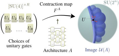
Consider fixing an -gate architecture , then choosing the gates in the architecture. The resulting circuit implements some -qubit unitary. All the unitaries implementable with form a set . Our proof relies on properties of —namely, on the number of degrees of freedom in . We define this number as the architecture’s accessible dimension, (Fig. 3). The following section contains a formal definition; here, we provide intuition. As the -qubit unitaries form a space of dimension , . The greater the , the more space fills in the set of -qubit unitaries. Considering circumvents the intractability of calculating a unitary’s circuit complexity. To better understand the form of , we study the set’s dimension, which is the accessible dimension. Importantly, the accessible dimension enables us to compare the sets generated by different architectures. Distinct accessible dimensions imply that the lower-dimensional set has measure zero in the higher-dimensional set. As a proxy for quantum complexity, the accessible dimension plays a role similar to -designs in Refs. brandao2019models; brandao_efficient_2016. Our first technical result lower-bounds sufficiently connected architecture’s accessible dimension:
Proposition 1 (Lower bound on accessible dimension).
Let denote an architecture formed by concatenating blocks of gates each, each block containing a backwards light cone. The architecture’s accessible dimension is lower-bounded as
| (2) |
We can upper-bound , for an arbitrary architecture , by counting parameters. To synopsize the argument in Appendix B: Fifteen real parameters specify each 2-qubit unitary. Each qubit shared by two unitaries makes 3 parameters redundant. Hence
| (3) |
The accessible dimension reaches its maximal value, , after a number of gates exponential in . Similarly, the circuit complexity reaches its maximal value after exponentially many gates. This parallel suggests as a proxy for the circuit complexity. The next section rigorously justifies the use of as a proxy.
The proof of Theorem 1 revolves around the accessible dimension of a certain -gate architecture . The main idea is as follows. Let be less than a linear fraction of . More specifically, let . For every -gate architecture , holds by a combination of (2) and (3). Consequently, Appendix B in Ref. suppmaterial shows, has zero probability in , according to the measure in Definition 2. Therefore, almost every unitary has a complexity greater than the greatest possible . Inequality (1) follows.
Discussion. We have proven a prominent physics conjecture proposed by Brown and Susskind for random quantum circuits PhysRevD.97.086015; susskind2018black: A local random circuit’s quantum complexity grows linearly in the number of gates until reaching a value exponential in the system size. To prove this conjecture, we introduced a novel technique for bounding complexity. The proof rests on our connecting the quantum complexity to the accessible dimension, the dimension of the set of unitaries implementable with a given architecture (arrangement of gates). Our core technical contribution is a lower bound on the accessible dimension. The bound rests on techniques from differential topology and algebraic geometry.
To the best of our knowledge, Theorem 1 is the first rigorous demonstration of the linear growth of random qubit circuits’ complexities for exponentially long times. The bound holds until the complexity reaches —the scaling, up to polynomial factors, of the greatest complexity achievable by any -qubit unitary NielsenChuang. A hurdle has stymied attempts to prove that local random circuits’ quantum complexity grows linearly: Most physical properties (described with, e.g., local observables or correlation functions) reach fixed values in times subexponential in the system size. One must progress beyond such properties to prove that the complexity grows linearly at superpolynomial times. We overcome this hurdle by identifying the accessible dimension as a proxy for the complexity.
Theorem 1 complements another rigorous insight about complexity growth. In Ref. brandao2019models, the linear growth of complexity is proven in the limit of large local dimension and for a strong notion of quantum circuit complexity, with help from Ref. hunter2019unitary. Furthermore, depth- random qubit circuits have complexities that scale as until brandao2019models; brandao_local_2016. The complexity scales the same way for other types of random unitary evolutions, such as a continuous-time evolution under a stochastically fluctuating Hamiltonian RandomHamiltonians. Finally, Ref. brandao2019models addresses bounds on convergence to unitary designs brandao_local_2016; hunter2019unitary; nakata2017efficient; haferkamp2020quantum; RandomHamiltonians; haferkamp2020improved, translating these bounds into results about circuit complexity. Theorem 1 is neither stronger nor weaker than the results of Ref. brandao2019models, which govern a more operational notion of complexity—how easily can be distinguished from the maximally mixed state.
Our work is particularly relevant to the holographic context surrounding the Brown-Susskind conjecture. There, random quantum circuits are conjectured to serve as proxies for chaotic quantum dynamics generated by local time-independent Hamiltonians PhysRevX.8.021014. Ref. HaydenBlackHoles has introduced this conjecture into black-hole physics, and Ref. susskind2016computational discussed the conjecture in the context of holography. A motivation for invoking random circuits is, random circuits can be analyzed more easily than time-independent–Hamiltonian dynamics. Time-independent–Hamiltonian dynamics are believed to be mimicked also by time-fluctuating Hamiltonians RandomHamiltonians and by random ensembles of Hamiltonians. Furthermore, complexity participates in analogies with thermodynamics, such as a second law of quantum complexity PhysRevD.97.086015. Our techniques can be leveraged to construct an associated resource theory of complexity resourcepaper.
In the context of holography, thermofield double states’ complexities have attracted recent interest susskind2016computational; Eternal; BigComplexity; EntanglementNotEnough. Thermofield double states are pure bipartite quantum states for which each subsystem’s reduced state is thermal. In the context of holography, thermofield double states are dual to eternal black holes in anti-de-Sitter space Eternal. Such a black hole’s geometry consists of two sides connected by a wormhole, or Einstein-Rosen bridge. The wormhole’s volume grows for a time exponential in the number of degrees of freedom of the boundary theory susskind2016computational; PhysRevD.97.086015. As discussed above, random quantum circuits are expected to capture the (presumed Hamiltonian) dynamics behind the horizon. If they do, the growth of the wormhole’s volume is conjectured to match the growth of the boundary state’s complexity susskind2016computational; stanford2014complexity; PhysRevD.97.086015; both are expected to reach a value exponentially large in the number of degrees of freedom. Our results govern the random circuit that serves as a proxy for the dynamics behind the horizon. That random circuit’s complexity, our results show strikingly, indeed grows to exponentially large values. This conclusion reinforces the evidence that quantum circuit complexity is the right quantity with which to resolve the wormhole-growth paradox susskind2016computational.
Outlook. Our main result governs exact circuit complexity. In Ref. (suppmaterial, Cor. 2), we generalize the result to a slightly robust notion of circuit complexity. There, the complexity depends on our tolerance of the error in the implemented unitary. Yet, the error tolerance can be uncontrollably small. The main challenge in extending our results to approximate complexity is, the accessible dimension crudely characterizes the set of unitaries implementable with a given architecture. Consider attempting to enlarge this set to include all the -qubit unitaries that lie close to the set in some norm. The enlarged set’s dimension is . The reason is, the enlargement happens in all directions of . Therefore, our argument does not work as for the exact complexity. Extending our results to approximations therefore offers an opportunity for future work. Approximations may also illuminate random circuits as instruments for identifying quantum advantages neill_blueprint_2017; Supremacy; they would show that a polynomial-size quantum circuit cannot be compressed substantially while achieving a good approximation. These observations motivate an uplifting of the present work to robust notions of quantum circuit complexity (see, e.g., Ref. brandao2019models). A possible uplifting might look as follows. Let denote an -gate architecture, and let denote an -gate architecture. Suppose that the accessible dimensions obey . A unitary implemented with has no chance of occupying the set , which has a smaller dimension than . Consider enlarging to include the unitaries that lie -close, for some . If is sufficiently smooth and well-behaved, we expect the enlarged set’s volume, intersected with , to scale as . Furthermore, suppose that unitaries implemented with are distributed sufficiently evenly in [rather than being concentrated close to ]. All the unitaries in except a small fraction could not lie in . We expect, therefore, that all the unitaries in except a fraction have -approximate complexities greater than .
A related opportunity is a proof that Nielsen’s geometric complexity measure grows linearly under random circuits. Such a proof likely requires a more refined characterization of than its dimension. The quantum complexity in Theorem 1 does not lower-bound Nielsen’s complexity. Hence our main results do not immediately imply a similar bound for Nielsen’s complexity. However, proving the approximate circuit complexity’s linear growth would suffice to lower-bound Nielsen’s complexity, due to known inequalities between Nielsen’s complexity and the circuit complexity [Fig. 1(b)] (e.g., Ref. dowling2008geometry).
We expect our machinery to be applicable to random processes that more closely reflect a variety of systems that are studied in the many-body physics community. Examples include randomly fluctuating dynamics RandomHamiltonians, which implement random quantum circuits when Trotterized, and thermofield-double states undergoing random “shocks” shenker2014black; shenker2014multiple; bouland2019computational. Additionally, hybrid circuits—random unitary circuits punctuated by intermediate measurements—have recently attracted much interest Li_19_Measurement; Skinner_19_Measurement; Chan_19_Unitary, as the amount of entanglement present in such systems appear to undergo phase transitions induced by the rate at which they are measured. A generalization of the accessible dimension to such systems might reveal to what extent circuit complexity, as a measure of entanglement in deep dynamics, undergoes similar phase transitions. We hope that the present work, by innovating machinery for addressing complexity, stimulates further quantitative studies of holography, scrambling, and chaotic quantum dynamics.
Acknowledgements. We thank Aram Harrow and Richard Küng for discussions and thank Péter Varjú for introducing us to the algebraic geometrical methods used in this paper. N. Y. H. thanks Shira Chapman, Michael Walter, and the other organizers of the 2020 Lorentz Center workshop “Complexity: From quantum information to black holes” for inspiration. This work has been funded by the DFG (EI 519/14-1, CRC 183, for which this is an inter-node Berlin-Cologne project, and FOR 2724), by the Einstein Research Foundation, the FQXi, and by an NSF grant for the Institute for Theoretical Atomic, Molecular, and Optical Physics at Harvard University and the Smithsonian Astrophysical Observatory. Administrative support was provided by the MIT CTP.
Author contributions. J. H. developed the basic proof technique. All authors wrote the manuscript and established the results.
Data and code availability statement. No data or code has been generated in this work.
References
- [1] The run-time of the best known algorithms for the -count [26]—deciding whether the optimal gate decomposition of a circuit presented as a sequence of Clifford gates and gates on qubits involves gates—is , with .
- [2] See the Supplementary Material at [Insert URL].
- [3] Consider conjugating an arbitrary -qubit Pauli operator with a uniformly random Clifford operator . The result, , is a uniformly random -qubit Pauli operator [21, 66, 68]. Therefore, for every initial Pauli operator and every final Pauli operator, some Clifford operator maps one to the other.
- [4] S. Aaronson and D. Gottesman. Improved simulation of stabilizer circuits. Phys. Rev. A, 70:052328, 2004.
- [5] F. Arute et al. Quantum supremacy using a programmable superconducting processor. Nature, 574:505–510, 2019.
- [6] J. Bochnak, M. Coste, and M.-F. Roy. Real algebraic geometry, volume 36. Springer Science & Business Media, 2013.
- [7] B. Bolt, T. G. Room, and G. E. Wall. On the Clifford collineation, transform and similarity groups. i. J. Austr. Math. Soc., 2:60–79, 1961.
- [8] B. Bolt, T. G. Room, and G. E. Wall. On the Clifford collineation, transform and similarity groups. II. J. Austr. Math. Soc., 2:80–96, 1961.
- [9] A. Bouland, B. Fefferman, and U. Vazirani. Computational pseudorandomness, the wormhole growth paradox, and constraints on the AdS/CFT duality. arXiv:1910.14646, 2019.
- [10] F. G. S. L. Brandão, A. W. Harrow, and M. Horodecki. Local random quantum circuits are approximate polynomial-designs. Commun. Math. Phys., 346:397–434, 2016.
- [11] F. G. S. L. Brandão, W. Chemissany, N. Hunter-Jones, R. Kueng, and J. Preskill. Models of quantum complexity growth. arXiv:1912.04297, 2019.
- [12] F. G. S. L. Brandao, A. W. Harrow, and M. Horodecki. Efficient quantum pseudorandomness. Phys. Rev. Lett., 116, 2016.
- [13] A. R. Brown, D. A. Roberts, L. Susskind, B. Swingle, and Y. Zhao. Complexity, action, and black holes. Phys. Rev. D, 93:086006, 2016.
- [14] A. R. Brown, D. A. Roberts, L. Susskind, B. Swingle, and Y. Zhao. Holographic complexity equals bulk action? Phys. Rev. Lett., 116:191301, 2016.
- [15] A. R. Brown and L. Susskind. Second law of quantum complexity. Phys. Rev. D, 97:086015, 2018.
- [16] B.Swingle. Unscrambling the physics of out-of-time-order correlators. Nature Phys., 14:988, 2018.
- [17] A. R. Calderbank, E. M. Rains, P. M. Shor, and N. J. A. Sloane. Quantum error correction via codes over gf (4). IEEE Trans. Inf. Th., 44:1369–1387, 1998.
- [18] A. R. Calderbank, E. M. Rains, P. W. Shor, and N. J. A. Sloane. Quantum error correction and orthogonal geometry. Phys. Rev. Lett., 78:405, 1997.
- [19] A. Chan, R. M. Nandkishore, M. Pretko, and G. Smith. Unitary-projective entanglement dynamics. Phys. Rev. B, 99:224307, Jun 2019.
- [20] S. Chapman, J. Eisert, L. Hackl, M. P. Heller, R. Jefferson, H. Marrochio, and R. C. Myers. Complexity and entanglement for thermofield double states. SciPost Phys., 6:034, 2019.
- [21] R. Cleve, D. Leung, L. Liu, and C. Wang. Near-linear constructions of exact unitary 2-designs. Quant. Inf. Comp., 16:0721–0756, 2016.
- [22] C. Dankert, R. Cleve, J. Emerson, and E. Livine. Exact and approximate unitary 2-designs and their application to fidelity estimation. Phys. Rev. A, 80:012304, 2009.
- [23] M. R. Dowling and M. A. Nielsen. The geometry of quantum computation. Quant. Inf. Comp., 8:861–899, 2008.
- [24] J. Eisert. Entangling power and quantum circuit complexity. arXiv:2104.03332, 2021.
- [25] J. Eisert, M. Friesdorf, and C. Gogolin. Quantum many-body systems out of equilibrium. Nature Phys., 11:124–130, 2015.
- [26] D. Gosset, V. Kliuchnikov, M. Mosca, and V. Russo. An algorithm for the -count. Quant. Inf. Comp., 14:1277–1301, 2014.
- [27] D. Gottesman. Stabilizer codes and quantum error correction. quant-ph/9705052, 1997.
- [28] D. Gottesman. Fault-tolerant quantum computation with higher-dimensional systems. Chaos, Sol. Frac., 10:1749–1758, 1999.
- [29] D. Gottesman. The Heisenberg representation of quantum computers. In S. P. Corney, R. Delbourgo, and P. D. Jarvis, editors, Proceedings of the XXII International Colloquium on Group Theoretical Methods in Physics, 1999.
- [30] D. Gross, K. M. R. Audenaert, and J. Eisert. Evenly distributed unitaries: on the structure of unitary designs. J. Math. Phys., 48:052104, 2007.
- [31] J. Haferkamp and N. Hunter-Jones. Improved spectral gaps for random quantum circuits: large local dimensions and all-to-all interactions. arXiv:2012.05259, 2020.
- [32] J. Haferkamp, F. Montealegre-Mora, M. Heinrich, J. Eisert, D. Gross, and I. Roth. Quantum homeopathy works: Efficient unitary designs with a system-size independent number of non-Clifford gates. arXiv:2002.09524, 2020.
- [33] B. Hall. Lie groups, Lie algebras, and representations: an elementary introduction, volume 222. Springer, 2015.
- [34] P. Hayden and J. Preskill. Black holes as mirrors: quantum information in random subsystems. JHEP, 0709:120, 2007.
- [35] N. Hunter-Jones. Unitary designs from statistical mechanics in random quantum circuits. arXiv:1905.12053, 2019.
- [36] E. Knill. Approximation by quantum circuits. quant-ph/9508006, 1995.
- [37] J. M. Lee. Smooth manifolds. In Introduction to smooth manifolds, pages 1–31. Springer, 2013.
- [38] Y. Li, X. Chen, and M. P. A. Fisher. Measurement-driven entanglement transition in hybrid quantum circuits. Phys. Rev. B, 100:134306, 2019.
- [39] J. Maldacena, S. H. Shenker, and D. Stanford. A bound on chaos. JHEP, 1608:106, 2016.
- [40] J. M. Maldacena. Eternal black holes in anti-de sitter. JHEP, 04:021, 2003.
- [41] J. S. Milne. Algebraic groups: the theory of group schemes of finite type over a field, volume 170. Cambridge University Press, 2017.
- [42] A. Nahum, S. Vijay, and J. Haah. Operator spreading in random unitary circuits. Phys. Rev. X, 8:021014, 2018.
- [43] Y. Nakata, C. Hirche, M. Koashi, and A. Winter. Efficient quantum pseudorandomness with nearly time-independent Hamiltonian dynamics. Phys. Rev. X, 7:021006, 2017.
- [44] C. Neill, P. Roushan, K. Kechedzhi, S. Boixo, S. V. Isakov, V. Smelyanskiy, R. Barends, B. Burkett, Y. Chen, and Z. Chen. A blueprint for demonstrating quantum supremacy with superconducting qubits. 2017.
- [45] M. A. Nielsen. A geometric approach to quantum circuit lower bounds. quant-ph/0502070, 2005.
- [46] M. A. Nielsen and I. L. Chuang. Quantum computation and quantum information. Cambridge Series on Information and the Natural Sciences. Cambridge University Press, 2000.
- [47] M. A. Nielsen, M. R. Dowling, M. Gu, and A. C. Doherty. Optimal control, geometry, and quantum computing. Phys. Rev. A, 73:062323, 2006.
- [48] M. A. Nielsen, M. R. Dowling, M. Gu, and A. C. Doherty. Quantum computation as geometry. Science, 311:1133–1135, 2006.
- [49] A -design is a probability distribution, over unitaries, whose first moments equal the Haar measure’s moments [30, 22, 10]. The Haar measure is the unique unitarily invariant probability measure over a compact group.
- [50] Technically, this bound on the dimension does not follow from Lemma 2 as it does for the bound . The reason is, the quotient space is not necessarily semialgebraic. This difficulty can be resolved via Sard’s theorem [57], which asserts, as a special case, that the Hausdorff dimension of a smooth map’s image is bounded by its domain’s dimension. A semialgebraic set’s dimension is the greatest dimension in its stratification and so agrees with the Hausdorff dimension.
- [51] Technically, the sets of few gates form a set of measure 0 in SU. Circuits are not in SU, as explained in Fig. 3. However, we expected the sentence above to be more intuitive with “short circuits” instead of “sets of few gates.”.
- [52] Again, by “short circuits,” we mean, “sets of few gates.” We replaced the latter phrase for ease of expression.
- [53] E. Onorati, O. Buerschaper, M. Kliesch, W. Brown, A. H. Werner, and J. Eisert. Mixing properties of stochastic quantum Hamiltonians. Commun. Math. Phys., 355:905, 2017.
- [54] A. Polkovnikov, K. Sengupta, A. Silva, and M. Vengalattore. Nonequilibrium dynamics of closed interacting quantum systems. Rev. Mod. Phys., 83:863–883, 2011.
- [55] D. Poulin, A. Qarry, R. Somma, and F. Verstraete. Quantum simulation of time-dependent Hamiltonians and the convenient illusion of Hilbert space. Phys. Rev. Lett., 106:170501, 2011.
- [56] D. A. Roberts and B. Yoshida. Chaos and complexity by design. JHEP, 2017:121, 2017.
- [57] A. Sard. Hausdorff measure of critical images on Banach manifolds. Am. J.f Math., 87:158–174, 1965.
- [58] S. H. Shenker and D. Stanford. Black holes and the butterfly effect. JHEP, 2014(3):1–25, 2014.
- [59] S. H. Shenker and D. Stanford. Multiple shocks. JHEP, 2014(12):1–20, 2014.
- [60] B. Skinner, J. Ruhman, and A. Nahum. Measurement-induced phase transitions in the dynamics of entanglement. Phys. Rev. X, 9:031009, Jul 2019.
- [61] D. Stanford and L. Susskind. Complexity and shock wave geometries. Phys. Rev. D, 90:126007, 2014.
- [62] L. Susskind. Entanglement is not enough. 2014. arXiv:1411.0690.
- [63] L. Susskind. Computational complexity and black hole horizons. Fort. Phys., 64:24–43, 2016.
- [64] L. Susskind. Black holes and complexity classes. arXiv:1802.02175, 2018.
- [65] J. Watrous. Semidefinite programs for completely bounded norms. Th. Comp., 5, 2009.
- [66] Z. Webb. The Clifford group forms a unitary 3-design. 2015. arXiv:1510.02769.
- [67] N. Yunger Halpern, N. B. T. Kothakonda, J. Haferkamp, A. Munson, J. Eisert, and P. Faist. Resource theory of quantum uncomplexity. arXiv e-prints, page arXiv:2110.11371, 2021.
- [68] H. Zhu. Multi-qubit Clifford groups are unitary 3-designs. Phys. Rev. A, 96:062336, 2017.
Methods
Having overviewed the proof at a high level, we fill in the key mathematics. Three points need clarifying. First, we must rigorously define the accessible dimension, or the dimension of , which is not a manifold. Second, we must prove Proposition 1. Finally, we must elucidate steps in the proof of Theorem 1. We address these points using the toolbox of algebraic geometry. We associate with every -gate architecture a contraction map . This function maps a list of gates to an -qubit unitary. The unitary results from substituting the gates into the architecture (Fig. 3). The map contracts every edge (qubit) shared by two vertices (gates) in .
The image of is the set of unitaries implementable with the architecture . is a semialgebraic set, consisting of the solutions to a finite set of polynomial equations and inequalities over the real numbers (see Appendix A for a review). That is a semialgebraic set follows from the Tarski-Seidenberg principle, a deep result in semialgebraic geometry (Appendix A). A semialgebraic set’s dimension quantifies the degrees of freedom needed to describe the set locally. More precisely, a semialgebraic set decomposes into manifolds. The greatest dimension of any such manifold equals the semialgebraic set’s dimension. The dimension of is the architecture ’s accessible dimension. More restricted than a semialgebraic set is an algebraic set, which consists of the solutions to a finite set of polynomial equations.
Just as the contraction map’s image will prove useful, so will the map’s rank, defined as follows. Let denote an input into , such that the denote two-qubit gates. The map’s rank at is the rank of a matrix that approximates linearly around (the rank of the map’s Jacobian at ). The rank is low at if perturbing can influence the -qubit unitary only along few directions in .
Crucially, we prove that has the same rank throughout the domain, except on a measure-zero set, where has a lesser rank. The greater, “dominating” rank is the dimension of . To formalize this result, let denote the locus of points at which has a rank of . Let denote the set of points where has a lesser rank. Let denote the maximum rank achieved by at any point . We prove the following lemma in Appendix B, using the dimension theory of real algebraic sets.
Lemma 1 (Low-rank locus).
The low-rank locus is an algebraic set of measure and so is closed (in the Lie-group topology). Equivalently, is an open set of measure . Consequently, .
Lemma 1 guarantees that the contraction map’s rank equals the accessible dimension almost everywhere in .
We now turn to the proof of Proposition 1. The rank of at each point lower-bounds , by definition. Consider an architecture of blocks, each containing a backwards light cone. We identify an at which is lower-bounded by a quantity that grows linearly with (the number of gates in the architecture ). We demonstrate the point’s existence by constructing circuits from Clifford gates.
Consider a choice of unitary gates. Perturbing a amounts to appending an infinitesimal unitary: . The denotes a 2-qubit Hermitian operator, and . can be written as a linear combination of 2-qubit Pauli strings . (An -qubit Pauli string is a tensor product of single-site operators, each of which is a Pauli operator [, , or ] or the identity, . The -qubit Pauli strings form a basis for the space of -qubit Hermitian operators.) Consider perturbing each gate using a combination of all 15 nontrivial 2-qubit Pauli strings [Fig. 4(a)]: , wherein . The perturbation causes a perturbation of the image under . The latter perturbation is, to first order, . This derivative can be expressed as the original circuit with the Pauli string inserted immediately after the gate [Fig. 4(b)].

The rank of at is the number of parameters needed to parameterize a general perturbation of within the image set . To lower-bound the rank of at a point , we need only show that parameters perturb in independent directions. To do so, we express the derivative as
| (1) |
wherein denotes a Hermitian operator [Fig. 4(c)]. results from conjugating , the Pauli string inserted into the circuit after gate , with the later gates. The physical significance of follows from perturbing the gate in the direction by an infinitesimal amount . The image is consequently perturbed, in , in the direction .
We choose for the gates to be Clifford operators. (The Clifford operators are the operators that map the Pauli strings to the Pauli strings, to within a phase, via conjugation. For every Clifford operator and Pauli operator , equals a phase times a Pauli string [18, 17, 27, 7, 8].) As a result, the operators are Pauli strings (up to a phase). Two Pauli strings are linearly independent if and only if they differ. For Clifford circuits, therefore, we can easily verify whether perturbations of cause independent perturbation directions in : We need only show that the resulting operators are distinct.
We apply that fact to prove Proposition 1, using the following observation. Consider any Pauli string and any backwards-light-cone–containing block of any architecture. We can insert Clifford gates into the block such that two operations are equivalent: (i) operating on the input qubits with before the extended block and (ii) operating with the extended block, then with a one-qubit . Figure 4(d) depicts the equivalence, which follows from the structure of backwards light cones. We can iteratively construct a Clifford unitary that reduces the Pauli string’s weight until producing a single-qubit operator. See Appendix B for details.
We now prove Proposition 1 by recursion. Consider an -gate architecture formed from blocks, each containing a backwards light cone and each of gates. Assume that there exists a list of Clifford gates, which can be slotted into , such that has a rank at . Consider appending a backwards-light-cone–containing block to . The resulting architecture corresponds to a contraction map whose rank is , we show.
By assumption, we can perturb such that its image, , is perturbed in independent directions in . These directions can be represented by Pauli operators , wherein , by Eq. (1). Let denote any Pauli operator absent from . We can append to a backwards-light-cone–containing block, forming an architecture of backwards light cones. We design the new block from Clifford gates such that two operations are equivalent: (i) applying to the input qubits before the extended blocks and (ii) applying the extended block, then a single-site . We denote by the list of gates in augmented with the gates in the extended block. Conjugating the with the new block yields operators , for . They represent the directions in which the image is perturbed by the original perturbations of . The are still linearly independent Pauli operators. Also, the and the single-site form an independent set, because is not in . Meanwhile, the single-site is a direction in which the last block’s final gate can be perturbed. The operators , augmented with the single-site , therefore span independent directions along which can be perturbed. Therefore, lower-bounds the rank of .
We apply the above argument recursively, starting from an architecture that contains no gates. The following result emerges: Consider any architecture that consists of backwards-light-cone–containing blocks. At some point , the map has a rank lower-bounded by . Lemma 1 ensures that the same bound applies to .
To conclude the proof of Theorem 1, we address an architecture whose accessible dimension satisfies . Consider sampling a random circuit with the architecture . We must show that the circuit has a zero probability of implementing a unitary in . To prove this claim, we invoke the constant-rank theorem: Consider any map whose rank is constant locally—in any open neighborhood of any point in the domain. In that neighborhood, the map is equivalent to a projector, up to a diffeomorphism. We can apply the constant-rank theorem to the contraction map: has a constant rank throughout , by Lemma 1. Therefore, acts locally as a projector throughout —and so throughout , except on a measure-0 region, by Lemma 1. Consider mapping an image back, through a projector, to a preimage. Suppose that the image forms a subset of dimension lower than the whole range’s dimension. The backward-mapping just adds degrees of freedom to the image. Therefore, the preimage locally has a dimension less than the domain’s dimension. Hence the preimage is of measure 0 in the domain. We use the unitary group’s compactness to elevate this local statement to the global statement in Theorem 1.
Supplementary Material for “Linear growth of quantum circuit complexity”
J. Haferkamp, P. Faist, N. B. T. Kothakonda, J. Eisert and N. Yunger Halpern
Appendix A Algebraic and semialgebraic sets
For convenience, we review elementary aspects of algebraic geometry over the real numbers. We apply these properties in the proof of Theorem 1. Ref. [6] contains a more comprehensive treatment.
Definition 4 (Algebraic set).
A subset is called an algebraic set, or an algebraic variety, if, for a set of polynomials ,
| (1) |
A subset is called an algebraic subset if is an algebraic set. We call a subset a semialgebraic set if, for sets and of polynomials,
| (2) |
A natural topology on algebraic sets is the Zariski topology.
Definition 5 (Zariski topology).
Let denote an algebraic set. The Zariski topology is the unique topology whose closed sets are the algebraic subsets of .
A traditional definition of “dimension” for algebraic sets involves irreducible sets.
Definition 6 (Irreducible set).
Let denote a topological space. is called irreducible if it is not the union of two proper closed subsets.
Definition 7 (Dimension of algebraic sets).
Let be an algebraic set that is irreducible with respect to the Zariski topology. The dimension of is the maximal length of any chain of distinct nonempty irreducible algebraic subsets of .
The relevant algebraic sets in the proof of Theorem 1 are and . Our interest in semialgebraic sets stems from the following principle. In the following, we refer to a function as a polynomial map if its entries are polynomials in the entries of its input.
Theorem 2 (Tarski-Seidenberg principle).
Let be a polynomial map. If is a semialgebraic set, so is .
The Tarski-Seidenberg principle applies to the map that contracts sets of quantum gates. This application is important for us, because it provides a natural notion of dimension for the contraction map’s image.
All semialgebraic sets (and hence all algebraic sets) decompose into smooth manifolds.
Theorem 3 (Stratification of semialgebraic sets).
If is a semialgebraic set, then , wherein each denotes a smooth manifold. If is an algebraic set of dimension in the sense of Definition 7, then .
This does not depend on the decomposition chosen. This independence motivates the following definition:
Definition 8 (Dimension of semialgebraic sets).
Let denote a semialgebraic set, such that , wherein each denotes a manifold. The greatest dimension of any manifold, , is the semialgebraic set’s dimension.
This definition generalizes Definition 7, due to Theorem 3. One more fact about semialgebraic sets’ dimensions will prove useful:
Lemma 2 (Dimension of an image).
Let be a polynomial map. If is a dimension- semialgebraic set, is of dimension .
Appendix B Proof of the main theorem and lemmata
In this appendix, we prove Lemma 1, Lemma 3, and the main theorem. The proofs rely on the topics reviewed in Appendix A, as well as the following notation and concepts. In differential geometry, the rank of at the point is defined as the rank of the derivative . Mapping lists of gates to unitaries, is a complicated object. We can more easily characterize a map from real numbers to real numbers. Related is a map from Hermitian operators to Hermitian operators: An -qubit state evolves under a Hamiltonian represented by a Hermitian operator, which has real parameters. Therefore, for convenience, we shift focus from unitaries to their Hermitian generators. We construct a map whose domain is the algebra that generates SU. The range is the set of -qubit Hermitian operators, . We construct such a map from three steps, depicted by the dashed lines in Fig. 5.
The first step is a chart, a diffeomorphism that maps one manifold to another invertibly. Our chart acts on the algebra that generates . To define the chart, we parameterize an element of the copy of :
| (3) |
wherein . For each point , we define the local exponential chart as , and we define the analogous as . These charts are standard for matrix Lie groups. Both are locally invertible in small neighbourhoods around and , by a standard result in Lie-group theory [33]. The three-part map, represented by the dashed lines in Fig. 5, has the form .
We now characterize the map’s derivative, to characterize the derivative of , to characterize the rank of . Denote by the derivative evaluated where the Hermitian operators are set to zero, such that each chart reduces to the identity operation. The image of is spanned by the operators
| (4) |
These operators have the form
| (5) |
wherein denotes a two-qubit Pauli operator. We apply the setting above to prove the following lemma.
See 1
Proof.
Consider representing an operator (5) as a matrix relative to an arbitrary tensor-product basis. To identify the matrix’s form, we imagine representing the unitaries in as matrices relative to the corresponding tensor-product basis for . Combining the unitary matrices’ elements polynomially yields the matrix elements of (5).
has the same rank as , because and are local charts [37]. Recall that denotes the locus of points, in , where has a rank . Equivalently, by the invertible-matrix theorem, consists of the points where certain minors of —the determinants of certain collections of matrix elements—vanish. The determinants’ vanishing implies a set of equations polynomial in the matrix elements of —and so, by the last paragraph, polynomial in the entries of matrices in . is a real algebraic set, being the set of operators that satisfy the polynomial equations equivalent to and . Thus, by Definition 4, the points of rank form an algebraic subset of .
We can now invoke properties of algebraic subsets, reviewed in Appendix A. First, we prove that is irreducible in the Zariski topology. The Zariski topology of is coarser than the topology inherited from , identified with . As is connected in the finer topology, so is connected in the Zariski topology. This connectedness implies that is irreducible, as is an algebraic group [41, Summary 1.36]. Being irreducible, has a dimension à la Definition 7. If the low-rank locus is not all of , then it is, by Definition 7, a lower-dimensional algebraic subset. Every dimension- algebraic subset decomposes into a collection of submanifolds, each of which has dimension [6, Prop. 9.1.8]. As a proper submanifold has measure , has measure 0. As an algebraic subset, is closed in the Lie-group topology.
Finally, we prove that . In a small open neighborhood of a point , the contraction map’s rank is constant, by Lemma 1. By the constant-rank theorem [37, Thm 5.13], therefore, acts locally as a projector throughout —and so throughout (except on a region of measure 0, by Lemma 1). The projector has a rank, like , of . A rank- projector has an image that is a dimension- manifold. Hence . The other direction, , follows directly from Sard’s theorem [57]. Let denote the set of points where is rank-. As is a smooth map, Sard’s theorem ensures that upper-bounds the Hausdorff dimension of the image . As is a semialgebraic set, it stratifies into manifolds, by Theorem 3. Therefore, the Hausdorff dimension coincides with the semialgebraic set’s dimension. ∎
Lemma 3 (Existence of a high-rank point).
Let denote any nonnegative integer. Consider any architecture formed from -gate, backwards-light-cone–containing blocks. The map has the greatest rank possible, .

Proof.
Without loss of generality, we assume that all blocks have identical architectures. This assumption will simplify the notation below. We can lift the assumption by complicating the notation.
Consider an arbitrary point . For all , the contraction map has a derivative characterized, in the proof of Lemma 1, with local charts and . The number of gates in is . The map has an image spanned by the partial derivatives . Each partial derivative has the form
| (6) |
(Fig. 6). and denote Pauli operators; each acts nontrivially on just one of the two qubits on which acts nontrivially. We implicitly pad operators with identities wherever necessary, such that the operators act on the appropriate Hilbert space.
We aim to lower-bound the greatest possible rank, , of the map . To do so, we construct a point
| (7) |
We will choose for the ’s to be Clifford gates. A gate’s subscript, , labels the blocks to which the gate belongs. The superscript, , labels the gate’s position within the block. The gates constitute a block as . Our construction of relies on a property of an arbitrary Pauli operator : We can choose the Clifford gates such that block maps to a on qubit : . We now show how the existence of such a Clifford unitary implies Lemma 3. Afterward, we show to construct .
Let us choose the Pauli strings that guide our construction of the Clifford block . We choose the ’s inductively over such that is linearly independent. We start with an arbitrary Pauli string . The form of guides our construction of . Second, we choose for to be an arbitrary Pauli string . guides our construction of . Third, we choose for to be an arbitrary Pauli string outside . This guides our construction of . After steps, we have constructed all the ’s and ’s. If , enough Pauli strings exist that, at each step, a Pauli string lies outside the relevant span.
The operators , for , are in the image of :
| (8) | ||||
We have assumed, without loss of generality, that each block’s final gate acts on qubit . For all , the operators are in the image of and are linearly independent. Therefore, the rank of at the point is .
In the remainder of this proof, we provide the missing link: We show that, for every Pauli string , we can construct a backwards-light-cone–containing block that implements a Clifford unitary such that . We drop subscripts because subscripts index blocks and this prescription underlies all blocks. By definition, each block contains a qubit to which each other qubit connects via gates in the block. The path from a given qubit depends on , and multiple paths may connect a to . Also, one path may connect to multiple qubits. We choose an arbitrary complete set of paths (which connect all the other qubits to ) that satisfies the merging property described below. To introduce the merging property, we denote by the number of paths in the set. Let index the paths. Path contacts the qubits in the order , reaching qubits. We choose the paths such that they merge whenever they cross: If , then for all . We choose for all the gates outside these paths to be identities. Next, we choose the nontrivial gates in terms of an arbitrary Pauli string.
Let denote an arbitrary nontrivial -qubit Pauli string. Some Clifford unitary maps to a Pauli string that acts nontrivially on just one qubit (see Refs. [21, 66, 68] and [3]), which we choose to be . We arbitrarily choose for the string’s nontrivial single-qubit Pauli operator to be . Let denote the first index in for which . By definition, is a nontrivial Pauli string. There exists a two-local Clifford gate that transforms into a acting on qubit :
| (9) |
Operating with (padded with ’s) on the whole string yields another Pauli string:
| (10) |
Let denote the first index for which is a nontrivial Pauli operator. Since
| (11) |
. There exists a two-local Clifford gate that shifts the down the path:
| (12) |
We perform this process—of shifting the down the path and leaving an behind—for every path simultaneously. For example, if we begin with two equal-length paths, . This simultaneity is achievable until two paths merge. Whenever paths merge, we choose the next Clifford gate such that we proceed along the merged path. Every qubit is visited, and every path ends at qubit . Therefore, we have constructed a circuit that implements a Clifford operation such that . Figure 4(d) depicts an example of this construction. ∎
The foregoing proof has a surprising implication: A map’s rank is somewhat divorced from a circuit’s complexity. The rank of at is at least , which could be a large number. Yet, the contracted unitary corresponding to this circuit is Clifford. Hence the extended circuit’s complexity surpassed the original circuit’s complexity only a little—by, at most, [4].

See 1
Proof of Theorem 1.
We reuse the notation introduced in Lemmata 1 and 3. Examples include , an arbitrary architecture that satisfies the assumptions in Lemma 3 and that consists of gates. denotes the corresponding contraction map. denotes the locus of points at which achieves its greatest rank, . In a small open neighborhood of a point , the contraction map’s rank is constant, by Lemma 1. By the constant-rank theorem [37, Thm 5.13], therefore, acts locally as a projector throughout —and so throughout (except on a region of measure 0, by Lemma 1). The projector has a rank, like , of . Therefore, in the open set , is equivalent, up to a diffeomorphism, to the projection
| (13) |
For simplicity of notation, we identify with its image under the local diffeomorphism (we do not distinguish from its image notationally).
The open subset contains, itself, an open subset that decomposes as a product: , such that and, as suggested by Eq. (13),
| (14) |
(Again to simplify notation, we are equating the local sets with their images, under local charts, in , for .) From now on, is the open subset of interest. The contraction map’s equivalence to a projector, in , will help us compare high-depth circuits with low-depth circuits: Consider a circuit whose contraction map takes some local neighborhood to an image of some dimension. How does the dimension differ between high-depth circuits and low-depth circuits? We start by upper-bounding the dimension for low-depth circuits.
We have been discussing an -gate architecture . Consider any smaller architecture of gates. is encoded in a contraction map whose domain is . As explained in the proof of Lemma 1, is a polynomial map. Therefore, has a property prescribed by the Tarski-Seidenberg principle [6] (Theorem 2): The image is a semialgebraic set of dimension .
We can strengthen this bound: Consider contracting two gates that share a qubit. The shared qubit may undergo a one-qubit gate specified by three parameters (one parameter per one-qubit Pauli). The one-qubit gate can serve as part of the first two-qubit gate or as part of the second two-qubit gate; which does not affect the contraction. Hence the contraction contains 3 fewer parameters than expected 11 1 In other words, the contraction has a redundant copy of the gauge group SU: Every unitary SU decomposes as , wherein and the and the denote single-qubit unitaries [khaneja2000cartan].. Let us classify the shared qubit as an input of the second two-qubit gate. A two-qubit gate in a circuit’s bulk accepts two input qubits outputted by earlier gates. So we might expect an -gate circuit to have . But the first gates [the leftmost vertical line of gates in Fig. 2(a)] receive their input qubits from no earlier gates. So we must restore parameters for each of the initial gates, or restore parameters total 22 2 Technically, this bound on the dimension does not follow from Lemma 2 as it does for the bound . The reason is, the quotient space is not necessarily semialgebraic. This difficulty can be resolved via Sard’s theorem [57], which asserts, as a special case, that the Hausdorff dimension of a smooth map’s image is bounded by its domain’s dimension. A semialgebraic set’s dimension is the greatest dimension in its stratification and so agrees with the Hausdorff dimension. :
| (15) |
We have upper-bounded the dimension for low-depth circuits.
We now lower-bound the corresponding dimension for high-depth circuits. We can do so by lower-bounding the greatest possible rank, , of a high-depth architecture’s contraction map, : In an open neighborhood of , is equivalent to a projector, which has some rank. The neighborhood’s image, under the projector, is a manifold. The manifold’s dimension equals the projector’s rank. Therefore, we bound the rank to bound the dimension.
Augmenting an architecture with -gate blocks increases the contraction map’s greatest possible rank, , by . Therefore, for an architecture- circuit of gates, we have constructed a point of rank . Therefore,
| (16) |
We have lower-bounded the dimension of the image of a high-depth architecture’s contraction map [the rank in Ineq. (16)] and have upper-bounded the analogous dimension for a low-depth architecture [Ineq. (15)]. The high-depth-architecture dimension upper-bounds the low-depth-architecture dimension,
| (17) |
if
| (18) |
by Ineq. (15). Furthermore, by Ineqs. (15) and (16), Ineq. (17) holds if , or
| (19) |
holds. We have upper-bounded the short circuit’s gate count in terms of the deep circuit’s gate count.
Let us show that, if Ineq. (19) holds, the short circuits form a set of measure 0 in SU 33 3 Technically, the sets of few gates form a set of measure 0 in SU. Circuits are not in SU, as explained in Fig. 3. However, we expected the sentence above to be more intuitive with “short circuits” instead of “sets of few gates.”. We will begin with a point ; apply the short-architecture contraction map ; and follow with the deep-architecture contraction map’s inverse, . The result takes up little space in SU, we will see.
To make this argument rigorous, we recall the small open neighborhood of . In , has the preimage, under , of
| (20) |
The represents our identification of the map with its representation in local charts. By the proof of Lemma 1, is a semialgebraic set. Therefore, by Theorem 3, is a union of smooth manifolds. Each manifold is of dimension , by Theorem 3 and Ineq. (15). By Eq. (14), is of dimension . Therefore, consists of manifolds of dimension . Using Ineq. (18), we can cancel the with the , at the cost of loosening the bound: consists of manifolds of dimension . As a collection of manifolds of submaximal dimension, the unitaries implemented by short circuits satisfying (19), restricted to a small open neighborhood , form a set of measure 44 4 Again, by “short circuits,” we mean, “sets of few gates.” We replaced the latter phrase for ease of expression..
Let us extend this conclusion about -qubit unitaries—about images of maps —to a conclusion about preimages—about lists of gates. By Lemma 1, is of measure . Therefore, for every , there exists a compact subset of measure . Since is compact, for any cover of by open subsets, a finite subcover exists. The foregoing paragraph shows that, restricted to each open set in this finite subcover, the preimage of the unitaries reached by lower-depth circuits is of measure . Therefore, the preimage of the -gate, architecture- circuits is of measure . Since is arbitrary, the preimage is of measure . The foregoing argument holds for each architecture of gates. Hence each preimage forms a set of measure . The total measure is subadditive. So the union of the preimages, over all architectures with gates, is of measure . We have proven the circuit-complexity claim posited in Theorem 1. The state-complexity claim follows from tweaks to the proof (Appendix C). ∎
Appendix C Proof of the linear growth of state complexity
At the end of Appendix B, we proven part of Theorem 1—that circuit complexity grows linearly with the number of gates. Here, we prove rest of the theorem—that state complexity grows linearly. We need only tweak the proof presented in Appendix B.
Consider instead of the contraction map , the map that contracts a list of gates, forming an architecture- circuit, and applies the circuit to , to get
| (21) |
The argument works the same as in Appendix B, with one exception: The derivative has an image that does not contain nontrivial linearly independent Pauli operators. Rather, the image contains the computational basis formed by applying tensor products of and to . (We denote the imaginary number by .) The proof of Lemma 1 ports over without modification, as is a polynomial map between algebraic sets.
The proof of Lemma 3 changes slightly. We must prove the existence of a point at which has a rank at least linear in the circuit depth. The only difference in the proof is, we must choose the operators inductively such that the states are linearly independent. Such a choice is possible if , the number of real parameters in a pure -qubit state vector.
Appendix D Randomized architectures
From Theorem 1 follows a bound on the complexity of a doubly random circuit: Not only the gates, but also the gates’ positions, are drawn randomly. This model features in Ref. [10]. Our proof focuses on nearest-neighbor gates, but other models (such as all-to-all interactions) yield similar results.
Corollary 1 (Randomized architectures).
Consider drawing an -qubit unitary according to the following probability distribution: Choose a qubit uniformly randomly. Apply a Haar-random two-qubit gate to qubits and . Perform this process times. With high probability, the unitary implemented has a high complexity: For all ,
| (22) |
Proof.
The proof relies on the following strategy: We consider constructing blocks randomly to form a circuit. If the blocks contain enough gates, we show, many of the blocks contain backwards light cones. This result enables us to apply Theorem 1 to bound the circuit’s complexity.
Consider drawing gates’ positions uniformly randomly. For each gate, the probability of drawing position is . The probability that no gates act at position is . Let us choose for each block to contain gates. Define a binary random variable as follows: If one of the gates drawn during steps acts at , then . Otherwise, . With high probability, gates act at all positions:
| (23) |
We have invoked the inverse Bernoulli inequality and the Bernoulli inequality. We will use this inequality to characterize blocks that contain backwards light cones.
Consider drawing -gate blocks randomly, as described in the corollary. Denote by the number of blocks in which at least one position is bereft of gates: For some , . With high probability, is small: For all ,
| (24) |
by Markov’s inequality. Let us choose for the threshold to be . With overwhelming probability, blocks satisfy and so contain gates that act at all positions in increasing order. Therefore, these blocks contain a staircase architecture and so contain backwards light cones. Therefore, a slight variation on Theorem 1 governs the gates that form the blocks. Strictly speaking, Theorem 1 governs only consecutive backwards-light-cone–containing blocks. In contrast, extra gates may separate the blocks here. However, the extra gates can only increase the contraction map’s image. Therefore, the additional gates cannot decrease the accessible dimension . Therefore, the bound from Theorem 1 holds. With probability over the choice of architecture,
| (25) |
with probability one over the choice of gates. This bound is equivalent to Ineq. (22). ∎
Appendix E Proof of Corollary 2
Corollary 2 extends Theorem 1 to accommodate errors in the target unitary’s implementation. We prove Corollary 2 by drawing on the proof of Theorem 1 and reusing notation therein.
Corollary 2 (Slightly robust circuit complexity).
Let denote the -qubit unitary implemented by any random quantum circuit in any architecture that satisfies the assumptions in Theorem 1. Let denote the -qubit unitary implemented by any circuit of gates. For every , there exists an such that the Frobenius distance , with probability , unless .
Proof of Corollary 2.
The proof of Theorem 1 can be modified to show that, for every , there exists an open set that contains , such that the preimage is small—of measure . The modification is as follows. For every , there exists a measure- compact subset of . As is compact, there exists a finite cover of that has the following properties: is in the union of subsets . On the , the contraction map is equivalent to a projector, up to a local diffeomorphism. As in the proof of Theorem 1, we can assume, without loss of generality, that . The and are defined analogously to the and in the proof of Theorem 1. For each , there exists an open neighborhood of such that has an arbitrarily small measure . Therefore, has a preimage of measure . Each of the summands, though positive, can be arbitrarily small.
The Frobenius norm induces a metric on . In terms of , we define the function
| (26) |
This function is continuous, and is compact. Therefore, the function achieves its infimum at a point . Therefore, the minimal distance to is . Since is open, is closed and so compact. By the same argument,
| (27) |
We have identified an that satisfies Corollary 2. ∎
Appendix F Notions of circuit complexity
As circuit complexity is a widely popular concept, there is a zoo of quantities that measure it. We prove our main theorem for the straightforward definition of exact circuit implementation—the clearest and historically first notion of a circuit complexity—and for a version of approximate circuit complexity (Corollary 2) with an uncontrollably small error. In this appendix, we briefly mention other notions of complexity, partially to review other notions and partially to place the main text’s findings in a wider context. Let SU denote a unitary. Ref. [48] discusses notions of approximate circuit complexity.
Definition 9 (Approximate circuit complexity).
The approximate circuit complexity is the least number of -local gates, arranged in any architecture, that implements up to an error in operator norm .
This definition is similar in mindset to the above (slightly) robust definition of a circuit complexity. For every pair SU of circuits, the Frobenius distance between them satisfies
| (28) |
A widely used proxy for quantum circuit complexity—one that is increasingly seen as a complexity measure in its own right—is Nielsen’s geometric approach to circuit and state complexity [45, 48, 23]. This approach applies geometric reasoning to circuit complexity and led to many intuitive insights, including Brown and Susskind’s conjectures about the circuit complexity’s behavior under random evolution. To connect to cost functions as considered in Nielsen’s framework, consider -local and -local Hamiltonian terms in the Lie algebra of traceless Hermitian matrices, normalized as for . Consider generating a given unitary, by means of a control system, following Schrödinger’s equation:
| (29) |
The control function is defined as and satisfies . That is, a quantum circuit results from time-dependent control. In practice, not all of reflects meaningful control parameters; merely a control region does. With each parameterized curve is associated a cost function , so that the entire cost of a unitary SU becomes
| (30) |
We take the infimum over all time intervals and over all control functions such that the control parameters are in for all and scuh that . Several cost functions are meaningful and have been discussed in the literature. A common choice is
| (31) |
In particular, gives rise to a sub-Riemannian metric. For the resulting cost , Ref. [47] establishes a connection between the approximate circuit complexity and the cost: Any bound on the approximate circuit complexity, with an approximation error bounded from below independently of the system size, immediately implies a lower bound on the cost.
Theorem 4 (Approximate circuit complexity and cost [47]).
For every integer , every and every ,
| (32) |
The quantity on the right-hand side can, in turn, be upper-bounded: . This has a simple interpretation in terms of a weighted gate complexity [24].
Definition 10 (Weighted circuit complexities).
Let denote a unitary. The weighted circuit complexity equals the sum of the weights of -local gates, arranged in any architecture, that implement , wherein each gate is weighted by its strength , defined through
| (33) |
The weighted circuit complexity turns out to equal the cost for any given unitary. We can grasp this result by Trotter-approximating the time-dependent parameterized curve in the definition of .
Lemma 4 (Weighted circuit complexity and cost).
If denotes an integer and , then
| (34) |
Therefore, the weighted circuit complexity grows like the cost . By implication, the circuit complexity’s growth will be reflected by a notion of circuit complexity that weighs the quantum gates according to their strengths. Again, once the main text’s approximate circuit complexity is established with an -independent approximation error, one finds bounds on the weighted circuit complexity, as well.
The last important notion of circuit complexity that has arisen in the recent literature is that of Ref. [11]. Denote by SU the set of -qubit unitary circuits comprised of elementary quantum gates, wherein the first qubits form the actual system and the next qubits form a memory. Let denote the class of all two-outcome measurements, defined on qubits, that require quantum circuits whose implementation requires elementary quantum gates. Define
| (36) | |||||
In terms of this quantity, Ref. [11] defined strong unitary complexity.
Definition 11 (Strong unitary complexity [11]).
Let and . A unitary SU has strong unitary complexity if
| (37) |
denoted by .
While seemingly technically involved, the definition is operational. The definition is also more stringent and demanding than more-traditional definitions of approximate circuit complexity. To concretize this statement, we denote the diamond norm by [65].
Lemma 5 (Implications of strong unitary complexity [11]).
Suppose that obeys for some , , arbitrary measurement procedures that include the Bell measurement. Then
| (38) |
That is, it is impossible to accurately approximate with circuits of elementary quantum gates.
and denote the unitary quantum channels defined by and . The diamond norm between them is
| (39) | |||||
We have added and subtracted a term and have used the triangle inequality. Therefore,
| (40) |
as the operator norm is a weakly unitarily invariant norm. Therefore, implies that . That is, the strong unitary complexity of Ref. [11] is tighter than approximate circuit complexity. A topic of future work will be the exploration of the growth of approximate notions of complexity with an approximation error independent of the system size.