跳到论文正文
W Papers独立论文阅读器 arXiv:2106.05183 论文正文 计算阅读时间 · 0%
引用这篇论文根据当前论文元数据生成,正式投稿前建议核对。


License: arXiv.org perpetual non-exclusive license
arXiv:2106.05183v1 [math.PR] 09 Jun 2021

Shrinkage Estimation of Functions of Large Noisy Symmetric MatricesThanks: ∗panagd@stanford.eduThanks: †lexing@stanford.eduThanks: 1 Department of Mathematics, Stanford University

Panagiotis Lolas ∗1 and Lexing Ying†1\;{}^{\dagger 1}
Abstract.

We study the problem of estimating functions of a large symmetric matrix AA when we only have access to a noisy estimate A^n=An+σ​Zn/n.\hat{A}_{n}=A_{n}+\sigma Z_{n}/\sqrt{n}. We are interested in the case that ZnZ_{n} is a Wigner ensemble and suggest an algorithm based on nonlinear shrinkage of the eigenvalues of A^n.\hat{A}_{n}. As an intermediate step we explain how recovery of the spectrum of AnA_{n} is possible using only the spectrum of A^n\hat{A}_{n}. Our algorithm has important applications, for example, in solving high-dimensional noisy systems of equations or symmetric matrix denoising. Throughout our analysis we rely on tools from random matrix theory.

1. Introduction

1.1. Problem and Assumptions

Let An∈ℝn×nA_{n}\in\mathbb{R}^{n\times n} be a real symmetric matrix (deterministic or random), which is unknown. Instead, we have access to a noisy estimate A^n=An+σn−1/2Zn.\hat{A}_{n}=A_{n}+\sigma n^{-1/2}Z_{n}. We will often omit the subscript nn in our notation. We will denote by λ1≥λ2≥⋯≥λn\lambda_{1}\geq\lambda_{2}\geq\cdots\geq\lambda_{n} the eigenvalues of An,A_{n}, w1,⋯,wnw_{1},\cdots,w_{n} the corresponding eigenvectors and the empirical spectral distribution of AnA_{n} by μn.\mu_{n}. The latter is the measure μn=n−1​∑k=1nδλk.\mu_{n}=n^{-1}\sum_{k=1}^{n}\delta_{\lambda_{k}}. Similarly we are going to denote by λ^1≥⋯≥λ^n\hat{\lambda}_{1}\geq\cdots\geq\hat{\lambda}_{n} the eigenvalues of A^n\hat{A}_{n} and w^1,⋯,w^n\hat{w}_{1},\cdots,\hat{w}_{n} the corresponding eigenvectors.

Assumptions 1.1.

We assume that AnA_{n} and ZnZ_{n} satisfy the following assumptions.

  1. (1)

    The dimension nn of the matrix AnA_{n} goes to infinity.

  2. (2)

    The spectral distribution of the eigenvalues of AnA_{n} converges weakly almost surely to a deterministic probability measure H.H.

  3. (3)

    The measure HH is supported on a compact interval contained in ℝ\mathbb{R} and eventually all of the eigenvalues of AA lie in a compact subset [h1,h2][h_{1},h_{2}] of ℝ.\mathbb{R}.

  4. (4)

    The matrix ZnZ_{n} is real symmetric and independent of An.A_{n}. The matrix ZnZ_{n} is a submatrix of an infinite matrix (Zi​j)1≤i,j≤n(Z_{ij})_{1\leq i,j\leq n} whose upper half has i.i.d. entries with mean 0, variance 11 and finite fourth moments.

We are interested in estimating h⁡(An),h(A_{n}), where hh is a continuous function defined on an open set that contains [h1,h2][h_{1},h_{2}]. Special cases include, for example, h⁡(x)=xh(x)=x (which is the problem of denoising A^n\hat{A}_{n}), or h⁡(x)=x−1,h(x)=x^{-1}, which is interesting for solving noisy linear systems of equations. Other interesting choices might include h⁡(x)=xh(x)=\sqrt{x} (estimating the square root of a positive semi-definite matrix), or h⁡(x)=x/(x2+λ2)h(x)=x/(x^{2}+\lambda^{2}) (for estimating the regularized inverse of a symmetric matrix).

1.2. Our Contributions

The main contributions of our paper are listed below:

  1. (1)

    We derive (in closed form) the optimal nonlinear shrinkage for estimating h⁡(An)h(A_{n}) in Frobenius loss.

  2. (2)

    We suggest a practical algorithm that asymptotically estimates the optimal nonlinear shrinkage for any choice of function h.h.

  3. (3)

    We study the problem of recovering the limiting spectral distribution HH of the matrix An.A_{n}. We consider the cases of known and unknown noise level σ2.\sigma^{2}. Recovering the measure HH is important for the implementation of our algorithm.

  4. (4)

    We show how our results can be used to derive the optimal shrinkage function with alternative choices of losses.

  5. (5)

    We study asymptotic expansions of the optimal shrinkers when σ→0\sigma\rightarrow 0 and σ→∞.\sigma\rightarrow\infty.

1.3. Related Work

Shrinkage methods have been used in statistics in different settings with great success. In James and Stein 1992 the authors showed how estimation of the mean of a Gaussian distribution in more than 2 dimensions can be improved significantly by shrinkage of the sample estimates. For the purpose of covariance matrix estimation, linear shrinkage methods were used in Ledoit and Wolf 2004 to suggest a well-conditioned estimator of a high-dimensional covariance matrix. Using tools from random matrix theory, in Ledoit et al. 2012 the authors showed how nonlinear shrinkage methods can be used to greatly improve estimation and a nonparametric procedure that achieves greater speed and numerical stability was suggested in Ledoit et al. 2020. For the case of spiked models, Donoho et al. 2018 used nonlinear shrinkage to estimate the population covariance matrix and derived the optimal shrinker for 26 losses, for most of them in closed form. For regularization of linear discriminant analysis, general nonlinear eigenvalue shrinkage was used in Lolas 2020 to improve the classification accuracy when the feature dimensionality is comparable to the number of samples and sharp classification error asymptotics for any shrinkage function were derived.

For the case of a deformed Wigner model as the one we consider here, Donoho and Gavish 2013 showed how eigenvalue shrinkage can be used for symmetric matrix denoising in the case that AA is low-rank. For the problem considered here, h⁡(x)=xh(x)=x was studied by Bun et al. 2016, where the authors derived the optimal nonlinear shrinkage in closed form using replica symmetry. In that case the authors showed that, given σ,\sigma, the optimal shrinker depends on HH only through the Stieltjes transform of the limiting spectral distribution of A^n.\hat{A}_{n}. This phenomenon makes the optimal shrinkage function easy to estimate (for example, with a similar nonparametric procedure as in Ledoit et al. 2020).

The problem of numerical computation of the free-convolution of two probability measures has been studied in Rao and Edelman 2008, Olver and Nadakuditi 2012. The inverse problem, namely spectrum recovery (which we study for the deformed Wigner case in Section 4), has been well-studied for covariance matrices. In El Karoui et al. 2008 a convex optimization approach was used to recover population spectra from samples. In Kong et al. 2017, the authors used a moment method that works even in the sublinear regime where the dimension of the covariance matrix is much larger than the number of samples. Ledoit and Wolf 2015 used an approach that exploits the natural discreteness of population spectra and suggested solving a nonlinear optimization problem which essentially matches the empirical eigenvalues to the quantiles of the Marcenko-Pastur distribution. The idea of natural discreteness of the population spectrum will also be useful for the case of additive free-convolution with a semicircular distribution that we consider here.

Finally, from a Bayesian perspective shrinkage methods have been considered in other settings. In a closely related problem in Etter and Ying 2020 the authors suggested a Bayesian shrinkage method to solve noisy elliptic systems of equations. For the case of covariance matrix estimation, linear shrinkage is motivated by imposing am inverse Wishart prior, while other more sophisticated priors give rise to nonlinear shrinkage methods (Yang and Berger 1994,Berger et al. 2020).

1.4. Organization of the Paper

In Section 2 we review some well-known results from random matrix theory and present a new result about trace functionals that involve both AnA_{n} and A^n.\hat{A}_{n}. These are going to be the essential tools that we will need for the rest of the paper. In Section 3 we derive the oracle nonlinear shrinkage estimators for general continuous functions of AA and asymptotic equivalents that are amenable to estimation. We also suggest an algorithm to perform asymptotically optimal nonlinear shrinkage, when H,σH,\sigma are known. Section 4 considers the problem of recovering H,σ.H,\sigma. Firstly, we show how HH can be recovered, given σ,\sigma, using a nonlinear optimization problem and provide theoretical guarantees for consistency. We then explain how σ\sigma can be consistently estimated for a class of probability measures H.H. In Section 5 we study asymptotic expansions of the shrinkers and the losses when σ→0\sigma\rightarrow 0 and σ→∞.\sigma\rightarrow\infty. Simulations and numerical experiments are presented in Section 6. Finally, Section 7 presents the complete proofs of our results.

2. Almost Sure Limits for a Class of Trace Functionals

In this section we present some useful tools from random matrix theory. We start by introducing our notation and stating well-known theorems. After that, we provide some new results about asymptotics of trace functionals that include both AA and A^\hat{A} which will be essential for justifying the main algorithm in Section 3.

For a probability measure μ\mu supported on the real line we will denote its Stieltjes transform by mμ​(z)=∫(x−z)−1​μ​(𝑑x),z∈ℂ+.m_{\mu}(z)=\int(x-z)^{-1}\mu(dx),z\in\mathbb{C}^{+}. We will often omit the measure from the subscript and just write m⁡(z),m(z), provided that it is clear which measure we are referring to. We have the following well-known result, the so-called Wigner semicircle law (Wigner 1958).

Theorem 2.1 (Theorem 2.4.2 in Tao 2012).

Let (Mi​j)1≤i,j\left(M_{ij}\right)_{1\leq i,j} be mean 0, variance 1 real random variables such that Mi​j=Mj​iM_{ij}=M_{ji} and (Mi​j)i<j\left(M_{ij}\right)_{i<j} are independent and identically distributed. Then, the spectral distribution of the sequence of random matrices n−1/2Mn=(n−1/2Mi​j)1≤i,j≤nn^{-1/2}M_{n}=\left(n^{-1/2}M_{ij}\right)_{1\leq i,j\leq n} converges weakly almost surely to the Wigner semicircular distribution:

μs​c=(4−x2)+2​π​d​x.\mu_{sc}=\frac{\sqrt{(4-x^{2})_{+}}}{2\pi}dx.

The above result gives the limiting spectral distribution of Wigner matrices. For the case of a deformed Wigner matrix, such as A^n=An+σn−1/2Zn,\hat{A}_{n}=A_{n}+\sigma n^{-1/2}Z_{n}, we have under the Assumptions 1.1 in Subsection 1.1:

Proposition 2.1.

The matrix A^n\hat{A}_{n} has a limiting spectral distribution μ^\hat{\mu}, which is a deterministic probability measure with Stieltjes transform mμ^​(z)m_{\hat{\mu}}(z) that satisfies:

mμ^​(z)=∫d​H​(t)t−z−σ2​mμ^​(z).m_{\hat{\mu}}(z)=\int\frac{dH(t)}{t-z-\sigma^{2}m_{\hat{\mu}}(z)}.

This is the formula that describes the free additive convolution H⊞ρs​c;σ2H\boxplus\rho_{sc;\sigma^{2}} of a measure with a semicircular distribution (Biane 1997). If H=δ0,H=\delta_{0}, we can solve for the Stieltjes transform mμ^​(z)m_{\hat{\mu}}(z) in closed form and then use Stieltjes inversion to recover the Wigner law.

The first main contribution of this paper is to extend this result in the following theorem, which is analogous to the results in Ledoit and Péché 2011 for the case of covariance matrices. As in the case of covariance matrices, when Ledoit et al. 2012 used it to estimate a covariance matrix using nonlinear shrinkage, this is going to be the main tool for theoretically justifying our algorithms. In Bun et al. 2016 a similar calculation is done using using replica symmetry for matrices corrupted by orthogonally invariant noise.

Theorem 2.2.

With the same assumptions as in Section 1 we have for any z∈ℂ+z\in\mathbb{C}^{+}

t​r​(h⁡(A)​(A^−z)−1)n→a.s.∫h⁡(t)​d​H​(t)t−z−σ2​mμ^​(z).\frac{tr\left(h(A)\left(\hat{A}-z\right)^{-1}\right)}{n}\xrightarrow{a.s.}\int\frac{h(t)dH(t)}{t-z-\sigma^{2}m_{\hat{\mu}}(z)}.

Here, mμ^​(z)m_{\hat{\mu}}(z) is the Stieltjes transform of the free additive convolution of HH with a semicircular distribution of variance σ2,\sigma^{2}, as in Proposition 2.1.

Although the theorem above was stated for a function hh that is continuous, it can be extended to cases with finitely many discontinuities which are not on atoms of the measure H.H. In that case, taking h⁡(t)=𝕀[a,b]h(t)=\mathbb{I}_{[a,b]} gives the asymptotic overlap of the eigenvectors of A,A^,A,\hat{A}, which the authors in Bun et al. 2016 derived.

3. Main Results

In this section, we motivate and present the main algorithm of the paper. We start by deriving an oracle estimator that optimally approximates h⁡(A)h(A) among all rotationally invariant estimators. We also find the optimal shrinker in closed form using the results from Section 2. After that, we explain how universality, namely the fact that in the large nn limit the distribution of the noise does not affect the asymptotics we are interested in, can be used to simulate approximately the optimally shrunk eigenvalues.

3.1. Optimal Rotation Invariant Estimator

We consider the spectral decomposition of A^,\hat{A}, which has eigenvalues λ^1≥⋯≥λ^n:\hat{\lambda}_{1}\geq\cdots\geq\hat{\lambda}_{n}:

A^=W^​Λ^​W^⊺.\hat{A}=\hat{W}\hat{\Lambda}\hat{W}^{\intercal}.

For a continuous function hh, an estimator Ψ⁡(A^)\Psi(\hat{A}) of h⁡(A)h(A) is rotationally invariant if Ψ⁡(O​A^​O⊺)=O​Ψ​(A^)​O⊺\Psi(O\hat{A}O^{\intercal})=O\Psi(\hat{A})O^{\intercal} for any n×nn\times n orthogonal matrix O.O. Searching for a rotationally invariant estimator of h⁡(A)h(A) seems reasonable, if we do not have any prior information about the eigenstructure of A.A. If such information was available, we might be able to exploit it by approaching the problem in a Bayesian way. With that in mind, it also seems reasonable to consider Ψ⁡(A^)\Psi(\hat{A}) with the same eigenvectors as A^,\hat{A}, such that Ψ⁡(A^)=W^​D​W^⊺.\Psi(\hat{A})=\hat{W}{D}\hat{W}^{\intercal}. We are interested in choosing Ψ\Psi to minimize the Frobenius loss ‖Ψ⁡(A^)−h⁡(A)‖F2.\left\lVert\Psi(\hat{A})-h(A)\right\rVert_{F}^{2}. We observe that

‖Ψ⁡(A^)−h⁡(A)‖F2=‖D−W^⊺​h​(A)​W^‖F2,\left\lVert\Psi(\hat{A})-h(A)\right\rVert_{F}^{2}=\left\lVert D-\hat{W}^{\intercal}h(A)\hat{W}\right\rVert_{F}^{2},

which is minimized when

D(h)=(d1(h),⋯,dn(h))=diag⁡(W^⊺​h​(A)​W^).D^{(h)}=(d_{1}^{(h)},\cdots,d_{n}^{(h)})=\operatorname{diag}(\hat{W}^{\intercal}h(A)\hat{W}). (1)

These clearly depends on the unknown matrix AA and is not straightforward to estimate from the data. In the case h⁡(x)=xh(x)=x the authors in Bun et al. 2016, Potters and Bouchaud 2020 show that the oracle quantities can be asymptotically approximated by deterministic quantities that depend only on the limiting spectral distribution of A^\hat{A} and the noise σ.\sigma. The authors call this remarkable phenomenon the large dimension miracle. It makes the oracle quantities amenable to estimation, for example via kernel estimation. However, such a miracle does not seem very likely in the case of a general hh (and it is not entirely clear how to extend to the case of unknown σ\sigma). For example, already for h⁡(x)=x−1,h(x)=x^{-1}, we will see that the optimal shrinkage is given by

f1/t∗​(x)≡x+σ2​∫t−1​𝑑H​(t)(x+σ2​u​(x))2+σ4​v​(x)2,f_{1/t}^{*}(x)\equiv\frac{x+\sigma^{2}\int t^{-1}dH(t)}{(x+\sigma^{2}u(x))^{2}+\sigma^{4}v(x)^{2}},

where u⁡(x)u(x) and v⁡(x)v(x) are the real and imaginary parts of limη→0+mμ^​(x+i​η)\lim_{\eta\rightarrow 0^{+}}m_{\hat{\mu}}({x+i\eta}), i.e., u⁡(x)+i​v​(x)=limη→0+mμ^​(x+i​η)u(x)+iv(x)=\lim_{\eta\rightarrow 0^{+}}m_{\hat{\mu}}({x+i\eta}). This already requires estimating mH​(0)=∫t−1​𝑑H​(t)m_{H}(0)=\int t^{-1}dH(t) and it is not hard to see that for other functions the situation can get even more complicated.

Definition 3.1.

For a continuous function hh on an open interval that contains the support of H,{H}, we define the functions uh,vh:ℝ→ℝu_{h},v_{h}:\mathbb{R}\rightarrow\mathbb{R} by

uh​(x)+i​vh​(x)=limη↓0∫h⁡(t)​d​H​(t)t−x−i​η−σ2​mμ^​(x+i​η).u_{h}(x)+iv_{h}(x)=\lim_{\eta\downarrow 0}\int\frac{h(t)dH(t)}{t-x-i\eta-\sigma^{2}m_{\hat{\mu}}(x+i\eta)}.
Remark 3.1.

The limit above exists because limη↓0mμ^​(x+i​η)\lim_{\eta\downarrow 0}m_{\hat{\mu}}(x+i\eta) exists (Biane 1997).

Below derive the optimal shrinker for a general continuous function h.h.

Theorem 3.1.

Among all bounded continuous functions ff on an open interval containing s​u​p​p​(H⊞ρs​c;σ2)supp(H\boxplus\rho_{sc;\sigma^{2}}) and the eigenvalues of A^n,\hat{A}_{n}, the minimizer fh∗​(x)f_{h}^{*}(x) of the asymptotic quantity

limn→∞n−1​‖f⁡(A^n)−h⁡(An)‖F2\lim_{n\rightarrow\infty}n^{-1}\left\lVert f(\hat{A}_{n})-h(A_{n})\right\rVert_{F}^{2}

is given by fh∗​(x)=vh​(x)/v⁡(x)f_{h}^{*}(x)=v_{h}(x)/v(x) for x∈s​u​p​p​(H⊞ρs​c;σ2).x\in supp(H\boxplus\rho_{sc;\sigma^{2}}).

According to Theorem 2.2, the measure n−1​∑i=1ndi(h)​δλ^in^{-1}\sum_{i=1}^{n}d_{i}^{(h)}\delta_{\hat{\lambda}_{i}} converges weakly almost surely to a measure with density π−1​vh.\pi^{-1}v_{h}. This suggests that the asymptotic analog of the oracle quantities di(h)d_{i}^{(h)} is the quantity vh/vv_{h}/v derived above. As an immediate corollary of Theorem 3.1 we have the following:

Corollary 3.1.
  1. (1)

    For the choice h⁡(t)=th(t)=t,

    ut​(x)+i​vt​(x)=limz=x+i​η,η↓01+z​mμ^​(z)+σ2​mμ^​(z)2.u_{t}(x)+iv_{t}(x)=\lim_{z=x+i\eta,\eta\downarrow 0}1+zm_{\hat{\mu}}(z)+\sigma^{2}m_{\hat{\mu}}(z)^{2}. (2)

    This gives the optimal shrinkage function ft∗​(x)=x+2​σ2​u​(x)f^{*}_{t}(x)=x+2\sigma^{2}u(x).

  2. (2)

    For the choice h⁡(t)=1/th(t)=1/t,

    u1/t​(x)+i​v1/t​(x)=limz=x+i​η,η↓0mμ^​(z)−mH​(0)z+σ2​mμ^​(z).u_{1/t}(x)+iv_{1/t}(x)=\lim_{z=x+i\eta,\eta\downarrow 0}\frac{m_{\hat{\mu}}(z)-m_{H}(0)}{z+\sigma^{2}m_{\hat{\mu}}(z)}. (3)

    This gives the optimal shrinkage function

    f1/t∗​(x)=x+σ2​mH​(0)(x+σ2​u)2+σ4​v​(x)2.f^{*}_{1/t}(x)=\frac{x+\sigma^{2}m_{H}(0)}{(x+\sigma^{2}u)^{2}+\sigma^{4}v(x)^{2}}.
  3. (3)

    For the choice h⁡(t)=t2h(t)=t^{2},

    ut2​(x)+i​vt2​(x)=limz=x+i​η,η↓0∫t2​d​H​(t)t−z−σ2​mμ^​(z)=limz=x+i​η,η↓0∫t​dH​(t)+z+σ2​mμ^​(z)+mμ^​(z)​[z+σ2​mμ^​(z)]2=∫t​dH​(t)+x+σ2​(u⁡(x)+i​v​(x))+(u⁡(x)+i​v​(x))​[x+σ2​(u⁡(x)+i​v​(x))]2.\begin{split}&u_{t^{2}}(x)+iv_{t^{2}}(x)=\lim_{z=x+i\eta,\eta\downarrow 0}\int\frac{t^{2}dH(t)}{t-z-\sigma^{2}m_{\hat{\mu}}(z)}\\ &=\lim_{z=x+i\eta,\eta\downarrow 0}\int tdH(t)+z+\sigma^{2}m_{\hat{\mu}}(z)+m_{\hat{\mu}}(z)\left[z+\sigma^{2}m_{\hat{\mu}}(z)\right]^{2}\\ &=\int tdH(t)+x+\sigma^{2}(u(x)+iv(x))+(u(x)+iv(x))\left[x+\sigma^{2}(u(x)+iv(x))\right]^{2}.\end{split} (4)

    This gives the optimal shrinkage function

    ft2∗​(x)=σ2+(x+σ2​u​(x))2−σ4​v2​(x)+2​σ2​u​(x)​(x+σ2​u​(x)).f^{*}_{t^{2}}(x)=\sigma^{2}+(x+\sigma^{2}u(x))^{2}-\sigma^{4}v^{2}(x)+2\sigma^{2}u(x)(x+\sigma^{2}u(x)).
Remark 3.2.

Using Theorem 3.1 we can show that for estimating AnkA_{n}^{k} in Frobenius norm we need the first (k−2)(k-2) moments of the measure HH for k≥3.k\geq 3.

3.1.1. Pseudoinverses and Regularized Pseudoinverses

We study the optimal shrinkage to estimate A​(A2+λ2​In)−1.A\left(A^{2}+\lambda^{2}I_{n}\right)^{-1}. If λ↓0,\lambda\downarrow 0, this converges to the pseudoinverse of the matrix A.A. Using our usual notation we have h=h⁡(t,λ)=t/(t2+λ2).h=h(t;\lambda)=t/(t^{2}+\lambda^{2}). This gives

∫h⁡(t)​d​H​(t)t−z−σ2​mμ^​(z)=∫t​d​H​(t)(t2+λ2)​(t−z−σ2​mμ^​(z))=∫[z+σ2​mμ^​(z)(z+σ2​mμ^​(z))2+λ2​1t−z−σ2​mμ^​(z)]​dH​(t)+12​(λ​i−z−σ2​mμ^​(z))∫d​H​(t)t−λ​i−12​(λ​i+z+σ2​mμ^​(z))∫d​H​(t)t+λ​i=mμ^​(z)​(z+σ2​mμ^​(z))(z+σ2​m​(z))2+λ2+mH​(λ​i)2​(λ​i−z−σ2​mμ^​(z))−mH​(−λ​i)2​(λ​i+z+σ2​mμ^​(z))\begin{split}&\int\frac{h(t)dH(t)}{t-z-\sigma^{2}m_{\hat{\mu}}(z)}=\int\frac{tdH(t)}{(t^{2}+\lambda^{2})(t-z-\sigma^{2}m_{\hat{\mu}}(z))}\\ &=\int\left[\frac{z+\sigma^{2}m_{\hat{\mu}}(z)}{(z+\sigma^{2}m_{\hat{\mu}}(z))^{2}+\lambda^{2}}\frac{1}{t-z-\sigma^{2}m_{\hat{\mu}}(z)}\right]dH(t)\\ &+\frac{1}{2(\lambda i-z-\sigma^{2}m_{\hat{\mu}}(z))}\int\frac{dH(t)}{t-\lambda i}-\frac{1}{2(\lambda i+z+\sigma^{2}m_{\hat{\mu}}(z))}\int\frac{dH(t)}{t+\lambda i}\\ &=\frac{m_{\hat{\mu}}(z)(z+\sigma^{2}m_{\hat{\mu}}(z))}{(z+\sigma^{2}m(z))^{2}+\lambda^{2}}+\frac{m_{H}(\lambda i)}{2(\lambda i-z-\sigma^{2}m_{\hat{\mu}}(z))}-\frac{m_{H}(-\lambda i)}{2(\lambda i+z+\sigma^{2}m_{\hat{\mu}}(z))}\end{split} (5)

which allows us to compute the optimal shrinkage as a function of u,v,mH​(λ​i).u,v,m_{H}(\lambda i).

For the case of the pseudoinverse of a Hermitian matrix A,A, we examine the following scenario. We assume that there exist fixed δ>0,p∈(0,1)\delta>0,p\in(0,1) such that AA has ana_{n} eigenvalues equal to 0, n−ann-a_{n} eigenvalues greater than δ\delta and an/n→a.s.pa_{n}/n\xrightarrow{a.s.}{p} as n→∞.n\rightarrow\infty. In that case we can write H=p​δ0+(1−p)​ν,H=p\delta_{0}+(1-p)\nu, where ν\nu is a probability measure with support contained in [δ,∞).[\delta,\infty). Under these assumptions the pseudoinverse of AA can be written as a function h⁡(A),h(A), where hh is continuous on [0,∞],[0,\infty], h⁡(x)=1/xh(x)=1/x for x≥δx\geq\delta and h⁡(x)=0h(x)=0 in an open set containing 00. We find in this case the Stieljes transform of H⊞ρs​c;σ2H\boxplus\rho_{sc;\sigma^{2}} satisfies

mμ^​(z)=−pz+σ2​mμ^​(z)+(1−p)​∫d​ν​(t)t−z−σ2​mμ^​(z).m_{\hat{\mu}}(z)=-\frac{p}{z+\sigma^{2}m_{\hat{\mu}}(z)}+(1-p)\int\frac{d\nu(t)}{t-z-\sigma^{2}m_{\hat{\mu}}(z)}. (6)

Using this we see that

∫h⁡(t)​d​H​(t)t−z−σ2​mμ^​(z)=(1−p)​∫d​ν​(t)t⁡(t−z−σ2​mμ^​(z))=1−pz+σ2​mμ^​(z)​∫[1t−z−σ2​mμ^​(z)−1t]​dν​(t)=1−pz+σ2​mμ^​(z)​[mμ^​(z)+pz+σ2​mμ^​(z)1−p−mν​(0)]=mμ^​(z)z+σ2​mμ^​(z)+p(z+σ2​mμ^​(z))2−(1−p)​mν​(0)z+σ2​mμ^​(z).\begin{split}&\int\frac{h(t)dH(t)}{t-z-\sigma^{2}m_{\hat{\mu}}(z)}\\ &=(1-p)\int\frac{d\nu(t)}{t(t-z-\sigma^{2}m_{\hat{\mu}}(z))}=\frac{1-p}{z+\sigma^{2}m_{\hat{\mu}}(z)}\int\left[\frac{1}{t-z-\sigma^{2}m_{\hat{\mu}}(z)}-\frac{1}{t}\right]d\nu(t)\\ &=\frac{1-p}{z+\sigma^{2}m_{\hat{\mu}}(z)}\left[\frac{m_{\hat{\mu}}(z)+\frac{p}{z+\sigma^{2}m_{\hat{\mu}}(z)}}{1-p}-m_{\nu}(0)\right]\\ &=\frac{m_{\hat{\mu}}(z)}{z+\sigma^{2}m_{\hat{\mu}}(z)}+\frac{p}{(z+\sigma^{2}m_{\hat{\mu}}(z))^{2}}-\frac{(1-p)m_{\nu}(0)}{z+\sigma^{2}m_{\hat{\mu}}(z)}.\end{split} (7)
Remark 3.3.
  1. (1)

    If p=0,p=0, the last formula reduces to

    mμ^​(z)−mν​(0)z+σ2​mμ^​(z)=mμ^​(z)−mH​(0)z+σ2​mμ^​(z).\frac{m_{\hat{\mu}}(z)-m_{\nu}(0)}{z+\sigma^{2}m_{\hat{\mu}}(z)}=\frac{m_{\hat{\mu}}(z)-m_{H}(0)}{z+\sigma^{2}m_{\hat{\mu}}(z)}.

    This, as expected, agrees with Corollay 3.1.

  2. (2)

    When H=p​δ0+(1−p)​ν,H=p\delta_{0}+(1-p)\nu, we have

    mH​(λ​i)=−pλ​i+(1−p)​mν​(λ​i)m_{H}(\lambda i)=-\frac{p}{\lambda i}+(1-p)m_{\nu}(\lambda i)

    and

    mH​(−λ​i)=pλ​i+(1−p)​mν​(−λ​i).m_{H}(-\lambda i)=\frac{p}{\lambda i}+(1-p)m_{\nu}(-\lambda i).

    Using these it is straightforward to see that the optimal shrinkage for the regularized pseudoinverse converges to the optimal shrinkage for the pseudoinverse as λ↓0.\lambda\downarrow 0.

3.2. Monte-Carlo Nonlinear Shrinkage

We are now going to present an algorithm to approximate the oracle quantities. Based on Theorem 3.1, it is natural to try to compute HH and then solve for uh,vhu_{h},v_{h}. Our algorithm does not require solving numerically the equation for the Stieltjes transform of the additive free convolution of HH with a semicircular distribution, which can be tricky (Olver and Nadakuditi 2012). We think that the general idea behind it is likely to be applied in more complicated cases, in particular in problems that do not have simple formulas for the optimal shrinkage as derived in Theorem 3.1. The key observation is that the asymptotic equivalents of the oracle quantities only depend on HH and are universal for all noise distributions. Hence, although A,ZA,Z are unknown, it is possible to replicate the asymptotic equivalents to the oracles using a Monte-Carlo simulation.

Suppose that we know σ,λ1,⋯,λn,\sigma,\lambda_{1},\cdots,\lambda_{n}, or estimates σ~,λ~1,⋯,λ~n\tilde{\sigma},\tilde{\lambda}_{1},\cdots,\tilde{\lambda}_{n} of those are available. The topic of finding suitable choices for σ~\tilde{\sigma} and λ~i\tilde{\lambda}_{i} for 1≤i≤n1\leq i\leq n is going to be the topic of the next section, as suggested by Theorem 4.1. Then, we suggest the following simple procedure in Algorithm 3.1 for approximately optimal nonlinear shrinkage of the eigenvalues of A^\hat{A} to estimate h⁡(A)h({A}) in Frobenius norm. The complexity of the algorithm is 𝒪⁡(K​n3).\mathcal{O}(Kn^{3}). Notice that we use the notation G​O​E​(n)GOE(n) for the Gaussian Orthogonal Ensemble in ℝn×n\mathbb{R}^{n\times n} (Tao 2012).

Algorithm 3.1 MC Nonlinear Shrinkage
1: Inputs: σ~,λ~1,⋯,λ~n\tilde{\sigma},\tilde{\lambda}_{1},\cdots,\tilde{\lambda}_{n} and a positive integer K.K.
2: for k=1,⋯,Kk=1,\cdots,K do
3:   Generate Z^k∼σ~n−1/2GOE(n).\hat{Z}_{k}\sim\tilde{\sigma}n^{-1/2}GOE(n).
4:   Find the eigenvectors g^1,k,⋯,g^n,k\hat{g}_{1,k},\cdots,\hat{g}_{n,k} of d​i​a​g​(λ~1,⋯,λ~n)+Z^kdiag(\tilde{\lambda}_{1},\cdots,\tilde{\lambda}_{n})+\hat{Z}_{k} such that g^i,k\hat{g}_{i,k} corresponds to the i−i-th largest eigenvalue.
5:   Set d^i,k=g^i,k⊺​d​i​a​g​(h⁡(λ~1),⋯,h⁡(λ~n))​g^i,k.\hat{d}_{i,k}=\hat{g}_{i,k}^{\intercal}diag(h(\tilde{\lambda}_{1}),\cdots,h(\tilde{\lambda}_{n}))\hat{g}_{i,k}.
6: Output: di∗=K−1​∑k=1Kd^i,k,1≤i≤n.d_{i}^{*}=K^{-1}\sum_{k=1}^{K}\hat{d}_{i,k},1\leq i\leq n.

Algorithm 3.1 approximates the oracle nonlinear shrinkage in the following sense.

Theorem 3.2.

For a bounded continuous function hh defined on an open set that contains the support of H,H, let di(h)d_{i}^{(h)} be the oracle quantities defined in (1) Subsection 3.1 and di∗d_{i}^{*} the output of the MC Nonlinear Shrinkage algorithm with input σ~,λ~1,⋯,λ~n,K≥1.\tilde{\sigma},\tilde{\lambda}_{1},\cdots,\tilde{\lambda}_{n},K\geq 1. Assume that σ~→σ\tilde{\sigma}\rightarrow\sigma and n−1​∑i=1nδλ~i→a.s.Hn^{-1}\sum_{i=1}^{n}\delta_{\tilde{\lambda}_{i}}\xrightarrow{a.s.}H. Then, for any a,b∈[0,1]:a,b\in[0,1]:

∑[n​a][n​b]di(h)n−∑[n​a][n​b]di∗n→a.s.0.\frac{\sum_{[na]}^{[nb]}d_{i}^{(h)}}{n}-\frac{\sum_{[na]}^{[nb]}d_{i}^{*}}{n}\xrightarrow{a.s.}{0}.

3.3. Different Loss Functions

So far we have been interested in the case of Frobenius loss. For some applications other losses might be more suitable. For this reason we shortly present how our results can be used to derive the optimal nonlinear shrinkage for some other choices of losses. Some of the losses we consider here (and many others) were studied for spiked covariance models in Donoho et al. 2018. Below we will be interested in the following losses:

  1. (1)

    Stein loss: Ls​t(A,B)=tr(A−1B−I)−logdetA−1B.L^{st}(A,B)=tr(A^{-1}B-I)-\log{\det{A^{-1}B}}.

  2. (2)

    Divergence Loss: Ld​i​v​(A,B)=t​r​(A−1​B−I)+t​r​(B−1​A−I).L^{div}(A,B)=tr(A^{-1}B-I)+tr(B^{-1}A-I).

  3. (3)

    The loss L⁡(A,B)=‖A−1​B−I‖F2.L(A,B)=\left\lVert A^{-1}B-I\right\rVert_{F}^{2}.

Proposition 3.1.

Assume that (using the notation from the Assumptions in Section 1) h1>0.h_{1}>0. For any positive and bounded continuous function ff defined on an open set that eventually contains the eigenvalues of A^\hat{A} we have almost surely:

  1. (1)

    For the Stein loss Ls​t​(A,f​(A^))L^{st}(A,f(\hat{A})) we have:

    limn→∞n−1​Ls​t​(A,f⁡(A^))=∫f⁡(x)​v1/t​(x)π​𝑑x+∫log⁡t​𝑑H​(t)−∫log⁡f⁡(x)​v⁡(x)π​𝑑x.\lim_{n\rightarrow\infty}n^{-1}L^{st}(A,f(\hat{A}))=\int f(x)\frac{v_{1/t}(x)}{\pi}dx+\int\log tdH(t)-\int\log{f(x)}\frac{v(x)}{\pi}dx.

    This is minimized for f⁡(x)=v⁡(x)/v1/t​(x)=1/f1/t∗​(x).f(x)=v(x)/v_{1/t}(x)=1/f_{1/t}^{*}(x).

  2. (2)

    For the Stein loss Ls​t​(f​(A^),A)L^{st}(f(\hat{A}),A) we have:

    limn→∞n−1​Ls​t​(f⁡(A^),A)=∫1f⁡(x)​vt​(x)π​𝑑x+∫log⁡f⁡(x)​v⁡(x)π​𝑑x−∫log⁡t​𝑑H​(t)−1.\lim_{n\rightarrow\infty}n^{-1}L^{st}(f(\hat{A}),A)=\int\frac{1}{f(x)}\frac{v_{t}(x)}{\pi}dx+\int\log f(x)\frac{v(x)}{\pi}dx-\int\log tdH(t)-1.

    This is minimized for f⁡(x)=vt​(x)/v⁡(x)=ft∗​(x).f(x)=v_{t}(x)/v(x)=f_{t}^{*}(x).

  3. (3)

    For the divergence loss Ld​i​v​(A,f​(A^))L^{div}(A,f(\hat{A})) we have:

    limn→∞n−1​Ld​i​v​(A,f⁡(A^))=∫f⁡(x)​v1/t​(x)π​𝑑x+∫1f⁡(x)​vt​(x)π​𝑑x−2.\lim_{n\rightarrow\infty}n^{-1}L^{div}(A,f(\hat{A}))=\int f(x)\frac{v_{1/t}(x)}{\pi}dx+\int\frac{1}{f(x)}\frac{v_{t}(x)}{\pi}dx-2.

    This is minimized for f⁡(x)=vt​(x)/v1/t​(x)=ft∗​(x)/f1/t∗​(x).f(x)=\sqrt{v_{t}(x)/v_{1/t}(x)}=\sqrt{f_{t}^{*}(x)/f_{1/t}^{*}(x)}.

  4. (4)

    For the loss L⁡(A,f⁡(A^))L(A,f(\hat{A})) we have:

    limn→∞n−1​L​(A,f⁡(A^))=1−2​∫f⁡(x)​v1/t​(x)π​𝑑x+∫f2​(x)​v1/t2​(x)π​𝑑x.\lim_{n\rightarrow\infty}n^{-1}L(A,f(\hat{A}))=1-2\int f(x)\frac{v_{1/t}(x)}{\pi}dx+\int f^{2}(x)\frac{v_{1/t^{2}}(x)}{\pi}dx.

    This is minimized for f⁡(x)=v1/t​(x)/v1/t2​(x)=f1/t∗​(x)/f1/t2∗​(x).f(x)=v_{1/t}(x)/v_{1/t^{2}}(x)=f_{1/t}^{*}(x)/f_{1/t^{2}}^{*}(x).

  5. (5)

    For the loss L⁡(f⁡(A^),A)L(f(\hat{A}),A) we have:

    limn→∞n−1​L​(f⁡(A^),A)=1−2​∫1f⁡(x)​vt​(x)π​𝑑x+∫1f2​(x)​vt2​(x)π​𝑑x.\lim_{n\rightarrow\infty}n^{-1}L(f(\hat{A}),A)=1-2\int\frac{1}{f(x)}\frac{v_{t}(x)}{\pi}dx+\int\frac{1}{f^{2}(x)}\frac{v_{t^{2}}(x)}{\pi}dx.

    This is minimized for f⁡(x)=vt2​(x)/vt​(x)=ft2∗​(x)/ft∗​(x).f(x)=v_{t^{2}}(x)/v_{t}(x)=f_{t^{2}}^{*}(x)/f_{t}^{*}(x).

4. Recovery of the Limiting Spectral Distribution

So far we have assumed the we know σ,H.\sigma,H. In practice this is rarely true. Here we explain how those can be consistently estimated. First of all, assume that σ\sigma is known. If σ\sigma is unknown, we are going to see shortly that the problem can be ill-posed and further assumptions are needed to guarantee recovery of σ,H.\sigma,H.

4.1. Spectrum Recovery: known noise level

When σ\sigma is known, we suggest the procedure in Algorithm 4.1 that uses an optimization problem for recovering the eigenvalues of A.A.

Algorithm 4.1 Population Eigenvalues Recovery
1: Inputs: λ^1,⋯,λ^n,σ.\hat{\lambda}_{1},\cdots,\hat{\lambda}_{n},\sigma.
2: Sample Z^∼σ​G​O​E​(n).\hat{Z}\sim\sigma GOE(n).
3: For T=(t1,⋯,tn)⊺∈ℝnT=(t_{1},\cdots,t_{n})^{\intercal}\in\mathbb{R}^{n} with t1≥⋯tnt_{1}\geq\cdots t_{n}, denote by t^1≥⋯≥tn^\hat{t}_{1}\geq\cdots\geq\hat{t_{n}} the eigenvalues of diag(T)+n−1/2Z^.\operatorname{diag}(T)+n^{-1/2}\hat{Z}.
4: Solve the optimization problem T∗=argminTn−1​∑j=1n(t^j−λ^j)2.T^{*}=\argmin_{T}n^{-1}\sum_{j=1}^{n}(\hat{t}_{j}-\hat{\lambda}_{j})^{2}.
5: Output T∗T^{*}.

To minimize the objective above we suggest using the BFGS algorithm. A reasonable choice of a starting point that suggest is a point with independent Gaussian coordinates centered at the sample mean of the spectral distribution of A^\hat{A}. The optimization can be done quickly due to the fact that the gradients of the loss are easy to find in closed form. In particular, we have the following immediate proposition, which shows that the spectral decomposition of T+Z^T+\hat{Z} contains all the essential information to perform a BFGS update:

Proposition 4.1.

Using the notation from Algorithm 4.1, if T+Z^=∑j=1nt^j​x^j​x^j⊺T+\hat{Z}=\sum_{j=1}^{n}\hat{t}_{j}\hat{x}_{j}\hat{x}_{j}^{\intercal} is the spectral decomposition of T+n−1/2Z^,T+n^{-1/2}\hat{Z}, we have for all i=1,⋯,n:i=1,\cdots,n:

∂tit^j=x^i​j2.\partial_{t_{i}}\hat{t}_{j}=\hat{x}_{ij}^{2}.

By x^i​j\hat{x}_{ij} we denote the ii-th coordinate of x^j∈ℝn.\hat{x}_{j}\in\mathbb{R}^{n}.

Proof.

Let Ei​i∈ℝn×nE_{ii}\in\mathbb{R}^{n\times n} be the diagonal matrix with ii-entry 1 and all other entries 0. Let Mi(s)=T+n−1/2Z^+sEi​i.M_{i}(s)=T+n^{-1/2}\hat{Z}+sE_{ii}. We have dd​s​M​(s)=Ei​i,\frac{d}{ds}M(s)=E_{ii}, so using the Hadamard first variation formula (Page 57, Tao 2012), we get

∂tit^j=x^j⊺​Ei​i​x^j=x^i​j2.\partial_{t_{i}}\hat{t}_{j}=\hat{x}_{j}^{\intercal}E_{ii}\hat{x}_{j}=\hat{x}_{ij}^{2}.

∎

We have the following results that justify using this procedure:

Theorem 4.1.

Under the assumptions from Section 1, we have:

  1. (1)
    minT⁡1n​∑i=1n(t^i−λ^i)2→a.s.0.\min_{T}\frac{1}{n}\sum_{i=1}^{n}\left(\hat{t}_{i}-\hat{\lambda}_{i}\right)^{2}\xrightarrow{a.s.}0.
  2. (2)

    If T∗T^{*} is a minimizer of the optimization problem above with t1∗≥⋯≥tn∗,t_{1}^{*}\geq\cdots\geq t_{n}^{*}, then

    1n​∑i=1n(ti∗−λi)2→a.s.0.\frac{1}{n}\sum_{i=1}^{n}(t_{i}^{*}-\lambda_{i})^{2}\xrightarrow{a.s.}0.
Remark 4.1.
  1. (1)

    In the optimization problem we use only one copy of Z^∼σ​G​O​E​(n).\hat{Z}\sim\sigma GOE(n). In the high-dimensional limit n→∞n\rightarrow\infty this is enough. Alternatively, as a regularization step, we could use multiple copies and solve the optimization problem repeatedly, getting solutions T1∗,⋯,TK∗.T_{1}^{*},\cdots,T_{K}^{*}. We can then return T∗=K−1​∑i=1KTi∗.T^{*}=K^{-1}\sum_{i=1}^{K}T_{i}^{*}.

  2. (2)

    Theorem 4.1 shows that n−1​∑i=1nδti∗→a.s.H.n^{-1}\sum_{i=1}^{n}\delta_{t_{i}^{*}}\xrightarrow{a.s.}H. This implies that the estimated eigenvalues can be used as input to Algorithm 3.1 and the assumptions of Theorem 3.2 will be satisfied.

4.2. Spectrum Recovery: unknown noise level

If σ\sigma is unknown, it is impossible to recover the measure HH simply by observing the free additive convolution with a semicircular measure of variance σ2.\sigma^{2}. To see why, assume that HH is semicircular with variance s2.s^{2}. Then, μH,σ2\mu_{H,\sigma^{2}} is semicircular with variance s2+σ2s^{2}+\sigma^{2} and it is impossible to separate the semicircular components of this measure. We conclude that further assumptions are needed. In fact, it is clear from the discussion above that only probability measures that cannot be written as the free additive convolution of a semicircular distribution and another probability measure are candidates for exact asymptotic recovery. For this reason, we are going to impose the following assumption throughout this section.

Assumption 4.1.

The measure HH cannot be written as the free additive convolution of a semicircular distribution with positive variance and a probability measure.

In that case, if we solve the optimization problem from 4.1 for a choice σ^<σ,\hat{\sigma}<\sigma, Theorem 4.1 suggests that the output will recover H⊞ρs​c;σ2−σ^2,H\boxplus\rho_{sc;\sigma^{2}-\hat{\sigma}^{2}}, while the objective should converge to 0. If we solve for a choice σ^>σ,\hat{\sigma}>\sigma, then it is impossible to make the objective tend to 0.0. In particular, we have the following:

Proposition 4.2.

Let Rn​(σ^)R_{n}(\hat{\sigma}) be the optimal value of the objective of the optimization problem in Algorithm 4.1 with σ\sigma substituted by σ^\hat{\sigma}. Then:

  1. (1)

    For σ^<σ,\hat{\sigma}<\sigma, lim supRn​(σ^)=0.\limsup{R_{n}(\hat{\sigma})}=0.

  2. (2)

    For σ^>σ,\hat{\sigma}>\sigma, lim infRn​(σ^)>0.\liminf{R_{n}(\hat{\sigma})}>0.

Proposition 4.2 indicates that we can use a scree plot -type method to determine the noise level σ.\sigma. In particular, we can solve the problem for several choices of the noise level and choose σ\sigma before the objective becomes significantly larger than 0. This is going to be illustrated in Section 6.

5. Asymptotic Expansions

We study the asymptotic expansions of the oracle quantities and the optimal shrinkage functions in the regimes of ”large noise” (σ→∞\sigma\rightarrow\infty) and ”small noise” (OPENσ→0).\sigma\rightarrow 0).

5.1. The Large Noise Asymptotics

If σ→∞,\sigma\rightarrow\infty, we have the following:

Proposition 5.1.
  1. (1)

    If Z∼G​O​E​(n),Z\sim GOE(n), the oracle quantities di(h)d_{i}^{(h)} defined in (1) almost surely satisfy:

    limn→∞limσ→∞max1≤i≤n⁡|di(h)−∫h⁡(t)​𝑑H​(t)|=0.\lim_{n\rightarrow\infty}\lim_{\sigma\rightarrow\infty}\max_{1\leq i\leq n}\left\lvert d_{i}^{(h)}-\int h(t)dH(t)\right\rvert=0.
  2. (2)

    The optimal shrinkage fh∗​(x)f_{h}^{*}(x) satisfies

    limσ→∞fh∗​(σ​x)=∫h⁡(t)​𝑑H​(t)\lim_{\sigma\rightarrow\infty}f_{h}^{*}(\sigma x)=\int h(t)dH(t)

    for |x|<2.\left\lvert x\right\rvert<2.

Remark 5.1.

Proposition 5.1 shows that in the regime of very large σ,\sigma, the optimal nonlinear shrinkage quantities for estimation of h⁡(A)h(A) in Frobenius norm are essentially constant and achieve mean-squared-error equal to Var⁡[h⁡(H)].\operatorname{Var}\left[h(H)\right]. This is reasonable, as an extremely large σ\sigma should make estimation of h⁡(A)h(A) extremely hard. Notice that for σ→∞\sigma\rightarrow\infty the eigenvalues of A^\hat{A} scale almost linearly with σ\sigma and the limiting spectral distribution of σ−1​A^\sigma^{-1}\hat{A} is the semicircle law, which is indeed supported on [−2,2].[-2,2].

5.2. The Small Noise Asymptotics

We now study the regime σ→0.\sigma\rightarrow 0. Since for σ=0\sigma=0 the eigenvectors of AA may not be uniquely determined, we assume for simplicity in this subsection that AA has distinct eigenvalues. In that case we have for σ→0:\sigma\rightarrow 0:

Proposition 5.2.

If h∈C1​(ℝ)h\in C^{1}(\mathbb{R}) and Z∼G​O​E​(n):Z\sim GOE(n):

  1. (1)

    The oracle quantities for σ→0\sigma\rightarrow 0 satisfy:

    limσ→0max1≤i≤n⁡|di(h)−h⁡(λi)|σ=0.\lim_{\sigma\rightarrow 0}\max_{1\leq i\leq n}\frac{\left\lvert d_{i}^{(h)}-h(\lambda_{i})\right\rvert}{\sigma}=0.
  2. (2)
    limn→∞limσ→0‖h⁡(A^)−h⁡(A)‖F2n​σ2=∬(h⁡(t)−h⁡(s))2(t−s)2​𝑑H​(t)​𝑑H​(s).\lim_{n\rightarrow\infty}\lim_{\sigma\rightarrow 0}\frac{\left\lVert h(\hat{A})-h(A)\right\rVert_{F}^{2}}{n\sigma^{2}}=\iint\frac{(h(t)-h(s))^{2}}{(t-s)^{2}}dH(t)dH(s).

We see from Proposition 5.2 that the mean-squared-error grows sublinearly in σ2\sigma^{2} for the optimal nonlinear shrinkage, if σ\sigma is small, while using no shrinkage gives mean squared error ≈σ2​∬(h⁡(t)−h⁡(s))2/(t−s)2​𝑑H​(t)​𝑑H​(s)\approx\sigma^{2}\iint(h(t)-h(s))^{2}/(t-s)^{2}dH(t)dH(s) for σ\sigma small. This is because, as we see from part 1 of Proposition 5.2 in the Gaussian case, the oracle quantities converge to h⁡(λi)h(\lambda_{i}) fast for σ→0.\sigma\rightarrow 0.

6. Numerical Experiments

6.1. Experiments for Algorithm 4.1

Here we consider three examples.

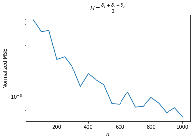
Example 1. Firstly we check the effectiveness of the deconvolution algorithm (Algorithm 4.1). For H=(δ1+δ4+δ9)/3,σ2=1H=(\delta_{1}+\delta_{4}+\delta_{9})/3,\sigma^{2}=1 and 20 equally spaced values of nn (starting from n=50n=50 and ending with n=1000n=1000) we solve the optimization problem described in Algorithm 4.1. We start from 10 randomly initialized points and keep the stationary point of the objective that leads to the smallest value. We plot in Figure 1, as a function of n,n, the resulting normalized mean squared error, which we define as

1n​∑i=1n(ti∗−λi)2Var⁡[H].\frac{\frac{1}{n}\sum_{i=1}^{n}(t_{i}^{*}-\lambda_{i})^{2}}{\operatorname{Var}\left[H\right]}.

We also present the recovered eigenvalues ti∗t_{i}^{*} versus i=1,⋯,ni=1,\cdots,n for the values n=250,500,750,1000.n=250,500,750,1000.

Refer to caption
(a) Algorithm 4.1 Objective
Refer to caption
(b) Recovered Eigenvalues
Figure 1. Algorithm 4.1 Experiment for H=(δ1+δ4+δ9)/3H=(\delta_{1}+\delta_{4}+\delta_{9})/3

Example 2. For a more complicated choice of spectral distribution HH we design the following experiment. We consider 200 randomly sampled points from circles centered at 0 with radii 0.5 and 1 respectively (presented with red and blue dots in the plot below). We add Gaussian noise with standard deviation 0.05 to the data. After generating those points, labeled as x1,⋯,x200∈ℝ2,x_{1},\cdots,x_{200}\in\mathbb{R}^{2}, we build the connectivity matrix A∈ℝ200×200A\in\mathbb{R}^{200\times 200} using the Gaussian kernel:

Ai​j=exp⁡(−‖xi−xj‖22​h2).A_{ij}=\exp{\left(-\frac{\left\lVert x_{i}-x_{j}\right\rVert^{2}}{2h^{2}}\right)}.

Here we choose h=0.1.h=0.1. We assume that we have access only to a matrix

A^=A+2200​Z,\hat{A}=A+\sqrt{\frac{2}{200}}Z,

where ZZ is a standard Gaussian Wigner matrix. This corresponds to the choice σ2=2.\sigma^{2}=2. We use Algorithm 4.1 to estimate the eigenvalues of A.A. Below we plot the sample eigevalues (that is the eigenvalues of A^\hat{A}), the true eigenvalues of AA and, finally, the estimated eigenvalues from the deconvolution algorithm. We see in Figure 2 that the reconstruction is very close.

Refer to caption
(a) n=200n=200 Generated Data Points
Refer to caption
(b) Eigenvalues
Figure 2. Algorithm 4.1 Experiment for the Connectivity Matrix created using a Gaussian Kernel with h=0.1.h=0.1.

Example 3. Finally, we consider an example with unknown noise level σ2.\sigma^{2}. In particular, we consider H=(δ5+δ10)/2,σ2=1,n=200.H=(\delta_{5}+\delta_{10})/2,\sigma^{2}=1,n=200. We take ZZ to have entries drawn from a Laplace distribution. This time σ2\sigma^{2} is unknown, so we have to use several choices σ^\hat{\sigma} in the optimization problem and choose the largest σ^\hat{\sigma} for which the objective is close to 0. Figure 3 indicates using σ^2\hat{\sigma}^{2} from 0.951 to 1.029. Refining the grid can give us an even closer estimate. We solve the optimization problem for σ^2=0.99,\hat{\sigma}^{2}=0.99, which is the midpoint between the two values of σ2\sigma^{2} from above.

Refer to caption
(a) Algorithm 4.1 Objective versus σ^2\hat{\sigma}^{2}
Refer to caption
(b) Eigenvalues for the estimated σ^2=0.99\hat{\sigma}^{2}=0.99
Figure 3. Algorithm 4.1 Experiment for H=(δ1+δ10)/2,σ=1.H=(\delta_{1}+\delta_{10})/2,\sigma=1. Here σ\sigma is unknown and is estimated from A^.\hat{A}.

6.2. Noisy Linear Systems of Equations.

The first application we consider is the following. We want to solve a linear system of equations of the form A​x=b,Ax=b, whose solution we denote x∗=A−1​b.x^{*}=A^{-1}b. The matrix AA is unknown. Instead we have access to a noisy estimate A^=A+σn−1/2Z,\hat{A}=A+\sigma n^{-1/2}Z, where A,ZA,Z satisfy the assumptions from Section 1. Solving A^​x=b\hat{A}x=b gives x=A^−1​b.x=\hat{A}^{-1}b. The problem is that A^−1\hat{A}^{-1} might be a very bad estimate of A−1A^{-1} and ill-conditioned. For this reason we suggest using x(f)=f⁡(A^)​b,x^{(f)}=f(\hat{A})b, where ff is a bounded continuous function on [h1,h2].[h_{1},h_{2}]. Our goal is to choose ff to minimize

limn→∞‖x(f)−x∗‖2n.\lim_{n\rightarrow\infty}\frac{\left\lVert x^{(f)}-x^{*}\right\rVert^{2}}{n}.

We study two different distributional assumptions on b.b.

  1. (1)

    b∼𝒩⁡(0,In)b\sim\mathcal{N}(0,I_{n}). In that case using Lemma 7.2 we see that:

    limn→∞‖x(f)−x∗‖2n=limn→∞‖(f⁡(A^)−A−1)​b‖2n=limn→∞‖f⁡(A^)−A−1‖F2n,\begin{split}\lim_{n\rightarrow\infty}\frac{\left\lVert x^{(f)}-x^{*}\right\rVert^{2}}{n}=\lim_{n\rightarrow\infty}\frac{\left\lVert(f(\hat{A})-A^{-1})b\right\rVert^{2}}{n}=\lim_{n\rightarrow\infty}\frac{\left\lVert f(\hat{A})-A^{-1}\right\rVert_{F}^{2}}{n},\end{split} (8)

    which is minimized for f⁡(x)=f1/t∗​(x).f(x)=f^{*}_{1/t}(x).

  2. (2)

    b=A​x∗,x∗∼𝒩⁡(0,In)b=Ax^{*},x^{*}\sim\mathcal{N}(0,I_{n}). Similarly using Lemma 7.2 we see that:

    limn→∞‖x(f)−x∗‖2n=limn→∞‖(f⁡(A^)​A−In)​x∗‖2n=limn→∞‖f⁡(A^)​A−In‖F2n.\begin{split}\lim_{n\rightarrow\infty}\frac{\left\lVert x^{(f)}-x^{*}\right\rVert^{2}}{n}=\lim_{n\rightarrow\infty}\frac{\left\lVert(f(\hat{A})A-I_{n})x^{*}\right\rVert^{2}}{n}=\lim_{n\rightarrow\infty}\frac{\left\lVert f(\hat{A})A-I_{n}\right\rVert_{F}^{2}}{n}.\end{split} (9)

    Using exactly the same argument as in Proposition 3.1 we see that the limit is almost surely

    1−2​∫f⁡(x)​vt​(x)π​𝑑x+∫f2​(x)​vt2​(x)π​𝑑x,1-2\int f(x)\frac{v_{t}(x)}{\pi}dx+\int f^{2}(x)\frac{v_{t^{2}}(x)}{\pi}dx,

    which is minimized for f⁡(x)=ft∗​(x)/ft2∗​(x).f(x)=f_{t}^{*}(x)/f_{t^{2}}^{*}(x).

For H=(δ1+δ10)/2,n=500H=(\delta_{1}+\delta_{10})/2,n=500 we plot in Figure 4 the normalized mean-squared-error (which we define as ‖x(f)−x∗‖2/‖x∗‖2\left\lVert x^{(f)}-x^{*}\right\rVert^{2}/\left\lVert x^{*}\right\rVert^{2}) for several values of σ2.\sigma^{2}.

Refer to caption
(a) b∼𝒩⁡(0,In)b\sim\mathcal{N}(0,I_{n})
Refer to caption
(b) x∗∼𝒩⁡(0,In)x^{*}\sim\mathcal{N}(0,I_{n})
Figure 4. ‖x(f)−x∗‖2/‖x∗‖2\left\lVert x^{(f)}-x^{*}\right\rVert^{2}/\left\lVert x^{*}\right\rVert^{2} for different choices of ff and H=(δ1+δ10)/2.H=(\delta_{1}+\delta_{10})/2.

We repeat the experiment for H=(δ1+δ4+δ9)/3,n=200.H=(\delta_{1}+\delta_{4}+\delta_{9})/3,n=200. The results can be seen in Figure 5.

Refer to caption
(a) b∼𝒩⁡(0,In)b\sim\mathcal{N}(0,I_{n})
Refer to caption
(b) x∗∼𝒩⁡(0,In)x^{*}\sim\mathcal{N}(0,I_{n})
Figure 5. ‖x(f)−x∗‖2/‖x∗‖2\left\lVert x^{(f)}-x^{*}\right\rVert^{2}/\left\lVert x^{*}\right\rVert^{2} for different choices of ff and H=(δ1+δ4+δ9)/3.H=(\delta_{1}+\delta_{4}+\delta_{9})/3.

In both cases we see that A^\hat{A} becomes eventually ill-conditioned, if σ2\sigma^{2} increases. As expected, if b∼𝒩⁡(0,In)b\sim\mathcal{N}(0,I_{n}) the first shrinkage outperforms the second at all noise levels, while for x∗∼𝒩⁡(0,In)x^{*}\sim\mathcal{N}(0,I_{n}) the opposite is true.

6.3. Experiments for Algorithm 3.1

We consider the problem of estimating A,A−1A,A^{-1} and A\sqrt{A} in Frobenius norm, when we only have access to A^.\hat{A}. For n=500n=500 and several values of σ\sigma we generate A^=A+σn−1/2Z,\hat{A}=A+\sigma n^{-1/2}Z, where ZZ is a standard Gaussian Wigner matrix. Here AA is chosen as a diagonal matrix with diagonal entries chosen uniformly at random from {1,4,9}.\{1,4,9\}. We plot for h⁡(t)=t,h⁡(t)=1/t,h⁡(t)=th(t)=t,h(t)=1/t,h(t)=\sqrt{t} the oracle error and the error that can be achieved by using Algorithm 4.1 to recover the eigenvalues of AA and Algorithm 3.1 with K=1K=1 to perform nonlinear shrinkage. We see that in all cases the error achieved by our algorithm is very close to the oracle. For σ2\sigma^{2} large, notice that the problem of eigenvalue recovery for AA becomes increasingly harder, hence the error in estimation of λ1,⋯,λn\lambda_{1},\cdots,\lambda_{n} increases. This can lead to problems for the function h⁡(t)=1/th(t)=1/t which is unbounded near 0, hence we clip all the recovered eigenvalues that we get from Algorithm 4.1 to be at least 0.3. Notice that for h⁡(t)=1/t,h⁡(t)=th(t)=1/t,h(t)=\sqrt{t} we do not plot the no shrinkage

Refer to caption
(a) Algorithm 3.1 for h⁡(t)=t.h(t)=t.
Refer to caption
(b) Algorithm 3.1 for h⁡(t)=1/t.h(t)=1/t.
Refer to caption
(c) Algorithm 3.1 for h⁡(t)=t.h(t)=\sqrt{t}.
Figure 6. Algorithm 3.1 Experiment for H=(δ1+δ4+δ9)/3.H=(\delta_{1}+\delta_{4}+\delta_{9})/3. We plot the oracle and shrinkage errors versus σ\sigma for h⁡(t)=t,1/t,t.h(t)=t,1/t,\sqrt{t}.

7. Proofs

7.1. Proofs for Section 2

We start by presenting a well-known lemma for the tails of a standard Gaussian random variable.

Lemma 7.1.

For any M>0M>0 and Z∼𝒩⁡(0,1)Z\sim\mathcal{N}(0,1) we have

ℙ(|Z|>M)≤2M−1exp(−x2/2).\mathbb{P}(\left\lvert Z\right\rvert>M)\leq 2M^{-1}\exp{(-x^{2}/2)}.
Proof.

We have

ℙ(|Z|>M)=2ℙ(Z>M)=2∫M∞exp(−x2/2)dx≤2∫M∞xMexp(−x2/2)dx=2M−1exp(−x2/2).\begin{split}\mathbb{P}(\left\lvert Z\right\rvert>M)=2\mathbb{P}(Z>M)=2\int_{M}^{\infty}\exp{(-x^{2}/2)}dx\\ \leq 2\int_{M}^{\infty}\frac{x}{M}\exp{(-x^{2}/2)}dx=2M^{-1}\exp{(-x^{2}/2)}.\end{split} (10)

∎

We will need the following lemma which is adapted from Lemma 7.8, Lemma 7.9 and Lemma 7.10 from Erdős and Yau 2017.

Lemma 7.2.

Let q≥2q\geq 2 and X1,⋯,XN,Y1,⋯,YNX_{1},\cdots,X_{N},Y_{1},\cdots,Y_{N} be independent random variables with mean 0, variance 1 and 2​q2q-th moment bounded by c0c_{0}. Then, for any deterministic (bi)1≤i≤N,(ai​j)1≤i,j≤N(b_{i})_{1\leq i\leq N},(a_{ij})_{1\leq i,j\leq N} we have for some positive constant Cq=Cq​(c0)C_{q}=C_{q}(c_{0}):

‖∑ibi​(Xi2−1)‖q≤Cq​(∑i|bi|2)12\left\lVert\sum_{i}b_{i}(X_{i}^{2}-1)\right\rVert_{q}\leq C_{q}(\sum_{i}\left\lvert b_{i}\right\rvert^{2})^{\frac{1}{2}} (11)
‖∑i,jai​j​Xi​Yj‖q≤Cq​(∑i,jai​j2)12\left\lVert\sum_{i,j}a_{ij}X_{i}Y_{j}\right\rVert_{q}\leq C_{q}(\sum_{i,j}a_{ij}^{2})^{\frac{1}{2}} (12)
‖∑i≠jai​j​Xi​Xj‖q≤Cq​(∑i≠jai​j2)12\left\lVert\sum_{i\neq j}a_{ij}X_{i}X_{j}\right\rVert_{q}\leq C_{q}(\sum_{i\neq j}a_{ij}^{2})^{\frac{1}{2}} (13)
Proof of Theorem 2.2.

The proof involves two main steps.

  1. (1)

    Step 1: Show that the theorem holds for if Z∼G​O​E​(n).Z\sim GOE(n).

  2. (2)

    Step 2: Reduce the problem to the case of bounded random variables as entries of Z.Z.

  3. (3)

    Step 3: Show that the results are universally true and independent of the distribution of ZZ as long as Z,AZ,A are asymptotically free.

Step 1: For Z∼G​O​E​(n)Z\sim GOE(n) (which is invariant under conjugation by an orthogonal matrix) it is enough to consider the case of diagonal matrix A.A. If A=diag⁡(A1,⋯,An),A=\operatorname{diag}(A_{1},\cdots,A_{n}), then using the Schur complement formula we have that the ii-th diagonal entry of h⁡(A)​(A^−z)−1h(A)\left(\hat{A}-z\right)^{-1} is given by

h(Ai)/(Ai−z−σn−1/2Zi​i−σ2n−1ai⊺(A−i+n−1/2Z−i−z)−1ai).h(A_{i})/\left(A_{i}-z-\sigma n^{-1/2}Z_{ii}-\sigma^{2}n^{-1}a_{i}^{\intercal}\left(A_{-i}+n^{-1/2}Z_{-i}-z\right)^{-1}a_{i}\right).

Here A−iA_{-i} is the (n−1)×(n−1)(n-1)\times(n-1) matrix that we get if we omit the ii-th element AiA_{i} of A,A, ai∈ℝ(n−1)a_{i}\in\mathbb{R}^{(n-1)} the ii-th row of ZZ if we omit the diagonal element.

We have from Lemma 7.1 for any fixed ϵ>0\epsilon>0 and n≥ϵ−2:n\geq\epsilon^{-2}:

ℙ(max1≤i≤n|Zi​i|>ϵn)≤nℙ(|Zi​i|>ϵn)=𝒪(nexp(−nϵ2/2)).\mathbb{P}\left(\max_{1\leq i\leq n}\left\lvert Z_{ii}\right\rvert>\epsilon\sqrt{n}\right)\leq n\mathbb{P}\left(\left\lvert Z_{ii}\right\rvert>\epsilon\sqrt{n}\right)=\mathcal{O}\left(n\exp{(-n\epsilon^{2}/2)}\right).

Since ϵ\epsilon was arbitrary, we conclude by the Borel-Cantelli lemma that

max1≤i≤n⁡|Zi​i|/n→a.s.0.\max_{1\leq i\leq n}\left\lvert Z_{ii}\right\rvert/\sqrt{n}\xrightarrow{a.s.}0.

Similarly, by Lemma 7.2 for q=3q=3,

max1≤i≤nn−1|ai⊺(A−i+σn−1/2Z−i−z)−1ai−tr((A−i+σn−1/2Z−i−z)−1)|.\max_{1\leq i\leq n}n^{-1}\left\lvert a_{i}^{\intercal}\left(A_{-i}+\sigma n^{-1/2}Z_{-i}-z\right)^{-1}a_{i}-tr\left(\left(A_{-i}+\sigma n^{-1/2}Z_{-i}-z\right)^{-1}\right)\right\rvert.

Using the Cauchy interlacing formula (Tao 2012), we see that it must also be true that

max1≤i≤n|n−1tr((A−i+σn−1/2Z−i−z)−1)−mμ^(z)|→a.s.0,\begin{split}\max_{1\leq i\leq n}\left\lvert n^{-1}tr\left(\left(A_{-i}+\sigma n^{-1/2}Z_{-i}-z\right)^{-1}\right)-m_{\hat{\mu}}(z)\right\rvert\xrightarrow{a.s.}0,\end{split} (14)

as for fixed z∈ℂ+z\in\mathbb{C}^{+} the differences

|tr((A−i+σn−1/2Z−i−z)−1)−tr((A+σn−1/2Z−z)−1)(z)|\left\lvert tr\left(\left(A_{-i}+\sigma n^{-1/2}Z_{-i}-z\right)^{-1}\right)-tr\left(\left(A+\sigma n^{-1/2}Z-z\right)^{-1}\right)(z)\right\rvert

are going to be uniformly bounded (due to the interlacing phenomenon).

As a consequence, we see that

n−1​t​r​(h⁡(A)​(A^−z)−1)=o⁡(1)+∑i=1nh⁡(Ai)ti−z−σ2​mμ^​(z),n^{-1}tr\left(h(A)\left(\hat{A}-z\right)^{-1}\right)=o{(1)}+\sum_{i=1}^{n}\frac{h(A_{i})}{t_{i}-z-\sigma^{2}m_{\hat{\mu}}(z)},

which proves the result for z∈ℂ+z\in\mathbb{C}^{+} and Z∼G​O​E​(n).Z\sim GOE(n).

Step 2: Fix M>0.M>0. For this step we assume, in order to slightly simplify the formulas, that without loss of generality that σ=1.\sigma=1. Define Zi,j(M)=Zi​j​𝕀|Zi​j|<M.Z_{i,j}^{(M)}=Z_{ij}\mathbb{I}_{\left\lvert Z_{ij}\right\rvert<M}. We also define A^(M)=A+n−1/2Z(M).\hat{A}^{(M)}=A+n^{-1/2}Z^{(M)}. We have

|n−1​t​r​(h⁡(A)​(A^(M)−z)−1)−n−1​t​r​(h⁡(A)​(A^−z)−1)|=|t​r​(h⁡(A)​(A^−z)−1​(Z−Z(M))​(A^(M)−z)−1)|n​n=|t​r​((A^(M)−z)−1​h​(A)​(A^−z)−1​(Z−Z(M)))|n​n≤‖(A^(M)−z)−1​h​(A)​(A^−z)−1‖o​p​‖(Z−Z(M))‖Fn.\begin{split}\left\lvert n^{-1}tr\left(h(A)(\hat{A}^{(M)}-z)^{-1}\right)-n^{-1}tr\left(h(A)(\hat{A}-z)^{-1}\right)\right\rvert\\ =\frac{\left\lvert tr\left(h(A)(\hat{A}-z)^{-1}(Z-Z^{(M)})(\hat{A}^{(M)}-z)^{-1}\right)\right\rvert}{n\sqrt{n}}\\ =\frac{\left\lvert tr\left((\hat{A}^{(M)}-z)^{-1}h(A)(\hat{A}-z)^{-1}(Z-Z^{(M)})\right)\right\rvert}{n\sqrt{n}}\\ \leq\frac{\left\lVert(\hat{A}^{(M)}-z)^{-1}h(A)(\hat{A}-z)^{-1}\right\rVert_{op}\left\lVert(Z-Z^{(M)})\right\rVert_{F}}{n}.\end{split} (15)

Notice that here we have used the fact that for two n×nn\times n matrices M1,M2M_{1},M_{2} we have

|t​r​(M1​M2)|≤‖M1‖F​‖M2‖F≤n​‖M1‖o​p​‖M2‖F,\left\lvert tr\left(M_{1}M_{2}\right)\right\rvert\leq\left\lVert M_{1}\right\rVert_{F}\left\lVert M_{2}\right\rVert_{F}\leq\sqrt{n}\left\lVert M_{1}\right\rVert_{op}\left\lVert M_{2}\right\rVert_{F},

where the first inequality follows from Cauchy-Schwartz in ℝn×n\mathbb{R}^{n\times n} and the second one from the fact that the Frobenius norm of a real matrix is the l2−l_{2}-norm of its singular values.

We conclude from (15) that for a fixed bounded continuous function and a fixed complex number zz in the upper half-plane we have

|n−1​t​r​(h⁡(A)​(A^(M)−z)−1)−n−1​t​r​(h⁡(A)​(A^−z)−1)|=𝒪⁡(n−1​‖Z−Z(M)‖F).\begin{split}\left\lvert n^{-1}tr\left(h(A)(\hat{A}^{(M)}-z)^{-1}\right)-n^{-1}tr\left(h(A)(\hat{A}-z)^{-1}\right)\right\rvert=\mathcal{O}\left(n^{-1}\left\lVert Z-Z^{(M)}\right\rVert_{F}\right).\end{split} (16)

We now observe that

𝔼⁡[‖(Z−Z(M))‖F2]=n2​𝔼​[Z112;|Z11|≥M]\mathbb{E}\left[\left\lVert\left(Z-Z^{(M)}\right)\right\rVert_{F}^{2}\right]=n^{2}\mathbb{E}\left[Z_{11}^{2};\left\lvert Z_{11}\right\rvert\geq M\right]

and

Var⁡[‖Z−Z(M)‖F2]=𝒪⁡(n2​𝔼​[Z114;|Z11|>M]).\operatorname{Var}\left[\left\lVert Z-Z^{(M)}\right\rVert_{F}^{2}\right]=\mathcal{O}\left(n^{2}\mathbb{E}\left[Z_{11}^{4};\left\lvert Z_{11}\right\rvert>M\right]\right).

Fix any ϵ>0\epsilon>0 and take MM large enough such that 𝔼⁡[Z112;|Z11|>M]≤ϵ2/2\mathbb{E}[Z_{11}^{2};\left\lvert Z_{11}\right\rvert>M]\leq\epsilon^{2}/2 and 𝔼⁡[Z114;|Z11|>M]≤1.\mathbb{E}\left[Z_{11}^{4};\left\lvert Z_{11}\right\rvert>M\right]\leq 1. Then we have

ℙ⁡(n−1​‖Z−Z(M)‖F>ϵ)=ℙ⁡(n−2​‖Z−Z(M)‖F2>ϵ2)≤ℙ⁡(n−2​‖Z−Z(M)‖F2−𝔼⁡[n−2​‖Z−Z(M)‖F2]>ϵ2/2)=𝒪⁡(n−2​ϵ−4).\begin{split}&\mathbb{P}\left(n^{-1}\left\lVert Z-Z^{(M)}\right\rVert_{F}>\epsilon\right)=\mathbb{P}\left(n^{-2}\left\lVert Z-Z^{(M)}\right\rVert_{F}^{2}>\epsilon^{2}\right)\\ &\leq\mathbb{P}\left(n^{-2}\left\lVert Z-Z^{(M)}\right\rVert_{F}^{2}-\mathbb{E}\left[n^{-2}\left\lVert Z-Z^{(M)}\right\rVert_{F}^{2}\right]>\epsilon^{2}/2\right)=\mathcal{O}\left(n^{-2}\epsilon^{-4}\right).\end{split} (17)

Using the Borel-Cantelli lemma we conclude that. almost surely, n−1​‖Z−Z(M)‖F≤ϵn^{-1}\left\lVert Z-Z^{(M)}\right\rVert_{F}\leq\epsilon eventually. Using (15) we see that for MM large enough we have eventually almost surely

|n−1​t​r​(h⁡(A)​(A^(M)−z)−1)−n−1​t​r​(h⁡(A)​(A^−z)−1)|≤ϵ​‖(A^(M)−z)−1​h​(A)​(A^−z)−1‖o​p≤ϵ​I​m​(z)−2​‖h‖∞.\begin{split}\left\lvert n^{-1}tr\left(h(A)(\hat{A}^{(M)}-z)^{-1}\right)-n^{-1}tr\left(h(A)(\hat{A}-z)^{-1}\right)\right\rvert\\ \leq\epsilon\left\lVert(\hat{A}^{(M)}-z)^{-1}h(A)(\hat{A}-z)^{-1}\right\rVert_{op}\leq\epsilon Im(z)^{-2}\left\lVert h\right\rVert_{\infty}.\end{split} (18)

To finish this step, we define μM=𝔼⁡[Zi​j(M)],σM=Var⁡[Zi​j(M)]\mu_{M}=\mathbb{E}\left[Z_{ij}^{(M)}\right],\sigma_{M}=\sqrt{\operatorname{Var}\left[Z_{ij}^{(M)}\right]} and Z~i​j=(Zi​j(M)−μM)/σM,\tilde{Z}_{ij}=\left(Z_{ij}^{(M)}-\mu_{M}\right)/\sigma_{M}, which are random variables with mean 0 and variance 1. A similar argument shows that, if A~=A+n−1/2Z~\tilde{A}=A+n^{-1/2}\tilde{Z} and MM is large enough, then eventually almost surely we have

|n−1​t​r​(h⁡(A)​(A^(M)−z)−1)−n−1​t​r​(h⁡(A)​(A~−z)−1)|≤ϵ.\left\lvert n^{-1}tr\left(h(A)\left(\hat{A}^{(M)}-z\right)^{-1}\right)-n^{-1}tr\left(h(A)\left(\tilde{A}-z\right)^{-1}\right)\right\rvert\leq\epsilon. (19)

To see why, using the same bound as in (15), we see that

|n−1​t​r​(h⁡(A)​(A^(M)−z)−1)−n−1​t​r​(h⁡(A)​(A~−z)−1)|≤‖(A^(M)−z)−1​h​(A)​(A~−z)−1‖o​p​‖Z~−Z(M)‖Fn≤n−1​‖h‖∞​I​m​(z)−2​‖Z~−Z(M)‖F.\begin{split}&\left\lvert n^{-1}tr\left(h(A)\left(\hat{A}^{(M)}-z\right)^{-1}\right)-n^{-1}tr\left(h(A)\left(\tilde{A}-z\right)^{-1}\right)\right\rvert\leq\\ &\frac{\left\lVert\left(\hat{A}^{(M)}-z\right)^{-1}h(A)\left(\tilde{A}-z\right)^{-1}\right\rVert_{op}\left\lVert\tilde{Z}-Z^{(M)}\right\rVert_{F}}{n}\leq n^{-1}\left\lVert h\right\rVert_{\infty}Im(z)^{-2}\left\lVert\tilde{Z}-Z^{(M)}\right\rVert_{F}.\end{split} (20)

It remains to bound Z~−Z(M)\tilde{Z}-Z^{(M)} in Frobenius norm. Let e=(1,⋯,1)⊺∈ℝn.e=(1,\cdots,1)^{\intercal}\in\mathbb{R}^{n}. Then,

Z~−Z(M)=Z~(M)​(1−σM−1)−μMσM​e​e⊺.\tilde{Z}-Z^{(M)}=\tilde{Z}^{(M)}(1-\sigma_{M}^{-1})-\frac{\mu_{M}}{\sigma_{M}}ee^{\intercal}.

Using this we get

‖Z~−Z(M)‖F2=(1−σM−1)2​‖Z(M)‖F2−2​μMσM​(1−σM−1)​e⊺​Z(M)​e+n2​μM2σM2≤n2​μM2σM2−2​μMσM​(1−σM−1)​e⊺​Z(M)​e+(1−σM−1)​(‖Z‖F+‖Z−Z(M)‖F)2\begin{split}\left\lVert\tilde{Z}-Z^{(M)}\right\rVert_{F}^{2}=(1-\sigma_{M}^{-1})^{2}\left\lVert Z^{(M)}\right\rVert_{F}^{2}-2\frac{\mu_{M}}{\sigma_{M}}(1-\sigma_{M}^{-1})e^{\intercal}Z^{(M)}e+n^{2}\frac{\mu_{M}^{2}}{\sigma_{M}^{2}}\\ \leq n^{2}\frac{\mu_{M}^{2}}{\sigma_{M}^{2}}-2\frac{\mu_{M}}{\sigma_{M}}(1-\sigma_{M}^{-1})e^{\intercal}Z^{(M)}e+(1-\sigma_{M}^{-1})\left(\left\lVert Z\right\rVert_{F}+\left\lVert Z-Z^{(M)}\right\rVert_{F}\right)^{2}\end{split} (21)

Now we know that:

  1. (1)

    limM→∞μM=0\lim_{M\rightarrow\infty}\mu_{M}=0 and limM→∞σM=1\lim_{M\rightarrow\infty}\sigma_{M}=1 from the dominated convergence theorem.

  2. (2)

    n−1​‖Z−Z(M)‖n^{-1}\left\lVert Z-Z^{(M)}\right\rVert can be made arbitrarily small eventually (by choosing MM large enough), using (17) and the Borel-Cantelli lemma.

  3. (3)

    n−1​‖Z‖F≤n−1​‖Z‖o​p,n^{-1}\left\lVert Z\right\rVert_{F}\leq\sqrt{n^{-1}\left\lVert Z\right\rVert_{op}}, which converges to 22 almost surely (Tao 2012).

  4. (4)

    Finally,

    n−2​e⊺​Z(M)​e=∑1≤i,j≤nZi​j​𝕀|Zi​j|<Mn2→a.s.𝔼⁡[Z11;|Z11|<M]n^{-2}e^{\intercal}Z^{(M)}e=\frac{\sum_{1\leq i,j\leq n}Z_{ij}\mathbb{I}_{\left\lvert Z_{ij}\right\rvert<M}}{n^{2}}\xrightarrow{a.s.}\mathbb{E}\left[Z_{11};\left\lvert Z_{11}\right\rvert<M\right]

    by the strong law of large numbers.

Taking all of the above into consideration, we see that for MM large enough we see that for MM large enough we have eventually almost surely that the bound from (19) is true. Since Z~\tilde{Z} is a Wigner ensemble with bounded entries, we have reduced the problem to the case of bounded random variables.

Step 3: We now show that under the assumptions in Subsection 1.1 the theorem is also true. The idea is to show, using free-probabilistic tools, that if Z~\tilde{Z} is a Wigner ensemble with all moments finite, the the limit of the trace functionals of interest depends on the noise distribution via only its first two moments. First of all, notice that it is enough to prove the result for a polynomial hh and the extend to a general continuous function by a simple density argument. As a result, it is enough to consider h⁡(t)=tk,k∈ℕh(t)=t^{k},k\in\mathbb{N} and show that n−1​t​r​(Ak​(A^−z)−1)n^{-1}tr\left(A^{k}\left(\hat{A}-z\right)^{-1}\right) has a limit almost surely and the limit does not depend on the distribution of Z.Z. Similarly, it is enough to show that for any m∈ℕm\in\mathbb{N} the trace functional n−1​t​r​(Ak​A^m)n^{-1}tr\left(A^{k}\hat{A}^{m}\right) has a limit almost surely and the limit does not depend on the distribution of Z.Z. Writing A^m=(A+σn−1/2Z)m\hat{A}^{m}=\left(A+\sigma n^{-1/2}Z\right)^{m} and expanding in monomial terms we see that n−1​t​r​(Ak​A^m)n^{-1}tr\left(A^{k}\hat{A}^{m}\right) is the sum of a finite number of terms all of which have the form n−1tr(An1(σn−1/2Z)m1⋯Ans(n−1/2Z)ms)n^{-1}tr\left(A^{n_{1}}(\sigma n^{-1/2}Z)^{m_{1}}\cdots A^{n_{s}}\left(n^{-1/2}Z\right)^{m_{s}}\right) for some s≥1s\geq 1 and nonnegative integers n1,m1,⋯,ns,ms.n_{1},m_{1},\cdots,n_{s},m_{s}. Since ZZ is a Wigner ensemble and AA is independent of Z,Z, we conclude that A,n−1/2ZA,n^{-1/2}Z are almost surely asymptotically free (Theorem 20 in Mingo and Speicher 2017). As a consequence, we have that all terms of the form n−1tr(An1(σn−1/2Z)m1⋯Ans(n−1/2Z)ms)n^{-1}tr\left(A^{n_{1}}(\sigma n^{-1/2}Z)^{m_{1}}\cdots A^{n_{s}}\left(n^{-1/2}Z\right)^{m_{s}}\right) converge almost surely and the limit depends only on the limiting spectral distributions of A,n−1/2Z,A,n^{-1/2}Z, which are given by HH and a semicircular distribution respectively. In particular, the limit is independent of the distribution of Z.Z. We conclude that the limit is the same as with the Gaussian assumption on Z.Z. This completes the proof. ∎

7.2. Proofs for Section 3

Proof of Theorem 3.1.

First of all, let ff be an analytic function on the complex plane. Then, we have using Cauchy’s integral formula:

t​r​(f⁡(A^)​h​(A))n=−12​π​i∮|z|=Rt​r​(h⁡(A)​(A^−z)−1)nf(z)dz,\frac{tr\left(f(\hat{A})h(A)\right)}{n}=-\frac{1}{2\pi i}\oint_{\left\lvert z\right\rvert=R}\frac{tr\left(h(A)\left(\hat{A}-z\right)^{-1}\right)}{n}f(z)dz,

where the integral is considered on a fixed circle centered at 00 with radius RR such that eventually ‖A^‖o​p≤R/2.\left\lVert\hat{A}\right\rVert_{op}\leq R/2. Consider

Rn​(z)=t​r​(h⁡(A)​(A^−z)−1)nR_{n}(z)=\frac{tr\left(h(A)\left(\hat{A}-z\right)^{-1}\right)}{n}

and for a fixed zz let us denote by R∞​(z)R_{\infty}(z) the almost sure limit of Rn​(z)R_{n}(z) described in Theorem 2.2. Then, for nn large enough we have almost surely that:

|Rn​(z)|=|t​r​(h⁡(A)​(A^−z)−1)n|≤‖h⁡(A)‖o​p(R−R/2)=2​R−1​‖h⁡(A)‖o​p,\left\lvert R_{n}(z)\right\rvert=\left\lvert\frac{tr\left(h(A)\left(\hat{A}-z\right)^{-1}\right)}{n}\right\rvert\leq\frac{\left\lVert h(A)\right\rVert_{op}}{(R-R/2)}=2R^{-1}\left\lVert h(A)\right\rVert_{op},

and

|Rn′​(z)|=|t​r​(h⁡(A)​(A^−z)−2)n|≤‖h⁡(A)‖o​p(R−R/2)2=4​R−2​‖h⁡(A)‖o​p,\left\lvert R_{n}^{\prime}(z)\right\rvert=\left\lvert\frac{tr\left(h(A)\left(\hat{A}-z\right)^{-2}\right)}{n}\right\rvert\leq\frac{\left\lVert h(A)\right\rVert_{op}}{(R-R/2)^{2}}=4R^{-2}\left\lVert h(A)\right\rVert_{op},

so on the circle {z∈ℂ:|z|=R}\{z\in\mathbb{C}:\left\lvert z\right\rvert=R\} the sequence of functions {Rn​(z)}n≥1\{R_{n}(z)\}_{n\geq 1} almost surely consists of functions that are uniformly bounded and equicontinuous. Fix some ϵ>0\epsilon>0 and consider a finite subset C⊂{z∈ℂ:|z|=R}C\subset\{z\in\mathbb{C}:\left\lvert z\right\rvert=R\} such that for any z∈ℂz\in\mathbb{C} with |z|=R\left\lvert z\right\rvert=R there exists z~∈C\tilde{z}\in C such that |z−z~|<ϵ.\left\lvert z-\tilde{z}\right\rvert<\epsilon. Since for any such z,z~z,\tilde{z} we have

|Rn​(z)−R∞​(z)|≤|Rn​(z)−Rn​(z~)|+|Rn​(z~)−R∞​(z~)|+|R∞​(z~)−R∞​(z)|\left\lvert R_{n}(z)-R_{\infty}(z)\right\rvert\leq\left\lvert R_{n}(z)-R_{n}(\tilde{z})\right\rvert+\left\lvert R_{n}(\tilde{z})-R_{\infty}(\tilde{z})\right\rvert+\left\lvert R_{\infty}(\tilde{z})-R_{\infty}(z)\right\rvert
=𝒪⁡(ϵ+supz~∈C|Rn​(z~)−R∞​(z~)|),=\mathcal{O}\left(\epsilon+\sup_{\tilde{z}\in C}\left\lvert R_{n}(\tilde{z})-R_{\infty}(\tilde{z})\right\rvert\right),

we know that almost surely

lim supsup|z|=R|Rn​(z)−R∞​(z)|=𝒪⁡(ϵ).\limsup\sup_{\left\lvert z\right\rvert=R}\left\lvert R_{n}(z)-R_{\infty}(z)\right\rvert=\mathcal{O}(\epsilon).

Since ϵ\epsilon was arbitrary we conclude that Rn→a.s.R∞R_{n}\xrightarrow{a.s.}R_{\infty} uniformly on {z∈ℂ:|z|=R}.\{z\in\mathbb{C}:\left\lvert z\right\rvert=R\}. Using this result we see that

t​r​(h⁡(A)​f​(A^))n→a.s.−12​π​i∮|z|=RR∞(z)f(z)dz=−12​π​i∮ΓδR∞(z)f(z)dz,\frac{tr\left(h(A)f\left(\hat{A}\right)\right)}{n}\xrightarrow{a.s.}{-\frac{1}{2\pi i}}\oint_{\left\lvert z\right\rvert=R}R_{\infty}(z)f(z)dz=-\frac{1}{2\pi i}\oint_{\Gamma_{\delta}}R_{\infty}(z)f(z)dz,

where we have changed the integral to be on a counterclockwise curve Γδ\Gamma_{\delta} which we take to be a rectangle with vertices ±R±i​δ.\pm R\pm i\delta. Taking δ↓0\delta\downarrow 0 we get

−12​π​i∮R∞(z)f(z)dz=−12​π​ilimδ↓0[∫−RRR∞(x−iδ)f(x−iδ)dx−∫−RRR∞(x+iδ)f(x+iδ)]=∫vh​(x)π​f​(x)​dx.\begin{split}&-\frac{1}{2\pi i}\oint R_{\infty}(z)f(z)dz\\ &=-\frac{1}{2\pi i}\lim_{\delta\downarrow 0}\left[\int_{-R}^{R}R_{\infty}(x-i\delta)f(x-i\delta)dx-\int_{-R}^{R}R_{\infty}(x+i\delta)f(x+i\delta)\right]\\ &=\int\frac{v_{h}(x)}{\pi}f(x)dx.\end{split} (22)

In other words, we have shown that

t​r​(f⁡(A^)​h​(A))n→a.s.∫vh​(x)π​f​(x)​𝑑x\frac{tr\left(f(\hat{A})h(A)\right)}{n}\xrightarrow{a.s.}\int\frac{v_{h}(x)}{\pi}f(x)dx

for ff analytic. Using a simple density argument we see that this result is actually true for any function ff that is continuous and bounded in an open set that contains the support of μH,σ2\mu_{H,\sigma^{2}} and eventually all the eigenvalues of A^.\hat{A}.

We now see that

‖f⁡(A^)−h⁡(A)‖F2n=‖f⁡(A^)‖F2−2​t​r​(f⁡(A^​h​(A))+‖h⁡(A)‖F2)n→a.s.∫f2​(x)​v⁡(x)π​dx−2​∫vh​(x)π​f​(x)​dx+∫h2​(x)​dH​(x).\begin{split}\frac{\left\lVert f(\hat{A})-h(A)\right\rVert_{F}^{2}}{n}=\frac{\left\lVert f(\hat{A})\right\rVert_{F}^{2}-2tr\left(f(\hat{A}h(A))+\left\lVert h(A)\right\rVert_{F}^{2}\right)}{n}\\ \xrightarrow{a.s.}\int f^{2}(x)\frac{v(x)}{\pi}dx-2\int\frac{v_{h}(x)}{\pi}f(x)dx+\int h^{2}(x)dH(x).\end{split} (23)

Minimizing over ff we see that for xx in the support of μH,σ2\mu_{H,\sigma^{2}} the minimizer satisfies f∗​(x)=vh​(x)/v⁡(x).f^{*}(x)=v_{h}(x)/v(x). This completes the proof. ∎

Proof of Corollary 3.1.
  1. (1)

    We have

    ∫t​d​H​(t)t−z−σ2​mμ^​(z)=1+∫z+σ2​mμ^​(z)t−z−σ2​mμ^​(z)=1+(z+σ2​mμ^​(z))​mμ^​(z),\int\frac{tdH(t)}{t-z-\sigma^{2}m_{\hat{\mu}}(z)}=1+\int\frac{z+\sigma^{2}m_{\hat{\mu}}(z)}{t-z-\sigma^{2}m_{\hat{\mu}}(z)}=1+(z+\sigma^{2}m_{\hat{\mu}}(z))m_{\hat{\mu}}(z),

    where the last equality follows from Proposition 2.1.

  2. (2)

    Using

    1t⁡(t−z−σ2​mμ^​(z))=1z+σ2​mμ^​(z)​[1t−z​σ2​mμ^​(z)−1t],\frac{1}{t(t-z-\sigma^{2}m_{\hat{\mu}}(z))}=\frac{1}{z+\sigma^{2}m_{\hat{\mu}}(z)}\left[\frac{1}{t-z\sigma^{2}m_{\hat{\mu}}(z)}-\frac{1}{t}\right],

    we have

    ∫d​H​(t)t⁡(t−z−σ2​mμ^​(z))=mμ^​(z)−mH​(0)z+σ2​mμ^​(z),\int\frac{dH(t)}{t(t-z-\sigma^{2}m_{\hat{\mu}}(z))}=\frac{m_{\hat{\mu}}(z)-m_{H}(0)}{z+\sigma^{2}m_{\hat{\mu}}(z)},

    so the formula for the asymptotically optimal shrinkage for A−1A^{-1} follows.

  3. (3)

    We have

    ∫t2​d​H​(t)t−z−σ2​mμ^​(z)=∫t2−(z+σ2​mμ^​(z))2t−z−σ2​mμ^​(z)​𝑑H​(t)+(z+σ2​mμ^​(z))2​∫d​H​(t)t−z−σ2​mμ^​(z)=∫(t+z+σ2​mμ^​(z))​dH​(t)+(z+σ2​mμ^​(z))2​mμ^​(z)=∫t​dH​(t)+z+σ2​mμ^​(z)+(z+σ2​mμ^​(z))2​mμ^​(z).\begin{split}&\int\frac{t^{2}dH(t)}{t-z-\sigma^{2}m_{\hat{\mu}}(z)}\\ &=\int\frac{t^{2}-(z+\sigma^{2}m_{\hat{\mu}}(z))^{2}}{t-z-\sigma^{2}m_{\hat{\mu}}(z)}dH(t)+(z+\sigma^{2}m_{\hat{\mu}}(z))^{2}\int\frac{dH(t)}{t-z-\sigma^{2}m_{\hat{\mu}}(z)}\\ &=\int\left(t+z+\sigma^{2}m_{\hat{\mu}}(z)\right)dH(t)+(z+\sigma^{2}m_{\hat{\mu}}(z))^{2}m_{\hat{\mu}}(z)\\ &=\int tdH(t)+z+\sigma^{2}m_{\hat{\mu}}(z)+(z+\sigma^{2}m_{\hat{\mu}}(z))^{2}m_{\hat{\mu}}(z).\end{split} (24)

∎

Proof of Theorem 3.2.

First of all, we observe that it is enough to prove the theorem for K=1,K=1, where Z^1∼σ~n−1/2GOE(n).\hat{Z}_{1}\sim\tilde{\sigma}n^{-1/2}GOE(n). Hence we consider only that case and ignore the dependency on kk in the subscripts in Algorithm 3.1. We will write Λ~=diag⁡(λ~1,⋯,λ~n)\tilde{\Lambda}=\operatorname{diag}(\tilde{\lambda}_{1},\cdots,\tilde{\lambda}_{n}) for the diagonal matrix in Step 2 of Algorithm 3.1. We will denote by m~1≥⋯≥m~n\tilde{m}_{1}\geq\cdots\geq\tilde{m}_{n} the eigenvalues of Λ~+Z^1\tilde{\Lambda}+\hat{Z}_{1}. From Theorem 2.2 we know that:

n−1​∑i=1ndi∗​δm~i→a.s.μh,n^{-1}\sum_{i=1}^{n}d_{i}^{*}\delta_{\tilde{m}_{i}}\xrightarrow{a.s.}\mu_{h},

where μh\mu_{h} is a finite measure with Stieltjes transform given by

∫h⁡(t)​d​H​(t)t−z−σ2​mμ^​(z).\int\frac{h(t)dH(t)}{t-z-\sigma^{2}m_{\hat{\mu}}(z)}.

In addition, we know that n−1​∑i=1nδm~in^{-1}\sum_{i=1}^{n}\delta_{\tilde{m}_{i}} converges weakly almost surely to the additive free convolution of HH with a semicircular distribution with variance σ2,\sigma^{2}, which is a probability measure H⊞ρs​c;σ2H\boxplus\rho_{sc;\sigma^{2}} without atoms (Biane 1997). We conclude that for any x1,x2∈ℝx_{1},x_{2}\in\mathbb{R} we have n−1​∑i=1ndi∗​𝕀m~i∈[x1,x2]→a.s.μh​([x1,x2]).n^{-1}\sum_{i=1}^{n}d_{i}^{*}\mathbb{I}_{\tilde{m}_{i}\in[x_{1},x_{2}]}\xrightarrow{a.s.}\mu_{h}([x_{1},x_{2}]). Similarly n−1​∑i=1ndi(h)​𝕀λ^i∈[x1,x2]→a.s.μh​([x1,x2]).n^{-1}\sum_{i=1}^{n}d_{i}^{(h)}\mathbb{I}_{\hat{\lambda}_{i}\in[x_{1},x_{2}]}\xrightarrow{a.s.}\mu_{h}([x_{1},x_{2}]). Since H⊞ρs​c;σ2H\boxplus\rho_{sc;\sigma^{2}} has no atoms, the proof is completed if we consider x1,x2x_{1},x_{2} be the a,ba,b-quantiles respectively of μH,σ2\mu_{H,\sigma^{2}}.

∎

Proof of Proposition 3.1.

In the proof of Theorem 3.1 we saw that, if ff satisfies the assumptions of Proposition 3.1, then almost surely

limn→∞n−1​t​r​(f⁡(A^)​h​(A))=∫f⁡(x)​vh​(x)π​𝑑x.\lim_{n\rightarrow\infty}n^{-1}tr\left(f(\hat{A})h(A)\right)=\int f(x)\frac{v_{h}(x)}{\pi}dx. (25)
  1. (1)
    n−1​Ls​t​(A,f⁡(A^))=1n​t​r​(A−1​f​(A^))−1+1n​∑i=1nlog⁡λi−1n​∑i=1nlog⁡f⁡(λi^)→a.s.∫f⁡(x)​v1/t​(x)π​dx−1+∫log⁡t​dH​(t)−∫log⁡f⁡(x)​v⁡(x)π​dx,\begin{split}n^{-1}L^{st}(A,f(\hat{A}))=\frac{1}{n}tr\left(A^{-1}f(\hat{A})\right)-1+\frac{1}{n}\sum_{i=1}^{n}\log\lambda_{i}-\frac{1}{n}\sum_{i=1}^{n}\log f(\hat{\lambda_{i}})\\ \xrightarrow{a.s.}\int f(x)\frac{v_{1/t}(x)}{\pi}dx-1+\int\log tdH(t)-\int\log f(x)\frac{v(x)}{\pi}dx,\end{split} (26)

    where we used (25) and the fact that the spectrum of AA converges weakly almost surely to H,H, while the spectrum of A^\hat{A} converges weakly almost surely to the measure H⊞ρs​c;σ2H\boxplus\rho_{sc;\sigma^{2}} with density v⁡(x)/π.v(x)/\pi. Minimizing the integrand with respect to f⁡(x)f(x) for xx fixed is straightforward using derivatives and gives the desired result.

  2. (2)
    n−1​Ls​t​(f⁡(A^),A)=1n​t​r​(f​(A^)−1​A)−1+1n​∑i=1nlog⁡f⁡(λi^)−1n​∑i=1nlog⁡λi→a.s.∫1f⁡(x)​vt​(x)π​dx−∫log⁡t​dH​(t)+∫log⁡f⁡(x)​v⁡(x)π​dx−1.\begin{split}n^{-1}L^{st}(f(\hat{A}),A)=\frac{1}{n}tr\left(f(\hat{A})^{-1}A\right)-1+\frac{1}{n}\sum_{i=1}^{n}\log f(\hat{\lambda_{i}})-\frac{1}{n}\sum_{i=1}^{n}\log\lambda_{i}\\ \xrightarrow{a.s.}\int\frac{1}{f(x)}\frac{v_{t}(x)}{\pi}dx-\int\log tdH(t)+\int\log f(x)\frac{v(x)}{\pi}dx-1.\end{split} (27)

    Minimizing with respect to ff is again straightforward.

  3. (3)

    Using (25) we get:

    n−1​Ld​i​v​(A,f⁡(A^))=t​r​(A​f​(A^)−1)n+t​r​(A−1​f​(A^))n−2→a.s.∫f⁡(x)​v1/t​(x)π​dx+∫1f⁡(x)​vt​(x)π​dx−2.\begin{split}n^{-1}L^{div}(A,f(\hat{A}))=\frac{tr\left(Af(\hat{A})^{-1}\right)}{n}+\frac{tr\left(A^{-1}f(\hat{A})\right)}{n}-2\\ \xrightarrow{a.s.}\int f(x)\frac{v_{1/t}(x)}{\pi}dx+\int\frac{1}{f(x)}\frac{v_{t}(x)}{\pi}dx-2.\end{split} (28)
  4. (4)
    n−1​‖A−1​f​(A^)−I‖F2=t​r​(A−2​f​(A^)2)n−2​t​r​(A−1​f​(A^))n+1→a.s.∫f2​(x)​v1/t2​(x)π​dx−2​∫f⁡(x)​v1/t​(x)π​dx+1.\begin{split}n^{-1}\left\lVert A^{-1}f(\hat{A})-I\right\rVert_{F}^{2}=\frac{tr\left(A^{-2}f(\hat{A})^{2}\right)}{n}-2\frac{tr\left(A^{-1}f(\hat{A})\right)}{n}+1\\ \xrightarrow{a.s.}\int f^{2}(x)\frac{v_{1/t^{2}}(x)}{\pi}dx-2\int f(x)\frac{v_{1/t}(x)}{\pi}dx+1.\end{split} (29)
  5. (5)
    n−1​‖A​f​(A^)−1−I‖F2=t​r​(A2​f​(A^)−2)n−2​t​r​(A​f​(A^)−1)n+1→a.s.1−2​∫1f⁡(x)​vtπ​dx+∫1f2​(x)​vt2​(x)π​dx.\begin{split}n^{-1}\left\lVert Af(\hat{A})^{-1}-I\right\rVert_{F}^{2}=\frac{tr\left(A^{2}f(\hat{A})^{-2}\right)}{n}-2\frac{tr\left(Af(\hat{A})^{-1}\right)}{n}+1\\ \xrightarrow{a.s.}1-2\int\frac{1}{f(x)}\frac{v_{t}}{\pi}dx+\int\frac{1}{f^{2}(x)}\frac{v_{t^{2}}(x)}{\pi}dx.\end{split} (30)

∎

7.3. Proofs for Section 4

Proof of Theorem 4.1.
  1. (1)

    We take ti=λi.t_{i}=\lambda_{i}. Then,

    n−1​∑i=1nδt^i→a.s.H⊞ρs​c;σ2.n^{-1}\sum_{i=1}^{n}\delta_{\hat{t}_{i}}\xrightarrow{a.s.}H\boxplus\rho_{sc;\sigma^{2}}.

    In addition,

    n−1​∑i=1nδλ^i→a.s.H⊞ρs​c;σ2.n^{-1}\sum_{i=1}^{n}\delta_{\hat{\lambda}_{i}}\xrightarrow{a.s.}H\boxplus\rho_{sc;\sigma^{2}}.

    Finally, applying Weyl’s inequality ((1.54) in Tao 2012) to A^=A+σn−1/2Z\hat{A}=A+\sigma n^{-1/2}Z and using the fact that for any ϵ>0\epsilon>0 the eigenvalues of n−1/2Zn^{-1/2}Z eventually lie in [−2−ϵ,2+ϵ][-2-\epsilon,2+\epsilon] almost surely, we have λi−2​σ+o⁡(1)≤λ^i≤λi+2​σ+o⁡(1),\lambda_{i}-2\sigma+o{(1)}\leq\hat{\lambda}_{i}\leq\lambda_{i}+2\sigma+o{(1)}, so that λ^i\hat{\lambda}_{i} are almost surely uniformly bounded. Similarly for t^i.\hat{t}_{i}. We conclude that for this choice of tit_{i}’s the 2-Wasserstein distance of

    n−1​∑i=1n(t^i−λ^i)2→a.s.0.n^{-1}\sum_{i=1}^{n}(\hat{t}_{i}-\hat{\lambda}_{i})^{2}\xrightarrow{a.s.}0.

    The proof is completed.

  2. (2)

    If we denote by νn=n−1​∑i=1nδti∗\nu_{n}=n^{-1}\sum_{i=1}^{n}\delta_{t_{i}^{*}} the probability measure that corresponds to the solution to the optimization problem in Algorithm 4.1, then we know that νn\nu_{n} is tight sequence of probability measures. To see why, by Weyl’s eigenvalue inequality and the fact that almost surely the largest eigenvalue of n−1/2Zn^{-1/2}Z tends to 2 and the largest eigenvalue of n−1/2Zn^{-1/2}Z tends to -2 we get ti∗−2​σ+o⁡(1)≤t^i∗≤ti∗+2​σ+o⁡(1),t_{i}^{*}-2\sigma+o{(1)}\leq\hat{t}_{i}^{*}\leq t_{i}^{*}+2\sigma+o{(1)}, so

    |ti∗−λ^i|≤|t^i∗−λ^i|+2​σ+o⁡(1).\left\lvert t_{i}^{*}-\hat{\lambda}_{i}\right\rvert\leq\left\lvert\hat{t}_{i}^{*}-\hat{\lambda}_{i}\right\rvert+2\sigma+o{(1)}. (31)

    For any large M>0M>0 fixed we now see from (31) that

    M2|{i:1≤i≤n,|ti−λi|>M}|n≤n−1∑i=1n(ti−λ^i)2𝕀{|ti−λ^i|>M}≤n−1​(∑i=1n(t^i∗−λ^i)2+2​σ​n+o⁡(n))2=(Rn​(σ)+2​σ+o⁡(1))2.\begin{split}M^{2}\frac{\left\lvert\{i:1\leq i\leq n,\left\lvert t_{i}-\lambda_{i}\right\rvert>M\}\right\rvert}{n}\leq n^{-1}\sum_{i=1}^{n}(t_{i}-\hat{\lambda}_{i})^{2}\mathbb{I}\{\left\lvert t_{i}-\hat{\lambda}_{i}\right\rvert>M\}\\ \leq n^{-1}\left(\sqrt{\sum_{i=1}^{n}(\hat{t}_{i}^{*}-\hat{\lambda}_{i})^{2}}+2\sigma\sqrt{n}+o{(\sqrt{n})}\right)^{2}=\left(R_{n}({\sigma})+2\sigma+o{(1)}\right)^{2}.\end{split} (32)

    On the other hand, we know that any weak subsequential limit of νn\nu_{n} has to be equal to H,H, as from the previous part of the theorem we know that n−1​∑i=1nδti∗⊞ρs​c;σ2n^{-1}\sum_{i=1}^{n}\delta_{t_{i}^{*}}\boxplus\rho_{sc;\sigma^{2}} converges weakly to H⊞ρs​c;σ2.H\boxplus\rho_{sc;\sigma^{2}}. We conclude that νn→𝒟H\nu_{n}\xrightarrow{\mathcal{D}}H almost surely. Fix ϵ>0\epsilon>0 and consider M>0M>0 large enough (to be determined later). For the moment we assume that [−M/2,M/2][-M/2,M/2] contains [h1,h2][h_{1},h_{2}] from Assumption 3 in section 1. In addition, we assume that |λ^i|≤M/2\left\lvert\hat{\lambda}_{i}\right\rvert\leq M/2 for all i.i.

    Then, using the triangle inequality we have:

    n−1∑i=1n(ti∗)2𝕀{|ti∗|>M}≤n−1​∑i=1n(t^i∗−λ^i)2+n−1∑i=1nλ^i2𝕀{|ti∗|>M}+n−1∑i=1n(t^i∗−ti∗)2𝕀{|ti∗|>M}≤n−1​∑i=1n(t^i∗−λ^i)2+(max1≤i≤n|λ^i|+2σ+o(1))|i:1≤i≤n,|ti∗|>M|n≤n−1​∑i=1n(t^i∗−λ^i)2+(max1≤i≤n|λ^i|+2σ+o(1))|i:1≤i≤n,|ti∗−λ^i|>M/2|n\begin{split}\sqrt{n^{-1}\sum_{i=1}^{n}(t_{i}^{*})^{2}\mathbb{I}\{\left\lvert t_{i}^{*}\right\rvert>M\}}\leq\sqrt{n^{-1}\sum_{i=1}^{n}(\hat{t}_{i}^{*}-\hat{\lambda}_{i})^{2}}+\sqrt{n^{-1}\sum_{i=1}^{n}\hat{\lambda}_{i}^{2}\mathbb{I}\{\left\lvert t_{i}^{*}\right\rvert>M\}}\\ +\sqrt{n^{-1}\sum_{i=1}^{n}(\hat{t}_{i}^{*}-t_{i}^{*})^{2}\mathbb{I}\{\left\lvert t_{i}^{*}\right\rvert>M\}}\\ \leq\sqrt{n^{-1}\sum_{i=1}^{n}(\hat{t}_{i}^{*}-\hat{\lambda}_{i})^{2}}+(\max_{1\leq i\leq n}\left\lvert\hat{\lambda}_{i}\right\rvert+2\sigma+o{(1)})\sqrt{\frac{\left\lvert i:1\leq i\leq n,\left\lvert t_{i}^{*}\right\rvert>M\right\rvert}{n}}\\ \leq\sqrt{n^{-1}\sum_{i=1}^{n}(\hat{t}_{i}^{*}-\hat{\lambda}_{i})^{2}}+(\max_{1\leq i\leq n}\left\lvert\hat{\lambda}_{i}\right\rvert+2\sigma+o{(1)})\sqrt{\frac{\left\lvert i:1\leq i\leq n,\left\lvert t_{i}^{*}-\hat{\lambda}_{i}\right\rvert>M/2\right\rvert}{n}}\end{split} (33)

    The first term in the above inequality goes to 0 almost surely, as we saw in part (1), while the second term can be made arbitrarily small from the bound in (31). So if we choose MM large enough, then eventually almost surely we have

    n−1∑i=1n(ti∗)2𝕀{|ti∗|>M}≤ϵ.n^{-1}\sum_{i=1}^{n}(t_{i}^{*})^{2}\mathbb{I}\{\left\lvert t_{i}^{*}\right\rvert>M\}\leq\epsilon. (34)

    Combining the bound in (34), since ϵ\epsilon was arbitrary, with the fact that νn→𝒟H\nu_{n}\xrightarrow{\mathcal{D}}H and n−1​∑i=1nδλi→𝒟Hn^{-1}\sum_{i=1}^{n}\delta_{\lambda_{i}}\xrightarrow{\mathcal{D}}H we see that

    n−1​∑i=1n(ti∗−λi)2→a.s.0.n^{-1}\sum_{i=1}^{n}(t_{i}^{*}-\lambda_{i})^{2}\xrightarrow{a.s.}0.

∎

Proof of Proposition 4.2.
  1. (1)

    If σ^<σ,\hat{\sigma}<\sigma, then taking tit_{i} to be the (i−1)/p(i-1)/p quantile of H⊞ρs​c;σ2−σ^2H\boxplus\rho_{sc;\sigma^{2}-\hat{\sigma}^{2}} (which is the additive free-convolution of HH with a semicircular distribution with variance σ2−σ^2\sigma^{2}-\hat{\sigma}^{2}) gives that the empirical distribution n−1​∑i=1nt^in^{-1}\sum_{i=1}^{n}\hat{t}_{i} converges weakly almost surely to

    H⊞ρs​c;σ2−σ^2⊞ρs​c;σ^2=H⊞ρs​c;σ2.H\boxplus\rho_{sc;\sigma^{2}-\hat{\sigma}^{2}}\boxplus\rho_{sc;\hat{\sigma}^{2}}=H\boxplus\rho_{sc;\sigma^{2}}.

    As a consequence, the Wasserstein 2-distance of n−1​∑i=1nt^in^{-1}\sum_{i=1}^{n}\hat{t}_{i} and n−1​∑i=1nλ^in^{-1}\sum_{i=1}^{n}\hat{\lambda}_{i} converges almost surely to 0, so

    n−1​∑i=1n(t^i−λ^i)2→a.s.0.n^{-1}\sum_{i=1}^{n}(\hat{t}_{i}-\hat{\lambda}_{i})^{2}\xrightarrow{a.s.}0.

    This shows that almost surely lim supRn​(σ^)=0.\limsup{R_{n}}(\hat{\sigma})=0.

  2. (2)

    Fix σ^>σ\hat{\sigma}>\sigma and consider the event 𝒜={lim infRσ^=0}.\mathcal{A}=\{\liminf{R_{\hat{\sigma}}}=0\}. Assume that AA has positive probability. Then, for an ω∈𝒜\omega\in\mathcal{A} there exists a sequence nk↑∞n_{k}\uparrow\infty such that Rnk​(σ^,ω)→0.R_{n_{k}}(\hat{\sigma};\omega)\rightarrow 0.

    If we denote by νn=n−1​∑i=1nδti∗​(ω)\nu_{n}=n^{-1}\sum_{i=1}^{n}\delta_{t_{i}^{*}(\omega)} the probability measure that corresponds to the solution to the optimization problem in Algorithm 4.1, then we know that νnk\nu_{n_{k}} is tight sequence of probability measures, as in the proof of Theorem 4.1. We conclude that there exists a subsequence of {νnk}k≥1\{\nu_{n_{k}}\}_{k\geq 1} that converges weakly to a probability measure H~.\tilde{H}. Then, we must have, due to the fact that Rnk;ω​(σ^)→0,R_{n_{k};\omega}(\hat{\sigma})\rightarrow 0,

    H~⊞ρs​c;σ^2=H⊞ρs​c;σ2.\tilde{H}\boxplus\rho_{sc;\hat{\sigma}^{2}}=H\boxplus\rho_{sc;\sigma^{2}}.

Since H~⊞ρs​c;σ^2=H~⊞ρs​c;σ^2⊞σ2⊞ρs​c;σ2,\tilde{H}\boxplus\rho_{sc;\hat{\sigma}^{2}}=\tilde{H}\boxplus\rho_{sc;\hat{\sigma}^{2}\boxplus\sigma^{2}}\boxplus\rho_{sc;\sigma^{2}}, we deduce that H=H~⊞ρs​c;σ^2−σ2.H=\tilde{H}\boxplus\rho_{sc;\hat{\sigma}^{2}-\sigma^{2}}. This is a contradiction, so ℙ⁡(𝒜)=0\mathbb{P}(\mathcal{A})=0 and the proof is completed. ∎

7.4. Proofs for Section 5

Proof of Proposition 5.1.
  1. (1)

    For nn fixed and σ→∞,\sigma\rightarrow\infty, σ−1A^n=σ−1An+n−1/2Zn→n−1/2Zn\sigma^{-1}\hat{A}_{n}=\sigma^{-1}A_{n}+n^{-1/2}Z_{n}\rightarrow n^{-1/2}Z_{n} and the eigenvectors of A^n\hat{A}_{n} converge to the eigenvectors of ZnZ_{n} which are uniformly distributed with respect to the Haar measure. Let us denote by z1,⋯,znz_{1},\cdots,z_{n} the l2−l_{2}-normalized eigenvectors of Z.Z. We have

    𝔼⁡[(zi⊺​wj)2|A]=1n⇒𝔼⁡[zi⊺​A​zi|A]=t​r​(A)n.\mathbb{E}\left[(z_{i}^{\intercal}w_{j})^{2}|A\right]=\frac{1}{n}\Rightarrow{\mathbb{E}}\left[z_{i}^{\intercal}Az_{i}|A\right]=\frac{tr\left(A\right)}{n}.

    Applying Theorem 5.1.4 in Vershynin 2018 for the function f⁡(X)=X⊺​A​Xf(X)=X^{\intercal}AX (which is Lipschitz on the unit sphere with Lipschitz constant 2‖A‖o​p\left\lVert A\right\rVert_{op}) we have that there exists a constant C>0C>0 such that for any ϵ>0\epsilon>0 and any i:i:

    ℙ⁡(|zi⊺​A​zi−n−1​t​r​(A)|>ϵ)≤2​exp⁡(−c​n​ϵ2‖A‖o​p2)≤2​exp⁡(−c​n​ϵ2h22).\mathbb{P}\left(\left\lvert z_{i}^{\intercal}Az_{i}-n^{-1}tr\left(A\right)\right\rvert>\epsilon\right)\leq 2\exp{\left(-\frac{cn\epsilon^{2}}{\left\lVert A\right\rVert_{op}^{2}}\right)}\leq 2\exp{\left(-\frac{cn\epsilon^{2}}{h_{2}^{2}}\right)}. (35)

    Using the union bound we have

    ℙ⁡(max1≤i≤n⁡|zi⊺​A​zi−n−1​t​r​(A)|>ϵ)≤2​n​exp⁡(−c​n​ϵ2h22).\mathbb{P}\left(\max_{1\leq i\leq n}\left\lvert z_{i}^{\intercal}Az_{i}-n^{-1}tr\left(A\right)\right\rvert>\epsilon\right)\leq 2n\exp{\left(-\frac{cn\epsilon^{2}}{h_{2}^{2}}\right)}. (36)

    The Borel-Cantelli lemma implies that almost surely we eventually have

    max1≤i≤n⁡|zi⊺​A​zi−n−1​t​r​(A)|≤ϵ.\max_{1\leq i\leq n}\left\lvert z_{i}^{\intercal}Az_{i}-n^{-1}tr\left(A\right)\right\rvert\leq\epsilon.

    Since ϵ\epsilon was arbitrary we have

    max1≤i≤n⁡|zi⊺​A​zi−n−1​t​r​(A)|→a.s0.\max_{1\leq i\leq n}\left\lvert z_{i}^{\intercal}Az_{i}-n^{-1}tr\left(A\right)\right\rvert\xrightarrow{a.s}0.

    To finish the proof we see that

    n−1​t​r​(A)=n−1​∑1≤i≤nh⁡(λi)→a.s.∫h⁡(t)​𝑑H​(t).n^{-1}tr(A)=n^{-1}\sum_{1\leq i\leq n}h(\lambda_{i})\xrightarrow{a.s.}\int h(t)dH(t).
  2. (2)

    We have from Theorem 3.1 that for |x|<2\left\lvert x\right\rvert<2 (such that σ​x\sigma x eventually lies in the support of H⊞ρs​c;σ2H\boxplus\rho_{sc;\sigma^{2}}):

    fh∗​(σ​x)=∫h⁡(t)​d​H​(t)(σ−1​t−x−σ​u​(σ​x))2+σ2​v​(σ​x)2.f_{h}^{*}(\sigma x)=\int\frac{h(t)dH(t)}{(\sigma^{-1}t-x-\sigma u(\sigma x))^{2}+\sigma^{2}v(\sigma x)^{2}}. (37)

    Firstly, we will show that (x+σ​u​(σ​x))2+σ2​v​(σ​x)2→1.(x+\sigma u(\sigma x))^{2}+\sigma^{2}v(\sigma x)^{2}\rightarrow 1.

    Let α⁡(z,σ)=σ​m​(σ​z),α~​(x)=limϵ↓0α⁡(x+i​ϵ).\alpha(z;\sigma)=\sigma m(\sigma z),\tilde{\alpha}(x)=\lim_{\epsilon\downarrow 0}\alpha(x+i\epsilon). Then, we have

    α~​(x)=∫d​H​(t)σ−1​t−x−α~​(x),\tilde{\alpha}(x)=\int\frac{dH(t)}{\sigma^{-1}t-x-\tilde{\alpha}(x)},

    so α⁡(x)~\tilde{\alpha(x)} converges, as σ→∞,\sigma\rightarrow\infty, to the solution of the equation β=−1/(x+β)\beta=-1/(x+\beta) that lies on the upper half plane. Notice that β\beta is the limit of the Stieltjes transform of the semicircular distribution with variance 11 on the real axis. So

    β2+x​β+1=0→(β+x)2−(β+x)​x+1=0→|β+x|=1.\beta^{2}+x\beta+1=0\rightarrow(\beta+x)^{2}-(\beta+x)x+1=0\rightarrow\left\lvert\beta+x\right\rvert=1.

    This is exactly what we claimed, in particular that

    (x+σ​u​(σ​x))2+σ2​v​(σ​x)2→σ→∞1.(x+\sigma u(\sigma x))^{2}+\sigma^{2}v(\sigma x)^{2}\xrightarrow{\sigma\rightarrow\infty}1.

    The rest will follow from Scheffé’s lemma. In particular, we have for any x∈ℝx\in\mathbb{R} from the equation that defines mμ^:m_{\hat{\mu}}:

    ∫d​H​(t)(σ−1​t−x−σ​u​(σ​x))2+σ2​v​(σ​x)2=1.\int\frac{dH(t)}{(\sigma^{-1}t-x-\sigma u(\sigma x))^{2}+\sigma^{2}v(\sigma x)^{2}}=1.

    As a consequence, for each xx the measure

    d​H​(t)(σ−1​t−x−σ​u​(σ​x))2+σ2​v​(σ​x)2\frac{dH(t)}{(\sigma^{-1}t-x-\sigma u(\sigma x))^{2}+\sigma^{2}v(\sigma x)^{2}}

    is a probability measure that converges weakly to HH as σ↓0.\sigma\downarrow 0. The proof is completed.

∎

Proof of Proposition 5.2.
  1. (1)

    We have

    w^i⊺​h​(A)​w^i=wi⊺​h​(A)​wi+2​σ​d​w^id​σ|σ=0​h​(A)​wi+o⁡(σ)=wi⊺​h​(A)​wi+2​h​(λi)​σ​wi⊺​d​w^id​σ|σ=0+o⁡(σ).\begin{split}\hat{w}_{i}^{\intercal}h(A)\hat{w}_{i}=w_{i}^{\intercal}h(A)w_{i}+2\sigma\frac{d\hat{w}_{i}}{d\sigma}|_{\sigma=0}h(A)w_{i}+o{(\sigma)}\\ =w_{i}^{\intercal}h(A)w_{i}+2h(\lambda_{i})\sigma w_{i}^{\intercal}\frac{d\hat{w}_{i}}{d\sigma}|_{\sigma=0}+o{(\sigma)}.\end{split} (38)

    Since w^i⊺​w^i=1,\hat{w}_{i}^{\intercal}\hat{w}_{i}=1, we get

    wi⊺​d​w^id​σ|σ=0=0.w_{i}^{\intercal}\frac{d\hat{w}_{i}}{d\sigma}|_{\sigma=0}=0.

    We conclude that

    limσ→0max1≤i≤n⁡|w^i⊺​h​(A)​w^i−h⁡(λi)|σ=0.\lim_{\sigma\rightarrow 0}\max_{1\leq i\leq n}\frac{\left\lvert\hat{w}_{i}^{\intercal}h(A)\hat{w}_{i}-h(\lambda_{i})\right\rvert}{\sigma}=0.
  2. (2)

    From the Hadamard variation formulas for the eigenvalues and eigenvectors of A^\hat{A} (Erdős and Yau 2017) we know that:

    d​λ^id​σ|σ=0=wi⊺​Zn​wi\frac{d\hat{\lambda}_{i}}{d\sigma}|_{\sigma=0}=w_{i}^{\intercal}\frac{Z}{\sqrt{n}}w_{i}
    d​w^id​σ|σ=0=∑j≠iwi⊺​Z​wjnλi−λj​wj\frac{d\hat{w}_{i}}{d\sigma}|_{\sigma=0}=\sum_{j\neq i}\frac{\frac{w_{i}^{\intercal}Zw_{j}}{\sqrt{n}}}{\lambda_{i}-\lambda_{j}}w_{j}

    Using these we have for nn fixed and σ→0\sigma\rightarrow 0 we have under the convention h′​(x)=(h⁡(x)−h⁡(y))/(x−y)h^{\prime}(x)=(h(x)-h(y))/(x-y) for x=y:x=y:

    h⁡(A^)=∑i=1nh⁡(λi^)​w^i​w^i⊺=∑i=1nh⁡(λi+σ​wi⊺​Zn​wi)​w^i​w^i⊺+o⁡(σ)=∑i=1n[h⁡(λi)+σ​wi⊺​Zn​wi​h′​(λi)]​w^i​w^i⊺+o⁡(σ)=∑i=1n[h⁡(λi)+σ​wi⊺​Z​win​h′​(λi)]​[wi​wi⊺+σ​∑j≠iwi⊺​Z​wjnλi−λj​(wi​wj⊺+wj​wi⊺)]+o⁡(σ)=∑i=1nh⁡(λi)​wi​wi⊺+σ2​∑i,j=1nwi⊺​Z​wjn​h⁡(λi)−h⁡(λj)λi−λj​(wi​wj⊺+wj​wi⊺)+o⁡(σ)=h⁡(A)+σ2​∑i,j=1nwi⊺​Z​wjn​h⁡(λi)−h⁡(λj)λi−λj​(wi​wj⊺+wj​wi⊺)+o⁡(σ).\begin{split}&h(\hat{A})=\sum_{i=1}^{n}h(\hat{\lambda_{i}})\hat{w}_{i}\hat{w}_{i}^{\intercal}=\sum_{i=1}^{n}h\left(\lambda_{i}+\sigma w_{i}^{\intercal}\frac{Z}{\sqrt{n}}w_{i}\right)\hat{w}_{i}\hat{w}_{i}^{\intercal}+o{(\sigma)}\\ &=\sum_{i=1}^{n}\left[h(\lambda_{i})+\sigma w_{i}^{\intercal}\frac{Z}{\sqrt{n}}w_{i}h^{\prime}(\lambda_{i})\right]\hat{w}_{i}\hat{w}_{i}^{\intercal}+o{(\sigma)}\\ &=\sum_{i=1}^{n}\left[h(\lambda_{i})+\sigma\frac{w_{i}^{\intercal}Zw_{i}}{\sqrt{n}}h^{\prime}(\lambda_{i})\right]\left[w_{i}w_{i}^{\intercal}+\sigma\sum_{j\neq i}\frac{\frac{w_{i}^{\intercal}Zw_{j}}{\sqrt{n}}}{\lambda_{i}-\lambda_{j}}(w_{i}w_{j}^{\intercal}+w_{j}w_{i}^{\intercal})\right]+o{(\sigma)}\\ &=\sum_{i=1}^{n}h(\lambda_{i})w_{i}w_{i}^{\intercal}+\frac{\sigma}{2}\sum_{i,j=1}^{n}\frac{w_{i}^{\intercal}Zw_{j}}{\sqrt{n}}\frac{h(\lambda_{i})-h(\lambda_{j})}{\lambda_{i}-\lambda_{j}}(w_{i}w_{j}^{\intercal}+w_{j}w_{i}^{\intercal})+o{(\sigma)}\\ &=h(A)+\frac{\sigma}{2}\sum_{i,j=1}^{n}\frac{w_{i}^{\intercal}Zw_{j}}{\sqrt{n}}\frac{h(\lambda_{i})-h(\lambda_{j})}{\lambda_{i}-\lambda_{j}}(w_{i}w_{j}^{\intercal}+w_{j}w_{i}^{\intercal})+o{(\sigma)}.\end{split} (39)

    This gives us

    limσ→0‖h⁡(A^)−h⁡(A)‖F2n​σ2=1n​∑i,j=1n(wi⊺​Z​wjn)2​(h⁡(λi)−h⁡(λj))2(λi−λj).\lim_{\sigma\rightarrow 0}\frac{\left\lVert h(\hat{A})-h(A)\right\rVert_{F}^{2}}{n\sigma^{2}}=\frac{1}{n}\sum_{i,j=1}^{n}\left(\frac{w_{i}^{\intercal}Zw_{j}}{\sqrt{n}}\right)^{2}\frac{(h(\lambda_{i})-h(\lambda_{j}))^{2}}{(\lambda_{i}-\lambda_{j})}.

    Due to the rotational invariance of ZZ we can assume that uiu_{i} is the ii-th standard basis vector. We get

    limσ→0‖h⁡(A^)−h⁡(A)‖F2n​σ2=n−2​∑i,j=1nZi​j2​(h⁡(λi)−h⁡(λj)λi−λj)2.\lim_{\sigma\rightarrow 0}\frac{\left\lVert h(\hat{A})-h(A)\right\rVert_{F}^{2}}{n\sigma^{2}}=n^{-2}\sum_{i,j=1}^{n}Z_{ij}^{2}\left(\frac{h(\lambda_{i})-h(\lambda_{j})}{\lambda_{i}-\lambda_{j}}\right)^{2}. (40)

    Writing

    mi​j=(h⁡(λi)−h⁡(λj)λi−λj)2,m_{ij}=\left(\frac{h(\lambda_{i})-h(\lambda_{j})}{\lambda_{i}-\lambda_{j}}\right)^{2},

    we know that mi​j≤‖h′‖∞2m_{ij}\leq\left\lVert h^{\prime}\right\rVert_{\infty}^{2} and

    n−2​∑i,j=1nmi​j→a.s.∬(h⁡(t)−h⁡(s))2(t−s)2​𝑑H​(t)​𝑑H​(s).n^{-2}\sum_{i,j=1}^{n}m_{ij}\xrightarrow{a.s.}\iint\frac{(h(t)-h(s))^{2}}{(t-s)^{2}}dH(t)dH(s).

    In addition,

    𝔼[n−2∑i,j=1nZi​j2(h⁡(λi)−h​(λj)2CLOSE(λi−λj)2|mi​j,1≤i,j≤n]=n−2∑i,j=1nmi​j2+n−2∑i=1nmi​i2,\mathbb{E}\left[n^{-2}\sum_{i,j=1}^{n}Z_{ij}^{2}\frac{(h(\lambda_{i})-h(\lambda_{j})^{2}}{(\lambda_{i}-\lambda_{j})^{2}}|m_{ij},1\leq i,j\leq n\right]=n^{-2}\sum_{i,j=1}^{n}m_{ij}^{2}+n^{-2}\sum_{i=1}^{n}m_{ii}^{2},

    so

    𝔼[n−2∑i,j=1nZi​j2(h⁡(λi)−h​(λj)2CLOSE(λi−λj)2|mi​j,1≤i,j≤n]→a.s.∬(h⁡(t)−h⁡(s))2(t−s)2​dH​(t)​dH​(s)\begin{split}&\mathbb{E}\left[n^{-2}\sum_{i,j=1}^{n}Z_{ij}^{2}\frac{(h(\lambda_{i})-h(\lambda_{j})^{2}}{(\lambda_{i}-\lambda_{j})^{2}}|m_{ij},1\leq i,j\leq n\right]\\ &\xrightarrow{a.s.}\iint\frac{(h(t)-h(s))^{2}}{(t-s)^{2}}dH(t)dH(s)\end{split} (41)

    Finally, we have

    Var[n−2∑i,j=1nmi​jZi​j2|mi​j,1≤i,j≤n]=𝒪(n−2),\operatorname{Var}\left[n^{-2}\sum_{i,j=1}^{n}m_{ij}Z_{ij}^{2}|m_{ij},1\leq{i,j}\leq n\right]=\mathcal{O}(n^{-2}),

    so we get

    n−2∑i,j=1nmi​jZi​j2−𝔼[n−2∑i,j=1nZi​j2(h⁡(λi)−h​(λj)2CLOSE(λi−λj)2|mi​j,1≤i,j≤n]→a.s.0.n^{-2}\sum_{i,j=1}^{n}m_{ij}Z_{ij}^{2}-\mathbb{E}\left[n^{-2}\sum_{i,j=1}^{n}Z_{ij}^{2}\frac{(h(\lambda_{i})-h(\lambda_{j})^{2}}{(\lambda_{i}-\lambda_{j})^{2}}|m_{ij},1\leq i,j\leq n\right]\xrightarrow{a.s.}0.

    We deduce from (41) that

    n−2​∑i,j=1nmi​j​Zi​j2→a.s.∬(h⁡(t)−h⁡(s))2(t−s)2​𝑑H​(t)​𝑑H​(s).n^{-2}\sum_{i,j=1}^{n}m_{ij}Z_{ij}^{2}\xrightarrow{a.s.}\iint\frac{(h(t)-h(s))^{2}}{(t-s)^{2}}dH(t)dH(s).

∎

References

  • Berger et al. [2020] James O Berger, Dongchu Sun, Chengyuan Song, et al. Bayesian analysis of the covariance matrix of a multivariate normal distribution with a new class of priors. Annals of Statistics, 48(4):2381–2403, 2020.
  • Biane [1997] Philippe Biane. On the free convolution with a semi-circular distribution. Indiana University Mathematics Journal, pages 705–718, 1997.
  • Bun et al. [2016] Joël Bun, Romain Allez, Jean-Philippe Bouchaud, and Marc Potters. Rotational invariant estimator for general noisy matrices. IEEE Transactions on Information Theory, 62(12):7475–7490, 2016.
  • Donoho and Gavish [2013] David L Donoho and Matan Gavish. The optimal hard threshold for singular values is 4/34/\sqrt{3}, 2013.
  • Donoho et al. [2018] David L Donoho, Matan Gavish, and Iain M Johnstone. Optimal shrinkage of eigenvalues in the spiked covariance model. Annals of statistics, 46(4):1742, 2018.
  • El Karoui et al. [2008] Noureddine El Karoui et al. Spectrum estimation for large dimensional covariance matrices using random matrix theory. The Annals of Statistics, 36(6):2757–2790, 2008.
  • Erdős and Yau [2017] László Erdős and Horng-Tzer Yau. A dynamical approach to random matrix theory, volume 28. American Mathematical Soc., 2017.
  • Etter and Ying [2020] Philip A Etter and Lexing Ying. Operator augmentation for noisy elliptic systems. arXiv preprint arXiv:2010.09656, 2020.
  • James and Stein [1992] William James and Charles Stein. Estimation with quadratic loss. In Breakthroughs in statistics, pages 443–460. Springer, 1992.
  • Kong et al. [2017] Weihao Kong, Gregory Valiant, et al. Spectrum estimation from samples. Annals of Statistics, 45(5):2218–2247, 2017.
  • Ledoit and Péché [2011] Olivier Ledoit and Sandrine Péché. Eigenvectors of some large sample covariance matrix ensembles. Probability Theory and Related Fields, 151(1):233–264, 2011.
  • Ledoit and Wolf [2004] Olivier Ledoit and Michael Wolf. A well-conditioned estimator for large-dimensional covariance matrices. Journal of multivariate analysis, 88(2):365–411, 2004.
  • Ledoit and Wolf [2015] Olivier Ledoit and Michael Wolf. Spectrum estimation: A unified framework for covariance matrix estimation and pca in large dimensions. Journal of Multivariate Analysis, 139:360–384, 2015.
  • Ledoit et al. [2012] Olivier Ledoit, Michael Wolf, et al. Nonlinear shrinkage estimation of large-dimensional covariance matrices. The Annals of Statistics, 40(2):1024–1060, 2012.
  • Ledoit et al. [2020] Olivier Ledoit, Michael Wolf, et al. Analytical nonlinear shrinkage of large-dimensional covariance matrices. Annals of Statistics, 48(5):3043–3065, 2020.
  • Lolas [2020] Panagiotis Lolas. Regularization in high-dimensional regression and classification via random matrix theory. arXiv preprint arXiv:2003.13723, 2020.
  • Mingo and Speicher [2017] James A Mingo and Roland Speicher. Free probability and random matrices, volume 35. Springer, 2017.
  • Olver and Nadakuditi [2012] Sheehan Olver and Raj Rao Nadakuditi. Numerical computation of convolutions in free probability theory. arXiv preprint arXiv:1203.1958, 2012.
  • Potters and Bouchaud [2020] Marc Potters and Jean-Philippe Bouchaud. A First Course in Random Matrix Theory: For Physicists, Engineers and Data Scientists. Cambridge University Press, 2020.
  • Rao and Edelman [2008] N Raj Rao and Alan Edelman. The polynomial method for random matrices. Foundations of Computational Mathematics, 8(6):649–702, 2008.
  • Tao [2012] Terence Tao. Topics in random matrix theory, volume 132. American Mathematical Soc., 2012.
  • Vershynin [2018] Roman Vershynin. High-dimensional probability: An introduction with applications in data science, volume 47. Cambridge university press, 2018.
  • Wigner [1958] Eugene P. Wigner. On the distribution of the roots of certain symmetric matrices. Annals of Mathematics, 67(2):325–327, 1958. ISSN 0003486X. URL http://www.jstor.org/stable/1970008.
  • Yang and Berger [1994] Ruoyong Yang and James O Berger. Estimation of a covariance matrix using the reference prior. The Annals of Statistics, pages 1195–1211, 1994.