Collective coordinate model of kink-antikink collisions in theory
Abstract
The fractal velocity pattern in symmetric kink-antikink collisions in theory is shown to emerge from a dynamical model with two effective moduli, the kink-antikink separation and the internal shape mode amplitude. The shape mode usefully approximates Lorentz contractions of the kink and antikink, and the previously problematic null-vector in the shape mode amplitude at zero separation is regularized.
pacs
Valid PACS appear hereI Introduction
Despite the frequent occurrence of topological solitons in Nature, and their theoretical importance, the collision and scattering of solitons in non-integrable field theories is far from fully understood. Even in the prototypical case of kink-antikink (KAK) collisions in theory in 1+1 dimensions, there is little understanding of the intriguing fractal pattern of final velocities, alternating with regions of KAK annihilation, as the initial velocities vary Sug; Mosh; CSW. Although the role of resonant energy transfer between the translational and vibrational degrees of freedom (DoF) of the solitons has been emphasized, no detailed effective model with finitely many DoF has been derived from the field theory Lagrangian, despite four decades of investigation KG. Sugiyama’s original attempt Sug, studied by many others Per, appears after the correction of a typographical error by Takyi and Weigel TW to lead to wrong predictions. However, building on our recent work MORW, we will show that the problems are technical and can be overcome.
An effective model truncates the field theory Lagrangian
| (1) |
to a Lagrangian dynamics of collective coordinates or moduli . Field configuration space is judiciously reduced to a finite-dimensional subspace, the moduli space , which represents, for example, KAK superpositions with the separation as modulus.
Implementation requires the configurations to be inserted into (1), and the integral over performed. The result is a (non-relativistic) effective Lagrangian on moduli space
| (2) |
where the metric inherited from the kinetic terms in (1) is
| (3) |
and generally curved, and the potential is
| (4) |
The field equations are then approximated by the Euler–Lagrange equations derived from (2),
| (5) |
where is the Levi-Civita connection of the metric. This is a system of ODEs.
In contrast to the Bogomol’nyi–Prasad–Sommerfield (BPS) situation, where the reduced dynamics is accurately described by geodesic flow on the canonical moduli space of minimal-energy soliton solutions M; AH; S, there is no unique moduli space of KAK configurations. However, it is agreed that the collective coordinates should be related to the lowest-frequency excitations of static kinks.
In theory, there are two such excitations solving the linearized field equation around the kink – the zero (frequency) mode arising from translational invariance, and the normalizable shape mode
| (6) |
with frequency , just below the continuum starting at . Therefore, useful single-kink configurations have a kink at location , excited by its shape mode with amplitude . The moduli space dynamics of and models kink dynamics well, but not exactly because is finite rather than infinitesimal, and nonlinear effects including radiation from the vibrating shape mode are neglected. The single-kink sector provides the initial data for KAK collisions.
The antikink has the same two modes, and KAK dynamics can be modelled by superposing kink and antikink fields, as described below. The effective model for reflection-symmetric KAK collisions is a non-integrable Lagrangian system with two DoF, like a double pendulum, and is found to agree in many details with the full field theory dynamics. This resolves the long-standing problem connected with the KAK system, and confirms that resonant energy transfer between the relative translational motion and shape vibrations is responsible for the observed fractal structure. From a wider perspective, we see that collective coordinate dynamics can be a very useful tool for non-integrable solitons.
II Vibrating Kink
There is a canonical moduli space of static kinks having energy (mass) and solving the Bogomolny equation , with the kink location as modulus. This extends to a 2-dimensional moduli space of kinks deformed by the shape mode,
| (7) |
Treating and as time-dependent and substituting into (1) gives an effective Lagrangian for a moving, vibrating kink of the form
| (8) |
The kinetic terms define a diagonal, wormhole metric on the moduli space, with components
| (9) |
and the potential is
| (10) |
A 2-dimensional wormhole is a pair of planes smoothly connected by a curved throat; here, the throat is located at , where is minimal and the curvature is maximal. would normally be an angular variable, but has infinite range here, so the moduli space is the universal cover of the wormhole. Note that is not symmetric with respect to the throat location.
The vibrationally excited kink motion is modelled by the ODE dynamics
| (11) | |||||
| (12) |
which can be integrated using the conserved momentum and energy
| (13) | |||||
| (14) |
A key observation is that there is a stationary solution where the kink moves with constant velocity , and a constant shape mode amplitude
| (15) |
obtained by solving (12) with . The non-zero amplitude represents an approximate Lorentz contraction of the kink. Indeed, the exact moving kink solution has the expansion for small
| (16) |
The function in the second term is the Derrick mode, arising from infinitesimal rescaling of the kink. The normalized shape mode and Derrick mode, respectively
| (17) |
have inner product , so they are very similar. At , the coefficients of these normalized modes for the stationary, moving kink have the ratio
| (18) |
similarly close to 1. So the shape mode Lorentz contracts the kink to a good approximation. This can be exploited in initial KAK collision data. Further oscillations of the shape mode describe a vibrating kink in motion, approximating a Lorentz-boosted, vibrating kink at rest.
III Kink-Antikink Moduli Space
Following Sugiyama Sug, we model KAK configurations as simple kink-antikink superpositions, with a constant field shift by 1 to satisfy the boundary conditions. We focus on configurations with reflection symmetry about , so assume the kink and antikink are located at and have equal shape mode amplitudes . These configurations are
| (19) |
and they define a 2-dimensional moduli space. The shape modes are not deformed by the presence of the partner, so we say they are frozen, even though their amplitudes are not. The main disadvantage of the formula (19) is the null-vector problem TW. Because , the components and of the moduli space metric vanish at , so is not globally a good coordinate. This leads to apparent singularities in the moduli space dynamics.
This problem is resolved by redefining the coordinate as MORW. Then
| (20) |
is a moduli space of field configurations with coordinates having a globally well defined metric and potential. In particular, for close to 0,
| (21) |
a linear expression in both coordinates. The derivatives of w.r.t. and are non-vanishing functions, which solves the null-vector problem.
The effective model has the form (2) with . The non-diagonal metric can be determined analytically from the integrals (3), and the potential from (4),
| (22) |
| (23) | |||||
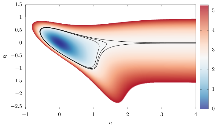
Despite the denominator factors, these expressions are regular at . We show the Ricci scalar curvature in Fig. 2. The curvature for large matches that of the wormhole associated with a single kink and is maximal at (). Because there is a kink and antikink, the metric is doubled and the curvature halved. The potential is shown in Fig. 2; it is asymmetric in and .
IV Effective model dynamics
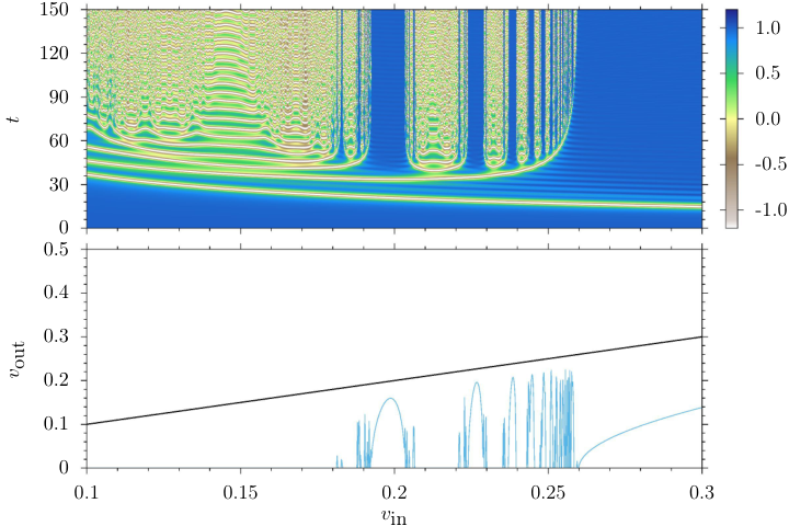
Before discussing KAK collisions in the effective model, let us recall that in the field theory, the main feature is a fractal structure as a function of the initial velocity , distinguishing annihilation to the vacuum and reflection channels, see Fig. 4. The figure shows the time evolution of the field at and the final velocity of the outgoing kink, both as functions of the incoming kink velocity . If the kink and antikink annihilate, is shown as zero. During annihilation, the incoming kink and antikink form a long-lived, quasi-periodic bound state, a bion, which slowly decays by emission of radiation. In the reflection channel, the kink and antikink perform a small number of bounces, then reemerge and separate. The pattern of channels and of particular -bounce windows is fractal. For example, the first 2-bounce window occurs for , and repeats infinitely often as increases. These windows are surrounded by 3-bounce windows, and this picture is replicated for higher-bounce windows. Bion formation occurs in the intermediate velocity intervals, which appear in the figure as bion chimneys.
Overall, the fractal structure occurs in the approximate range – 0.26. For smaller initial velocities there is always bion formation (a wide bion chimney) leading to annihilation, while for larger velocities there is just one bounce before the kink and antikink reflect back to infinity.
We now turn to the effective model (2), defined on the moduli space with coordinates . The dynamical ODEs require appropriate initial conditions. We assume the incoming kink and antikink approach symmetrically and are not vibrating, so impose relation (15) between the initial shape mode amplitude and velocity. The field configuration at each instant is given by (20).
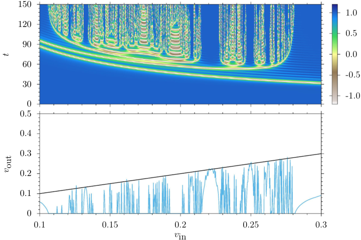
In the effective model, there is similar field evolution and fractal behaviour of velocities as in the field theory, including multi-bounce windows, see Fig. 4. Fractal behaviour now occurs over a wider range of velocities, up to . Because there is no radiation mechanism, the outgoing velocities tend to be larger than in the field theory. Despite this, the velocity patterns match surprisingly well, apart from a small shift . The bion oscillations also match well.
It needs to be stressed that the fractal velocity structure has not previously been reproduced in any effective model derived from the theory KG. Phenomenological models revealing a chaotic behaviour of the positions of the bounce windows and bion chimneys had little to do with the original theory and required arbitrary calibration of couplings.
V Summary
We have investigated an effective, collective coordinate model of symmetric kink-antikink dynamics in theory – a Lagrangian dynamics on a curved 2-dimensional moduli space with a potential, where the coordinates are the KAK separation and the (equal) amplitudes of the KAK shape modes. Two crucial features are: i) initial conditions including excitation of the kink shape modes, modelling Lorentz contractions; ii) regularization of the moduli space metric through use of an improved set of coordinates. There appears to be no problem using a fixed (frozen) shape mode, even though such a mode can disappear into the continuum spectrum as the KAK separation decreases AORW.
The model gives good results for the fractal velocity pattern of KAK scattering, with its multi-bounce windows, and also for the field evolution of bions, where the kink and antikink are captured. It would be desirable to add a dissipation mechanism, modelling the coupling to radiation, to have an upper bound on the number of bounces and for the bion to decay to the vacuum.
Acknowledgements
NSM has been partially supported by the U.K. Science and Technology Facilities Council, consolidated grant ST/P000681/1, and thanks Maciej Dunajski for discussions about wormholes. KO, TR and AW were supported by the Polish National Science Centre, grant NCN 2019/35/B/ST2/00059.
References
- (1) T. Sugiyama, Kink-antikink collisions in the two-dimensional model, Prog. Theor. Phys. 61, 1550 (1979).
- (2) M. Moshir, Soliton-antisoliton scattering and capture in theory, Nucl. Phys. B185, 318 (1981).
- (3) D. K. Campbell, J. F. Schonfeld and C. A. Wingate, Resonance structure in kink-antikink interactions in theory, Physica D9, 1 (1983).
- (4) P. G. Kevrekidis and R. H. Goodman, Four decades of kink interactions in nonlinear Klein-Gordon models: A crucial typo, recent developments and the challenges ahead, https://dsweb.siam.org/The-Magazine/All-Issues/acat/1/archive/102019; [arXiv:1909.03128].
- (5) C. F. S. Pereira, G. Luchini, T. Tassis and C. P. Constantinidis, Some novel considerations about the collective coordinate approximation for the scattering of kinks, J. Phys. A: Math. Theor. 54, 075701 (2021).
- (6) I. Takyi and H. Weigel, Collective coordinates in one-dimensional soliton model revisited, Phys. Rev. D94, 085008 (2016).
- (7) N. S. Manton, K. Oles, T. Romanczukiewicz and A. Wereszczynski, Kink moduli spaces: Collective coordinates reconsidered, Phys. Rev. D103, 025024 (2021).
- (8) N. S. Manton, A remark on the scattering of BPS monopoles, Phys. Lett. B110, 54 (1982).
- (9) M. F. Atiyah and N. J. Hitchin, The Geometry and Dynamics of Magnetic Monopoles, Princeton University Press, Princeton NJ, 1988.
- (10) T. M. Samols, Vortex scattering, Commun. Math. Phys. 145, 149 (1992).
- (11) A. A. Izquierdo, J. Queiroga-Nunes and L. M. Nieto, Scattering between wobbling kinks, Phys. Rev. D103, 045003 (2021).
- (12) C. Adam, K. Oles, T. Romanczukiewicz and A. Wereszczynski, Spectral walls in soliton collisions, Phys. Rev. Lett. 122, 241601 (2019).