Relative Clustering Coefficient
Abstract
In this paper, we relatively extend the definition of global clustering coefficient to another clustering, which we call it relative clustering coefficient. The idea of this definition is to ignore the edges in the network that the probability of having an edge is . Here, we also consider a model as an example that using relative clustering coefficient is better than global clustering coefficient for comparing networks and also checking the properties of the networks.
Keywords: Global clustering coefficient, local clustering coefficient, relative clustering coefficient, networks, graphs
1 Introduction
Recently in the field of physics and statistics, networks and graphs are two interesting topics for example Internet, email, media, and social network, citation network, and so on [9, 1, 6, 7, 8]. One of the properties of graphs is clustering and one of the most important characteristics of networks is that they are highly clustered. It is easy to see that the probability that a person in Germany and a person in Iran make a friendship is so low, but the probability that in a small city in Iran two friends of a person become friends is so high. And this is one of the important characteristics of networks in the real life. In the topological view of the graph, a highly clustered network contains a lot of triangles or cycles of length three. [4]
Networks or graphs [4, 2, 3] contain a set of vertices and a relation between the vertices. The relations between two vertices are defined by edges between the vertices and an edge between two vertices is shown by a line s.t. connects the two vertices. If two vertices have a relation, we add an edge between them otherwise, we do not add any edge between them. If the relationship is one-sided we have a directed graph otherwise, if the relationship is two-sided we have underacted graph. For example, friendship on Facebook is a two-sided relation, therefore if someone sends a request on Facebook to us we both become friends, and we can see what our friends share with us. But, friendship on Instagram is one-sided. When someone sends a friendship request to us, until we do not follow him or her, they will not be our friends. Edges in directed graphs are shown by using a line with an arrow indicating in which direction we have the relationship [4, 2, 3]. Examples of directed and undirected graphs are shown in Figure1.
 |
 | |
| (a) | (b) |
The clustering coefficient was defined by D.J. Watts, and S. H. Strogatz in 1998 [10] and it is used as a measure for comparing networks. We have two definitions for finding the clustering in the graph that we will talk about them in Section 2; global clustering coefficient and local clustering coefficient. Using the definition described in [10], we may define the local clustering coefficient as follows. For an individual , we may consider the neighborhood of as the sub-graph containing only the neighbors of . If this individual is connected to people, then there can exist at most friendships in the neighborhood. The local clustering coefficient for is the number of edges that exist in the neighborhood, divided by , i.e. the proportion of friendships that exist. However, the global clustering coefficient is calculated by the number of triangles divided by the number of triples that could make a triangle. But, after looking and thinking about some networks we see that these clustering coefficients are not sufficient for comparing all the networks and we need to establish and extend the clustering coefficients that we already have read about. And this was the idea of writing this paper.
New work. In this paper, we extend the definition of clustering coefficient to a clustering that can indicate characteristics of networks better and we call it Relative Clustering Coefficient. At this definition, we consider only the edges in the network that we are allowed to add to the network. For example, if two people are in two different prisons they are not connected, although they may have the same lawyer. And if two people are in two different hospitals they are not connected, even though they may have the same doctor who works in those two hospitals.
In this paper, we consider just simple undirected graphs. We will use and talk about some properties of graphs that we illustrate more here. They are bipartite graphs and cliques.
 |
 | |
| (a) | (b) |
Bipartite Graphs [3]:In graph theory, a bipartite graph is a graph that we can divide vertices into two groups of vertices, such that there is no edge between the vertices in each group. (For more illustration look at Figure 2 part ())
Cliques [3]: A complete graph is a simple graph (undirected graph without loops nor multiple edges) that includes all the possible edges between vertices or in other words, there is an edge between any two vertices of the graph. A subset of a graph is a graph that its vertices are the subset of the vertices of the main graph and edges are the subset of the edges of the main graph that connects vertices of the sub-graph. A clique is a sub-graph of a graph that is complete. (For more illustration look at Figure 2 part ())
Here the outline of this paper is as follows: in Section 2 we present the definition of clustering coefficients that we already had; global clustering coefficient and local clustering coefficient. We extend the definition of clustering coefficient at Section 3. We also present an example of a model and we use relative clustering coefficient instead of clustering coefficient. Last section which is Section 4 is conclusion.
2 Clustering Coefficient
If we consider different networks in the real life we see that most of them are highly clustered, i.e. we can see that a friend of a friend of a person is a friend of the person as well. In another word, two friends of a person are with high probability friends in a way. From the topological view, we can see that there are lots of triangles in a network [7, 10]. There are two definitions to measure the clustering in the network; local clustering coefficient and global clustering coefficient. Here we want to illustrate these two definitions.
2.1 Local Clustering Coefficient
As it is defined in [10], the local clustering coefficient for a vertex in a graph is defined as the number of triangles in the graph such that one vertex of the triangle is divided by the number of paths in with the length of such that the vertex is the middle vertex of .
In other words, for an undirected graph, if we consider as a set of vertices in the neighborhood of a vertex , that means the set of vertices that there is an edge between and every vertex in the set, so we have that
Therefore, for a vertex we can define the local clustering coefficient as the number of edges between vertices in the set of divided by the number of edges that can exist between the vertices in the set .
Therefore, we can define the local clustering coefficient for a vertex as follows:
Definition 1.
[7] Local Clustering Coefficient
For a vertex , if is the set of vertices in the neighbourhood of and is the size of this set, the local clustering for the vertex is defined as follows:
We can define the local clustering coefficient for a directed graph in a similar way, but it is beyond the scope of this paper.
2.2 Global Clustering Coefficient
If we consider as the number of triangles in the graph and as the number of sub-graphs containing three vertices that are connected at least by two edges (It means there is two edges between them or three edges, look at the Figure 3), the definition of clustering in a graph or network is as follows:
 |
 |
 | ||
| (a) | (b) | (c) |
Definition 2.
[7] Global Clustering Coefficient
By using the notations and that we defined earlier, the global Clustering Coefficient is defined as follows:
After looking and considering other examples of networks we see that these definitions are not sufficient for considering high clustering in the network, so we define relative clustering coefficient. We consider the next section to illustrate and talk about the relative clustering coefficient. Later we give an example that we see that considering the global clustering coefficient is not good enough.
3 Relative Clustering Coefficient (RCC)
The idea of the definition of RCC is as follows that we just consider pairs of vertices that we can have an edge between them in the network. In other words, the probability of having an edge between them is larger than . Here, for each pair of vertices, we define a capacity (a number, or ). If we can have an edge between two vertices (Or if the probability of having an edge between two vertices is larger than ) the capacity is , otherwise, the capacity is . is the number of all the triangles in the network that all the edges in the triangles have a capacity of , and is the number of triangles that the capacity of all the edges in it is , such that all the edges in the triangle are in the network, and is the number of triangles that the capacity of all edges in it is , but just two of the edges in the triangle are in the network. Now, we define the relative clustering coefficient in a network as follows:
Definition 3.
Relative Clustering Coefficient
By using the notation that we have illustrated earlier, we defined RCC as follows:
Example 1.
If we consider a group of people ( and ) in hospital number and two other people ( and ) that are hospitalized in hospital number , and the person a doctor that works with patients in both hospitals (For more information look at Figure 4) we have RCC and CC as follows:
while
But, in this case, we cannot add any edge to this network, because these two groups of people are separated and there is no physical contact between them. Therefore, the clustering coefficient should be .
 |
 | |
| (a) | (b) |
3.1 RCC instead of CC
In [7] M. E. J. Newman illustrated a model for highly clustered networks. The model is as follows:
Model 1.
[7]
We have individuals in total
These individuals are divided into different groups.
Individuals can belong to more than one group
Individuals belong to groups randomly
If two individuals belong to one group with the probability of they are connected otherwise they are not connected.
To illustrate this model better, we use an example:
Example 2.
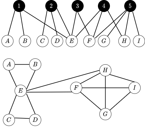
We have some professors A,B,C,D,E,F,G,H,I who work at the University of Tehran. At the University of Tehran, we have some different departments (, , , , ) that each professor belongs to. Some professors work in different departments. Therefore, in meetings that are held in different departments that they participate in, they can meet other professors in the department. But, two professors who do not work in the same department, do not have any information from each other. (For more information look at Figure 5)
Definition 4.
Full Graph
If we construct a network that contains all the edges with the probability of , we have a graph that we call it full graph. (See the lower figure in Figure 5)
For this model, M. E. J. Newman used the clustering coefficient and showed that
such that is the clustering of the full graph of the network.
Reason for using RCC.
Here, if we look at the full graph, we cannot add any edge to the network, so it is better if we use RCC instead of CC. Because it (the full graph) has all the edges between any pair of vertices and we are not allowed to add any other edges to the full graph.
Therefore, by using RCC we have the following theorem which is more reasonable to use for this example and model.
Theorem 1.
For the Model 1 for large , where is the number of vertex in the network, we have that
which is the probability of having an edge between two vertices in the network.
Proof.
For each of the cliques of size three (that also have capacity for each edge), we define as the number of edges within clique number . The number of given one of this cliques in binomially distributed with three numbers of trials and probability of success p, therefore .
The probability of all three edges existing within one of these cliques is
while the probability of exactly two edges existing with one of these cliques is
We define indicator variables as follows:
Therefore, these indicator variables will have Bernolli distributions and expectations, so we have:
Therefore, for large enough the following relative clustering coefficient will asymptotcally go towards
∎
We can use a similar definition for defining relative local clustering coefficient as well.
Definition 5.
[5] For two functions and we say that , if there exist two constant numbers and and an integer numbers such that for all , we can write:
4 Conclusion
In this paper, we extend the definition of clustering coefficient to another definition which we called it relative clustering coefficient. This coefficient can measure the properties of networks better. In section 2 we defined two clustering coefficients, one local clustering, and another global clustering coefficient. We extended the definition of clustering coefficient in section 3 and we used the clustering for measuring the property of a model as an example.
References
- [1] Réka Albert and Albert-László Barabási. Statistical mechanics of complex networks. Reviews of Modern Physics, 74(1):47–97, January 2002.
- [2] Béla Bollobás. Modern Graph Theory. Graduate Texts in Mathematics 184. Springer-Verlag New York, 1 edition, 1998.
- [3] J. A. Bondy and U. S. R. Murty. Graph Theory with Applications. Elsevier, New York, 1976.
- [4] Caldarelli, G., Pastor-Satorras, R., and Vespignani, A. Structure of cycles and local ordering in complex networks. Eur. Phys. J. B, 38(2):183–186, 2004.
- [5] Thomas H. Cormen, Charles E. Leiserson, Ronald L. Rivest, and Clifford Stein. Introduction to Algorithms. The MIT Press, 2nd edition, 2001.
- [6] S. N. Dorogovtsev and J. F. F. Mendes. Evolution of networks with aging of sites. Physical Review E, 62(2):1842–1845, Aug 2000.
- [7] M. E. J. Newman. Properties of highly clustered networks. Phys. Rev. E, 68:026121, Aug 2003.
- [8] M. E. J. Newman, S. H. Strogatz, and D. J. Watts. Random graphs with arbitrary degree distributions and their applications. Phys. Rev. E, 64(2):026118, July 2001.
- [9] Steven H. Strogatz. Exploring complex networks. Nature, 410(6825):268–276, March 2001.
- [10] Duncan J. Watts and Steven H. Strogatz. Collective dynamics of ‘small-world’ networks. Nature, 393(6684):440–442, 1998.