Contamination Bias in Linear RegressionsThanks: Contact: paul.goldsmith-pinkham@yale.edu, peter_hull@brown.edu, and mkolesar@princeton.edu. We thank Alberto Abadie, Jason Abaluck, Isaiah Andrews, Josh Angrist, Tim Armstrong, Kirill Borusyak, Kyle Butts, Clément de Chaisemartin, Peng Ding, Len Goff, Jin Hahn, Xavier D’Haultfœuille, Simon Lee, Bernard Salanié, Pedro Sant’Anna, Tymon Słoczyński, Isaac Sorkin, Jonathan Roth, Jacob Wallace, Stefan Wager, and numerous seminar participants for helpful comments. Hull acknowledges support from National Science Foundation Grant SES-2049250. Kolesár acknowledges support by the Sloan Research Fellowship and by the National Science Foundation Grant SES-22049356. Mauricio Cáceres Bravo, Jerray Chang, William Cox, and Dwaipayan Saha provided expert research assistance. An earlier draft of this paper circulated under the title “On Estimating Multiple Treatment Effects with Regression.”

Consider the regression of an outcome $Y_{i}$ on a single treatment indicator $D_{i}\in\{0,1\}$, a single binary control $W_{i}\in\{0,1\}$, and an intercept:

By definition, $U_{i}$ is a mean-zero regression residual that is uncorrelated with $D_{i}$ and $W_{i}$. For example, analysing the Project STAR trial, Krueger 1999a primarily studied the effect of small class size $D_{i}$ on the test scores $Y_{i}$ of kindergartners indexed by $i$. Project STAR randomized students to classes within schools, with the fraction of students assigned to small classes varying by school due to the varying number of total students in each school. To account for this, Krueger 1999a included school fixed effects as controls. Such specifications are often found in stratified RCT with varying treatment assignment rates across a set of pre-treatment strata. If we imagine two such strata, demarcated by a binary indicator $W_{i}$, then eq. 1 corresponds to a stylized two-school version of a Project STAR regression.

We wish to interpret the coefficient $\beta$ in terms of the causal effects of $D_{i}$ on $Y_{i}$. For this we use potential outcome notation, letting $Y_{i}(d)$ denote the test score of student $i$ when $D_{i}=d$. Individual $i$’s treatment effect is then given by $\tau_{1i}=Y_{i}(1)-Y_{i}(0)$, and we can write realized achievement as $Y_{i}=Y_{i}(0)+\tau_{1i}D_{i}$. Since treatment assignment is random within schools, $D_{i}$ is conditionally independent of potential outcomes given $W_{i}$: $\left(Y_{i}(0),Y_{i}(1)\right)\perp D_{i}\mid W_{i}$.

Angrist 1998a showed that regression coefficients like $\beta$ identify a convexly-weighted average of within-strata ATE. In our Project STAR example, this result shows that:

gives a convex weighting scheme, and $\tau_{1}(w)=E[Y_{i}(1)-Y_{i}(0)\mid W_{i}=w]$ is the ATE in school $w\in\{0,1\}$. Thus, in our example the coefficient $\beta$ identifies a weighted average of school-specific small classroom effects $\tau_{1}(w)$ across the two schools.

Equation 2 can be derived by applying the FWL (FWL) Theorem. The multivariate regression coefficient $\beta$ can be written as a univariate regression coefficient from regressing $Y_{i}$ onto the population residual $\tilde{D}_{i}$ from regressing $D_{i}$ onto $W_{i}$ and a constant:

where we substitute the potential outcome model for $Y_{i}$ in the second equality. Since $W_{i}$ is binary, the propensity score $E[D_{i}\mid W_{i}]$ is linear and the residual $\tilde{D_{i}}$ is mean independent of $W_{i}$ (not just uncorrelated with it): $E[\tilde{D_{i}}\mid W_{i}]=0$. Therefore,

The first equality in eq. 4 follows from the law of iterated expectations, the second equality follows by the conditional random assignment of $D_{i}$ and the third equality uses $E[\tilde{D_{i}}\mid W_{i}]=0$. Hence, the first summand in eq. 3 is zero. Analogous arguments show that

where $\var(D_{i}\mid W_{i})=E[\tilde{D}_{i}^{2}\mid W_{i}]$ gives the conditional variance of the small-class treatment within schools. Since $E[\var(D_{i}\mid W_{i})]=E[E[\tilde{D}_{i}^{2}\mid W_{i}]]=E[\tilde{D}_{i}^{2}]$, it follows that we can write the second summand in eq. 3 as

proving the representation of $\beta$ in eq. 2.

The key fact underlying this derivation is that the residual $\tilde{D}_{i}$ from the auxiliary regression of the treatment $D_{i}$ on the other regressors $W_{i}$ is mean-independent of $W_{i}$. By the FWL theorem, treatment coefficients like $\beta$ can always be represented as in eq. 3 even without this property. We next show, however, that the remaining steps in the derivation of eq. 2 fail when an additional treatment arm is included. This failure can be attributed to the fact that the auxiliary FWL regression delivers a treatment residual that is uncorrelated with—but not mean-independent of—the other regressors. The lack of mean independence leads to an additional term in the expression for the regression coefficient.

In reality, Project STAR randomized students to three mutually exclusive conditions within schools: a control group with a regular class ($D_{i}=0$), a treatment that reduced class size ($D_{i}=1$), and a treatment that introduced full-time teaching aides ($D_{i}=2$). We incorporate this extension of our stylized example by considering a regression of student achievement $Y_{i}$ on a vector of two treatment indicators, $X_{i}=(X_{i1},X_{i2})^{\prime}$, where $X_{ik}=\operatorname{\mathbbm{1}}\{D_{i}=k\}$ indicates assignment to treatment $k=1,2$. We continue to include a constant and the school indicator $W_{i}$ as controls, yielding the regression

The observed outcome is now given by $Y_{i}=Y_{i}(0)+\tau_{i1}X_{i1}+\tau_{i2}X_{i2}$, with $\tau_{i1}=Y_{i}(1)-Y_{i}(0)$ and $\tau_{i2}=Y_{i}(2)-Y_{i}(0)$ denoting the potentially heterogeneous effects of a class size reduction and introduction of a teaching aide, respectively. As before, we analyze this regression by assuming ${X}_{i}$ is conditionally independent of the potential achievement outcomes $Y_{i}(d)$ given the school indicator $W_{i}$: $\left(Y_{i}(0),Y_{i}(1),Y_{i}(2)\right)\perp{X}_{i}\mid W_{i}$.

To analyze the coefficient on $X_{i1}$, we again use the FWL theorem to write

where $\accentset{\approx}{X}_{i1}$ again denotes a population residual, but now from regressing $X_{i1}$ on $W_{i}$, a constant, and $X_{i2}$. Unlike before, this residual is uncorrelated with but not mean-independent of the remaining regressors $(W_{i},X_{i2})$ because the dependence between $X_{i1}$ and $X_{i2}$ is non-linear. When $X_{i2}=1$, $X_{i1}$ must be zero regardless of the value of $W_{i}$ (because they are mutually exclusive) while if $X_{i2}=0$ the mean of $X_{i1}$ does depend on $W_{i}$ unless the treatment assignment is completely random. Thus, in general, $\accentset{\approx}{X}_{i1}\neq X_{i1}-E[X_{i1}\mid W_{i},X_{i2}]$.

Because $\accentset{\approx}{X}_{i1}$ does not coincide with a conditionally de-meaned $X_{i1}$, we can not generally reduce eq. 6 to an expression involving only the effects of the first treatment arm, $\tau_{i1}$. It turns out that we nevertheless still have $E[\accentset{\approx}{X}_{i1}Y_{i}(0)]=0$, as in eq. 4, since the auxilliary regression residuals are still uncorrelated with any individual characteristic like $Y_{i}(0)$.⁸⁸ 8 To see this, note that in the auxiliary regression $X_{i1}=\mu_{0}+\mu_{1}X_{i2}+\mu_{2}W_{i}+\accentset{\approx}{X}_{i1}$ we can partial out $W_{i}$ and the constant from both sides to write $\tilde{X}_{i1}=\mu_{1}\tilde{X}_{i2}+\accentset{\approx}{X}_{i1}$. Thus, $\accentset{\approx}{X}_{i1}=\tilde{X}_{i1}-\mu_{1}\tilde{X}_{i2}$ is a linear combination of residuals which, per eq. 4, are both uncorrelated with $Y_{i}(0)$. It follows that $E[\accentset{\approx}{X}_{i1}Y_{i}(0)]=0$. The regression thus does not suffer from OVB. However, we do not generally have $E[\accentset{\approx}{X}_{i1}X_{i2}\tau_{i2}]=0$. Instead, simplifying eq. 6 by the same steps as before leads to the expression

as a generalization of eq. 2. Here $\lambda_{11}(W_{i})=E[\accentset{\approx}{X}_{i1}X_{i1}\mid W_{i}]/E[\accentset{\approx}{X}_{i1}^{2}]$ can be shown to be non-negative and to average to one, similar to the $\phi$ weight in eq. 2. Thus, if not for the second term in eq. 7, $\beta_{1}$ would similarly identify a convex average of the conditional ATE $\tau_{1}(W_{i})=E[Y_{i}(1)-Y_{i}(0)\mid W_{i}]$. But precisely because $\accentset{\approx}{X}_{i1}\neq X_{i1}-E[X_{i1}\mid W_{i},X_{i2}]$, this second term is generally present: $\lambda_{12}(W_{i})=E[\accentset{\approx}{X}_{i1}X_{i2}\mid W_{i}]/E[\accentset{\approx}{X}_{i1}^{2}]$ is generally non-zero, complicating the interpretation of $\beta_{1}$ by including the conditional effects of the other treatment $\tau_{2}(W_{i})=E[Y_{i}(2)-Y_{i}(0)\mid W_{i}]$.

The second contamination bias term in eq. 7 arises because the residualized small class treatment $\accentset{\approx}{X}_{i1}$ is not conditionally independent of the second full-time aide treatment $X_{i2}$ within schools, despite being uncorrelated with $X_{i2}$ by construction. This can be seen by viewing $\accentset{\approx}{X}_{i1}$ as the result of an equivalent two-step residualization. First, both $X_{i1}$ and $X_{i2}$ are de-meaned within schools: $\tilde{X}_{i1}=X_{i1}-E[X_{i1}\mid W_{i}]=X_{i1}-p_{1}(W_{i})$ and $\tilde{X}_{i2}=X_{i2}-E[X_{i2}\mid W_{i}]=X_{i2}-p_{2}(W_{i})$ where $p_{j}(W_{i})=E[X_{ij}\mid W_{i}]$ gives the propensity score for treatment $j$. Second, a bivariate regression of $\tilde{X}_{i1}$ on $\tilde{X}_{i2}$ is used to generate the residuals $\accentset{\approx}{X}_{i1}$. When the propensity scores vary across the schools (i.e. $p_{j}(0)\neq p_{j}(1)$), the relationship between these residuals varies by school, and the line of best fit between $\tilde{X}_{i1}$ and $\tilde{X}_{i2}$ averages across this relationship. As a result, the line of best fit does not isolate the conditional (i.e. within-school) variation in $X_{i1}$: the remaining variation in $\accentset{\approx}{X}_{i1}$ will tend to predict $X_{i2}$ within schools, making the contamination weight $\lambda_{12}(W_{i})$ non-zero.

A simple numerical example helps make the contamination bias problem concrete. Suppose in the previous setting that school $0$ (indicated by $W_{i}=0$) assigned only 5 percent of the students to the small classroom treatment, with 45 percent of the students assigned to the full-time aide treatment and the rest assigned to the control group. In school $1$ (indicated by $W_{i}=1$), there was a substantially larger push for students to be placed into treatment groups with 45 percent of students assigned to a small classroom, 45 percent assigned to a classroom with a full-time aide, and only 10 percent assigned to the control group. Therefore, $p_{1}(0)=0.05$ and $p_{2}(0)=0.45$ while $p_{1}(1)=p_{2}(1)=0.45$. Suppose that the schools have the same number of students, so that $\Pr(W_{i}=1)=0.5$. It then follows from the above formulas that $\lambda_{12}(0)=99/106$ and $\lambda_{12}(1)=-99/106$.

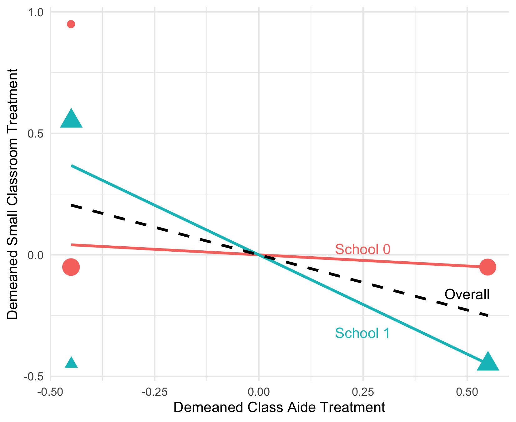
As reasoned above, the contamination weights are non-zero here because the within-school correlation between the residualized treatments, $\tilde{X}_{i1}$ and $\tilde{X}_{i12}$, is heterogeneous: in school $0$ it is about $-0.2$, so that the value of the demeaned class aide treatment is only weakly predictive of the small classroom treatment, while in school $1$ it is highly predictive with correlation $-0.8$. Figure D.1 in Appendix D illustrates this graphically, showing that because the overall regression of $\tilde{X}_{i1}$ on $\tilde{X}_{i2}$ averages over these two correlations, the regression residuals are predictive of the value of the class aide treatment.

To illustrate the potential magnitude of bias in this example, suppose that classroom reductions have no effect on student achievement (so $\tau_{1}(0)=\tau_{1}(1)=0$), but that the effect of a teaching aide varies across schools. In school $1$ the aide is highly effective, $\tau_{2}(1)=1$, (which may be the reason for the higher push in this school to place students into treatment groups) but in school $0$, the aide has no effect, $\tau_{2}(0)=0$. By eq. 7, the regression coefficient on the first treatment identifies

Thus, in this example, a researcher would conclude that small classrooms have a sizable negative effect on student achievement—equal in magnitude to around half of the true teaching aide effect in school $1$—despite the true small-classroom effect being zero for all students. This treatment effect coefficient can be engineered to match an arbitrary magnitude and sign by varying the heterogeneity of the teaching aide effects across schools.

To build further intuition for eq. 7, it is useful to consider two cases where the contamination bias term is zero. First, note that since regression residuals are by construction uncorrelated with the included regressors, $E[\lambda_{12}(W_{i})]=E[\accentset{\approx}{X}_{i1}X_{i2}]/E[\accentset{\approx}{X}_{i1}^{2}]=0$. Therefore, $E[\lambda_{12}(W_{i})\tau_{2}(W_{i})]=E[\lambda_{12}(W_{i})\tau_{2}(W_{i})]-E[\lambda_{12}(W_{i})]E[\tau_{2}(W_{i})]=\cov(\lambda_{12}(W_{i}),\tau_{2}(W_{i}))$. If the average effects of the teaching aide treatment are constant across the two schools, $\tau_{2}(1)=\tau_{2}(0)$, then $\tau_{2}(W_{i})$ is constant, and this covariance is zero such that contamination bias disappears. More generally, when the average teaching aide treatment effects across schools $\tau_{2}(W_{i})$ exhibit idiosyncratic variation, in the sense that they have a weak covariance with the contamination weights across schools, the contamination bias term will be small.

Second, consider the case where $X_{i1}$ and $X_{i2}$ are independent conditional on $W_{i}$—such as when the small classroom and teacher aid interventions are independently assigned within schools, in contrast to the previously assumed mutual exclusivity of these treatments. In this case the conditional expectation $E[X_{i1}\mid W_{i},X_{i2}]=E[X_{i1}\mid W_{i}]$ will be linear, since $X_{i1}$ and $X_{i2}$ are unrelated given $W_{i}$, and will thus be identified by the auxiliary regression of $X_{i1}$ on $W_{i}$, $X_{i2}$, and a constant. Consequently, the $\accentset{\approx}{X}_{i1}$ residuals will coincide with $X_{i1}-E[X_{i1}\mid W_{i}]$. The coefficient on $X_{i1}$ in eq. 5 can therefore be shown to be equivalent to the previous eq. 2, identifying the same convex average of $\tau_{1}(w)$. This case highlights that dependence across treatments is necessary for the contamination bias to arise.

We now consider the interpretation of each treatment coefficient $\beta_{k}$ in terms of causal effects. Let $Y_{i}(k)$ denote the potential outcome of unit $i$ when $D_{i}=k$. Observed outcomes are given by $Y_{i}=Y_{i}(D_{i})=Y_{i}(0)+X_{i}^{\prime}\tau_{i}$ where $\tau_{i}$ is a vector of treatment effects with elements $\tau_{ik}=Y_{i}(k)-Y_{i}(0)$. We denote the conditional expectation of the vector of treatment effects given the controls by $\tau(W_{i})=E[\tau_{i}\mid W_{i}]$, so that $\tau_{k}(W_{i})$ is the conditional ATE for the $k$th treatment. We let $p(W_{i})=E[X_{i}\mid W_{i}]$ denote the vector of propensity scores, so that $p_{k}(W_{i})=\Pr(D_{i}=k\mid W_{i})$. Our characterization of contamination bias doesn’t require the propensity scores to be bounded away from $0$ and $1$ and in fact allows them to be degenerate, i.e. $p_{k}(w)\in\{0,1\}$ for all $w$. This is the case in Example 2, since $X_{i}$ is a non-random function of $W_{i}$. We return to practical questions of propensity score support in Section 4.

We make two assumptions to interpret $\beta_{k}$ in terms of the effects $\tau_{i}$. First, we assume mean-independence of the potential outcomes and treatment, conditional on the controls:

Second, we assume $\mathcal{G}$ is specified such that that one of two conditions holds:

In Example 2, with $X_{i}$ being a deterministic function of unit and time indices and $g(W_{i})$ including unit and time fixed effects, eq. 12 fails because the propensity scores are binary—they cannot be captured by a linear combination of the TWFE. However, eq. 13 is satisfied by a parallel trends assumption: that the average untreated potential outcomes $Y_{i}(0)$ are linear in the unit and time effects. We elaborate on this setup in Appendix B.¹⁰¹⁰ 10 Identification based on eq. 12 can be seen as “design-based” in that it only restricts the treatment assignment process. Identification based on eq. 13 can be seen as “model-based” in that it makes no assumptions on the treatment assignment process but specifies a model for the unobserved untreated potential outcomes.

Under either condition in 2, the specification of controls is flexible enough to avoid OVB. To see this formally, suppose all treatment effects are constant: $\tau_{ik}=\tau_{k}$ for all $k$. This restriction lets us write $Y_{i}=Y_{i}(0)+X_{i}^{\prime}\tau$, where $\tau$ is a vector collecting the constant effects. The only source of bias when regressing $Y_{i}$ on $X_{i}$ and controls is then the unobserved variation in the untreated potential outcomes $Y_{i}(0)$. But it follows from the expression for $\beta$ in eq. 10 that there is no such OVB when 2 holds:

Here the first equality uses the fact that $E[\tilde{{X}}_{i}X_{i}^{\prime}]=E[\tilde{X}_{i}\tilde{X}_{i}^{\prime}]$ because $\tilde{X}_{i}$ is a vector of projection residuals, and the second equality uses the law of iterated expectations and 1. Under eq. 12, $E[\tilde{X}_{i}\mid W_{i}]=0$, so that the term in braces is zero by another application of the law of iterated expectations: $E[\tilde{X}_{i}E[Y_{i}(0)\mid W_{i}]]=E[E[\tilde{X}_{i}\mid W_{i}]E[Y_{i}(0)\mid W_{i}]]=0$. It is likewise zero under eq. 13 since $\tilde{X}_{i}$ is by definition of projection orthogonal to any function in $\mathcal{G}$ such that $E[\tilde{X}_{i}E[Y_{i}(0)\mid W_{i}]]=E[\tilde{X}_{i}\mu_{0}(W_{i})]=0$. Hence, OVB is avoided in the constant-effects case so long as either the propensity scores or the untreated potential outcomes are spanned by the control specification. Versions of this double robustness property have been previously observed in, for instance, Robins et al. 1992a.

When treatment effects are heterogeneous but ${X}_{i}$ contains a single treatment indicator, $\beta$ identifies a weighted average of the conditional effects $\tau(W_{i})$. Specifically, since by the previous argument we still have $E[\tilde{X}_{i}Y_{i}(0)]=0$, it follows from eq. 10 that

where the second equality uses iterated expectations and the identity $E[\tilde{{X}}_{i}^{2}]=E[\tilde{X}_{i}{X}_{i}]$. Under eq. 12, $E[\tilde{X}_{i}X_{i}\mid W_{i}]=E[\tilde{X}_{i}^{2}\mid W_{i}]=\var(X_{i}\mid W_{i})$, so the weights further simplify to $\lambda_{11}(W_{i})=\frac{\var(X_{i}\mid W_{i})}{E[\var(X_{i}\mid W_{i})]}\geq 0$. This extends the Angrist 1998a result to a general control specification; versions of this extension appear in, for instance, Angrist & Krueger 1999a, Angrist & Pischke 2009a, and Aronow & Samii 2016a.

This result provides a robustness rationale for estimating the effect of a single as-good-as-randomly assigned treatment with a partially linear model (8): so long as the specification of $\mathcal{G}$ is rich enough to make eq. 12 hold, $\beta$ will identify a convex average of heterogeneous treatment effects. In Section 4 we will derive another rationale for targeting $\beta$ in this model, showing that the weights $\lambda_{11}(W_{i})$ minimize the semiparametric efficiency bound (conditional on the controls) for estimating some weighted-average treatment effect.

Our first proposition shows that with multiple treatments, the interpretation of $\beta$ becomes more complicated because of contamination bias:

Hence, if the linear probability model is correctly specified, i.e. $E[X_{ik}\mid{X}_{i,-k},W_{i}]=X_{i,-k}^{\prime}\alpha+g_{k}(W_{i})$ for some vector $\alpha$ and $g_{k}\in\mathcal{G}$, the contamination weights $\lambda_{k\ell}(W_{i})$ are zero and the own treatment weights $\lambda_{kk}(W_{i})$ are positive. This is the analog of condition (12) if we interpret $X_{ik}$ as a binary treatment of interest and $X_{i,-k}^{\prime}\alpha+g_{k}(W_{i})$ as a specification for the controls. In other words, the assignment of treatment $k$ must be additively separable between $X_{i,-k}$ and $W_{i}$. However, with mutually exclusive treatments, this won’t be the case unless treatment assignment is unconditionally random. In particular, since $X_{ik}$ must equal zero if the unit is assigned to one of the other treatments regardless of the value of $W_{i}$, under correct specification it must be the case that $\alpha_{\ell}=-g_{k}(W_{i})$ for all elements $\alpha_{\ell}$ of $\alpha$. This in turn implies that the assignment of treatment $k$ doesn’t depend on $W_{i}$, which is impossible unless the propensity score $p_{k}(W_{i})$ is constant.

Thus, misspecification in the linear probability model will generally yield nonsensical fitted probabilities $E^{*}[X_{ik}\mid X_{i\ell}=1,W_{i}]\neq 0$ that generate non-zero contamination weights $\lambda_{k\ell}(W_{i})$. Furthermore, if the misspecification also yields fitted probabilities $E^{*}[X_{ik}\mid X_{i,-k}=0,W_{i}]>1$, we will have negative own treatment weights. The last part of Proposition 1 shows that such nonsensible predictions are ruled out if eq. 12 holds.

We make four further remarks on our general characterization of contamination bias:

References

- Abadie & Cattaneo (2018) Alberto Abadie and Matias. Cattaneo “Econometric Methods for Program Evaluation” In Annual Review of Economics 10.1, 2018, pp. 465–503 DOI: 10.1146/annurev-economics-080217-053402
- Abadie et al. (2020) Alberto Abadie et al. “Sampling-Based versus Design-Based Uncertainty in Regression Analysis” In Econometrica 88.1, 2020, pp. 265–296 DOI: 10.3982/ECTA12675
- Abaluck et al. (2021) Jason Abaluck et al. “Mortality effects and choice across private health insurance plans” In The Quarterly Journal of Economics 136.3, 2021, pp. 1557–1610 DOI: 10.1093/qje/qjab017
- Angrist et al. (2024) Joshua Angrist et al. “Credible School Value-Added with Undersubscribed School Lotteries” In Review of Economics and Statistics 106.1, 2024, pp. 1–19 DOI: 10.1162/rest_a_01149
- Angrist (1998) Joshua. Angrist “Estimating the Labor Market Impact of Voluntary Military Service Using Social Security Data on Military Applicants” In Econometrica 66.2, 1998, pp. 249–288 DOI: 10.2307/2998558
- Angrist & Krueger (1999) Joshua. Angrist and Alan. Krueger “Empirical Strategies in Labor Economics” In Handbook of Labor Economics 3A Amsterdam: Elsevier, 1999, pp. 1277–1366 DOI: 10.1016/S1573-4463(99)03004-7
- Angrist & Pischke (2009) Joshua. Angrist and Jorn-Steffen Pischke “Mostly Harmless Econometrics: An Empiricist’s Companion” Princeton, NJ: Princeton University Press, 2009 DOI: 10.2307/j.ctvcm4j72
- Angrist et al. (1999) Joshua. Angrist, Guido. Imbens and Alan. Krueger “Jackknife Instrumental Variables Estimation” In Journal of Applied Econometrics 14.1, 1999, pp. 57–67 DOI: 10.1002/(SICI)1099-1255(199901/02)14:1<57::AID-JAE501>3.0.CO;2-G
- Angrist et al. (2017) Joshua. Angrist et al. “Leveraging lotteries for school value-added: Testing and estimation” In The Quarterly Journal of Economics 132.2, 2017, pp. 871–919 DOI: 10.1093/qje/qjx001
- Aronow & Samii (2016) Peter. Aronow and Cyrus Samii “Does Regression Produce Representative Estimates of Causal Effects?” In American Journal of Political Science 60.1, 2016, pp. 250–267 DOI: 10.1111/ajps.12185
- Athey & Imbens (2022) Susan Athey and Guido. Imbens “Design-based analysis in difference-in-differences settings with staggered adoption” In Journal of Econometrics 226.1, 2022, pp. 62–79 DOI: 10.1016/j.jeconom.2020.10.012
- Behaghel et al. (2013) Luc Behaghel, Bruno Crépon and Marc Gurgand “Robustness of the encouragement design in a two-treatment randomized control trial”, 2013
- Benhassine et al. (2015) Najy Benhassine et al. “Turning a Shove into a Nudge? A “Labeled Cash Transfer” for Education” In American Economic Journal: Economic Policy 7.3, 2015, pp. 86–125 DOI: 10.1257/pol.20130225
- Berman & Plemmons (1994) Abraham Berman and Robert. Plemmons “Nonnegative Matrices in the Mathematical Sciences”, Classics in Applied Mathematics 9 Philadelphia, PA: Society for Industrial and Applied Mathematics, 1994 DOI: 10.1137/1.9781611971262
- Bhuller & Sigstad (2024) Manudeep Bhuller and Henrik Sigstad “2SLS with Multiple Treatments” In Journal of Econometrics 242.1, 2024, pp. 105785 DOI: 10.1016/j.jeconom.2024.105785
- Blandhol et al. (2022) Christine Blandhol et al. “When is TSLS Actually LATE?”, 2022 DOI: 10.2139/ssrn.4014707
- Borusyak et al. (2024) Kirill Borusyak, Xavier Jaravel and Jann Spiess “Revisiting Event-Study Designs: Robust and Efficient Estimation” In Review of Economic Studies, 2024 DOI: 10.1093/restud/rdae007
- Callaway & Sant’Anna (2021) Brantly Callaway and Pedro.C. Sant’Anna “Difference-in-differences with multiple time periods” In Journal of Econometrics 225.2, 2021, pp. 200–230 DOI: 10.1016/j.jeconom.2020.12.001
- Cattaneo (2010) Matias. Cattaneo “Efficient Semiparametric Estimation of Multi-Valued Treatment Effects under Ignorability” In Journal of Econometrics 155.2, 2010, pp. 138–154 DOI: 10.1016/j.jeconom.2009.09.023
- Chattopadhyay & Zubizarreta (2021) Ambarish Chattopadhyay and Jose. Zubizarreta “On the Implied Weights of Linear Regression for Causal Inference”, 2021 arXiv:2104.06581v2
- Chen et al. (2008) Xiaohong Chen, Han Hong and Alessandro Tarozzi “Semiparametric Efficiency in GMM Models with Auxiliary Data” In The Annals of Statistics 36.2, 2008, pp. 808–843 DOI: 10.1214/009053607000000947
- Chernozhukov et al. (2022) Victor Chernozhukov et al. “Locally Robust Semiparametric Estimation” In Econometrica 90.4, 2022, pp. 1501–1535 DOI: 10.3982/ECTA16294
- Chernozhukov et al. (2022a) Victor Chernozhukov, Whitney. Newey and Rahul Singh “Automatic Debiased Machine Learning of Causal and Structural Effects” In Econometrica 90.3, 2022, pp. 967–1027 DOI: 10.3982/ECTA18515
- Chernozhukov et al. (2018) Victor Chernozhukov et al. “Double/Debiased Machine Learning for Treatment and Structural Parameters” In The Econometrics Journal 21.1, 2018, pp. C1–C68 DOI: 10.1111/ectj.12097
- Chetty et al. (2014) Raj Chetty, John. Friedman and Jonah. Rockoff “Measuring the impacts of teachers I: Evaluating bias in teacher value-added estimates” In American Economic Review 104.9, 2014, pp. 2593–2632 DOI: 10.1257/aer.104.9.2593
- Cole et al. (2013) Shawn Cole et al. “Barriers to Household Risk Management: Evidence from India” In American Economic Journal: Applied Economics 5.1, 2013, pp. 104–135 DOI: 10.1257/app.5.1.104
- Crump et al. (2006) Richard. Crump et al. “Moving the Goalposts: Addressing Limited Overlap in the Estimation of Average Treatment Effects by Changing the Estimand”, 2006 DOI: 10.3386/t0330
- Crump et al. (2009) Richard. Crump et al. “Dealing with limited overlap in estimation of average treatment effects” In Biometrika 96.1, 2009, pp. 187–199 DOI: 10.1093/biomet/asn055
- De & D’Haultfœuille (2023) Clément De and Xavier D’Haultfœuille “Two-Way Fixed Effects and Differences-in-Differences Estimators with Several Treatments” In Journal of Econometrics 236.2, 2023, pp. 105480 DOI: 10.1016/j.jeconom.2023.105480
- de Chaisemartin & D’Haultfœuille (2020) Clément de Chaisemartin and Xavier D’Haultfœuille “Two-Way Fixed Effects Estimators with Heterogeneous Treatment Effects” In American Economic Review 110.9, 2020, pp. 2964–2996 DOI: 10.1257/aer.20181169
- de los Angeles Resa & Zubizarreta (2020) María de los Angeles Resa and José. Zubizarreta “Direct and Stable Weight Adjustment in Non-Experimental Studies With Multivalued Treatments: Analysis of the Effect of an Earthquake on Post-Traumatic Stress” In Journal of the Royal Statistical Society Series A: Statistics in Society 183.4, 2020, pp. 1387–1410 DOI: 10.1111/rssa.12561
- Mel et al. (2013) Suresh de Mel, David McKenzie and Christopher Woodruff “The Demand for, and Consequences of, Formalization among Informal Firms in Sri Lanka” In American Economic Journal: Applied Economics 5.2, 2013, pp. 122–150 DOI: 10.1257/app.5.2.122
- Dobbie & Song (2015) Will Dobbie and Jae Song “Debt relief and debtor outcomes: Measuring the effects of consumer bankruptcy protection” In American Economic Review 105.3, 2015, pp. 1272–1311 DOI: 10.1257/aer.20130612
- Drexler et al. (2014) Alejandro Drexler, Greg Fischer and Antoinette Schoar “Keeping It Simple: Financial Literacy and Rules of Thumb” In American Economic Journal: Applied Economics 6.2, 2014, pp. 1–31 DOI: 10.1257/app.6.2.1
- Duflo et al. (2015) Esther Duflo, Pascaline Dupas and Michael Kremer “Education, HIV, and Early Fertility: Experimental Evidence from Kenya” In American Economic Review 105.9, 2015, pp. 2757–2797 DOI: 10.1257/aer.20121607
- Frandsen et al. (2019) Brigham Frandsen, Lars Lefgren and Emily Leslie “Judging judge fixed effects”, 2019 DOI: 10.3386/w25528
- Fryer & Levitt (2013) Roland Fryer and Steven Levitt “Testing for Racial Differences in the Mental Ability of Young Children” In American Economic Review 103.2, 2013, pp. 981–1005 DOI: 10.1257/aer.103.2.981
- Geruso et al. (2020) Michael Geruso, Timothy Layton and Jacob Wallace “Are all managed care plans created equal? Evidence from random plan assignment in Medicaid”, 2020 DOI: 10.3386/w27762
- Goodman-Bacon (2021) Andrew Goodman-Bacon “Difference-in-Differences with Variation in Treatment Timing” In Journal of Econometrics 225.2, 2021, pp. 254–277 DOI: 10.1016/j.jeconom.2021.03.014
- Graham & Pinto (2022) Bryan. Graham and Cristine Pinto “Semiparametrically Efficient Estimation of the Average Linear Regression Function” In Journal of Econometrics 226.1, 2022, pp. 115–138 DOI: 10.1016/j.jeconom.2021.07.008
- Hahn (1998) Jinyong Hahn “On the Role of the Propensity Score in Efficient Semiparametric Estimation of Average Treatment Effects” In Econometrica 66.2, 1998, pp. 315–331 DOI: 10.2307/2998560
- Hirano et al. (2003) Keisuke Hirano, Guido. Imbens and Geert Ridder “Efficient Estimation of Average Treatment Effects Using the Estimated Propensity Score” In Econometrica 71.4, 2003, pp. 1161–1189 DOI: 10.1111/1468-0262.00442
- Hull (2018) Peter. Hull “IsoLATEing: Identifying Counterfactual-Specific Treatment Effects with Cross-Stratum Comparisons”, 2018 DOI: 10.2139/ssrn.2705108
- Hull (2018a) Peter. Hull “Estimating Treatment Effects in Mover Designs”, 2018 arXiv:1804.06721
- Imbens & Angrist (1994) Guido. Imbens and Joshua. Angrist “Identification and Estimation of Local Average Treatment Effects” In Econometrica 62.2, 1994, pp. 467–475 DOI: 10.2307/2951620
- Imbens & Wooldridge (2009) Guido. Imbens and Jeffrey Wooldridge “Recent developments in the econometrics of program evaluation” In Journal of Economic Literature 47.1, 2009, pp. 5–86 DOI: 10.1257/jel.47.1.5
- Imbens et al. (2007) Guido. Imbens, Whitney. Newey and Geert Ridder “Mean-Squared-Error Calculations for Average Treatment Effects” Unpublished manuscript, MIT, 2007
- Kane & Staiger (2008) Thomas. Kane and Douglas. Staiger “Estimating Teacher Impacts on Student Achievement: An Experimental Evaluation”, 2008 DOI: 10.3386/w14607
- Keogh-Brown et al. (2007) M.. Keogh-Brown et al. “Contamination in Trials of Educational Interventions” In Health Technology Assessment 11.43, 2007 DOI: 10.3310/hta11430
- Khan & Tamer (2010) Shakeeb Khan and Elie Tamer “Irregular Identification, Support Conditions, and Inverse Weight Estimation” In Econometrica 78.6, 2010, pp. 2021–2042 DOI: 10.3982/ECTA7372
- Kirkeboen et al. (2016) Lars. Kirkeboen, Edwin Leuven and Magne Mogstad “Field of study, earnings, and self-selection” In The Quarterly Journal of Economics 131.3, 2016, pp. 1057–1111 DOI: 10.1093/qje/qjw019
- Kline & Walters (2016) Patrick Kline and Christopher. Walters “Evaluating Public Programs with Close Substitutes: The Case of Head Start” In Quarterly Journal of Economics 131.4, 2016, pp. 1795–1848 DOI: 10.1093/qje/qjw027
- Kling (2006) Jeffrey. Kling “Incarceration length, employment, and earnings” In American Economic Review 96.3, 2006, pp. 863–876 DOI: 10.1257/aer.96.3.863
- Krueger (1999) Alan. Krueger “Experimental estimates of education production functions” In The Quarterly Journal of Economics 114.2, 1999, pp. 497–532 DOI: 10.1162/003355399556052
- Lee & Salanié (2018) Sokbae Lee and Bernard Salanié “Identifying Effects of Multivalued Treatments” In Econometrica 86.6, 2018, pp. 1939–1963 DOI: 10.3982/ECTA14269
- Li & Li (2019) Fan Li and Fan Li “Propensity Score Weighting for Causal Inference with Multiple Treatments” In The Annals of Applied Statistics 13.4, 2019, pp. 2389–2415 DOI: 10.1214/19-AOAS1282
- Li et al. (2018) Fan Li, Kari Morgan and Alan. Zaslavsky “Balancing covariates via propenstiy score weighting” In Journal of the American Statistical Association 113.521, 2018, pp. 390–400 DOI: 10.1080/01621459.2016.1260466
- Maestas et al. (2013) Nicole Maestas, Kathleen. Mullen and Alexander Strand “Does disability insurance receipt discourage work? Using examiner assignment to estimate causal effects of SSDI receipt” In American Economic Review 103.5, 2013, pp. 1797–1829 DOI: 10.1257/aer.103.5.1797
- Manning et al. (1987) Willard. Manning et al. “Health insurance and the demand for medical care: evidence from a randomized experiment” In American Economic Review 77.3, 1987, pp. 251–277
- McNeney & Wellner (2000) Brad McNeney and Jon. Wellner “Application of Convolution Theorems in Semiparametric Models with Non-i.i.d. Data” In Journal of Statistical Planning and Inference 91.2, 2000, pp. 441–480 DOI: 10.1016/S0378-3758(00)00193-2
- Mogstad et al. (2018) Magne Mogstad, Andres Santos and Alexander Torgovitsky “Using Instrumental Variables for Inference About Policy Relevant Treatment Parameters” In Econometrica 86.5, 2018, pp. 1589–1619 DOI: 10.3982/ECTA15463
- Mogstad et al. (2021) Magne Mogstad, Alexander Torgovitsky and Christopher. Walters “The Causal Interpretation of Two-Stage Least Squares with Multiple Instrumental Variables” In American Economic Review 111.11, 2021, pp. 3663–3698 DOI: 10.1257/aer.20190221
- Mountjoy & Hickman (2021) Jack Mountjoy and Brent Hickman “The Returns to College(s): Estimating Value-Added and Match Effects in Higher Education”, 2021 DOI: 10.3386/w29276
- Mueller-Smith (2015) Michael Mueller-Smith “The criminal and labor market impacts of incarceration” Unpubished manuscript, University of Michigan, 2015
- Newey (1994) Whitney. Newey “The Asymptotic Variance of Semiparametric Estimators” In Econometrica 62.6, 1994, pp. 1349–1382 DOI: 10.2307/2951752
- Norris (2019) Samuel Norris “Examiner inconsistency: Evidence from refugee appeals”, 2019 DOI: 10.2139/ssrn.3267611
- Rim et al. (2020) Nayoung Rim, Bocar Ba and Roman Rivera “Disparities in Police Award Nominations: Evidence from Chicago” In AEA Papers and Proceedings 110, 2020, pp. 447–451 DOI: 10.1257/pandp.20201118
- Robins et al. (2007) James Robins et al. “Comment: Performance of Double-Robust Estimators When “Inverse Probability” Weights Are Highly Variable” In Statistical Science 22.4, 2007, pp. 544–559 DOI: 10.1214/07-STS227D
- Robins et al. (1992) James. Robins, Steven. Mark and Whitney. Newey “Estimating Exposure Effects by Modelling the Expectation of Exposure Conditional on Confounders” In Biometrics 48.2, 1992, pp. 479 DOI: 10.2307/2532304
- Robins et al. (1994) James Robins, Andrea Rotnitzky and Lue Zhao “Estimation of regression coefficients when some regressors are not always observed” In Journal of the American Statistical Association 89.427 Taylor & Francis, 1994, pp. 846–866
- Robinson (1988) Peter Robinson “Root--Consistent Semiparametric Regression” In Econometrica 56.4, 1988, pp. 931 DOI: 10.2307/1912705
- Słoczyński & Wooldridge (2018) Tymon Słoczyński and Jeffrey. Wooldridge “A General Double Robustness Result for Estimating Average Treatment Effects” In Econometric Theory 34.1, 2018, pp. 112–133 DOI: 10.1017/S0266466617000056
- Small et al. (2017) Dylan. Small et al. “Instrumental Variable Estimation with a Stochastic Monotonicity Assumption” In Statistical Science 32.4, 2017, pp. 561–579 DOI: 10.1214/17-STS623
- Sun & Abraham (2021) Liyang Sun and Sarah Abraham “Estimating Dynamic Treatment Effects in Event Studies with Heterogeneous Treatment Effects” In Journal of Econometrics 225.2, 2021, pp. 175–199 DOI: 10.1016/j.jeconom.2020.09.006
- van der Vaart (1998) Aad van der Vaart “Asymptotic Statistics” New York, NY: Cambridge University Press, 1998 DOI: 10.1017/CBO9780511802256
- van der Vaart & Wellner (1989) Aad van der Vaart and Jon. Wellner “Prohorov and Continuous Mapping Theorems in the Hoffmann-Jørgensen Weak Convergence Theory, with Applications to Convolution and Asymptotic Minimax Theorems” Unpublished manuscript, Unversity of Seattle, 1989
- van der Vaart & Wellner (1996) Aad van der Vaart and Jon. Wellner “Weak Convergence and Empirical Processes” New York, NY: Springer, 1996 DOI: 10.1007/978-1-4757-2545-2
- Weisburst (2019) Emily. Weisburst “Police Use of Force as an Extension of Arrests: Examining Disparities across Civilian and Officer Race” In AEA Papers and Proceedings 109, 2019, pp. 152–156 DOI: 10.1257/pandp.20191028
- Wooldridge (2007) Jeffrey Wooldridge “Inverse probability weighted estimation for general missing data problems” In Journal of econometrics 141.2 Elsevier, 2007, pp. 1281–1301
- Wooldridge (2021) Jeffrey. Wooldridge “Two-Way Fixed Effects, the Two-Way Mundlak Regression, and Difference-in-Differences Estimators”, 2021 DOI: 10.2139/ssrn.3906345
- Yang et al. (2016) Shu Yang et al. “Propensity score matching and subclassification in observational studies with multi-level treatments” In Biometrics 72.4 Wiley Online Library, 2016, pp. 1055–1065
- Zhou & Opacic (2022) Xiang Zhou and Aleksei Opacic “Marginal Interventional Effects”, 2022 arXiv:2206.10717
- Abadie & Cattaneo (2018a) Alberto Abadie and Matias. Cattaneo “Econometric Methods for Program Evaluation” In Annual Review of Economics 10.1, 2018, pp. 465–503 DOI: 10.1146/annurev-economics-080217-053402
- Abadie et al. (2020a) Alberto Abadie et al. “Sampling-Based versus Design-Based Uncertainty in Regression Analysis” In Econometrica 88.1, 2020, pp. 265–296 DOI: 10.3982/ECTA12675
- Abaluck et al. (2021a) Jason Abaluck et al. “Mortality effects and choice across private health insurance plans” In The Quarterly Journal of Economics 136.3, 2021, pp. 1557–1610 DOI: 10.1093/qje/qjab017
- Angrist et al. (2024a) Joshua Angrist et al. “Credible School Value-Added with Undersubscribed School Lotteries” In Review of Economics and Statistics 106.1, 2024, pp. 1–19 DOI: 10.1162/rest_a_01149
- Angrist (1998a) Joshua. Angrist “Estimating the Labor Market Impact of Voluntary Military Service Using Social Security Data on Military Applicants” In Econometrica 66.2, 1998, pp. 249–288 DOI: 10.2307/2998558
- Angrist et al. (1999a) Joshua. Angrist, Guido. Imbens and Alan. Krueger “Jackknife Instrumental Variables Estimation” In Journal of Applied Econometrics 14.1, 1999, pp. 57–67 DOI: 10.1002/(SICI)1099-1255(199901/02)14:1<57::AID-JAE501>3.0.CO;2-G
- Angrist & Krueger (1999a) Joshua. Angrist and Alan. Krueger “Empirical Strategies in Labor Economics” In Handbook of Labor Economics 3A Amsterdam: Elsevier, 1999, pp. 1277–1366 DOI: 10.1016/S1573-4463(99)03004-7
- Angrist & Pischke (2009a) Joshua. Angrist and Jorn-Steffen Pischke “Mostly Harmless Econometrics: An Empiricist’s Companion” Princeton, NJ: Princeton University Press, 2009 DOI: 10.2307/j.ctvcm4j72
- Angrist et al. (2017a) Joshua. Angrist et al. “Leveraging lotteries for school value-added: Testing and estimation” In The Quarterly Journal of Economics 132.2, 2017, pp. 871–919 DOI: 10.1093/qje/qjx001
- Aronow & Samii (2016a) Peter. Aronow and Cyrus Samii “Does Regression Produce Representative Estimates of Causal Effects?” In American Journal of Political Science 60.1, 2016, pp. 250–267 DOI: 10.1111/ajps.12185
- Athey & Imbens (2022a) Susan Athey and Guido. Imbens “Design-based analysis in difference-in-differences settings with staggered adoption” In Journal of Econometrics 226.1, 2022, pp. 62–79 DOI: 10.1016/j.jeconom.2020.10.012
- Behaghel et al. (2013a) Luc Behaghel, Bruno Crépon and Marc Gurgand “Robustness of the encouragement design in a two-treatment randomized control trial”, 2013
- Benhassine et al. (2015a) Najy Benhassine et al. “Turning a Shove into a Nudge? A “Labeled Cash Transfer” for Education” In American Economic Journal: Economic Policy 7.3, 2015, pp. 86–125 DOI: 10.1257/pol.20130225
- Berman & Plemmons (1994a) Abraham Berman and Robert. Plemmons “Nonnegative Matrices in the Mathematical Sciences”, Classics in Applied Mathematics 9 Philadelphia, PA: Society for Industrial and Applied Mathematics, 1994 DOI: 10.1137/1.9781611971262
- Bhuller & Sigstad (2024a) Manudeep Bhuller and Henrik Sigstad “2SLS with Multiple Treatments” In Journal of Econometrics 242.1, 2024, pp. 105785 DOI: 10.1016/j.jeconom.2024.105785
- Blandhol et al. (2022a) Christine Blandhol et al. “When is TSLS Actually LATE?”, 2022 DOI: 10.2139/ssrn.4014707
- Borusyak et al. (2024a) Kirill Borusyak, Xavier Jaravel and Jann Spiess “Revisiting Event-Study Designs: Robust and Efficient Estimation” In Review of Economic Studies, 2024 DOI: 10.1093/restud/rdae007
- Callaway & Sant’Anna (2021a) Brantly Callaway and Pedro.C. Sant’Anna “Difference-in-differences with multiple time periods” In Journal of Econometrics 225.2, 2021, pp. 200–230 DOI: 10.1016/j.jeconom.2020.12.001
- Cattaneo (2010a) Matias. Cattaneo “Efficient Semiparametric Estimation of Multi-Valued Treatment Effects under Ignorability” In Journal of Econometrics 155.2, 2010, pp. 138–154 DOI: 10.1016/j.jeconom.2009.09.023
- Chattopadhyay & Zubizarreta (2021a) Ambarish Chattopadhyay and Jose. Zubizarreta “On the Implied Weights of Linear Regression for Causal Inference”, 2021 arXiv:2104.06581v2
- Chen et al. (2008a) Xiaohong Chen, Han Hong and Alessandro Tarozzi “Semiparametric Efficiency in GMM Models with Auxiliary Data” In The Annals of Statistics 36.2, 2008, pp. 808–843 DOI: 10.1214/009053607000000947
- Chernozhukov et al. (2022b) Victor Chernozhukov et al. “Locally Robust Semiparametric Estimation” In Econometrica 90.4, 2022, pp. 1501–1535 DOI: 10.3982/ECTA16294
- Chernozhukov et al. (2022c) Victor Chernozhukov, Whitney. Newey and Rahul Singh “Automatic Debiased Machine Learning of Causal and Structural Effects” In Econometrica 90.3, 2022, pp. 967–1027 DOI: 10.3982/ECTA18515
- Chernozhukov et al. (2018a) Victor Chernozhukov et al. “Double/Debiased Machine Learning for Treatment and Structural Parameters” In The Econometrics Journal 21.1, 2018, pp. C1–C68 DOI: 10.1111/ectj.12097
- Chetty et al. (2014a) Raj Chetty, John. Friedman and Jonah. Rockoff “Measuring the impacts of teachers I: Evaluating bias in teacher value-added estimates” In American Economic Review 104.9, 2014, pp. 2593–2632 DOI: 10.1257/aer.104.9.2593
- Cole et al. (2013a) Shawn Cole et al. “Barriers to Household Risk Management: Evidence from India” In American Economic Journal: Applied Economics 5.1, 2013, pp. 104–135 DOI: 10.1257/app.5.1.104
- Crump et al. (2006a) Richard. Crump et al. “Moving the Goalposts: Addressing Limited Overlap in the Estimation of Average Treatment Effects by Changing the Estimand”, 2006 DOI: 10.3386/t0330
- Crump et al. (2009a) Richard. Crump et al. “Dealing with limited overlap in estimation of average treatment effects” In Biometrika 96.1, 2009, pp. 187–199 DOI: 10.1093/biomet/asn055
- De & D’Haultfœuille (2023a) Clément De and Xavier D’Haultfœuille “Two-Way Fixed Effects and Differences-in-Differences Estimators with Several Treatments” In Journal of Econometrics 236.2, 2023, pp. 105480 DOI: 10.1016/j.jeconom.2023.105480
- de Chaisemartin & D’Haultfœuille (2020a) Clément de Chaisemartin and Xavier D’Haultfœuille “Two-Way Fixed Effects Estimators with Heterogeneous Treatment Effects” In American Economic Review 110.9, 2020, pp. 2964–2996 DOI: 10.1257/aer.20181169
- de los Angeles Resa & Zubizarreta (2020a) María de los Angeles Resa and José. Zubizarreta “Direct and Stable Weight Adjustment in Non-Experimental Studies With Multivalued Treatments: Analysis of the Effect of an Earthquake on Post-Traumatic Stress” In Journal of the Royal Statistical Society Series A: Statistics in Society 183.4, 2020, pp. 1387–1410 DOI: 10.1111/rssa.12561
- Mel et al. (2013a) Suresh de Mel, David McKenzie and Christopher Woodruff “The Demand for, and Consequences of, Formalization among Informal Firms in Sri Lanka” In American Economic Journal: Applied Economics 5.2, 2013, pp. 122–150 DOI: 10.1257/app.5.2.122
- Dobbie & Song (2015a) Will Dobbie and Jae Song “Debt relief and debtor outcomes: Measuring the effects of consumer bankruptcy protection” In American Economic Review 105.3, 2015, pp. 1272–1311 DOI: 10.1257/aer.20130612
- Drexler et al. (2014a) Alejandro Drexler, Greg Fischer and Antoinette Schoar “Keeping It Simple: Financial Literacy and Rules of Thumb” In American Economic Journal: Applied Economics 6.2, 2014, pp. 1–31 DOI: 10.1257/app.6.2.1
- Duflo et al. (2015a) Esther Duflo, Pascaline Dupas and Michael Kremer “Education, HIV, and Early Fertility: Experimental Evidence from Kenya” In American Economic Review 105.9, 2015, pp. 2757–2797 DOI: 10.1257/aer.20121607
- Frandsen et al. (2019a) Brigham Frandsen, Lars Lefgren and Emily Leslie “Judging judge fixed effects”, 2019 DOI: 10.3386/w25528
- Fryer & Levitt (2013a) Roland Fryer and Steven Levitt “Testing for Racial Differences in the Mental Ability of Young Children” In American Economic Review 103.2, 2013, pp. 981–1005 DOI: 10.1257/aer.103.2.981
- Geruso et al. (2020a) Michael Geruso, Timothy Layton and Jacob Wallace “Are all managed care plans created equal? Evidence from random plan assignment in Medicaid”, 2020 DOI: 10.3386/w27762
- Goodman-Bacon (2021a) Andrew Goodman-Bacon “Difference-in-Differences with Variation in Treatment Timing” In Journal of Econometrics 225.2, 2021, pp. 254–277 DOI: 10.1016/j.jeconom.2021.03.014
- Graham & Pinto (2022a) Bryan. Graham and Cristine Pinto “Semiparametrically Efficient Estimation of the Average Linear Regression Function” In Journal of Econometrics 226.1, 2022, pp. 115–138 DOI: 10.1016/j.jeconom.2021.07.008
- Hahn (1998a) Jinyong Hahn “On the Role of the Propensity Score in Efficient Semiparametric Estimation of Average Treatment Effects” In Econometrica 66.2, 1998, pp. 315–331 DOI: 10.2307/2998560
- Hirano et al. (2003a) Keisuke Hirano, Guido. Imbens and Geert Ridder “Efficient Estimation of Average Treatment Effects Using the Estimated Propensity Score” In Econometrica 71.4, 2003, pp. 1161–1189 DOI: 10.1111/1468-0262.00442
- Hull (2018b) Peter. Hull “IsoLATEing: Identifying Counterfactual-Specific Treatment Effects with Cross-Stratum Comparisons”, 2018 DOI: 10.2139/ssrn.2705108
- Hull (2018c) Peter. Hull “Estimating Treatment Effects in Mover Designs”, 2018 arXiv:1804.06721
- Imbens & Angrist (1994a) Guido. Imbens and Joshua. Angrist “Identification and Estimation of Local Average Treatment Effects” In Econometrica 62.2, 1994, pp. 467–475 DOI: 10.2307/2951620
- Imbens et al. (2007a) Guido. Imbens, Whitney. Newey and Geert Ridder “Mean-Squared-Error Calculations for Average Treatment Effects” Unpublished manuscript, MIT, 2007
- Imbens & Wooldridge (2009a) Guido. Imbens and Jeffrey Wooldridge “Recent developments in the econometrics of program evaluation” In Journal of Economic Literature 47.1, 2009, pp. 5–86 DOI: 10.1257/jel.47.1.5
- Kane & Staiger (2008a) Thomas. Kane and Douglas. Staiger “Estimating Teacher Impacts on Student Achievement: An Experimental Evaluation”, 2008 DOI: 10.3386/w14607
- Keogh-Brown et al. (2007a) M.. Keogh-Brown et al. “Contamination in Trials of Educational Interventions” In Health Technology Assessment 11.43, 2007 DOI: 10.3310/hta11430
- Khan & Tamer (2010a) Shakeeb Khan and Elie Tamer “Irregular Identification, Support Conditions, and Inverse Weight Estimation” In Econometrica 78.6, 2010, pp. 2021–2042 DOI: 10.3982/ECTA7372
- Kirkeboen et al. (2016a) Lars. Kirkeboen, Edwin Leuven and Magne Mogstad “Field of study, earnings, and self-selection” In The Quarterly Journal of Economics 131.3, 2016, pp. 1057–1111 DOI: 10.1093/qje/qjw019
- Kline & Walters (2016a) Patrick Kline and Christopher. Walters “Evaluating Public Programs with Close Substitutes: The Case of Head Start” In Quarterly Journal of Economics 131.4, 2016, pp. 1795–1848 DOI: 10.1093/qje/qjw027
- Kling (2006a) Jeffrey. Kling “Incarceration length, employment, and earnings” In American Economic Review 96.3, 2006, pp. 863–876 DOI: 10.1257/aer.96.3.863
- Krueger (1999a) Alan. Krueger “Experimental estimates of education production functions” In The Quarterly Journal of Economics 114.2, 1999, pp. 497–532 DOI: 10.1162/003355399556052
- Lee & Salanié (2018a) Sokbae Lee and Bernard Salanié “Identifying Effects of Multivalued Treatments” In Econometrica 86.6, 2018, pp. 1939–1963 DOI: 10.3982/ECTA14269
- Li & Li (2019a) Fan Li and Fan Li “Propensity Score Weighting for Causal Inference with Multiple Treatments” In The Annals of Applied Statistics 13.4, 2019, pp. 2389–2415 DOI: 10.1214/19-AOAS1282
- Li et al. (2018a) Fan Li, Kari Morgan and Alan. Zaslavsky “Balancing covariates via propenstiy score weighting” In Journal of the American Statistical Association 113.521, 2018, pp. 390–400 DOI: 10.1080/01621459.2016.1260466
- Maestas et al. (2013a) Nicole Maestas, Kathleen. Mullen and Alexander Strand “Does disability insurance receipt discourage work? Using examiner assignment to estimate causal effects of SSDI receipt” In American Economic Review 103.5, 2013, pp. 1797–1829 DOI: 10.1257/aer.103.5.1797
- Manning et al. (1987a) Willard. Manning et al. “Health insurance and the demand for medical care: evidence from a randomized experiment” In American Economic Review 77.3, 1987, pp. 251–277
- McNeney & Wellner (2000a) Brad McNeney and Jon. Wellner “Application of Convolution Theorems in Semiparametric Models with Non-i.i.d. Data” In Journal of Statistical Planning and Inference 91.2, 2000, pp. 441–480 DOI: 10.1016/S0378-3758(00)00193-2
- Mogstad et al. (2018a) Magne Mogstad, Andres Santos and Alexander Torgovitsky “Using Instrumental Variables for Inference About Policy Relevant Treatment Parameters” In Econometrica 86.5, 2018, pp. 1589–1619 DOI: 10.3982/ECTA15463
- Mogstad et al. (2021a) Magne Mogstad, Alexander Torgovitsky and Christopher. Walters “The Causal Interpretation of Two-Stage Least Squares with Multiple Instrumental Variables” In American Economic Review 111.11, 2021, pp. 3663–3698 DOI: 10.1257/aer.20190221
- Mountjoy & Hickman (2021a) Jack Mountjoy and Brent Hickman “The Returns to College(s): Estimating Value-Added and Match Effects in Higher Education”, 2021 DOI: 10.3386/w29276
- Mueller-Smith (2015a) Michael Mueller-Smith “The criminal and labor market impacts of incarceration” Unpubished manuscript, University of Michigan, 2015
- Newey (1994a) Whitney. Newey “The Asymptotic Variance of Semiparametric Estimators” In Econometrica 62.6, 1994, pp. 1349–1382 DOI: 10.2307/2951752
- Norris (2019a) Samuel Norris “Examiner inconsistency: Evidence from refugee appeals”, 2019 DOI: 10.2139/ssrn.3267611
- Rim et al. (2020a) Nayoung Rim, Bocar Ba and Roman Rivera “Disparities in Police Award Nominations: Evidence from Chicago” In AEA Papers and Proceedings 110, 2020, pp. 447–451 DOI: 10.1257/pandp.20201118
- Robins et al. (2007a) James Robins et al. “Comment: Performance of Double-Robust Estimators When “Inverse Probability” Weights Are Highly Variable” In Statistical Science 22.4, 2007, pp. 544–559 DOI: 10.1214/07-STS227D
- Robins et al. (1992a) James. Robins, Steven. Mark and Whitney. Newey “Estimating Exposure Effects by Modelling the Expectation of Exposure Conditional on Confounders” In Biometrics 48.2, 1992, pp. 479 DOI: 10.2307/2532304
- Robins et al. (1994a) James Robins, Andrea Rotnitzky and Lue Zhao “Estimation of regression coefficients when some regressors are not always observed” In Journal of the American Statistical Association 89.427 Taylor & Francis, 1994, pp. 846–866
- Robinson (1988a) Peter Robinson “Root--Consistent Semiparametric Regression” In Econometrica 56.4, 1988, pp. 931 DOI: 10.2307/1912705
- Słoczyński & Wooldridge (2018a) Tymon Słoczyński and Jeffrey. Wooldridge “A General Double Robustness Result for Estimating Average Treatment Effects” In Econometric Theory 34.1, 2018, pp. 112–133 DOI: 10.1017/S0266466617000056
- Small et al. (2017a) Dylan. Small et al. “Instrumental Variable Estimation with a Stochastic Monotonicity Assumption” In Statistical Science 32.4, 2017, pp. 561–579 DOI: 10.1214/17-STS623
- Sun & Abraham (2021a) Liyang Sun and Sarah Abraham “Estimating Dynamic Treatment Effects in Event Studies with Heterogeneous Treatment Effects” In Journal of Econometrics 225.2, 2021, pp. 175–199 DOI: 10.1016/j.jeconom.2020.09.006
- van der Vaart (1998a) Aad van der Vaart “Asymptotic Statistics” New York, NY: Cambridge University Press, 1998 DOI: 10.1017/CBO9780511802256
- van der Vaart & Wellner (1989a) Aad van der Vaart and Jon. Wellner “Prohorov and Continuous Mapping Theorems in the Hoffmann-Jørgensen Weak Convergence Theory, with Applications to Convolution and Asymptotic Minimax Theorems” Unpublished manuscript, Unversity of Seattle, 1989
- van der Vaart & Wellner (1996a) Aad van der Vaart and Jon. Wellner “Weak Convergence and Empirical Processes” New York, NY: Springer, 1996 DOI: 10.1007/978-1-4757-2545-2
- Weisburst (2019a) Emily. Weisburst “Police Use of Force as an Extension of Arrests: Examining Disparities across Civilian and Officer Race” In AEA Papers and Proceedings 109, 2019, pp. 152–156 DOI: 10.1257/pandp.20191028
- Wooldridge (2007a) Jeffrey Wooldridge “Inverse probability weighted estimation for general missing data problems” In Journal of econometrics 141.2 Elsevier, 2007, pp. 1281–1301
- Wooldridge (2021a) Jeffrey. Wooldridge “Two-Way Fixed Effects, the Two-Way Mundlak Regression, and Difference-in-Differences Estimators”, 2021 DOI: 10.2139/ssrn.3906345
- Yang et al. (2016a) Shu Yang et al. “Propensity score matching and subclassification in observational studies with multi-level treatments” In Biometrics 72.4 Wiley Online Library, 2016, pp. 1055–1065
- Zhou & Opacic (2022a) Xiang Zhou and Aleksei Opacic “Marginal Interventional Effects”, 2022 arXiv:2206.10717
Appendix A Proofs and Additional Results
A.1 Proof of Proposition 1
We prove a generalization of the Proposition 1 which allows any vector of treatments (which may not be binary or mutually exclusive). We continue to consider the partially linear model in eq. 8, and maintain 2, as well as conditional mean-independence of the potential outcomes , which extends 1. We also assume that the potential outcomes are linear in , conditional on :
for some function . This condition holds trivially in the main-text discussion of mutually exclusive binary treatments. More generally, corresponds to the conditional average effect of increasing by one unit among observations with . Although this assumption is not essential, it considerably simplifies the derivations. We continue to define as the average vector of per-unit effects.
We now prove that under these assumptions is given by the expression in eq. 15. We further prove that and for in general, and give a more detailed characterization of the weights in the case of mutually exclusive treatment indicators.
First note that by iterated expectations and conditional mean-independence, . By definition of projection, for all (van der Vaart 1998a, Theorem 11.1); thus if eq. 13 holds . Similarly, under eq. 12, , so by iterated expectations, . Thus,
This proves eq. 15.
To show that and for in general, note that
since is a residual from projecting onto the space spanned by functions of the form , so that . Furthermore, must also be orthogonal to by definition of projection, so that .
Finally, if are mutually exclusive treatment indicators, write . Since , we may write
and, by similar arguments, , which yields the second expression for the weights. It remains to show that if eq. 12 holds and consists of mutually exclusive indicators. To that end, observe that is given by the element of
If eq. 12 holds, then we can write this as where . If is a vector of mutually exclusive indicators, then . Let denote the submatrix with the th row and column removed, and let denote subvector with the th row removed. Then by the block matrix inverse formula,
Note and , where denotes a -vector of ones. Thus, the numerator can be written as
The eigenvalues of are positive because it is a covariance matrix. Furthermore, the off-diagonal elements of are negative, and hence the off-diagonal elements of are also negative. It therefore follows that is an -matrix (Berman & Plemmons 1994a, property , p. 135). Hence, all elements of are positive (Berman & Plemmons 1994a, property , p. 137). Thus, both summands in the above expression are positive, so that .
A.2 Proof of Proposition 2
The parameter of interest depends on the realizations of the controls. We therefore derive the semiparametric efficiency bound conditional on the controls; i.e. we show that eq. 18 is almost-surely the variance bound for estimators that are regular conditional on the controls. Relative to the earlier results in Hahn 1998a and Hirano et al. 2003a, we need to account for the fact that the data are no longer i.i.d. once we condition on the controls.
To that end, we use the notion of semiparametric efficiency based on the convolution theorem of van der Vaart & Wellner 1989a (see also van der Vaart & Wellner 1996a, Chapter 3.11). We first review the result for convenience. Consider a model parametrized by (a possibly infinite-dimensional) parameter . Let denote a tangent space, a linear subspace of some Hilbert space with an inner product . Suppose that the model is LAN (LAN) at relative to a tangent space : for each , there exists a sequence such that the likelihood ratios are asymptotically quadratic, , where converges under to a Gaussian process with covariance kernel . Suppose also that the parameter is differentiable: for each , for some that lies in the completion of . Then the semiparametric efficiency bound is given by : the asymptotic distribution of any regular estimator of this parameter, based on a sample , is given by the convolution of a random variable and some other random variable that is independent of .
To apply this result in our setting, we proceed in three steps. First, we define the tangent space and the probability-one set over which we will prove the efficiency bound. Next, we verify that the model is LAN. Finally, we verify differentiability and derive the efficient influence function .
Step 1
By the conditional independence assumption in eq. 11, we can write the density of the vector (with respect to some -finite measure) conditional on as , where denotes the conditional density of the potential outcomes, conditional on the controls. The density of the observed data conditional on is given by , where .
Since the propensity scores are known, the model is parametrized by . Consider one-dimensional submodels of the form , where the function is bounded and satisfies for all with denoting the support of . For small enough , we have by boundedness of ; hence is a well-defined density for small enough. The joint log-likelihood, conditional on the controls, is given by
The score at is , with .
This result suggests defining the tangent space to consist of functions , such that is bounded and satisfies for all . Define the inner product on this space by . Note this is a marginal (rather than a conditional) expectation, over the unconditional distribution of the observed data.
We will prove the efficiency bound on the event that (i) , (ii) , and (iii) . By assumptions of the proposition, these are all averages of functions of with finite absolute moments. Hence, by the law of large numbers, is a probability one set.
Step 2
We verify that the conditions (3.7–12) of Theorem 3.1 in McNeney & Wellner 2000a hold on the set conditional on the controls, with . Let denote the likelihood ratio associated with the th observation. Since this is bounded by the boundedness of , condition (3.7) holds. Also since is continuously differentiable for small enough, with derivative , it follows from Lemma 7.6 in van der Vaart 1998a that such that the quadratic mean differentiability condition (3.8) holds. Since is bounded, the Lindeberg condition (3.9) also holds. Next, converges to on by assumption. Hence, conditions (3.10) and (3.11) also hold. Since the scores are exactly linear in , condition (3.12) also holds. It follows that the model is LAN on .
Step 3
Write the parameter of interest as . It follows that
which converges to on by assumption. We can write this as , where
Observe that is in the model tangent space, with the summands playing the role of (more precisely, since is unbounded, it lies in the completion of the tangent space). Hence, the semiparametric efficiency bound is given by .
A.3 Efficiency of the CW estimator
The next result shows that the estimator in eq. 26 is efficient. We defer its proof to Section A.4.
Proposition 3.
Suppose eq. 11 holds in an i.i.d. sample of size , with known non-degenerate propensity scores . Let , and . Suppose that the fourth moments of and are bounded, and that , , and for all . Then, provided it is asymptotically linear and regular, achieves the semiparametric efficiency bound for estimating , with diagonal elements of its asymptotic variance of:
This efficiency result doesn’t rely on homoskedasticity: under heteroskedasticity, the estimator is still efficient for (although the weighting need not be optimal under heteroskedasticity). It is stated under the high-level condition that is regular; the proof uses calculations from Newey 1994a to verify the estimator achieves the efficiency bound. Primitive regularity conditions will depend on the form of and are omitted for brevity.
Remark 9.
The asymptotic variance of the estimator is larger than the asymptotic variance of the infeasible estimator that replaces the estimated weights in eq. 26 with the infeasible weights . The latter achieves the asymptotic variance implied by Corollary 2,