A 2D front-tracking Lagrangian model for the modeling of anisotropic grain growth

In [12] a formulation for the computation of the velocity of GBs and triple junctions using anisotropic GB properties was proposed in the context of the Vertex model. This formulation uses the tensile character of the capillarity forces exerted at every node based on a discrete analysis, similar to the one used in [19] for the computation of a velocity from a stored energy field at triple junctions. The model in [12] writes for the velocity at MJs:

where the index $\displaystyle i$ denotes the node representing the MJ $\displaystyle N_{i}$ and $\displaystyle j$ their connection to node $\displaystyle N_{j}$, $\displaystyle\mu_{i}$ is the mobility of node $\displaystyle N_{i}$, $\displaystyle\gamma_{ij}$, $\displaystyle\vec{t}_{ij}$ and $\displaystyle\vec{n}_{ij}$ are respectively the boundary energy, the unit tangent vector and the normal of the segment $\displaystyle\overline{N_{i}N_{j}}$. Note that $\displaystyle\gamma_{ij}=\gamma_{ji}$ but $\displaystyle\vec{t}_{ij}=-\vec{t}_{ji}$ and the direction of the normal $\displaystyle\vec{n}_{ij}$ is arbitrary. Finally, note the apparition of the term $\displaystyle\tau_{ij}$, which corresponds to the torque experienced by the segment $\displaystyle\overline{N_{i}N_{j}}$ due to the change of the GB energy given by its dependence on the inclination angle $\displaystyle\omega$ [6]. This torque term is defined as follows:

In [15], three formulations were given for the computation of the velocity at MJs in the context of isotropic GB properties, from which we have used the so-called model II to find our velocity at MJs in previous works [17, 19]. This formulation can be rewritten in the context of heterogeneous grain boundary properties (hence, in the absence of torque terms) and for MJs of arbitrary order, in a very similar way as in Eq. 1:

where $\displaystyle c$ is the number of connections of the MJ, and where the only difference with Eq. 1 is that the terms in the numerator contribute all in the same amount to the summation, instead of being escalated each by the term $\displaystyle|\overline{N_{i}N_{j}}|^{-1}$. Indeed, in our experience, the homogenization of the contributions of the numerator term by the separated summation $\displaystyle\sum_{j}|\overline{N_{i}N_{j}}|$ has proven to be more stable than the one given in Eq. 1, especially when the value of any $\displaystyle|\overline{N_{i}N_{j}}|$ approaches to zero (or when $\displaystyle|\overline{N_{i}N_{j}}|<<|\overline{N_{i}N_{k}}|$ for all $\displaystyle k\neq j$). For this reason, the use of Eq. 3 is preferred here but maintaining the torque terms of Eq. 1:

Finally, note that torque effects also need to be considered at GBs. For this purpose, the analytical model introduced in [22] for single surfaces can be used:

where $\displaystyle n_{ix}$ is the projection of the variable normal vector $\displaystyle\vec{n}$, onto the tangent vector to the interface at node $\displaystyle i$. In practice, we have found that applying Eq. 5 might produce oscillatory effects on the computation of velocity $\displaystyle\vec{v_{c}}$ given by the second derivatives of $\displaystyle\gamma$. To avoid such instabilities, we use a combination of the discrete approach given in [12] and the standard approach of the TRM model:

where the terms $\displaystyle\kappa_{i}$ and $\displaystyle\vec{n}_{i}$ are computed using the numerical approximation by splines at node $\displaystyle i$. Note that $\displaystyle\vec{n}_{i}\neq\vec{n}_{ij}$, as $\displaystyle\vec{n}_{ij}$ denotes the normal of the segment $\displaystyle\overline{N_{i}N_{j}}$ and $\displaystyle\vec{n}_{i}$ the normal to the numerical approximation at node $\displaystyle i$.

This section provides an insight of the decomposition of high-order MJs when considering anisotropic GB properties.

The main challenge here is to explore all possible configurations that may proceed after a decomposition process. The size of the possibilities set $\displaystyle P(z)$ is only dependent on the MJ’s order $\displaystyle z$ to be decomposed. A 4th order MJ (i.e., four grain boundaries meeting in a point) can be decomposed only in two ways. However, the set of possibilities $\displaystyle P(z)$ grows much higher when the MJ’s order increases. Consider the configuration given in Fig. 1, here we provide a fifth-order MJ, as well as the firsts five possible decompositions given by the separation of consecutive interface pairs. Note, however, that each possibility regroups one fourth-order and one third-order MJ, from which the fourth-order one might decompose in two third-order MJs. In total, for a fifth-order MJ, five final possible decompositions are allowed when decomposing all MJ with $\displaystyle z>3$ ($\displaystyle P^{3}_{(5)}=5$ where the upper script means that all final MJs are $\displaystyle z=3$, see Fig. 2). $\displaystyle P^{3}_{(z)}$ increase rapidly with the MJ’s order $\displaystyle z$: for $\displaystyle z=(2,3,4,5,6,7,8,...)$,$\displaystyle P^{3}_{(z)}=(1,1,2,5,14,42,132,...)$. In general, the number of possible combinations in this context is given by the Catalan numbers [23] formula $\displaystyle C_{n}$:

Of course, the probability of encountering a MJ of order $\displaystyle z$ decreases as $\displaystyle z$ increases, as for a MJ of order $\displaystyle z$ to form, it would require that all $\displaystyle P_{(z-1)}$ possible decompositions were stable. This notion of stability is related to the total minimum energy state able to be reproduced for a given initial configuration. Note that this notion also suggests that one could obtain a total minimal energy state for a MJ with $\displaystyle z>3$, in which case this MJ should not be decomposed [12]. As such, not only the configurations given by $\displaystyle P^{3}_{(z)}$ need to be considered, but also those in between (e.g. the ones given in Fig. 1), hence giving $\displaystyle P_{(z)}>>P^{3}_{(z)}$.

We have simplified this aspect by accepting configurations presenting local minimal energy states and by not testing all possible configurations $\displaystyle P_{(z)}$. Details regarding the decomposition algorithm are given in Appendix A.1.

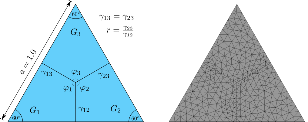
The first test corresponds to an academic triple junction test. Here the motion of MJs is dictated by the GB energies of the interfaces meeting at the central node. Fig. 3(left) illustrates this aspect, where the term $\displaystyle\gamma_{ij}$ denotes the GB energy between grains $\displaystyle G_{i}$ and $\displaystyle G_{j}$ and $\displaystyle\phi_{i}$ is the angle measured at the junction between the interfaces of grain $\displaystyle G_{i}$ and the other two grains. For this test, $\displaystyle\gamma_{13}=\gamma_{23}$, this will provoke a vertical movement of the junction for any value of $\displaystyle\gamma_{12}\neq\gamma_{23}$, until it arrives at its equilibrium position. As such, we will study the motion and the equilibrium of the junction in function of the ratio $\displaystyle r=\gamma_{23}/\gamma_{12}$. This test used dimensionless simulations, the value of the grain boundary energies $\displaystyle\gamma_{13}=\gamma_{23}=0.1$ and the mobility term $\displaystyle\mu=1$ were held constant, moreover, for practical reasons¹¹ 1 For $\displaystyle r<1$, the MJ moves downwards, which when using Neuman type boundary conditions, induce a global movement of the interfaces in the same direction, and eventually leads to the contact of the junction with the base of the triangle. This behaviour is not wanted in this context., Dirichlet boundary conditions with $\displaystyle\vec{v}_{i}=0\penalty\ \forall\penalty\ N_{i}\in\partial\Omega$ are imposed, hence impeding the movement of the nodes at the intersection of the GBs and the edges of the triangular domain. Finally, the mesh size parameter $\displaystyle h_{trm}=0.006$ and the time step $\displaystyle dt=5e-5$ will be used for all tests. These values were selected correspondingly to the limit of the stability region of the TRM model when using piece-wise polynomials (splines) as a means to obtain values of curvature, and normal [17]. The initial mesh is illustrated in Fig. 3(right).

While there is not an analytical formulation for the movement of the triple junction during its transient state in this context, triple junctions present stationary dihedral angles relying on the energies of the grain boundaries meeting at the junction [22]. In the absence of torque terms, i.e., when the energy of each interface is maintained constant, the dihedral angles $\displaystyle\phi_{1}$, $\displaystyle\phi_{2}$ and $\displaystyle\phi_{3}$ (see Fig. 3) verify the Young’s equilibrium, leading to the relation:

Similarly to [8], we tested ratios in the range of $\displaystyle r=[0.53,10]$, and the obtained equilibrium angles were compared to the analytical equilibrium state obtained thanks to Eq. 8. Fig. 4(left) illustrates the evolution of the $\displaystyle\varphi_{3}$ angle for different values of r obtained with the TRM model. These values are compared to the ones obtained in [8] (see Fig. 4(right)), where we have found that the TRM model evolves faster to its equilibrium state than the heterogeneous FE-LS method for values of $\displaystyle r>1.67$. Also, the TRM model can reproduce more accurately the analytical values of $\displaystyle\varphi_{3}$ for $\displaystyle r<1.0$. Fig. 5 also illustrates this aspect, where the final value of $\displaystyle\varphi_{3}$ is plotted against the grain boundary energy ratio $\displaystyle r$ and compared to the analytical equilibrium value via an L2-Error plot.

Figure 6 illustrates the final interface states for both approaches at the end of the simulation. In [8] it was found that, while the equilibrium angles of $\displaystyle\phi_{3}$ were accurately described for values of $\displaystyle r>2.5$ near the junction, the behaviour of the interfaces was strongly affected by the boundary conditions applied to the FE resolution, inducing non-minimal energy configurations. This behaviour was not found nor expected with the TRM model as boundary conditions only affect the velocity of nodes belonging to the boundary, and as a result, the TRM model reduces in all cases (until the equilibrium) the total energy of the system. This result can be found in Fig. 7 where the evolution of the normalised GB energy $\displaystyle\overline{E}_{\Gamma}$ (each curve was scaled to start from a value equals to 1), has been plotted as a function of time.

Similarly to the triple junction test, in this section we reproduce the same testing approach of [9] for heterogeneous FE-LS simulations of 2D-GG.

The first set of simulations measures the accuracy of the TRM model to reproduce results using different sets of mesh size and time step ($\displaystyle h_{trm},dt$). Results of these simulations are given in Appendix A.3. These simulations used a Read-Shockley (RS) type function [27] for the determination of the GB energy $\displaystyle\gamma$ as a function of the disorientation angle $\displaystyle\theta$:

where $\displaystyle\gamma_{max}$ is the maximal grain boundary energy equals to $\displaystyle 1.012\penalty\ Jm^{-2}$, $\displaystyle\theta_{max}$ corresponds to a threshold angle of $\displaystyle 30^{\circ}$ and the mobility term $\displaystyle\mu$ has been held constant and equal to 0.1 $\displaystyle mm^{4}J^{-1}s^{-1}$. These values are identical to the ones used in [9] for pure Nickel at 1400 $\displaystyle K$, where the authors have explained that contrary to the common usage of the RS function (using values for $\displaystyle\theta_{max}$ in the range of [10, 15] ^∘) a value of $\displaystyle\theta_{max}=30^{\circ}$ enables to numerically increase the system’s heterogeneity.

However, even with this choice, the heterogeneity level using a RS type function remains minimal. Indeed, only a narrow percent of the grain boundaries present a disorientation angle in the ”variational” zone of the RS function (see Fig. 15(bottom-right) for the values with a disorientation angle $\displaystyle\theta<30^{\circ}$.) while the majority of the interfaces present a disorientation angle $\displaystyle\theta\geq 30^{\circ}$, and thus they acquire a value of $\displaystyle\gamma=\gamma_{max}$. In [9], as a means to extend the representativity of the heterogeneous LS-FE formulation, multiple functions were used to compute the value of $\displaystyle\gamma$ as a function of $\displaystyle\theta$. This section will test the TRM model using two of the proposed functions. As such, the results presented here can be directly compared to those detailed in [9]. These functions correspond to the Read-Shockley+ and the Gaussian functions, which produce the most heterogeneous configurations. These functions are defined as follows:

RS+

where $\displaystyle\gamma_{max}^{\prime}=1.1\penalty\ Jm^{-2}$ and $\displaystyle\theta_{thresh}=55^{\circ}$

Gaussian

where $\displaystyle\gamma_{q}^{\prime}=1.54\penalty\ Jm^{-2}$, $\displaystyle\theta_{\mu}=40^{\circ}$ and $\displaystyle\theta_{\sigma}=10^{\circ}$

These formulations were used along with the RS function and a homogeneous formulation ($\displaystyle\gamma=1.012\penalty\ Jm^{-2}$) in the TRM model for the full-field modelling of annealing. These simulations were performed over four different initial Laguerre-Voronoi tessellations [28] based on an optimized sphere packing algorithm [29] and representative of the same statistical grain size distribution given in [9] with approximately 40000 grains each. One example of initial tessellation is given in Fig. 8. Hereafter, all results will contain data taken from the results of the four initial states and mean quantities will be averaged. Fig. 9 shows the evolution of this tessellation in time and for different $\displaystyle\gamma$ functions, here, the colours are representative of the GB energy of each interface. These figures illustrate how the RS formulation is too “homogeneous”, presenting just a few variations in the GB properties (even at the end of the simulation), while the RS+ and Gaussian are more heterogeneous. Additionally, in the RS+ and Gaussian cases, interfaces with a high GB energy seem to be eliminated during the early stages of the simulations, giving a higher predominance to low-energy GBs, which is not the case for the RS configuration. Another essential aspect observed in the final states of the RS+ and Gaussian cases is the appearance of stable high-order multiple junctions as predicted in section 2.2.

Figure 10 illustrates the normalised GB disorientation distributions of the heterogeneous configurations for every hour of annealing. Results show how the RS maintains its shape near the Mackenzie plot, hence not giving almost any preference to low energy GBs. Contrarily, the Gaussian and RS+ cases tend to avoid the disorientation angles with high energy. The plot shows maximum values at disorientation angles with low energy (e.g., for the RS+ configuration, finds one maximum at $\displaystyle\theta>\theta_{thresh}=55^{\circ}$). These results can also be observed in terms of the normalised grain boundary energy distributions given in Fig. 11. In only one hour of annealing, the Gaussian and RS+ configurations tend to dissipate high energy GBs, giving a much higher predominance to low energy GBs and promoting their permanency (or their appearance) as time advances. In contrast, for the RS configuration, the changes in the distribution of energy remain negligible. The Gaussian configuration is a perfect example of how the TRM algorithm respond to grain boundary energy minimisation when opposed to a highly heterogeneous configuration.

Low energy GBs predominance may produce a deceleration of the evolution of the grain size in the domain. Fig. 12 illustrates the grain size distribution of the different test cases showing how the RS configuration produces a grain size distribution with larger sizes while the RS+ and Gaussian configurations promote smaller grains.

Fig. 13 gives the evolution of the mean grain size, the total number of grains, the total GB energy, and the total grain boundary length. The minimisation of the GB energy is much higher for the most heterogeneous cases (RS+ and Gaussian), even though their number of grains and mean size appears to have a ”slower” evolution than the RS and homogeneous cases. Also, the responses of the homogeneous and the RS cases are very similar.

Fig. 14(b) gives the total GB length plotted against the number of grains of the simulation showing how the Gaussian and RS+ cases have a higher value than the RS and the homogeneous cases. This result can not be anticipated as one could have guessed the contrary, by seeing the evolution curves of the total GB energy given in Fig. 13(bottom-left) as a function of time and as illustrated in Fig. 14(a) as a function of the number of grains. This result is a product of the preference of the higher heterogeneous cases for grain boundaries of low energy, but also by the more frequent apparition of high-order multiple junctions that decelerate the reduction of the total GB length.

Table 13 gives the CPU-time of each simulation, showing how the computational cost of the TRM model in this context may be more related to the length of boundaries than to the number of grains (see Fig. 14b)). Additionally, the differences between the computational cost of the homogeneous and the heterogeneous cases are very high. This can be explained by the fact that for the homogeneous case, it is not necessary to compute the misorientation at GBs nor the lowest energy configuration in the event of a separation of MJs. These operations are very demanding as both rely on an iterative computation of the lowest rotation angle between two orientations in a set of 24 possible rotations, where all of them have to be tested. Table 13 also shows that, the higher the heterogeneity of the case, the higher is its computational cost. This behaviour can be anticipated by seeing the evolution of the number of grains and the total length of boundaries (Fig. 14), as the more homogeneous cases reduce these quantities much faster.

The results presented here are very similar to the ones obtained in [9] in the context of the heterogeneous FE-LS formulation. This suggests that both methodologies are valid to predict microstructural states in a full-field context, as even though the mechanisms behind their evolution are the same, they have been modelled using a completely different numerical scheme and still produce a very similar outcome. It mush be highlighted that simulations in [9] where performed with initial states with around 5000 grains while here we performed simulations 8 times larger (for simulations using the same initial grains as in [9] see [30]). Moreover, the computational power needed to produce these results using the heterogeneous FE-LS may be much higher than the one needed by the TRM. The TRM model performed all sequential simulations in less than eight hours for the heterogeneous configurations and in less than one hour for the homogeneous ones, using an AMD Ryzen 7 3600x processor.

References

- [1] J. Humphreys, G. S. Rohrer, A. Rollett, Recrystallization and Related Annealing Phenomena (Third Edition), Elsevier, 2017. doi:10.1016/B978-0-08-098235-9.00004-5.
- [2] T. Watanabe, Grain boundary engineering: historical perspective and future prospects, Journal of materials science 46 (12) (2011) 4095–4115.
- [3] J. Fausty, Towards the full field modeling and simulation of annealing twins using a Finite Element Level Set method., Ph.D. thesis, PSL, Mines-ParisTech (2020).
- [4] J. Fausty, B. Murgas, S. Florez, N. Bozzolo, M. Bernacki, A new level set-finite element formulation for anisotropic grain boundary migration (jun 2020). arXiv:2006.15531.
- [5] B. Murgas, S. Florez, N. Bozzolo, J. Fausty, M. Bernacki, Comparative study and limits of different level-set formulations for the modeling of anisotropic grain growth (2021). arXiv:2106.03565.
- [6] G. DeWit, J. S. Koehler, Interaction of dislocations with an applied stress in anisotropic crystals, Phys. Rev. 116 (1959) 1113–1120. doi:10.1103/PhysRev.116.1113.
- [7] G. S. Grest, D. J. Srolovitz, M. P. Anderson, Computer simulation of grain growth-IV. Anisotropic grain boundary energies, Acta Metallurgica 33 (3) (1985) 509–520. doi:10.1016/0001-6160(85)90093-8.
- [8] J. Fausty, N. Bozzolo, D. Pino Muñoz, M. Bernacki, A novel level-set finite element formulation for grain growth with heterogeneous grain boundary energies, Materials & Design 160 (2018) 578–590.
- [9] J. Fausty, N. Bozzolo, M. Bernacki, A 2D level set finite element grain coarsening study with heterogeneous grain boundary energies, Applied Mathematical Modelling 78 (2020) 505–518. doi:10.1016/j.apm.2019.10.008.
- [10] E. Miyoshi, T. Takaki, Multi-phase-field study of the effects of anisotropic grain-boundary properties on polycrystalline grain growth, Journal of Crystal Growth 474 (November 2016) (2017) 160–165. doi:10.1016/j.jcrysgro.2016.11.097.
- [11] H. Hallberg, V. V. Bulatov, Modeling of grain growth under fully anisotropic grain boundary energy Modeling of grain growth under fully anisotropic grain boundary energy, Modelling and Simulation in Materials Science and Engineering 27 (045002) (2019).
- [12] L. A. Barrales Mora, 2D vertex modeling for the simulation of grain growth and related phenomena, Mathematics and Computers in Simulation 80 (7) (2010) 1411–1427. doi:10.1016/j.matcom.2009.08.005.
- [13] M. Elsey, S. Esedog¯lu, P. Smereka, Simulations of anisotropic grain growth: Efficient algorithms and misorientation distributions, Acta Materialia 61 (6) (2013) 2033–2043. doi:10.1016/J.ACTAMAT.2012.12.023.
- [14] C. Mießen, N. Velinov, G. Gottstein, L. A. Barrales-Mora, A highly efficient 3D level-set grain growth algorithm tailored for ccNUMA architecture, Modelling and Simulation in Materials Science and Engineering 25 (8) (2017). arXiv:1701.06658, doi:10.1088/1361-651X/aa8676.
- [15] K. Kawasaki, T. Nagai, K. Nakashima, Vertex models for two-dimensional grain growth, Philosophical Magazine B 60 (3) (1989) 399–421. doi:10.1080/13642818908205916.
- [16] K. Chang, L. Q. Chen, C. E. Krill, N. Moelans, Effect of strong nonuniformity in grain boundary energy on 3-D grain growth behavior: A phase-field simulation study, Computational Materials Science 127 (2017) 67–77. doi:10.1016/j.commatsci.2016.10.027.
- [17] S. Florez, K. Alvarado, D. P. Muñoz, M. Bernacki, A novel highly efficient Lagrangian model for massively multidomain simulation applied to microstructural evolutions, Computer Methods in Applied Mechanics and Engineering 367 (2020) 113107. doi:10.1016/j.cma.2020.113107.
- [18] S. Florez, J. Fausty, K. Alvarado, B. Murgas, M. Bernacki, Parallelization of an efficient 2d-lagrangian model for massive multi-domain simulations, To appear in Modelling and Simulation in Materials Science and Engineering (preprint at arXiv:2009.04424, 2020). arXiv:2009.04424.
- [19] S. Florez, K. Alvarado, M. Bernacki, A new front-tracking lagrangian model for the modeling of dynamic and post-dynamic recrystallization, Modelling and Simulation in Materials Science and Engineering 29 (3) (2021) 035004. doi:10.1088/1361-651x/abd837.
- [20] S. Florez, K. Alvarado, M. Bernacki, Statistical behaviour of interfaces subjected to curvature flow and torque effects applied to microstructural evolutions (2021). arXiv:2106.05605.
- [21] J. K. Mackenzie, Second paper on statistics associated with the random disorientation of cubes, Biometrika 45 (1-2) (1958) 229–240. doi:10.1093/biomet/45.1-2.229.
- [22] C. Herring, Surface tension as a motivation for sintering, in: Fundamental Contributions to the Continuum Theory of Evolving Phase Interfaces in Solids, Springer, 1999, pp. 33–69.
- [23] R. Stanley, Enumerative combinatorics, Cambridge University Press, Cambridge, 1999.
- [24] B. Merriman, J. K. Bence, S. J. Osher, Motion of Multiple Junctions: A Level Set Approach, Journal of Computational Physics 112 (2) (1994) 334–363. doi:10.1006/jcph.1994.1105.
- [25] M. Bernacki, Y. Chastel, T. Coupez, R. E. Logé, Level set framework for the numerical modelling of primary recrystallization in polycrystalline materials, Scripta Materialia 58 (12) (2008) 1129–1132. doi:10.1016/j.scriptamat.2008.02.016.
- [26] B. Scholtes, M. Shakoor, A. Settefrati, P.-O. Bouchard, N. Bozzolo, M. Bernacki, New finite element developments for the full field modeling of microstructural evolutions using the level-set method, Computational Materials Science 109 (2015) 388–398. doi:10.1016/j.commatsci.2015.07.042.
- [27] W. T. Read, W. Shockley, Dislocation Models of Crystal Grain Boundaries, Physical Review 78 (3) (1950) 275–289. doi:10.1103/PhysRev.78.275.
- [28] K. Hitti, P. Laure, T. Coupez, L. Silva, M. Bernacki, Precise generation of complex statistical Representative Volume Elements (RVEs) in a finite element context, Computational Materials Science 61 (2012) 224–238. doi:10.1016/j.commatsci.2012.04.011.
- [29] K. Hitti, M. Bernacki, Optimized dropping and rolling (odr) method for packing of poly-disperse spheres, Applied Mathematical Modelling 37 (8) (2013) 5715–5722.
- [30] S. Florez, Towards highly efficient massive-multidomain simulations in the context of microstructural evolutions., Ph.D. thesis, PSL, Mines-ParisTech (2020).