Scale-Free Adversarial Multi Armed Bandits

The Adversarial Multi Armed Bandit(MAB) problem proceeds as a sequential game of $T$ rounds between a player and an adversary. In each round $t=1,\dots,T$, the player selects a distribution $p_{t}$ over the $n$-arms and the adversary selects a loss vector $l_{t}$ belonging to some set $\mathcal{L}\subseteq\mathbb{R}^{n}$. An action $i_{t}$ is sampled from $p_{t}$ and the player observes the loss $l_{t}(i_{t})$. The (expected) regret of the player is:

We assume that the adversary is oblivious, i.e., the loss vectors $l_{1},\dots,l_{T}$ are chosen before the game begins. So, the above expectation is with respect to the randomness in the player’s strategy. The goal of the player is to sequentially select the distributions $p_{1},\dots,p_{T}$ such that $R_{T}$ is minimized. The adversarial MAB problem has been studied extensively; we refer the reader to the texts of Bubeck and Cesa-Bianchi 2012; Lattimore and Szepesvári 2020; Slivkins 2019 for further details. Assuming that $\mathcal{L}$ is bounded, and the $\|\cdot\|_{\infty}$-Lipschitz constant $G$ is known to the player in advance (i.e. $\sup_{l\in\mathcal{L}}\|l\|_{\infty}=G<\infty$), the minimax rate of regret is known to be $\Theta(G\sqrt{nT})$. The Exp3 algorithm (Auer et al. 2002) has a $\mathcal{O}(G\sqrt{nT\log(n)})$ regret bound whereas the Poly-INF algorithm (Audibert and Bubeck 2009) removes the $\sqrt{\log(n)}$ factor, achieving the optimal $\mathcal{O}(G\sqrt{nT})$ regret bound. Exp3 and Poly-INF use $G$ in tuning the learning rate, which helps them achieve a linear dependence on $G$.

In this paper, we address the case when the player has no knowledge of $\mathcal{L}$. We consider Scale-Free bounds for MABs, which aim to bound the regret in terms of $n$ and norms of the loss vectors $l_{1},\dots,l_{T}$ for any sequence of loss vectors chosen arbitrarily by adversary. Scale-free bounds have been studied in the full-information setting (where the player sees the complete vector $l_{t}$ in each round). For the Experts problem, which is the full-information counterpart of adversarial MAB, the AdaHedge algorithm (de Rooij et al. 2014) has a scale-free regret bound of $\mathcal{O}(\sqrt{\log(n)(\sum_{t=1}^{T}\|l_{t}\|_{\infty}^{2})})$. For the same problem, the Hedge algorithm (Freund and Schapire 1997) has a regret bound of $\mathcal{O}(G\sqrt{T\log(n)})$ with knowledge of $G$. The scale-free bound is more general as it holds for any $l_{1},\dots,l_{T}\in\mathbb{R}^{n}$, whereas the bound achieved by the Hedge algorithm only holds provided that $\sup_{t}\|l_{t}\|_{\infty}<G$ where $G$ needs to be known in advance.

Consider for a moment, full-information strategies on $\Delta_{n}$. In the full information setting, in each round $t$, the player picks a point $p_{t}\in\Delta_{n}$. Simultaneously, the adversary picks a loss vector $l_{t}\in\mathbb{R}^{n}$. The player incurs a loss of $l_{t}^{\top}p_{t}$ and (unlike the bandit setting) sees the entire vector $l_{t}$. A full-information strategy $\mathcal{F}$ takes as input a sequence of loss vectors $l_{1},\dots,l_{t}$ and outputs the next iterate $p_{t+1}\in\Delta_{n}$. A MAB strategy $\mathcal{B}$ can be constructed from a full-information strategy $\mathcal{F}$ along with two other components as follows:

1. 1.

   A sampling scheme $\mathcal{S}$, which constructs a sampling distribution $p^{\prime}_{t}$ from the current iterate $p_{t}$. An arm $i_{t}$ is then sampled from $p^{\prime}_{t}$ and the loss $l_{t}(i_{t})$ is revealed to the player.

2. 2.

   An estimation scheme $\mathcal{E}$, that constructs an estimate $\tilde{l}_{t}$ of the loss vector $l_{t}$ using $l_{t}(i_{t})$ and $p_{t}$.

3. 3.

   A full-information strategy $\mathcal{F}$, which computes the next iterate $p_{t+1}$ using all the estimates $\tilde{l}_{1},\dots,\tilde{l}_{t}$.

In fact, most existing MAB strategies in the literature can be described in the above framework with different choices of ${\cal S},{\cal E},{\cal F}$.

A delicate balance needs to be struck between $\mathcal{S},\mathcal{E}$ and $\mathcal{F}$ in order to achieve a good regret bound for $\mathcal{B}$. Suppose the best arm in hindsight is $i_{\star}=\arg\min_{i\in[n]}\sum_{t=1}^{T}l_{t}(i)$ The expected regret of MAB strategy $\mathcal{B}$ can be decomposed as follows:

Term (1) is due to the sampling scheme $\mathcal{S}$, term (2) is the effect of the estimation scheme $\mathcal{E}$ and term (3) is the expected regret of the full-information strategy $\mathcal{F}$ on the loss sequence $\tilde{l}_{1},\dots,\tilde{l}_{T}$ compared to playing the fixed strategy $\textbf{1}^{i^{\star}}$.

The regret of $\mathcal{F}$ has an component called the stability term $\Psi_{p}:\mathbb{R}^{n}\to\mathbb{R}$. In the bandit case, $\mathcal{F}$ receives the IW estimates $\tilde{l}_{t}$. So, it is important that the stability term be bounded with IW estimates. Without going into any technical details, we note that it is desirable to have a stability term bounded by $\Psi_{p}(l)\leq p^{\top}l^{2}$ as its expectation with IW estimates can be bounded.

Previous techniques to bound the stability term by $p^{\top}l^{2}$ relied on the assumptions on $l$, such as either $l\geq\textbf{0}$ or $l\geq-\textbf{1}$ (See (Lattimore and Szepesvári 2019, Page 5)). For arbitrary $l\in\mathbb{R}^{n}$, we show that it is possible to bound the stability term by $p^{\top}l^{2}$ using the log-barrier regularizer. The procedure we develop to obtain this bound is the main technical contribution of our paper.

The complete algorithm for the scale-free MAB problem is described below. We give two choices for the exploration parameter $\gamma_{t}$. A simple non-adaptive scheme that is similar to the one in Hadiji and Stoltz 2020, where $\gamma_{t}\propto\frac{1}{\sqrt{t}}$ and an adaptive scheme that picks $\gamma_{t}$ in a fashion that resembles the adaptive learning rate scheme $\eta_{t}$.

Scale-Free Multi Armed Bandit\DontPrintSemicolonStarting Parameters: $\eta_{0}=n,\gamma_{0}=1/2$  Regularizer $\displaystyle F(q)=\sum_{i=1}^{n}(f(q(i))-f(1/n))$, where $f(x)=-\log(x)$  First iterate $p_{1}=(1/n,\dots,1/n)$  \For$t=1$ to $T$ Sampling Scheme: $\displaystyle p^{\prime}_{t}=(1-\gamma_{t-1})p_{t}+\frac{\gamma_{t-1}}{n}$  Sample Arm $i_{t}\sim p^{\prime}_{t}$ and see loss $l_{t}(i_{t})$.  Estimation Scheme: $\displaystyle\tilde{l}_{t}=\frac{l_{t}(i_{t})}{p^{\prime}_{t}(i_{t})}\textbf{1}^{i_{t}}$  Compute $\gamma_{t}$ for next step:
(Option 1) Non-adaptive $\gamma_{t}=\min(1/2,\sqrt{n/t})$
(Option 2) Adaptive $\displaystyle\gamma_{t}=\frac{n}{2n+\sum_{s=1}^{t}\Gamma_{s}(\gamma_{s-1})}$ where $\displaystyle\Gamma_{t}(\gamma)=\frac{\gamma|l_{t}(i_{t})|}{(1-\gamma)p_{t}(i_{t})+\gamma/n}$  Compute $\displaystyle\eta_{t}=\frac{n}{1+\sum_{s=1}^{t}M_{s}(\eta_{s-1})}$ where $\displaystyle M_{t}(\eta)=\sup_{q\in\Delta_{n}}\left[\tilde{l}_{t}^{\top}(p_{t}-q)-\frac{1}{\eta}\text{Breg}_{F}(q\|p_{t})\right]$  Find next iterate using FTRL: $\displaystyle p_{t+1}=\arg\min_{q\in\Delta_{n}}\left[F(q)+\eta_{t}\sum_{s=1}^{t}q^{\top}\tilde{l}_{s}\right]$ Our main result is the following regret bound for Algorithm 2.

We begin by recalling a few definitions.

For instance, the function $x\log(x)-x$, $-\sqrt{x}$, $-\log(x)$ are all Legendre on $(0,\infty)$

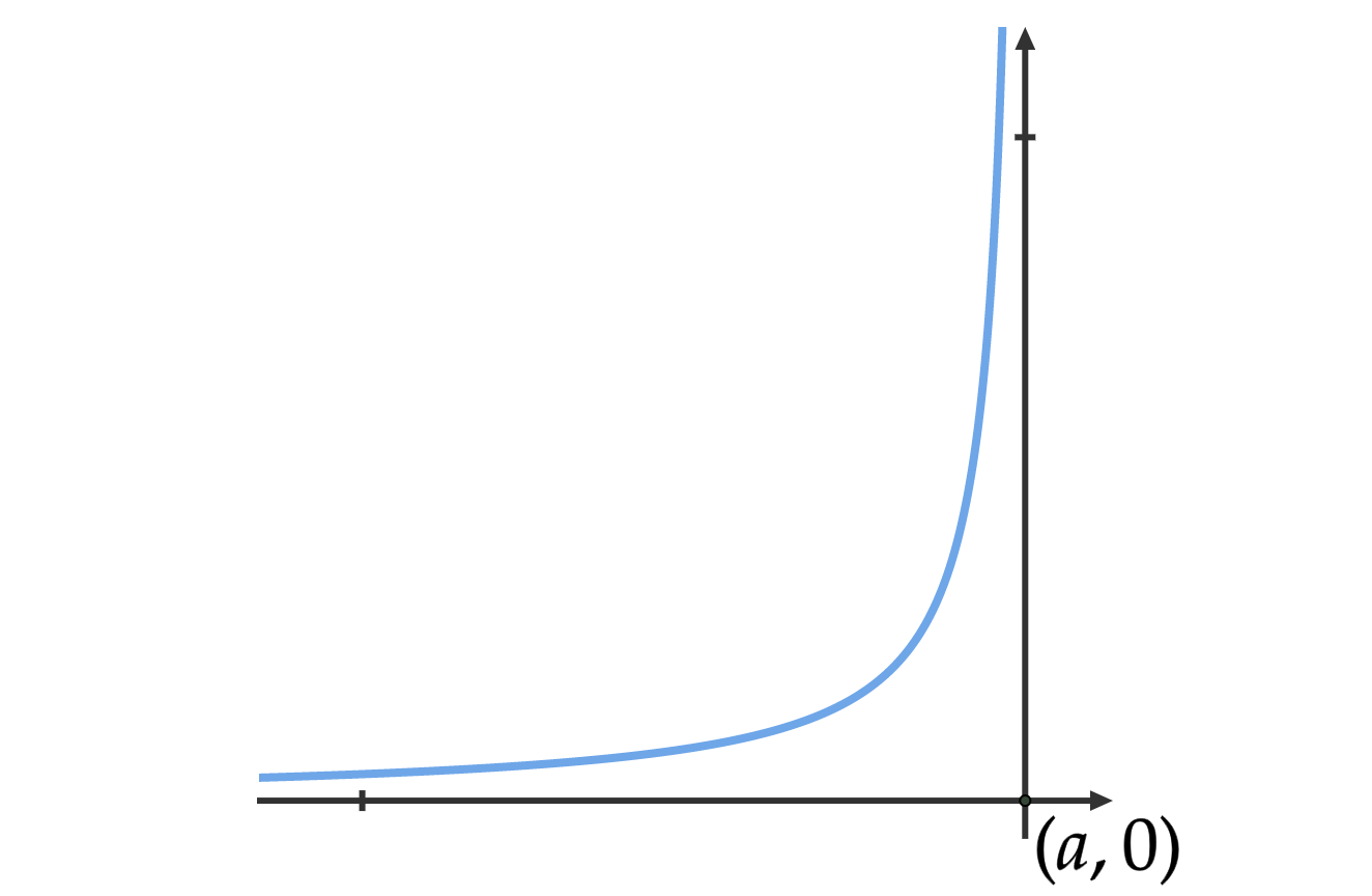
For instance, $\exp(x)$ is a potential with $a=\infty$ and $-1/x$ is a potential with $a=0$. A potential function typically looks like Figure 1. Potentials were introduced in Audibert and Bubeck 2009; Audibert et al. 2011; Audibert et al. 2014 for analyzing the Implicitly Normalized Forecaster(INF) algorithm, of which Poly-INF is a specific case.

Associated with a potential $\psi$, we define a function $f_{\psi}$ as the indefinite integral $f_{\psi}(z)=\int\psi^{-1}(z)dz+C$. Since the domain of $\psi^{-1}$ is $(0,\infty)$, the domain of $f_{\psi}$ is also $(0,\infty)$. For instance, if $\psi(x)=-1/x$ on the domain $(-\infty,0)$, the associated function is $f_{\psi}(x)=-\log(x)+C$.

Observe that $f_{\psi}^{\prime}(z)=\psi^{-1}(z)$ and $f_{\psi}^{\prime\prime}(z)=\left[\psi^{\prime}(\psi^{-1}(z))\right]^{-1}$. Since $\psi$ is strictly convex and increasing, $\psi^{\prime}>0$ and thus $f^{\prime\prime}_{\psi}>0$, making $f_{\psi}$ strictly convex. Moreover, $\lim_{z\to 0}\mid f_{\psi}^{\prime}(z)\mid=\lim_{z\to 0}\mid\psi^{-1}(z)\mid=+\infty$. Thus $f_{\psi}$ is a Legendre function on $(0,\infty)$. Define the function $F_{\psi}:\mathbb{R}^{n}\to\mathbb{R}$ as $F_{\psi}(x)=\sum_{i=1}^{n}[f_{\psi}(x(i))-f_{\psi}(1/n)]$. This function is Legendre on $(0,\infty)^{n}$.

Given a potential $\psi:(-\infty,a)\to(0,+\infty)$ and its associated function $f_{\psi}$, the Legendre-Fenchel dual of $f_{\psi}$ is $f_{\psi}^{\star}:(-\infty,a)\to\mathbb{R}$ defined as $f_{\psi}^{\star}(u)=\sup_{z>0}(zu-f_{\psi}(z))$. The supremum is achieved at $z={f^{\prime}_{\psi}}^{-1}(u)=\psi(u)$. So we have that $f_{\psi}^{\star}(u)=u\psi(u)-f_{\psi}(\psi(u))$. This implies ${f_{\psi}^{\star}}^{\prime}(u)=\psi(u)$ and ${f_{\psi}^{\star}}^{\prime\prime}(u)=\psi^{\prime}(u)$. Further, using integration by parts on $\int\psi(u)du$ and substituting $\psi(u)=s$:

Thus $f^{\star}_{\psi}(u)=\int\psi(u)du-C$. Here $C$ is the same constant of integration picked when defining $f_{\psi}(z)=\int\psi^{-1}(z)dz+C$. We have the following property (proof in Appendix A):

Let $\psi$ be a potential and $x,y\in\mathbb{R}_{+}$. We show a general way of obtaining lower-bounds using potential functions, that are of the form:

Where $w$ is some positive function.

In the context of online learning, local-norm lower-bounds have been studied before, see for example Orabona 2019. However, these relied upon Taylor’s theorem to show that $\text{Breg}_{f_{\psi}}(y\|x)=\frac{1}{2}(x-y)^{2}f^{\prime\prime}_{\psi}(z)$ for some $z\in[x,y]$. Then, they used further conditions on $x,y$ to argue that $cf^{\prime\prime}_{\psi}(x)\leq f^{\prime\prime}_{\psi}(z)$ for some positive constant $c$ and thus arrive at $\text{Breg}_{f_{\psi}}(y\|x)\geq\frac{c}{2}(x-y)^{2}f^{\prime\prime}_{\psi}(x)$. We generalize this argument in Lemma 6, through which we are able to generate a more rich class of lower-bounds. We illustrate with an example below:

The result of Corollary 7 is illustrated in Figure 4. The shaded region is $\{(x,y):x\geq 0,y\geq 0,\frac{y}{x}-1-\ln\left(\frac{y}{x}\right)\geq\frac{1}{2}\frac{(x-y)^{2}}{x}\}$. Clearly the region $\{(x,y):0\leq x\leq 1,0\leq y\leq 1\}$ is within the shaded region.

The iterates of FTRL with the regularizer $F_{\psi}(x)=\sum_{i=1}^{n}[f_{\psi}(x(i))-f_{\psi}(1/n)]$ for some potential function $\psi$ and positive learning rates $\{\eta_{t}\}_{t=0}^{T}$, are of the form:

Since $F_{\psi}$ is Legendre, the point $p_{t+1}$ always exists strictly inside $\Delta_{n}$. Orabona 2019 and Joulani et al. 2017; Joulani et al. 2020 provide general purpose regret analysis of FTRL. For the sake of completeness, we show a simple way of analyzing FTRL when the action set is $\Delta_{n}$ and the regularizer chosen is of the form $F_{\psi}(x)=\sum_{i=1}^{n}[f_{\psi}(x(i))-f_{\psi}(1/n)]$ in Appendix C.

The AdaFTRL strategy picks a specific sequence of learning rate $\eta_{t}$ based on the history $H_{t}$. This strategy was analyzed in Orabona and Pál 2018 and a simpler analysis was given by Koolen 2016. Our analysis is adapted from Hadiji and Stoltz 2020. We consider the adaptive learning rate:

Where $M_{t}(\eta)=\sup_{q\in\Delta_{n}}\left[l_{t}^{\top}(p_{t}-q)-\frac{1}{\eta}\text{Breg}_{F_{\psi}}(q\|p_{t})\right]$, is the Mixability Gap and $\alpha,\beta>0$. Since $q=p_{t}$ is a feasible solution for this optimization problem, we have $M_{t}(\eta)\geq 0$. Let $p_{t}^{\star}$ be the optimal value of $q$ in the optimization. We have the upper bound

Since $M_{t}(\eta)$ are non-negative and bounded, the sequence $\eta_{t}$ is non-increasing.

See 1