Stability of topological purity under random local unitaries
Abstract
In this work, we provide an analytical proof of the robustness of topological entanglement under a model of random local perturbations. We define a notion of average topological subsystem purity and show that, in the context of quantum double models, this quantity does detect topological order and is robust under the action of a random quantum circuit of shallow depth.
Introduction
Topological order[1] is a novel kind of quantum order that goes beyond the paradigm of symmetry breaking. Its role is prominent in condensed matter theory as well as in quantum computation. In particular, topological order can be employed to construct various models for robust quantum memory and logic gates[2, 3]. Topologically ordered states show patterns of non local quantum entanglement that cannot be detected by a local order parameter. However, the long-range quantum entanglement leaves its mark in the reduced density matrix, and a series of papers have shown that topological order can be detected by the topological entropy[4, 5, 6]: a topological correction to the area law for the entanglement entropy. In particular, topological entanglement entropy has been employed to characterize the ground state of different models[7, 8, 9, 10, 11, 12, 13, 14, 15, 16, 17] Recent works have shown that this type of long-range quantum entanglement together with the topological entropy is robust against local perturbation of the Hamiltonian[18, 19, 20] and small deformation of partition geometry. Attempts at showing the robustness of the topological order under local perturbations[21, 22] are either a proof of the stability of the phase or are often limited to specific examples and are mostly of numerical nature or resort to quantum field theory arguments[5], while an analytical proof for the robustness of topological entropy in lattice models is still lacking[23, 24, 25]. In this work, we provide an analytic proof of the robustness of topological order under a noise model consisting of random local unitaries. To this end, we construct a notion of average topological subsystem purity that captures the same long-range pattern of entanglement of topological entanglement entropy, and we show that such topological purity is constant if the circuit is shallow compared to the relevant size of the subsystem (which, can be made scale with the size of the whole system ).
We work in the framework of quantum double models on the cyclic group introduced by Kitaev in [2], and define the topological purity (TP), which is related to the topological Rényi entropy defined in [26]. There are many reasons to use purity instead of entanglement entropy in order to argue about questions about quantum many-body systems. Unlike the Von Neumann entanglement entropy (whose measurement requires a complete state tomography of the system[27]), the Rényi entropy is directly related to the purity which is an observable and can be measured directly[28, 29, 30, 31, 32] as it is the expectation value of the swap operator over two copies of the system. This quantity contains substantial information about the universal properties of quantum many-body systems[33] and it is able to reveal the topological pattern of entanglement[26, 34]. This property makes purity also amenable analytical treatment[35, 36, 37, 38, 39, 40].
To prove the robustness of topological order by the topological purity we introduce, as a noise model, a set of quantum maps whose action on a state is based on local random (shallow) quantum circuits. We find that the topological purity distinguishes two phases of states, attaining two different constant values. When the circuit depth is comparable with the subsystem size, the long-range pattern of entanglement that is responsible for topological order can be changed and the topological purity can change value. The phase is then indeed the orbit of the so defined set of quantum maps through a reference state. The proof is obtained thanks to two key non trivial facts: (i) the subsystem purity of the ground state of quantum double models only depends on the geometry of its boundary, while the topological purity only depends on its topology, and (ii) the action of the specific noise model we work with can be regarded as the evolution of that boundary. Since the maps are shallow, their action will result in a local deformation of the subsystem boundary that does not alter their topology, and, by (i), this will result in an exactly constant topological purity. Similarly, we show that the topological purity of a topologically trivial state is zero and that it cannot be changed by our noise model.
The paper is organized as follows: in Sec.1 we review quantum double models; in Sec.2 we introduce the topological purity and discuss how it is connected with other measures of topological entropy; in Sec.3.1 we introduce the noise model and finally in Secs.3.2 and 3.3, will be devoted to the rigorous proof of our result and will be rather technical.
1 Quantum Double models on
Quantum double models are exactly solvable models defined on a lattice[2]. Consider the cyclic finite group with and local Hilbert spaces and the total Hilbert space given by the tensor product of local Hilbert spaces, namely placed at the bonds of a square lattice , see Fig.1. The dimension of the total Hilbert space is thus . Let be an orthonormal basis in .

For each local Hilbert space we introduce the operators defined through their action on the ket :
| (1) |
where times and the addition is modulo . Consider the enlarged operators and acting non trivially only on the site . Define the following operators acting non trivially on the subset , sketched in Fig.1:
| (2) |
note that (plaquette operator) and (star operator) are projectors. At this point, the Hamiltonian of the quantum double model reads:
| (3) |
and the ground state manifold is given by:
| (4) |
To represent the ground state in terms of the spin degrees of freedom, let us introduce the group generated by all the operators, defined as . The state defined as
| (5) |
is a state in , as it can be readily checked. Other basis states in can be constructed by the use of non contractible loop operators[2]. The topological order in this model can be detected by the entanglement entropy in the ground state manifold. Consider a bipartition in the Hilbert space, namely and compute the reduced density matrix [26]:
| (6) |
where and we introduced and that are normal groups in , and the quotient groups and . Following [26] we can prove that and thus the purity is given by , i.e one can argue that the purity is counting the number of independent operators acting non trivially on both regions and . Following [4], given a region , the number of operators acting on both subsystems and is where is the cardinality of the boundary of , i.e the number of sites in having at least one nearest neighbor inside , and , for , is the number of sites in having nearest neighbors inside . Thus is a geometrical correction which depends on the shape of the region . For example, if is a convex loop (a rectangle) . So far we accounted for the number of star operators acting on both subsystems, but not all of them are independent from each other because of the constraints on the ground state manifold in (4), in particular the condition . Following [4, 6] and defining as the number of boundaries of , we have that the number of independent star operators is , i.e for each boundary of we have that the number of independent star operators acting on both subsystems decreases of a factor scaling as . We thus can finally write the following:
| (7) |
where is the sum of a geometrical term which depends on the shape of the boundary and a topological correction , due to the actual number of independent star operators, only related to the topology of . This topological correction is called topological entropy[4, 6, 5]. Eq.(7) is of fundamental importance for the reminder of the paper: it is telling us that the purity of the reduced density matrix in the ground state manifold of the topologically ordered quantum double model depends on the boundary only.
2 The topological purity
In this section, we show how the topological pattern of entanglement involved in topologically ordered states[1] can be also found in a new quantity: the topological purity (TP). To understand heuristically how this quantity works, let us first introduce the topological entropy: consider the state living in the Hilbert space and the regions and drawn in Fig.2 . The topological entropy is defined as
| (8) |
where labels the Von Neumann entropy of where is the complement of with respect to . As it was shown in[26], also all the Renyi topological entropies give exactly the same results for the quantum double models. The definition of the topological entropy is equal to minus the quantum conditional information [41], which is a entropic quantity describing tripartite correlations of quantum states.

In the same fashion of Eq.(8), the topological purity is defined as:
| (9) |
i.e. the ratio of purities of the reduced density matrix of a quantum state in the four subsystems , , and . The purity of in the subsystem is defined as , where is the complement of . By definition,
| (10) |
is just the topological 2-Rényi entropy. Consider the domain in Fig.2 , then for each and since , the topological purity is just given by the sum of the geometrical corrections
| (11) |
where is the topological entropy[6]. Note that, according to the discussion in the previous section, all the geometrical corrections related to the shape of the boundary are canceled by the choice of the partitions , namely , and the only surviving term is the topological correction that does not depend on the shape of the boundary: it is a purely topological correction . This correction is the mark of the topological phase. It is worth noting that the topological correction would not be detected from the topological purity if was a simply connected region as the one sketched in Fig.2, see also [6]. That is because, as shown in the previous section, the number of boundaries gives the number of topological corrections to the purity of the related subsystem . Specifically, consider Fig.2 first: we have , and thus according to Eq.(11) we have , while for Fig.2 : and , thus .
In [5], it was argued, through TQFT arguments, that a local deformation of the boundary will not affect the topological entropy. For the lattice model, we can prove the following lemma that affirms the same property:
Lemma 1.
The TP for the state is stable under local boundary deformations.
Proof. Consider a subset and consider the boundary transformation . Let us suppose, without loss of generality, that , cfr. Fig.2 . Thus, according to Eq.(7), we have:
| (12) | |||||
| (13) |
while and are unmodified. Then note that and that because .
The request of the boundary modification being local is extremely important. Indeed, it is always true that, as sets, . However, only if the boundary modifications are local then the number of disconnected boundaries is unchanged.
The above lemma is necessary for the TP to be a good detector of the TO. In particular, if , then is a trivial topological state, while if , is expected to be in a non trivial topological phase.
3 Stability of topological purity
In this section, we establish a noise model based on quenched disorder, and show how the topological order behaves under the noise model. We consider a random local unitary noise on the spins in the lattice. Under this noise model, one can compute the average purity in a subsystem due to this noise. This is the purity one would measure in an experiment if the measurement time-scales are much longer than the random fluctuations in the unitary noise. Then one can define a topological purity associated with these average purities. If the noise is zero, the average is just the purity of the initial state, and the two topological purities coincide.
We want to show that, if the random unitaries build up a shallow quantum circuit, then the topological purity is constant. The proof is quite technical, so let us first give an intuitive explanation. We first show that, the purity in the subsystem averaged over all the transformations of the state under the noise model is equal to the purity in the initial state for a subsystem with a different boundary, depending only on which spins were affected by the random quantum noise. It is a very non trivial fact that under such kind of noise, the average purity results in just a boundary transformation for the purity in the initial state. Then it follows that, if the noise is shallow, only shallow deformations of the boundary are possible, and by Lemma 1 the topological purity is preserved.
3.1 Topological purity and phases
Let us now dive into the technical details of the noise model and the robustness of topological purity. Let be the dimensional Hilbert space of qudits in a set . Here, the Hilbert space of the th qudit is denoted by . Let be a subset of these qudits and the corresponding Hilbert space. Let be the order two permutation (swap) operator on and let be its trivial completion on the full .
The purity of the state in the bipartition is given by
| (14) |
where . The above chain of relations is telling us that the purity is from both the analytical point of view and the experimental point of view a quantity defined on two copies of the Hilbert space . In practice, in order to experimentally measure the purity of a quantum state in a given bipartition , one needs three steps: to prepare two identical copies of , to build the observable swap operator on the subspace and finally, to take the quantum expectation value of in , namely . Similarly, in order to experimentally measure the topological purity, defined in Eq.(9), one needs to repeat the steps , and for the four observables and then combine them in the following way:
| (15) |
Since the purity is defined on , we define a noise model on states living on two copies of the Hilbert space in the following way: let be a set of qudits with Hilbert space and . Let be a local unitary operator operating on the region , i.e. operating on all the qubits contained in . Let be two copies of , then after operating on with the unitary , we have and the purity becomes
| (16) |
We now choose to be a random unitary operator and define the following quantum map acting on :
| (17) |
where is the Haar measure over the unitary group . Therefore, fixed , the map randomizes over the action of the full unitary group on . Thus, after the noise on , the purity becomes:
| (18) |
note that the above operation is no more acting independently on the single copies of , but it is entangling them in . So far this is a single noise model. In order to generalize it to more than one single domain, consider an ordered string of subsets and random unitary operators operating on the corresponding subset and acting on in an ordered way, namely . We define the quantum map randomizing over the action of these gates as:
| (19) |
where
| (20) |
For each string of domains , the action of on a state of describes the average action of a given random quantum circuit operating in the region , therefore at this point we define the set of all such strings:
| (21) |
It is straightforward to see that, for any subset , the action of on a state varying creates an ensemble of states living on as follows:
| (22) |
i.e. the ensemble of states contains all the states living in obtained by the action of varying in a subset of , defined in Eq.(21). Notice that each string of ordered domains describes a quantum circuit consisting of random gates with support on .
Now we are ready to state the main result of this paper. Consider the ground state of the quantum double model (cfr. Sec.1) and a string of domains . Then define as the quantum state, living on two copies of and obtained by the action of , . To characterize the topological nature of we lay down the following definition:
| (23) |
in the same fashion of the topological purity defined in Eq.(9), i.e. the ratio of the expectation values of the swap operators . Notably the above definition is the extension of the topological purity in Eq.(15) to non-product states of .
For product states of we indeed have: . Since the TP is a quantity that naturally extends its definition for states of , we refer to as the topological purity of for non-product state as well. This protocol to detect topological order under the noisy channel we defined is experimentally feasible using the techniques in [42].
Now we can show the main result of this paper: in the following theorem we prove that the topological purity attains a constant value in the ensembles of states obtained from both the ground state of the toric code and a topologically trivial pure state, provided that the subset contains strings of domains describing shallow quantum circuits. Since this definition contains circuits with trivial action, this value is also the value of the topological purity in the initial state.
Theorem.
Let be the ground state of a quantum double model and let be a pure, topologically trivial quantum state. Let be the set defined in Definition 1, then the topological purity is constant in the following ensembles of states: , , namely:
| (24) |
and
| (25) |
In the above theorem, is a subset of which will be rigorously defined in Sec.3.3; morally contains strings of domains describing a shallow random quantum circuit that do not destroy the topological nature of . Since we found that the TP gets a constant value in two distinct ensemble of states, we claim that the topological purity is stable in the topological ordered phase and in the topological trivial phase .
The proof of this theorem is in Sec.3.3. As we stated at the beginning of this section, the proof descends from the fact that the purity averaged over the noise is equal to the purity in the initial state, but with a different boundary. In the next section, we explain this very non trivial result, after which we will be ready to show the proof of the theorem.
3.2 Purity dynamics under random quantum circuits
In this section, we show how, under the noise model defined by the quantum map Eq.(), the evolution of the purity becomes a boundary evolution for the purity in the initial state.
Consider a state and the swap operator defined in the region . As shown in the previous section the purity of in the region is the expectation value of the swap operator computed on two copies of the state , . Let be the quantum map defined in Eq.(17) and consider the expectation value of in the state ; because is an hermitian and self-dual operator[43], we can equivalently write:
| (26) |
i.e. the expectation value of the swap operator on the state is equal to the expectation value of the evolved swap operator , i.e. the image of under the map , on the original state . In practice, we are considering the Heisenberg picture for the evolution of the swap operator. This point of view is convenient for us, because - thanks to the simple equation (26) - the purity dynamics can be described as the dynamics of the boundary of the region . First of all, let be a domain and let us compute the action of the map on the swap . One can show[43]:
| (27) |
where and and .

A simple representation of this action is provided in Fig.3. Note that we can compactly write the above action as follows:
| (28) |
where :
| (29) |
Eqs. (27) and (28) are telling us that if intersects the boundary of , the expectation value of on becomes the linear combination of the expectation values on the original state of swap operators with different boundaries, namely and . If is completely inside or outside , the expectation value is unchanged. Thus, thanks to the duality in Eq.(26) we can write the expectation value of on as a linear combination of the purity of in different domains:
| (30) |
where etc. Now, in order to generalize the above discussion to more than one domain , consider the action of the quantum map defined in Eq.(19). Although is no more hermitian, we can exploit the duality as well and write:
| (31) |
where . As one can see the adjoint operator is always the same operator with a different ordering of the domains of . Thus, defining the ordered subset
| (32) |
we can write . Here ordered means that, given with , the map acts after the map . In order to avoid confusion, let us re-define the subsets as , so that and . By duality, the expectation value of is always a linear combination of purities of :
| (33) |
where we defined the set of domains ; in the r.h.s of (33) the coefficients depend on the particular choice of the ordered string . In order to make the notation clearer, let us write the expression for explicitly:
| (34) | |||||
where and , , etc. The model is completely general: once one has chosen the string and the domain the functions are is either or according to the definition in Eq.(29). It is worth noting that the ordering of the domains is very important; consider and note it can be the case that while and so in the if acts before it does not have any effect, see Fig.4 for a pictorial proof.

3.3 Proof of the main result
This section is devoted to the proof of the main result of the paper. In virtue of the above section, we can re-write Eq.(23) for the topological purity of the state in terms of expectation values of evolved swap operators for being and , namely:
| (35) |
Before moving on to the formal proof, it is useful to understand how the topological purity changes as a function of . To do this, it is useful to recall that, the result of the action of on the swap operator is a linear combination of swap operators defined on different domains obtained from by local boundary modifications. Since the topological purity is given by the product (and ratio) of expectation values of four swap operators (cfr. Eq.(35)), the boundary modifications can cancel each other and thus not every boundary modification changes the topological purity, suggesting instead the existence of strings able to preserve it. Because of Lemma 1, boundary modifications that do not change the topology of the region cannot change the topological purity. At the same time, some topologically non-trivial modifications can preserve the TP as well. Consider for example Fig.5 and : those boundary modifications, although changing the topology of the region return the same TP. As one expects, among those modifications changing the topology of , there are ones breaking the topological purity, e.g. see Fig.5 and . Therefore, our main concern is to identify which topologically non trivial boundary modifications preserve the TP and which ones break it. One can observe by looking at Fig.5 that: boundary modifications able to return a different topological purity are of two kinds: the ones that cut apart the donut shape of the region connecting the two disconnected regions Fig.5 and the ones that connect two non-contiguous regions, e.g. and Fig.5 , because for these cases only we have that , where and are the modified regions.

Equipped with some intuitions of what is going on, let us now consider a string . Because of the importance of the ordering of the subsets(cfr. Sec.3.2) we can focus on ordered and contiguous substrings . Ordered and contiguous means: and According to the rules described in the above section, the join of the domains , , can result in either (i) cancel part of the region and cut apart its donut shape, as or (ii) connect two non-contiguous parts of , as . Of course can exist many substrings of that, joining together, result or . The tale we presented above is the core of the proof of the main theorem; conditions and are sketched in Figs. 6, 7 and 9 and summarized more rigorously in Definition 1.
Definition 1.
such that the following is not satisfied:
- 1.
- 2.
given defined in Eq.(32), there exist an ordered subset where that fulfill one of the following conditions:
- (a)
, ,
- (b)
, for being either or .
- (a)

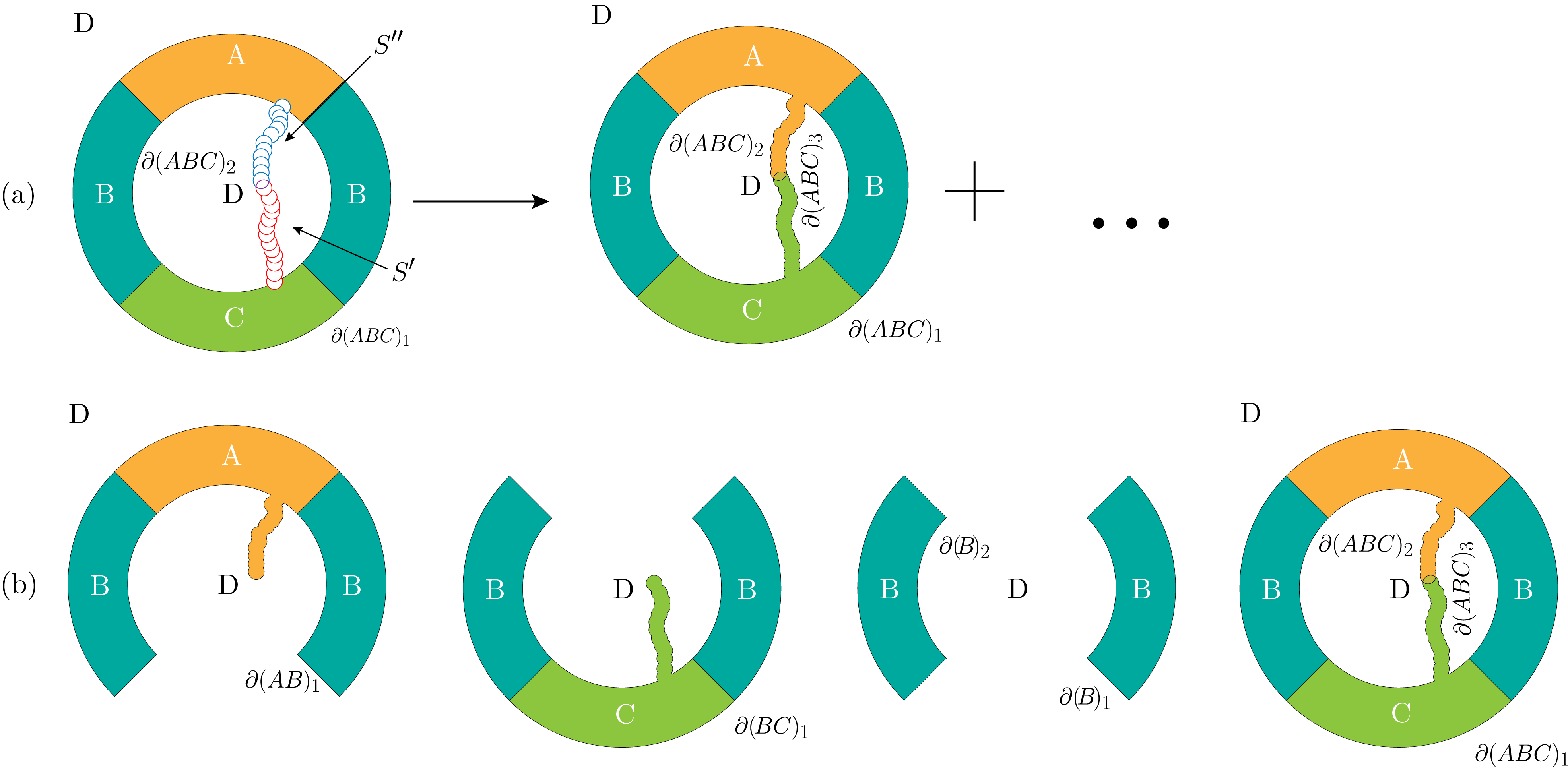
To prove the main theorem, we need to prove that, for any , the topological purity keeps the value of the topological purity of the initial state, i.e. the ratio of expectation values of evolved swap operators in Eq.(23) equals the ratio of expectation values of . In particular we consider two states, the ground state of the quantum double model and a topologically trivial state. If the initial state is the ground state of the quantum double model (cfr. Sec.1 ) then , while if the initial state is a pure and topologically trivial state such as , then .
Proof. Consider and let us compute the topological purity of for . According to Eq.(35) we can directly compute the expectation values of the evolution of the swap operators for . Recalling Eq.(33) the expectation value of the evolved swap operator is a linear combination of purities of in domains :
| (36) |
According to Eq. (7), any purity term , for equals to
| (37) |
where is the boundary length of and is the corresponding topological term. Then Eq.(35) can be expressed as
| (38) |
where we adopted a compact notation for the sum, namely etc. In order to illustrate how the previous relation works, let us first make a preliminary example and consider a single domain , so and , cfr. Sec.3.2; let be the domain sketched in Fig.8, i.e , we have:
| (39) |
the topological purity is given by their ratio:
| (40) |
where we used the following relations:
| (41) |
In fact, for any two terms and chosen from the denominator of Eq (38), one can always find two one-to-one corresponding terms and from the numerator, following the rule that the boundaries of them share the same trajectory of boundary statistic dynamics (see Fig 8 for the concrete rule).

As a consequence, it is not hard to find that the boundary length in purity expressions can cancel with each other , and the corresponding accumulative coefficients fulfill . In union with the fact that the topological terms keep the relation if since the perturbation can not cut apart the donut shape of system , we can reach the conclusion that
| (42) |
The proof for being a pure and topologically trivial state is identical to the one presented above, with the only difference that for any , cfr. Eq.(33). This concludes the proof.
Remark.
One wonders whether there are other boundary modifications that destroy the donut shape that can change the topological purity other than the one of conditions and . The answer is no: consider for example the ordered sets of domains and in Fig.9 . One of the result of their application is the boundary modification displayed in Fig.9 . Although it destroys the donut shape of it does not change the topological purity, indeed , , and therefore .

4 Conclusions
In this paper, we addressed some questions regarding the stability of topological order under noisy perturbations, but the path to find a general analytic proof is still long and tortuous. Working with the ground state of quantum double models, we defined a new detector for topological order - the topological purity - proving its robustness in two distinct phases, namely the topological phase and the trivial phase. More precisely, as a noise model, we introduced a set of quantum maps that mimics the evolution of local random quantum circuits. The two phases are indeed created by the quantum maps as orbits of two initially distinct states, the ground state of quantum double models and a pure, topologically trivial state. We found that the topological purity attains two different constant values among such states, in particular for the topologically ordered phase and for the trivial phase. The dynamics of the topological purity under such noise model can be mapped onto dynamics for the subsystems used to define the topological purity, cfr. Sec.2. This peculiarity enabled us to prove our main theorem and to provide many pictorial representations, giving the reader more intuition on the effects of the noisy dynamics. Despite the generality of the setup, our result is not the final word regarding the stability of topological order, and even more general and complete proofs are necessary to go further in this direction. This paper opens a series of different questions that might be interesting to investigate. Our proof strongly relies on the fact that the purity of the ground state of the quantum double model is a function of the boundary only: is this the case for other models and, more generally, is our proof working for any topologically ordered state? So far we only investigated the stability of topological purity, strictly related to the order two Rényi entropy: it would be indeed interesting to find an analytic treatment for more general detectors of topological order.
Acknowledgments
We acknowledge support from NSF award number 2014000.
References
- [1] X.-G. Wen, Quantum Field Theory of Many-Body Systems: From the Origin of Sound to an Origin of Light and Electrons, Oxford Graduate Texts. Oxford University Press, Oxford, ISBN 9780199227259, doi:10.1093/acprof:oso/9780199227259.001.0001 (2007).
- [2] A. Y. Kitaev, Fault-tolerant quantum computation by anyons, Annals of Physics 303(1), 2 (2003), doi:https://doi.org/10.1016/S0003-4916(02)00018-0.
- [3] M. H. Freedman, A. Kitaev et al., Topological quantum computation, Bulletin of the American Mathematical Society 40(01), 31 (2002), doi:10.1090/s0273-0979-02-00964-3.
- [4] A. Hamma, R. Ionicioiu and P. Zanardi, Ground state entanglement and geometric entropy in the kitaev model, Physics Letters A 337(1), 22 (2005), doi:https://doi.org/10.1016/j.physleta.2005.01.060.
- [5] A. Kitaev and J. Preskill, Topological entanglement entropy, Physical Review Letters 96, 110404 (2006), doi:10.1103/PhysRevLett.96.110404.
- [6] M. Levin and X.-G. Wen, Detecting topological order in a ground state wave function, Physical Review Letters 96, 110405 (2006), doi:10.1103/PhysRevLett.96.110405.
- [7] S. B. Chung, H. Yao et al., Topological quantum phase transition in an exactly solvable model of a chiral spin liquid at finite temperature, Physical Review B 81, 060403 (2010), doi:10.1103/PhysRevB.81.060403.
- [8] F. Mezzacapo, Ground-state phase diagram of the quantum model on the square lattice, Physical Review B 86, 045115 (2012), doi:10.1103/PhysRevB.86.045115.
- [9] S. Papanikolaou, K. S. Raman and E. Fradkin, Topological phases and topological entropy of two-dimensional systems with finite correlation length, Physical Review B 76, 224421 (2007), doi:10.1103/PhysRevB.76.224421.
- [10] Y. Zhang, T. Grover and A. Vishwanath, Topological entanglement entropy of spin liquids and lattice laughlin states, Physical Review B 84, 075128 (2011), doi:10.1103/PhysRevB.84.075128.
- [11] H.-C. Jiang, H. Yao and L. Balents, Spin liquid ground state of the spin- square - heisenberg model, Physical Review B 86, 024424 (2012), doi:10.1103/PhysRevB.86.024424.
- [12] H.-C. Jiang, Z. Wang and L. Balents, Identifying topological order by entanglement entropy, Nature Physics 8(12), 902–905 (2012), doi:10.1038/nphys2465.
- [13] S. Furukawa and G. Misguich, Topological entanglement entropy in the quantum dimer model on the triangular lattice, Physical Review B 75, 214407 (2007), doi:10.1103/PhysRevB.75.214407.
- [14] S. V. Isakov, M. B. Hastings and R. G. Melko, Topological entanglement entropy of a bose–hubbard spin liquid, Nature Physics 7(10), 772–775 (2011), doi:10.1038/nphys2036.
- [15] T. Micallo, V. Vitale et al., Topological entanglement properties of disconnected partitions in the Su-Schrieffer-Heeger model, SciPost Physics Core 3, 12 (2020), doi:10.21468/SciPostPhysCore.3.2.012.
- [16] S.-S. Gong, D. N. Sheng et al., Phase diagram of the spin- - heisenberg model on a honeycomb lattice, Physical Review B 88, 165138 (2013), doi:10.1103/PhysRevB.88.165138.
- [17] S. Dong, E. Fradkin et al., Topological entanglement entropy in chern-simons theories and quantum hall fluids, Journal of High Energy Physics 2008(05), 016–016 (2008), doi:10.1088/1126-6708/2008/05/016.
- [18] S. Trebst, P. Werner et al., Breakdown of a topological phase: Quantum phase transition in a loop gas model with tension, Physical Review Letters 98, 070602 (2007), doi:10.1103/PhysRevLett.98.070602.
- [19] A. Jamadagni, H. Weimer and A. Bhattacharyya, Robustness of topological order in the toric code with open boundaries, Physical Review B 98, 235147 (2018), doi:10.1103/PhysRevB.98.235147.
- [20] S. Dusuel, M. Kamfor et al., Robustness of a perturbed topological phase, Physical Review Letters 106, 107203 (2011), doi:10.1103/PhysRevLett.106.107203.
- [21] S. Bravyi, M. B. Hastings and S. Michalakis, Topological quantum order: Stability under local perturbations, Journal of Mathematical Physics 51(9), 093512 (2010), doi:10.1063/1.3490195.
- [22] S. Bravyi and M. B. Hastings, A short proof of stability of topological order under local perturbations, Communications in Mathematical Physics 307(3), 609 (2011), doi:10.1007/s00220-011-1346-2.
- [23] S. S. Jahromi, M. Kargarian et al., Robustness of a topological phase: Topological color code in a parallel magnetic field, Physical Review B 87, 094413 (2013), doi:10.1103/PhysRevB.87.094413.
- [24] A. Hamma, L. Cincio et al., Local response of topological order to an external perturbation, Physical Review Letters 110, 210602 (2013), doi:10.1103/PhysRevLett.110.210602.
- [25] S. Santra, A. Hamma et al., Local convertibility of the ground state of the perturbed toric code, Phys. Rev. B 90, 245128 (2014), doi:10.1103/PhysRevB.90.245128.
- [26] S. T. Flammia, A. Hamma et al., Topological entanglement rényi entropy and reduced density matrix structure, Physical Review Letters 103, 261601 (2009), doi:10.1103/PhysRevLett.103.261601.
- [27] L. Amico, R. Fazio et al., Entanglement in many-body systems, Reviews of Modern Physics 80, 517 (2008), doi:10.1103/RevModPhys.80.517.
- [28] P. Horodecki and A. Ekert, Method for direct detection of quantum entanglement, Physical Review Letters 89, 127902 (2002), doi:10.1103/PhysRevLett.89.127902.
- [29] M. B. Hastings, I. González et al., Measuring renyi entanglement entropy in quantum monte carlo simulations, Physical Review Letters 104, 157201 (2010), doi:10.1103/PhysRevLett.104.157201.
- [30] S. J. van Enk and C. W. J. Beenakker, Measuring on single copies of using random measurements, Physical Review Letters 108, 110503 (2012), doi:10.1103/PhysRevLett.108.110503.
- [31] D. A. Abanin and E. Demler, Measuring entanglement entropy of a generic many-body system with a quantum switch, Physical Review Letters 109, 020504 (2012), doi:10.1103/PhysRevLett.109.020504.
- [32] T. Brydges, A. Elben et al., Probing rényi entanglement entropy via randomized measurements, Science 364(6437), 260 (2019), doi:10.1126/science.aau4963,
- [33] P. Zanardi and L. Campos Venuti, Entanglement susceptibility: area laws and beyond, Journal of Statistical Mechanics: Theory and Experiment 2013(04), P04023 (2013), doi:10.1088/1742-5468/2013/04/p04023.
- [34] G. B. Halász and A. Hamma, Probing topological order with rényi entropy, Physical Review A 86, 062330 (2012), doi:10.1103/PhysRevA.86.062330.
- [35] D. N. Page, Average entropy of a subsystem, Physical Review Letters 71(9), 1291 (1993), doi:10.1103/physrevlett.71.1291.
- [36] S. Bose, I. Fuentes-Guridi et al., Subsystem purity as an enforcer of entanglement, Physical Review Letter 87, 050401 (2001), doi:10.1103/PhysRevLett.87.050401.
- [37] P. Zanardi and D. A. Lidar, Purity and state fidelity of quantum channels, Physical Review A 70, 012315 (2004), doi:10.1103/PhysRevA.70.012315.
- [38] D. Lidar, A. Shabani and R. Alicki, Conditions for strictly purity-decreasing quantum markovian dynamics, Chemical Physics 322(1), 82 (2006), doi:https://doi.org/10.1016/j.chemphys.2005.06.038, Real-time dynamics in complex quantum systems.
- [39] A. D. Pasquale, P. Facchi et al., Statistical distribution of the local purity in a large quantum system, Journal of Physics A: Mathematical and Theoretical 45(1), 015308 (2011), doi:10.1088/1751-8113/45/1/015308.
- [40] A. Streltsov, H. Kampermann et al., Maximal coherence and the resource theory of purity, New Journal of Physics 20(5), 053058 (2018), doi:10.1088/1367-2630/aac484.
- [41] M. A. Nielsen and I. L. Chuang, Quantum information theory, p. 528–607, Cambridge University Press, doi:10.1017/CBO9780511976667.016 (2010).
- [42] K. J. Satzinger, Y. Liu et al., Realizing topologically ordered states on a quantum processor, arXiv (2021), [quant-ph/2104.01180].
- [43] A. Hamma, S. Santra and P. Zanardi, Ensembles of physical states and random quantum circuits on graphs, Physical Review A 86, 052324 (2012), doi:10.1103/PhysRevA.86.052324.