Robust Generalization despite Distribution Shift via Minimum Discriminating Information

Developing machine learning-based systems for real world applications is challenging, particularly because the conditions under which the system was trained are rarely the same as when using the system. Unfortunately, a standard assumption in most machine learning methods is that test and training distribution are the same [78, 59, 12]. This assumption, however, rarely holds in practice, and the performance of many models suffers in light of this issue, often called dataset shift [52] or equivalently distribution shift. Consider building a model for diagnosing a specific heart disease, and suppose that most participants of the study are middle to high-aged men. Further suppose these participants have a higher risk for the specific disease, and as such do not reflect the general population with respect to age and gender. Consequently, the training data suffers from the so-called sample selection bias inducing a covariate shift [62, 52]. Many other reasons lead to distribution shifts, such as non-stationary environments [67], imbalanced data [52], domain shifts [3], label shifts [83] or observed contextual information [10, 11]. A specific type of distribution shift takes center stage in off-policy evaluation (OPE) problems. Here, one is concerned with the task of estimating the resulting cost of an evaluation policy for a sequential decision making problem based on historical data obtained from a different policy known as behavioral policy [73]. This problem is of critical importance in various applications of reinforcement learning—particularly, when it is impossible or unethical to evaluate the resulting cost of an evaluation policy by running it on the underlying system.
Solving a learning problem facing an arbitrary and unknown distribution shift based on training data in general is hopeless. Oftentimes, fortunately, partial knowledge about the distribution shift is available. In the medical example above, we might have prior information how the demographic attributes in our sample differ from the general population. Given a training distribution and partial knowledge about the shifted test distribution, one might ask what is the “most natural” distribution shift mapping the training distribution into a test distribution consistent with the available structural information. Here, we address this question, interpreting “most natural” as maximizing the underlying Shannon entropy. This concept has attracted significant interest in the past in its general form, called principle of minimum discriminating information dating back to Kullback [37], which can be seen as a generalization of Jaynes’ maximum entropy principle [31]. While these principles are widely used in tasks ranging from economics [27] to systems biology [63] and regularized Markov decision processes [48, 25, 2], they have not been investigated to model general distribution shifts as we consider in this paper.
Irrespective of the underlying distribution shift, the training distribution of any learning problem is rarely known, and one typically just has access to finitely many training samples. It is well-known that models can display a poor out-of-sample performance if training data is sparse. These overfitting effects are commonly avoided via regularization [12]. A regularization technique that has become popular in machine learning during the last decade and provably avoids overfitting is distributionally robust optimization (DRO) [36].

Contributions. We highlight the following main contributions of this paper:

• •

  We introduce a new modelling framework for distribution shifts via the principle of minimum discriminating information, which encodes prior structural information on the resulting test distribution.

• •

  Using our framework and the available training samples, we provide generalization bounds via a DRO program and prove that the introduced DRO model is optimal in a precise statistical sense.

• •

  We show that the optimization problems characterizing the distribution shift and the DRO program can be efficiently solved by exploiting convex duality and recent accelerated first order methods.

• •

  We demonstrate the versatility of the proposed Minimum Discriminating based DRO (MDI-DRO) method on two distinct problem classes: Training classifiers on systematically biased data and the OPE for Markov decision processes. In both problems MDI-DRO outperforms existing approaches.

The proofs of all technical results are relegated to Appendix 7.

For supervised learning problems, there is a rich literature in the context of covariate shift adaptation [62, 69]. A common approach is to address this distribution shift via importance sampling, more precisely by weighting the training loss with the ratio of the test and training densities and then minimize the so-called importance weighted risk (IWERM), see [62, 82, 69, 68]. While this importance weighted empirical risk is an unbiased estimator of the test risk, the method has two major limitations: It tends to produce an estimator with high variance, making the resulting test risk large. Further, the ratio of the training and test densities must be estimated which in general is difficult as the test distribution is unknown. There are modifications of IWERM reducing the resulting variance [15, 13, 65], for example by exponentially flattening the importance ratios [62]. For the estimation of the importance weights several methods have been presented, see for example [81]. These methods, however crucially rely on having data from both training and test distribution. [40] and [14] propose a minimax approach for regression problems under covariate shift. Similar to our approach taken in this paper, they consider a DRO framework, which however, optimizes over so-called moment-based ambiguity sets. Distribution shifts play a key role in causal inference. In particular, the connection between causal predictors and distributional robustness under shifts arising from interventions has been widely studied [58, 42, 56, 66]. Oftentimes, a causal graph is used to represent knowledge about the underlying distribution shift induced by an intervention [49, 50]. Distribution shifts have been addressed in a variety of different settings [35], we refer the reader to the comprehensive textbook [52] and references therein.
There is a vast literature on OPE methods which we will not attempt to summarize. In a nutshell, OPE methods can be grouped into three classes: a first class of approaches that aims to fit a model from the available data and uses this model then to estimate the performance of the given evaluation policy [41, 1, 38]. A second class of methods are based on invoking the idea of importance sampling to model the underlying distribution shift from behavioral to evaluation policy [51, 29, 74]. The third, more recent, class of methods combines the first two classes [24, 32, 76, 33].
Key reasons for the popularity of DRO in machine learning are the ability of DRO models to regularize learning problems [36, 61, 60] and the fact that the underlying optimization problems can often be exactly reformulated as finite convex programs solvable in polynomial time [4, 8]. Such reformulations hold for a variety of ambiguity sets such as: regions defined by moments [20, 26, 80, 9], $\phi$-divergences [5, 44, 39], Wasserstein ambiguity sets [43, 36], or maximum mean discrepancy ambiguity sets [64, 34]. DRO naturally seems a convenient tool when analyzing “small” distribution shifts as it seeks models that perform well “sufficiently close” to the training sample. However, modelling a general distribution shift via DRO seems difficult, and recent interest has focused on special cases such as adversarial example shifts [23] or label shifts [83]. To the best of our knowledge, the idea of combining DRO with the principle of minimum discriminating information is new.

We study learning problems of the form

where $R(\theta,\mathbb{P}^{\star})=\mathbb{E}_{\mathbb{P}^{\star}}[L(\theta,\xi)]$ denotes the risk of an uncertain real-valued loss function $L(\theta,\xi)$ that depends on a parameter $\theta\in\Theta\subset\mathbb{R}^{n}$ to be estimated as well as a random vector $\xi\in\Xi\subset\mathbb{R}^{m}$ governed by the probability distribution $\mathbb{P}^{\star}$. In order to avoid technicalities, we assume from now on that $\Theta$ and $\Xi$ are compact and $L$ is continuous. In statistical learning, it is usually assumed that $\mathbb{P}^{\star}$ is unknown but that we have access to independent samples from $\mathbb{P}^{\star}$. This paper departs from this standard scenario by assuming that there is a distribution shift. We first state our formal assumption about the shift and provide concrete examples below. Specifically, we assume to have access to samples from a distribution $\mathbb{P}\neq\mathbb{P}^{\star}$ and that $\mathbb{P}^{\star}$ is only known to belong to the distribution family

encoded by a measurable feature map $\psi:\Xi\to\mathbb{R}^{d}$ and a compact convex set $E\subset\mathbb{R}^{d}$. In view of the principle of minimum discriminating information, we identify $\mathbb{P}^{\star}$ with the I-projection of $\mathbb{P}$ onto $\Pi$.

One can show that the I-projection exists whenever $\Pi$ is closed with respect to the topology induced by the total variation distance [17, Theorem 2.1]. As $E$ is closed, this is the case whenever $\psi$ is bounded. Note that $f(\mathbb{P})=\mathbb{P}$ if $\mathbb{P}\in\Pi$. In the remainder, we assume that $\mathbb{P}\not\in\Pi$ and that $\mathbb{P}$ is only indirectly observable through independent training samples $\widehat{\xi}_{1},\ldots,\widehat{\xi}_{N}$ drawn from $\mathbb{P}$.

Loosely speaking, the principle of minimum discriminating information identifies the I-projection $\mathbb{P}^{f}$ of $\mathbb{P}$ as the least prejudiced and thus most natural model for $\mathbb{P}^{\star}$ in view of the information that $\mathbb{P}^{\star}\in\Pi$. The principle of minimum discriminating information is formally justified by the conditional limit theorem [18], which we paraphrase below using our notation.

In the context of Examples 3.1 and 3.2, the conditional limit theorem provides an intuitive justification for modeling distribution shifts via I-projections. More generally, the following proposition suggests that any distribution shift can be explained as an I-projection onto a suitably chosen set $\Pi$.

The modelling of arbitrary distribution shifts via the I-projection according to Proposition 3.2 has an interesting application in the off-policy evaluation problem for Markov decision processes (MDPs).

Given $N$ training samples $\widehat{\xi}_{1},\ldots,\widehat{\xi}_{N}$, we henceforth use $\widehat{\mathbb{P}}_{N}=\frac{1}{N}\sum_{i=1}^{N}\delta_{\widehat{\xi}_{i}}$ and $\widehat{\mathbb{P}}^{f}_{N}$ to denote the empirical distribution on and its I-projection onto $\Pi$, respectively. As the true data-generating distribution $\mathbb{P}$ and its I-projection $\mathbb{P}^{f}$ are unknown, it makes sense to replace them by their empirical counterparts. However, the resulting empirical risk minimization problem is susceptible to overfitting if the number of training samples is small relative to the feature dimension. In order to combat overfitting, we propose to solve the DRO problem

which minimizes the worst-case risk over all distributions close to $\widehat{\mathbb{P}}^{f}_{N}$. Here, $R^{\star}$ is defined through

and thus evaluates the worst-case risk of a given parameter $\theta\in\Theta$ in view of all distributions $\mathbb{Q}$ that have a relative entropy distance of at most $r$ from a given nominal distribution $\mathbb{P}^{\prime}\in\Pi$. In the remainder we use $J^{\star}_{N}$ and $\theta^{\star}_{N}$ to denote the minimum and a minimizer of problem (3.4), respectively.

Main results. The main theoretical results of this paper can be summarized as follows.

1. 1.

   Out-of-sample guarantee. We show that the optimal value of the DRO problem (3.4) provides an upper confidence bound on the risk of its optimal solution $\theta^{\star}_{N}$. Specifically, we prove that

   $\displaystyle\mathbb{P}^{N}\left(R(\theta^{\star}_{N},\mathbb{P}^{f})>J^{\star}_{N}\right)\leq e^{-rN+o(N)},$

   (3.6)

   where $\mathbb{P}^{f}=f(\mathbb{P})$ is the I-projection of $\mathbb{P}$. If $\Xi$ is finite, then (3.6) can be strengthened to a finite sample bound that holds for every $N$ if the right hand side is replaced with $e^{-rN}(N+1)^{|\Xi|}$.

2. 2.

   Statistical efficiency. In a sense to be made precise below, the DRO problem (3.4) provides the least conservative approximation for (3.1) whose solution satisfies the out-of-sample guarantee (3.6).

3. 3.

   Computational tractability. We prove that the I-projection $\widehat{\mathbb{P}}^{f}_{N}$ can be computed via a regularized fast gradient method whenever one can efficiently project onto $E$. Given $\widehat{\mathbb{P}}^{f}_{N}$, we then show that $\theta^{\star}_{N}$ can be found by solving a tractable convex program whenever $\Theta$ is a convex and conic representable set, while $L(\theta,\xi)$ is a convex and conic representable function of $\theta$ for any fixed $\xi$.

Throughout this section, we equip $\mathcal{P}(\Xi)$ with the topology of weak convergence. As $L(\theta,\xi)$ is continuous on $\Theta\times\Xi$ and $\Xi$ is compact, this implies that the risk $R(\theta,\mathbb{Q})$ is continuous on $\Theta\times\mathcal{P}(\Xi)$. The DRO problem (3.4) is constructed from the I-projection of the empirical distribution, which, in turn, is constructed from the given training samples. Thus, $\theta_{N}^{\star}$ constitutes a data-driven decision. Other data-driven decisions can be obtained by solving surrogate optimization problems of the form

where $\widehat{R}:\Theta\times\Pi\to\mathbb{R}$ is a continuous function that uses the empirical I-projection $\widehat{\mathbb{P}}^{f}_{N}$ to predict the true risk $R(\theta,\mathbb{P}^{f})$ of $\theta$ under the true I-projection $\mathbb{P}^{f}$. From now on we thus refer to $\widehat{R}$ as a predictor, and we use $\widehat{J}_{N}$ and $\widehat{\theta}_{N}$ to denote the minimum and a minimizer of problem (4.1), respectively. We call a predictor $\widehat{R}$ admissible if $\widehat{J}_{N}$ provides an upper confidence bound on the risk of $\widehat{\theta}_{N}$ in the sense that

for some prescribed $r>0$. The inequality (4.2) requires the true risk of the minimizer $\widehat{\theta}_{N}$ to exceed the optimal value $\widehat{J}_{N}$ of the surrogate optimization problem (4.1) with a probability that decays exponentially at rate $r$ as the number $N$ of training samples tends to infinity. The following theorem asserts that the DRO predictor $R^{\star}$ defined in (3.5), which evaluates the worst-case risk of any given $\theta$ across a relative entropy ball of radius $r$, almost satisfies (4.2) and is thus essentially admissible.

Theorem 4.1 implies that, for any fixed $\varepsilon>0$, the DRO predictor $R^{\star}$ provides an upper confidence bound $J^{\star}_{N}+\varepsilon$ on the true risk $R(\theta^{\star}_{N},\mathbb{P}^{f})$ of the data-driven decision $\theta^{\star}_{N}$ that becomes increasingly reliable as $N$ grows. Of course, the reliability of any upper confidence bound trivially improves if it is increased. Finding some upper confidence bound is thus easy. The next theorem shows that the DRO predictor actually provides the best possible (asymptotically smallest) upper confidence bound.

One readily verifies that the limits in Theorem 4.2 exist. Indeed, if $\widehat{R}$ is an arbitrary data-driven predictor, then the optimal value $\widehat{J}_{N}$ of the corresponding surrogate optimization problem converges $\mathbb{P}$-almost surely to $\min_{\theta\in\Theta}\widehat{R}(\theta,\mathbb{P}^{f})$ as $N$ tends infinity provided that the training samples are drawn independently from $\mathbb{P}$. This is a direct consequence of the following three observations. First, the optimal value function $\min_{\theta\in\Theta}\widehat{R}(\theta,\mathbb{P}^{f})$ is continuous in $\mathbb{P}^{f}\in\Pi$ thanks to Berge’s maximum theorem [7, pp. 115–116], which applies because $\widehat{R}$ is continuous and $\Theta$ is compact. Second, the I-projection $\mathbb{P}^{f}=f(\mathbb{P})$ is continuous in $\mathbb{P}\in\mathcal{P}(\Xi)$ thanks to [70, Theorem 9.17], which applies because the relative entropy is strictly convex in its first argument [21, Lemma 6.2.12]. Third, the strong law of large numbers implies that the empirical distribution $\widehat{\mathbb{P}}_{N}$ converges weakly to the data-generating distribution $\mathbb{P}$ as the sample size $N$ grows. Therefore, we have

In summary, Theorems 4.1 and 4.2 assert that the DRO predictor $R^{\star}$ is (essentially) admissible and that it is the least conservative of all admissible data-driven predictors, respectively. Put differently, the DRO predictor makes the most efficient use of the available data among all data-driven predictors that offer the same out-of-sample guarantee (4.2). In the special case when $\Xi$ is finite, the asymptotic out-of-sample guarantee (4.2) can be strengthened to a finite sample guarantee that holds for every $N\in\mathbb{N}$.

We now temporarily use $R^{\star}_{r}$ to denote the DRO predictor defined in (3.5), which makes its dependence on $r$ explicit. Note that if $r>0$ is kept constant, then $R_{r}^{\star}(\theta,\widehat{\mathbb{P}}_{N}^{f})$ is neither an unbiased nor a consistent estimator for $R(\theta,\mathbb{P}^{f})$. Consistency can be enforced, however, by shrinking $r$ as $N$ grows.

We now exemplify our DRO approach and its statistical guarantees in the context of the off-policy evaluation problem introduced in Section 3.

We now outline an efficient procedure to solve the DRO problem (3.4). This procedure consists of two steps. First, we propose an algorithm to compute the I-projection $\widehat{\mathbb{P}}^{f}_{N}=f(\widehat{\mathbb{P}}_{N})$ of the empirical distribution $\widehat{\mathbb{P}}_{N}$ corresponding to the training samples $\widehat{\xi}_{1},\ldots,\widehat{\xi}_{N}$. Given $\widehat{\mathbb{P}}^{f}_{N}$, we then show how to compute the worst-case risk $R^{\star}(\theta,\widehat{\mathbb{P}}_{N}^{f})$ and a corresponding optimizer $\theta^{\star}_{N}$ over the search space $\Theta$.

Computation of the I-projection. Computing the I-projection of the empirical distribution $\widehat{\mathbb{P}}_{N}$ is a non-trivial task because it requires solving the infinite-dimensional optimization problem (3.3). Generally, one would expect that the difficulty of evaluating $f(\widehat{\mathbb{P}}_{N})$ depends on the structure of the set $\Pi$, which is encoded by $\psi$ and $E$; see (3.2). Thanks to the discrete nature of the empirical distribution $\widehat{\mathbb{P}}_{N}$, however, we can leverage recent advances in convex optimization together with an algorithm proposed in [72] to show that $f(\widehat{\mathbb{P}}_{N})$ can be evaluated efficiently for a large class of sets $\Pi$.

In the following we let $\eta=(\eta_{1},\eta_{2})$ be a smoothing parameter with $\eta_{1},\eta_{2}>0$, and we let $L_{\eta}>0$ be a learning rate that may depend on $\eta$. In addition, we denote by $z\in\mathbb{R}^{d}$ the vector of dual variables of the constraint $\mathbb{E}_{\mathbb{Q}}[\psi(\xi)]\in E$ in problem (3.3), and we define $G_{\eta}:\mathbb{R}^{d}\to\mathbb{R}^{d}$ with

as a smoothed gradient of the dual objective, where $\pi_{E}$ denotes the projection operator onto $E$ defined through $\pi_{E}\left(z\right)=\arg\min_{x\in E}\|x-z\|_{2}^{2}$. The corresponding smoothed dual of the I-projection problem (3.3) can then be solved with the fast gradient method described in Algorithm 1. The complexity of evaluating $G_{\eta}$, and thus the per-iteration complexity of Algorithm 1, is determined by the projection operator onto $E$. For simple sets (e.g., 2-norm balls or hybercubes) the solution is available in closed form, and for many other sets (e.g., simplices or 1-norm balls) it can be computed cheaply, see [53, Section 5.4] for a comprehensive survey.

Any output $z_{k}$ of Algorithm 1 after $k$ iterations can be used to construct a candidate solution

for problem (3.3) that approximates the I-projection $\widehat{\mathbb{P}}^{f}_{N}$. The convergence guarantees for Algorithm 1 and, in particular, the approximation quality of (5.2) with respect to $\widehat{\mathbb{P}}^{f}_{N}$ detailed in Theorem 5.1 below require that problem (3.3) admits a Slater point $\mathbb{P}^{\circ}$ in the sense of the following assumption.

Finding a Slater point $\mathbb{P}^{\circ}$ may be difficult in general. However, $\mathbb{P}^{\circ}$ can be constructed systematically if $\psi$ is a polynomial [72, Remark 8], for example. Given $\mathbb{P}^{\circ}$ and a tolerance $\varepsilon>0$, we then define

Theorem 5.1 implies that Algorithm 1 needs at most $O(\frac{1}{\varepsilon}\log\frac{1}{\varepsilon})$ iterations to find an $O(\varepsilon)$-suboptimal and $O(\varepsilon)$-feasible solution for the I-projection problem (3.3). These results are derived via convex programming and duality by using the double smoothing techniques introduced in [22] and [72].

Computation of the DRO predictor. Equipped with Algorithm 1 to efficiently approximate $\widehat{\mathbb{P}}_{N}^{f}$ via $\widehat{\mathbb{Q}}_{k}$, the DRO predictor $R^{\star}(\theta,\widehat{\mathbb{P}}^{f}_{N})$ defined in (3.4) can be approximated by $R^{\star}(\theta,\widehat{\mathbb{Q}}_{k})$ because the function $R^{\star}$ is continuous. We now show that the worst-case risk evaluation problem (3.5) admits a dual representation, which generalizes [77, Proposition 5].

Proposition 5.1 implies that if $L(\theta,\xi)$ is convex in $\theta$ for every $\xi$, then the DRO predictor (3.5) coincides with the optimal value of a finite-dimensional convex program. Note that the objective function of (5.5) can be evaluated cheaply whenever the support function of $E$ is easy to compute and $\mathbb{P}^{\prime}$ has finite support (e.g., if $\mathbb{P}^{\prime}$ is set to an output $\widehat{\mathbb{Q}}_{k}$ of Algorithm 1). In addition, the robust constraint in (5.5) can be expressed in terms of explicit convex constraints if $L$, $\Xi$ and $\psi$ satisfy certain regularity conditions. A trivial condition is that $\Xi$ is finite. More general conditions are described in [6].

We now assess the empirical performance of the MDI-DRO method in our two running examples.¹¹ 1 All simulations were implemented in MATLAB and run on a 4GHz CPU with 16Gb RAM. The Matlab code for reproducing the plots is available from https://github.com/tobsutter/PMDI_DRO.

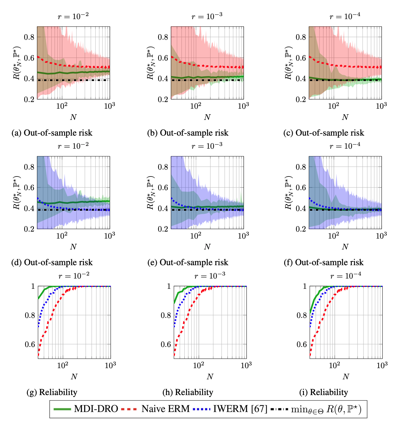
Synthetic dataset — covariate shift adaptation. The first two experiments revolve around the logistic regression problem with a distribution shift described in Example 3.1. Specifically, we consider a synthetic dataset where the test data is affected by a covariate shift, which constitutes a special case of a distribution shift. Detailed information about the data generation process is provided in Appendix 7.4. Our numerical experiments reveal that the proposed MDI-DRO method significantly outperforms the naive ERM method in the sense that its out-of-sample risk has both a lower mean as well as a lower variance; see Figures 1a and 1b. We also compare MDI-DRO against the IWERM method, which accounts for the distribution shift by assigning importance weights ${p^{\star}(\cdot)}/{p(\cdot)}$ to the training samples, where $p^{\star}(\cdot)$ and $p(\cdot)$ denote the densities of the test distribution $\mathbb{P}^{\star}$ and training distribution $\mathbb{P}$, respectively. These importance weights are assumed to be known in IWERM. In contrast, MDI-DRO does not require any knowledge of the test distribution other than its membership in $\Pi$. Nevertheless, MDI-DRO displays a similar out-of-sample performance as IWERM even though it has less information about $\mathbb{P}^{\star}$, and it achieves a lower variance than IWERM; see Figures 1c-1d. Figure 1e shows how the reliability of the upper confidence bound $J^{\star}_{N}$ and the out-of-sample risk $R(\theta^{\star}_{N},\mathbb{P}^{\star})$ change with the regularization parameter $r$. Additional results are reported in Figure 4 in the appendix. These results confirm that small regularization parameters $r$ lead to small out-of-sample risk and that increasing $r$ improves the reliability of the upper confidence bound $J^{\star}_{N}$.

Real data — classification under sample bias. The second experiment addresses the heart disease classification task of Example 3.1 based on a real dataset²² 2 https://www.kaggle.com/ronitf/heart-disease-uci consisting of $N^{\star}$ i.i.d. samples from an unknown test distribution $\mathbb{P}^{\star}$. To assess the effects of a distribution shift, we construct a biased training dataset $\{(\widehat{x}_{1},\widehat{y}_{1}),\ldots,(\widehat{x}_{N},\widehat{y}_{N})\}$, $N<N^{\star}$, in which male patients older than 60 years are substantially over-represented. Specifically, the $N$ training samples are drawn randomly from the set of the 20% oldest male patients. Thus, the training data follows a distribution $\mathbb{P}\neq\mathbb{P}^{\star}$. Even though the test distribution $\mathbb{P}^{\star}$ is unknown, we assume to know the empirical mean $m=\frac{1}{N^{\star}}\sum_{i=1}^{N^{\star}}(\widehat{x}_{i},\widehat{y}_{i})$ of the entire dataset to within an absolute error $\Delta m>0$. The test distribution thus belongs to the set $\Pi$ defined in (3.2) with $E=[m-\Delta m\mathsf{1},m+\Delta m\mathsf{1}]$ and with $\psi(x,y)=(x,y)$. We compare the proposed MDI-DRO method for classification against the naive ERM method that ignores the sample bias. In addition, we use a logistic regression model trained on the entire dataset as an (unachievable) ideal benchmark. Figure 2a shows the out-of-sample cost, Figure 2b the upper confidence bound $J^{\star}_{N}$ and Figure 2c the misclassification rates of the different methods as the radius $r$ of the ambiguity set is swept. Perhaps surprisingly, for some values of $r$ the classification performance of MDI-DRO is comparable to that of the logistic regression method trained on the entire dataset.

OPE for MDPs — inventory control. We now consider the OPE problem of Examples 3.3 and 4.1. A popular estimator for the cost $V_{\pi_{\mathsf{e}}}$ of the evaluation policy is the inverse propensity score (IPS) [57]

Hoeffding’s inequality then gives rise to the simple concentration bound

where $b=\max_{s\in\mathcal{S},a\in\mathcal{A}}c(s,a)\mu_{\mathsf{e}}(s,a)/\mu_{\mathsf{b}}(s,a)$. As $b$ is typically a large constant, the finite sample bound (4.5) for $J^{\star}_{N}$ is often more informative than (6.1). In addition, the variance of $\widehat{J}_{N}^{\rm IPS}$ grows exponentially with the sample size $N$ [15, 13, 65]. As a simple remedy, one can cap the importance weights beyond some threshold $\beta>0$ and construct the modified IPS estimator as

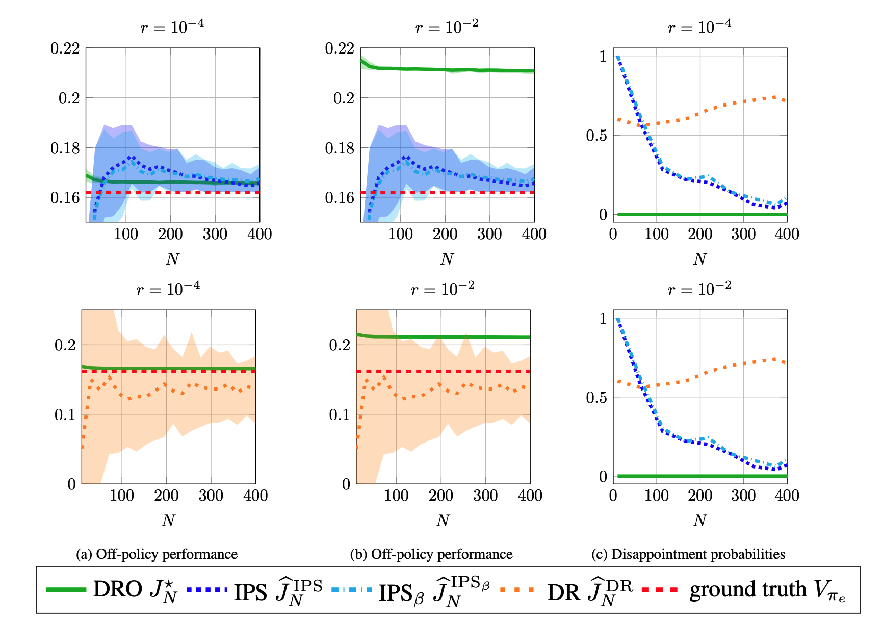
Decreasing $\beta$ reduces the variance of $\widehat{J}_{N}^{\mathop{\rm IPS}_{\beta}}$ but increases its bias. An alternative estimator for $V_{\pi_{\mathsf{e}}}$ is the doubly robust (DR) estimator $\widehat{J}_{N}^{\rm DR}$, which uses a control variate to reduce the variance of the IPS estimator. The DR estimator was first developed for contextual bandits [24] and then generalized to MDPs [32, 75]. We evaluate the performance of the proposed MDI-DRO estimator on a classical inventory control problem. A detailed problem description is relegated to Appendix 7.4. We sample both the evaluation policy $\pi_{\mathsf{e}}$ and the behavioral policy $\pi_{\mathsf{b}}$ from the uniform distribution on the space of stationary policies. The decision maker then has access to the evaluation policy $\pi_{\mathsf{e}}$ and to a sequence of i.i.d. state action pairs $\{\widehat{s}_{i},\widehat{a}_{i}\}_{i=1}^{N}$ sampled from $\mu_{\mathsf{b}}$ as well as the observed empirical costs $\{\widehat{c}_{i}\}_{i=1}^{N}$, where $\widehat{c}_{i}=c(\widehat{s}_{i},\widehat{a}_{i})$. Figure 3 compares the proposed MDI-DRO estimator against the original and modified IPS estimators, the DR estimator and the ground truth expected cost of the evaluation policy. Figures 3a and 3b show that for small radii $r$, the MDI-DRO estimator outperforms the IPS estimators both in terms of accuracy and precision. Figure 3c displays the disappointment probabilities $\mathbb{P}^{N}(V_{\pi_{\mathsf{e}}}>\widehat{J}_{N})$ analyzed in Theorem 4.1, where $\widehat{J}_{N}$ denotes any of the tested estimators.

Acknowledgments. This research was supported by the Swiss National Science Foundation under the NCCR Automation, grant agreement 51NF40_180545.

The appendix details all proofs and provides some auxiliary results grouped by section.

References

- [1] András Antos, Csaba Szepesvári, and Rémi Munos. Learning near-optimal policies with Bellman-residual minimization based fitted policy iteration and a single sample path. In Learning Theory, pages 574–588. Springer, 2006.
- [2] Boris Belousov and Jan Peters. Entropic regularization of Markov decision processes. Entropy, 21(7), 2019.
- [3] Shai Ben-David, John Blitzer, Koby Crammer, and Fernando Pereira. Analysis of representations for domain adaptation. In Advances in Neural Information Processing Systems, 2007.
- [4] A. Ben-Tal, L. El Ghaoui, and A. Nemirovski. Robust Optimization. Princeton University Press, 2009.
- [5] Aharon Ben-Tal, Dick den Hertog, Anja De Waegenaere, Bertrand Melenberg, and Gijs Rennen. Robust solutions of optimization problems affected by uncertain probabilities. Management Science, 59(2):341–357, 2013.
- [6] Aharon Ben-Tal, Dick den Hertog, and Jean-Philippe Vial. Deriving robust counterparts of nonlinear uncertain inequalities. Mathematical Programming, 149(1):265–299, 2015.
- [7] Claude Berge. Topological Spaces: Including a Treatment of Multi-valued Functions, Vector Spaces, and Convexity. Courier Corporation, 1997.
- [8] D. Bertsimas and M. Sim. The price of robustness. Operations Research, 52(1):35–53, 2004.
- [9] Dimitris Bertsimas, Vishal Gupta, and Nathan Kallus. Data-driven robust optimization. Mathematical Programming, 167(2):235–292, 2018.
- [10] Dimitris Bertsimas and Nathan Kallus. From predictive to prescriptive analytics. Management Science, 66(3):1025–1044, 2020.
- [11] Dimitris Bertsimas and Bart Van Parys. Bootstrap robust prescriptive analytics. arXiv preprint arXiv:1711.09974, Accepted in Mathematical Programming, 2017.
- [12] Christopher M. Bishop. Pattern Recognition and Machine Learning. Springer, 2006.
- [13] Léon Bottou, Jonas Peters, Joaquin Quiñonero-Candela, Denis X. Charles, D. Max Chickering, Elon Portugaly, Dipankar Ray, Patrice Simard, and Ed Snelson. Counterfactual reasoning and learning systems: The example of computational advertising. Journal of Machine Learning Research, 14(65):3207–3260, 2013.
- [14] Xiangli Chen, Mathew Monfort, Anqi Liu, and Brian D. Ziebart. Robust covariate shift regression. In International Conference on Artificial Intelligence and Statistics, 2016.
- [15] Corinna Cortes, Yishay Mansour, and Mehryar Mohri. Learning bounds for importance weighting. In Advances in Neural Information Processing Systems, 2010.
- [16] T.M. Cover and J.A. Thomas. Elements of Information Theory. Wiley, 2006.
- [17] I. Csiszár. I-divergence geometry of probability distributions and minimization problems. Annals of Probability, 3(1):146–158, 02 1975.
- [18] Imre Csiszár. Sanov property, generalized -projection and a conditional limit theorem. The Annals of Probability, 12(3):768–793, 1984.
- [19] Imre Csiszár and Janos Korner. Information Theory: Coding Theorems for Discrete Memoryless Systems. Academic Press, 1982.
- [20] E. Delage and Y. Ye. Distributionally robust optimization under moment uncertainty with application to data-driven problems. Operations Research, 58(3):595–612, 2010.
- [21] A. Dembo and O. Zeitouni. Large Deviations Techniques and Applications. Springer, 2009.
- [22] Olivier Devolder, François Glineur, and Yurii Nesterov. Double smoothing technique for large-scale linearly constrained convex optimization. SIAM Journal on Optimization, 22(2):702–727, 2012.
- [23] John Duchi and Hongseok Namkoong. Learning models with uniform performance via distributionally robust optimization. arXiv preprint, arXiv.1810.08750, Accepted in Annals of Statistics, 2020.
- [24] Miroslav Dudik, Dumitru Erhan, John Langford, and Lihong Li. Doubly Robust Policy Evaluation and Optimization. Statistical Science, 29(4):485–511, 2014.
- [25] Matthieu Geist, Bruno Scherrer, and Olivier Pietquin. A theory of regularized Markov decision processes. In International Conference on Machine Learning, 2019.
- [26] J. Goh and M. Sim. Distributionally robust optimization and its tractable approximations. Operations Research, 58(4):902–917, 2010.
- [27] Amos Golan. Information and Entropy Econometrics: Review and Synthesis. Foundations and Trends in Econometrics, 2(1-2):1–145, 2008.
- [28] O. Hernández-Lerma and J.B. Lasserre. Discrete-Time Markov Control Processes: Basic Optimality Criteria. Springer, 1996.
- [29] Keisuke Hirano, Guido W. Imbens, and Geert Ridder. Efficient estimation of average treatment effects using the estimated propensity score. Econometrica, 71(4):1161–1189, 2003.
- [30] Joseph Horowitz and Rajeeva L. Karandikar. Mean rates of convergence of empirical measures in the Wasserstein metric. Journal of Computational and Applied Mathematics, 55(3):261–273, 1994.
- [31] Edwin T. Jaynes. Information theory and statistical mechanics. Physical Review, 108:171–190, 1957.
- [32] Nan Jiang and Lihong Li. Doubly robust off-policy value evaluation for reinforcement learning. In International Conference on Machine Learning, 2016.
- [33] Nathan Kallus and Masatoshi Uehara. Double reinforcement learning for efficient off-policy evaluation in Markov decision processes. Journal of Machine Learning Research, 21(167):1–63, 2020.
- [34] Johannes Kirschner, Ilija Bogunovic, Stefanie Jegelka, and Andreas Krause. Distributionally robust Bayesian optimization. In Artificial Intelligence and Statistics, 2020.
- [35] Kun Kuang, Peng Cui, Susan Athey, Ruoxuan Xiong, and Bo Li. Stable prediction across unknown environments. In International Conference on Knowledge Discovery & Data Mining, 2018.
- [36] Daniel Kuhn, Peyman Mohajerin Esfahani, Viet Anh Nguyen, and Soroosh Shafieezadeh Abadeh. Wasserstein distributionally robust optimization: Theory and applications in machine learning. INFORMS TutORials in Operations Research, pages 130–166, 2019.
- [37] S. Kullback. Information Theory and Statistics. Wiley, 1959.
- [38] Michail G. Lagoudakis and Ronald Parr. Least-squares policy iteration. Journal on Machine Learning Research, 4:1107–1149, 2003.
- [39] Mengmeng Li, Tobias Sutter, and Daniel Kuhn. Distributionally robust optimization with Markovian data. In International Conference on Machine Learning, 2021.
- [40] Anqi Liu and Brian Ziebart. Robust classification under sample selection bias. In Advances in Neural Information Processing Systems, 2014.
- [41] Shie Mannor, Duncan Simester, Peng Sun, and John N. Tsitsiklis. Bias and variance approximation in value function estimates. Management Science, 53(2):308–322, 2007.
- [42] Nicolai Meinshausen. Causality from a distributional robustness point of view. In IEEE Data Science Workshop (DSW), 2018.
- [43] Peyman Mohajerin Esfahani and Daniel Kuhn. Data-driven distributionally robust optimization using the Wasserstein metric: Performance guarantees and tractable reformulations. Mathematical Programming, 171(1-2):115–166, 2018.
- [44] Hongseok Namkoong and John C Duchi. Stochastic gradient methods for distributionally robust optimization with f-divergences. In Advances in Neural Information Processing Systems, 2016.
- [45] Angelia Nedić and Asuman Ozdaglar. Approximate primal solutions and rate analysis for dual subgradient methods. SIAM Journal on Optimization, 19(4):1757–1780, 2008.
- [46] Yurii Nesterov. Smooth minimization of non-smooth functions. Mathematical Programming, 103(1):127–152, 2005.
- [47] Yurii Nesterov. Introductory Lectures on Convex Optimization: A Basic Course. Springer, 2014.
- [48] Gergely Neu, Anders Jonsson, and Vicenç Gómez. A unified view of entropy-regularized Markov decision processes. arXiv preprint arXiv:1705.07798, 2017.
- [49] Judea Pearl and Elias Bareinboim. Transportability of causal and statistical relations: A formal approach. In IEEE International Conference on Data Mining Workshops, 2011.
- [50] Jonas Peters, Dominik Janzing, and Bernhard Schölkopf. Elements of Causal Inference: Foundations and Learning Algorithms. MIT Press, 2017.
- [51] Doina Precup, Richard S. Sutton, and Satinder P. Singh. Eligibility traces for off-policy policy evaluation. In International Conference on Machine Learning, 2000.
- [52] Joaquin Quionero-Candela, Masashi Sugiyama, Anton Schwaighofer, and Neil D. Lawrence. Dataset Shift in Machine Learning. MIT Press, 2009.
- [53] S. Richter. Computational Complexity Certification of Gradient Methods for Real-Time Model Predictive Control. PhD thesis, ETH Zurich, 2012.
- [54] R. Tyrrell Rockafellar. Convex Analysis. Princeton University Press, 1997.
- [55] R. Tyrrell Rockafellar and Roger Jean-Baptiste Wets. Variational Analysis. Springer, 1998.
- [56] Mateo Rojas-Carulla, Bernhard Schölkopf, Richard Turner, and Jonas Peters. Invariant models for causal transfer learning. Journal of Machine Learning Research, 19(36):1–34, 2018.
- [57] Paul R. Rosenbaum and Donald B. Rubin. The central role of the propensity score in observational studies for causal effects. Biometrika, 70(1):41–55, 1983.
- [58] Dominik Rothenhäusler, Peter Bühlmann, Nicolai Meinshausen, and Jonas Peters. Anchor regression: Heterogeneous data meet causality. Journal of the Royal Statistical Society: Series B, 83(2):215–246, 2021.
- [59] Bernhard Schölkopf and Alexander J. Smola. Learning with Kernels: Support Vector Machines, Regularization, Optimization, and Beyond. MIT Press, 2001.
- [60] Soroosh Shafieezadeh-Abadeh, Daniel Kuhn, and Peyman Mohajerin Esfahani. Regularization via mass transportation. Journal of Machine Learning Research, 20(103):1–68, 2019.
- [61] Soroosh Shafieezadeh Abadeh, Peyman Mohajerin Esfahani, and Daniel Kuhn. Distributionally robust logistic regression. In Advances in Neural Information Processing Systems, 2015.
- [62] Hidetoshi Shimodaira. Improving predictive inference under covariate shift by weighting the log-likelihood function. Journal of Statistical Planning and Inference, 90(2):227–244, 2000.
- [63] Patrick Smadbeck and Yiannis N. Kaznessis. On a theory of stability for nonlinear stochastic chemical reaction networks. The Journal of Chemical Physics, 142(18), 2015.
- [64] Matthew Staib and Stefanie Jegelka. Distributionally robust optimization and generalization in kernel methods. In Advances in Neural Information Processing Systems, 2019.
- [65] Alexander L. Strehl, John Langford, Lihong Li, and Sham M. Kakade. Learning from logged implicit exploration data. In Advances in Neural Information Processing Systems, pages 2217–2225, 2010.
- [66] Adarsh Subbaswamy, Peter Schulam, and Suchi Saria. Preventing failures due to dataset shift: Learning predictive models that transport. In International Conference on Artificial Intelligence and Statistics, 2019.
- [67] Masashi Sugiyama and Motoaki Kawanabe. Machine Learning in Non-Stationary Environments: Introduction to Covariate Shift Adaptation. MIT Press, 2012.
- [68] Masashi Sugiyama, Matthias Krauledat, and Klaus-Robert Müller. Covariate shift adaptation by importance weighted cross validation. Journal of Machine Learning Research, 8(35):985–1005, 2007.
- [69] Masashi Sugiyama and Klaus-Robert Müller. Input-dependent estimation of generalization error under covariate shift. Statistics & Decisions, 23:249–279, 2005.
- [70] Rangarajan K. Sundaram. A First Course in Optimization Theory. Cambridge University Press, 1996.
- [71] Tobias Sutter, Bart P. G. Van Parys, and Daniel Kuhn. A general framework for optimal data-driven optimization. arXiv preprint, 2010.06606, 2020.
- [72] Tobias Sutter, David Sutter, Peyman Mohajerin Esfahani, and John Lygeros. Generalized maximum entropy estimation. Journal of Machine Learning Research, 20(138):1–29, 2019.
- [73] Richard S. Sutton and Andrew G. Barto. Reinforcement Learning: An Introduction. MIT Press, 2018.
- [74] Adith Swaminathan and Thorsten Joachims. The self-normalized estimator for counterfactual learning. In Advances in Neural Information Processing Systems, 2015.
- [75] Ziyang Tang, Yihao Feng, Lihong Li, Dengyong Zhou, and Qiang Liu. Doubly robust bias reduction in infinite horizon off-policy estimation. In International Conference on Learning Representations, 2020.
- [76] Philip Thomas and Emma Brunskill. Data-efficient off-policy policy evaluation for reinforcement learning. In International Conference on Machine Learning, 2016.
- [77] Bart Van Parys, Peyman Mohajerin Esfahani, and Daniel Kuhn. From data to decisions: Distributionally robust optimization is optimal. Management Science, 67(6):3387–3402, 2021.
- [78] V.N. Vapnik. Statistical Learning Theory. Wiley, 1998.
- [79] C. Villani. Optimal Transport: Old and New. Springer, 2008.
- [80] W. Wiesemann, D. Kuhn, and M. Sim. Distributionally robust convex optimization. Operations Research, 62(6):1358–1376, 2014.
- [81] Makoto Yamada, Taiji Suzuki, Takafumi Kanamori, Hirotaka Hachiya, and Masashi Sugiyama. Relative density-ratio estimation for robust distribution comparison. In Advances in Neural Information Processing Systems, 2011.
- [82] Bianca Zadrozny. Learning and evaluating classifiers under sample selection bias. In International Conference on Machine Learning, 2004.
- [83] Jingzhao Zhang, Aditya Menon, Andreas Veit, Srinadh Bhojanapalli, Sanjiv Kumar, and Suvrit Sra. Coping with label shift via distributionally robust optimisation. arXiv preprint, arXiv.2010.12230, 2020.