Spreading properties for SIR models on homogeneous trees

We complement (1.2) with an initial condition of the form

$$S_{j}(t=0)=s_{0},\quad I_{j}(t=0)=I_{j}^{0},\quad j\in\mathbb{Z},$$

(2.1)

where $s_{0}\in(0,1)$ and $I_{j}^{0}\in(0,1)$ for each $j\in\mathbb{Z}$ has finite support. As already stated in the introduction, our aim is to investigate the long time dynamics of (1.2) subject to the initial condition (2.1). We define the cumulative density of infected individuals at lattice site $j$ and time $t$ as $\mathcal{I}_{j}(t):=\int_{0}^{t}I_{j}(s)\mathrm{d}s$ such that the density of susceptible individuals can be expressed as

$$\ln\left(\frac{S_{j}(t)}{s_{0}}\right)=-\tau\mathcal{I}_{j}(t).$$

Thus $\mathcal{I}_{j}(t)$ satisfies the lattice differential equation

$$\mathcal{I}_{j}^{\prime}(t)=f(\mathcal{I}_{j}(t))+I_{j}^{0}+\lambda\left(\mathcal{I}_{j-1}(t)-2\mathcal{I}_{j}(t)+\mathcal{I}_{j+1}(t)\right),$$

(2.2)

together with the initial condition

$$\mathcal{I}_{j}(t=0)=0,\quad\text{ for all }\quad j\in\mathbb{Z}.$$

(2.3)

Here, the nonlinearity $f$ is given by

$$f(v):=s_{0}\left(1-e^{-\tau v}\right)-\eta v,$$

which is smooth, concave on $[0,+\infty)$ and vanishes at $v=0$. For future reference, we note that

$$f^{\prime}(0)=\eta\left(\mathscr{R}_{0}-1\right),\quad\mathscr{R}_{0}:=\frac{s_{0}\tau}{\eta}.$$

The quantity $\mathscr{R}_{0}$ is the usual basic reproduction number [18, 29]. Our first result states the existence of a unique positive, bounded, stationary solution to (2.2) and characterizes its asymptotic behavior, see Figure 2 for an illustration.

It is interesting to point out that (2.2) can be interpreted as a reaction-diffusion equation of Fisher-KPP type on the lattice $\mathbb{Z}$ with a heterogeneity given by $I_{j}^{0}$. We refer to [11, 23] for spreading properties of the Fisher-KPP equation set on the lattice $\mathbb{Z}$. In our SIR epidemic setting, as in the continuous case [3], it turns out that the above stationary solution is a global attractor for the dynamics of (2.2) which is the result of the following theorem.

A consequence of the above Theorem 2 is that the convergence also holds true for the time derivative of $\left(\mathcal{I}_{j}(t)\right)_{j\in\mathbb{Z}}$ such that we can deduce that locally uniformly in $j$ we have

$$I_{j}(t)=\mathcal{I}_{j}^{\prime}(t)\rightarrow 0\text{ as }t\rightarrow+\infty,$$

which means that the density of infected individuals asymptotically vanishes in time at each fixed lattice site. Recalling that the density of susceptible individuals can be read out from $\mathcal{I}_{j}(t)$ via

$$S_{j}(t)=s_{0}e^{-\tau\mathcal{I}_{j}(t)},$$

we can also quantify the density of individuals that will be infected during the course of the epidemic at a given lattice site $j$, that we denote $\mathcal{I}_{j}^{tot}$. It is given by

$$\mathcal{I}_{j}^{tot}=s_{0}\left(1-e^{-\tau\mathcal{I}_{j}^{\infty}}\right),\quad j\in\mathbb{Z}.$$

As in the fully continuous setting [19, 3], we remark that $\left(\mathcal{I}_{j}^{tot}\right)_{j\in\mathbb{Z}}$ is not constant, which comes from our assumption that susceptible individuals do not diffuse on the lattice. Now, using the result of Theorem 1, we obtain the following dichotomy

$$\underset{|j|\rightarrow+\infty}{\lim}\mathcal{I}_{j}^{tot}=\left\{\begin{array}[]{lcl}0,&\text{if}&\mathscr{R}_{0}\leq 1,\\ s_{0}\left(1-e^{-\tau\mathcal{I}_{*}}\right),&\text{if}&\mathscr{R}_{0}>1.\end{array}\right.$$

This basically says that when $\mathscr{R}_{0}\leq 1$ the epidemic does not propagate across the network and lattice sites very far from the support of the initial condition will effectively be not infected. On the other hand, when the basic reproduction number verifies $\mathscr{R}_{0}>1$, the epidemic propagates everywhere across the lattice. Very far from the support of the initial condition, there will be a portion $1-e^{-\tau\mathcal{I}_{*}}$ of infected individuals of the overall population. When $\mathscr{R}_{0}>1$, we can further characterize at which speed the epidemic spreads into the lattice and this is precisely the result of the next theorem.

The quantity $c_{*}$ is the asymptotic speed of spreading of the epidemic wave and it coincides with the asymptotic speed of spreading for the Fisher-KPP equation set on the lattice [23]. As already noticed in [23], we have the following asymptotic of the spreading speed $c_{*}$ when $\lambda$ is small

$$c_{*}\sim W_{0}\left(\frac{\eta(\mathscr{R}_{0}-1)}{\lambda}\right)\text{ as }\lambda\rightarrow 0,$$

where $W_{0}$ denotes the principal branch of the Lambert W function, that is the multivalued inverse relation of the function $f(w)=we^{w}$ for $w\in\mathbb{C}$ [17]. On the other hand, when $\lambda$ is large, we have that

$$c_{*}\sim 2\sqrt{\eta(\mathscr{R}_{0}-1)\lambda}\text{ as }\lambda\rightarrow+\infty.$$

Let us remark that $2\sqrt{\eta(\mathscr{R}_{0}-1)\lambda}$ is precisely the asymptotic speed of propagation in the continuous case [3]. It turns out that the speed $c_{*}$ also characterizes the threshold for the existence of traveling wave solutions associated to system (1.2). For a given $s_{0}\in(0,1)$, by traveling wave solution to system (1.2) we mean a solution of (1.2) which takes the form $(S_{j}(t),I_{j}(t))=(S(j-ct),I(j-ct))$ with profiles $(S(x),I(x))$ and wave speed $c$ solutions of

$$\left\{\begin{split}-cS^{\prime}(x)&=-\tau S(x)I(x),\\ -cI^{\prime}(x)&=\tau S(x)I(x)-\eta I(x)+\lambda\left(I(x-1)-2I(x)+I(x+1)\right),\\ c>0,&\quad I>0\text{ is bounded },\quad 0<S<s_{0},\end{split}\right.$$

(2.4)

with asymptotic conditions

$$\left\{\begin{split}S(+\infty)&=s_{0},\\ I(\pm\infty)&=0.\end{split}\right.$$

(2.5)

Here the wave speed $c>0$ is to be determined and we do not impose a prescribed value for $S$ at $-\infty$.

Existence and uniqueness results of traveling wave solutions for discrete epidemic models on a lattice have been obtained recently [20, 31, 15], but not directly for system (2.4). Indeed, in [20, 31, 15], the density of susceptible individuals is also subject to discrete diffusion which prevents us to directly apply to our system the aforementioned results. Nevertheless, we can easily notice that system (2.4)-(2.5) can be recast as a traveling wave problem for the discrete Fisher-KPP problem by introducing $\mathcal{I}(x):=\frac{1}{c}\int_{x}^{+\infty}I(z)\mathrm{d}z$ for which existence and uniqueness results are readily available [32, 13, 14].

We now turn our attention to the case where our epidemic model (1.1) is set on a homogeneous tree of degree $k\geq 2$. Throughout this section, we will assume that the initial density of infected individuals is non zero at only one vertex of the graph. We recall from the introduction that we label this vertex as $1$ and denote $(S_{1}(t),I_{1}(t))$ the associated density. Using the symmetry of the model, we also denote $(S_{n}(t),I_{n}(t))$ a representative vertex from the set of vertices at distance $n-1$ from the root. As a consequence, the sequence $(S_{n}(t),I_{n}(t))_{n\geq 1}$ is solution of the system (1.4)-(1.5) which is complemented with an initial of the form

$$S_{n}(t=0)=s_{0},\quad n\geq 1,\quad I_{1}(t=0)=i_{0},\quad I_{n}(t=0)=0,\quad n\geq 2,$$

for some $s_{0}\in(0,1)$ and $i_{0}\in(0,1)$. We refer to Figure 4 for an illustration of the configuration of the initial condition for the density of infected individuals in the case $k=2$.

Once again, for each $n\geq 1$, we define the cumulated density of infected individuals as $\mathcal{I}_{n}(t):=\int_{0}^{t}I_{n}(s)\mathrm{d}s$ which satisfies

$$\left\{\begin{split}\mathcal{I}^{\prime}_{n}(t)&=f(\mathcal{I}_{n}(t))+\lambda\left(\mathcal{I}_{n-1}(t)-(k+1)\mathcal{I}_{n}(t)+k\mathcal{I}_{n+1}(t)\right),\quad n\geq 2,\\ \mathcal{I}^{\prime}_{1}(t)&=f(\mathcal{I}_{1}(t))+i_{0}+\lambda(k+1)\left(-\mathcal{I}_{1}(t)+\mathcal{I}_{2}(t)\right),\end{split}\right.$$

(2.6)

together with the initial condition

$$\mathcal{I}_{n}(t=0)=0,\quad\text{ for all }\quad n\geq 1.$$

(2.7)

We start by studying stationary solutions to (2.6), and as in Theorem 1 on the lattice, we have existence and uniqueness of a positive bounded stationary solution. Similarly, when the basic reproduction number satisfies $\mathscr{R}_{0}\leq 1$, the stationary solution $\mathcal{I}_{n}^{\infty}$ converges to zero as $n$ goes to infinity.

It turns out that the asymptotic behavior of the stationary solution when $\mathscr{R}_{0}>1$ is more intricate than in the case on the lattice. We have the following result.

We remark that there is a threshold on the parameter $\lambda$, which depends on the degree $k$ of the homogeneous tree and the basic reproduction number $\mathscr{R}_{0}$, below which the stationary solution asymptotically converges to $\mathcal{I}_{*}>0$ the unique positive zero of $f$ and above which it asymptotically converges to zero. Let us heuristically explain how this critical value emerges. For $n\geq 2$, stationary solutions satisfy

$$0=f(\mathcal{I}_{n}^{\infty})+\lambda\left(\mathcal{I}_{n-1}^{\infty}-(k+1)\mathcal{I}_{n}^{\infty}+k\mathcal{I}_{n+1}^{\infty}\right),$$

and one can look for exponential supersolutions of the form $\overline{\mathcal{I}}_{n}^{\infty}=Ce^{-\gamma n}$ for some well chosen constant $C>0$ and $\gamma>0$. Using the concavity of $f$, we get that

$$f(\overline{\mathcal{I}}_{n}^{\infty})+\lambda\left(\overline{\mathcal{I}}_{n-1}^{\infty}-(k+1)\overline{\mathcal{I}}_{n}^{\infty}+k\overline{\mathcal{I}}_{n+1}^{\infty}\right)<\left(\eta(\mathscr{R}_{0}-1)+\lambda\left(e^{\gamma}-(k+1)+ke^{-\gamma}\right)\right)Ce^{-\gamma n},$$

and we denote

$$\mathcal{D}(\gamma):=\eta(\mathscr{R}_{0}-1)+\lambda\left(e^{\gamma}-(k+1)+ke^{-\gamma}\right).$$

We readily remark that $\mathcal{D}$ is convex with $\mathcal{D}(0)=\eta(\mathscr{R}_{0}-1)>0$ and $\mathcal{D}(+\infty)=+\infty$. Furthermore, $\mathcal{D}^{\prime}(\gamma)=0$ if and only if $\gamma=\ln\sqrt{k}$, and we note that

$$\mathcal{D}(\ln\sqrt{k})=\eta(\mathscr{R}_{0}-1)-\lambda(k+1-2\sqrt{k})=(k+1-2\sqrt{k})(\lambda_{c}-\lambda).$$

As a consequence, when $\lambda>\lambda_{c}$ one can find $\gamma>0$ such that $\mathcal{D}(\gamma)<0$. This implies that

$$f(\overline{\mathcal{I}}_{n}^{\infty})+\lambda\left(\overline{\mathcal{I}}_{n-1}^{\infty}-(k+1)\overline{\mathcal{I}}_{n}^{\infty}+k\overline{\mathcal{I}}_{n+1}^{\infty}\right)<0,$$

and $\overline{\mathcal{I}}_{n}^{\infty}=Ce^{-\gamma n}$ is a supersolution for $n\geq 2$. For values of $\lambda$ below the critical value $\lambda_{c}$ the same ingredient as in the proof of Theorem 1 applies and it relies on the so called hair-trigger effect which holds true for the Fisher-KPP equation in this setting [23].

The dichotomy presented in Theorem 6 greatly differs from the case $k=1$ on the lattice, and is somehow counterintuitive. Indeed, although we are in the case $\mathscr{R}_{0}>1$, if the intensity of exchanges $\lambda$ is too large, then the epidemic is no longer able to spread into the graph. Actually, as $\lambda_{c}\sim\frac{\eta(\mathscr{R}_{0}-1)}{k}\rightarrow 0$ as $k\rightarrow+\infty$, we get that the higher the degree of the tree is the less likely is an epidemic to spread into the network. This paradoxical behavior can be once again explained by noticing that exchange terms in the tree are given by the linear superposition of a discrete diffusive part $\mathcal{I}_{n-1}(t)-2\mathcal{I}_{n}(t)+\mathcal{I}_{n+1}(t)$ and an advection term $(k-1)(\mathcal{I}_{n+1}(t)-\mathcal{I}_{n}(t))$ which transports individuals up the root of the tree. For $k$ large, it should then be expected that this advection term dominates the reaction-diffusion part and prevents an epidemic to spread.

We also get that the unique stationary solution is a global attractor for the dynamics (2.6).

As for the lattice, a consequence of the above Theorem 7 is that the convergence also holds true for the time derivative of $\left(\mathcal{I}_{n}(t)\right)_{n\geq 1}$ such that we can deduce that locally uniformly in $n$ we have

$$I_{n}(t)=\mathcal{I}_{n}^{\prime}(t)\rightarrow 0\text{ as }t\rightarrow+\infty,$$

which means that the density of infected individuals asymptotically vanishes in time at each fixed lattice site. We can also quantify the density of individuals that will be infected during the course of the epidemic at a given node $n$, that we denote $\mathcal{I}_{n}^{tot}$. It is given by

$$\mathcal{I}_{n}^{tot}=s_{0}\left(1-e^{-\tau\mathcal{I}_{n}^{\infty}}\right),\quad n\geq 1.$$

Now, using the results of Theorem 5 and Theorem 6, we obtain the following characterization

$$\underset{|j|\rightarrow+\infty}{\lim}\mathcal{I}_{j}^{tot}=\left\{\begin{array}[]{lcl}0,&\text{if}&\mathscr{R}_{0}\leq 1,\\ s_{0}\left(1-e^{-\tau\mathcal{I}_{*}}\right),&\text{if}&\mathscr{R}_{0}>1\text{ and }0<\lambda<\lambda_{c},\\ 0,&\text{if}&\mathscr{R}_{0}>1\text{ and }\lambda>\lambda_{c}.\end{array}\right.$$

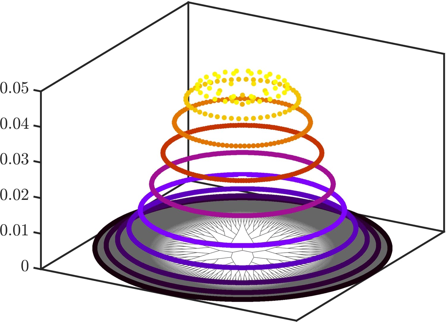
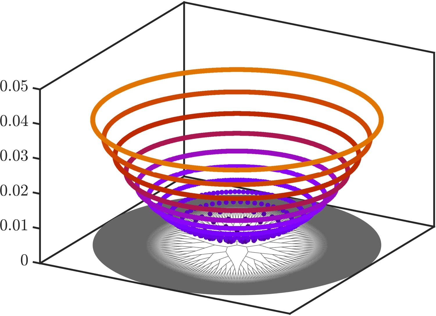
As a consequence, an epidemic can only spread in homogeneous trees of degree $k\geq 2$ when $\mathscr{R}_{0}>1$ and $0<\lambda<\lambda_{c}$. We present in Figure 5 the time evolution of the density of infected individuals $(I_{n}(t))_{n\geq 1}$ solution of system (2.6) from the initial condition depicted in Figure 4 from time $t=0$ to $t=110$ in the case where $\mathscr{R}_{0}>1$ and for $\lambda\in(0,\lambda_{c})$ with $k=2$. We observe the propagation of the infected individuals across the tree.

In that case, we can also characterize at which speed the epidemic spreads into the tree.

We have presented in Figure 6 the spreading speed $c_{*}^{k}$ as a function of the parameter $\lambda$ for several values of $k$, with the convention that when $k=1$, we have $c_{*}^{1}=c_{*}$ where $c_{*}$ is given by Theorem 3. We recover that when $k=1$, that is on the lattice, the spreading speed is a monotone function of $\lambda$. On the other hand, when $k\geq 2$, we observe two key features. First, the spreading speed is no longer monotone. It is strictly increasing up to some critical value $\lambda_{0}>0$ and then strictly decreasing. Second, the spreading speed $c_{*}^{k}$ vanishes at the some critical value of the parameter $\lambda$, and it turns out that this critical value is precisely $\lambda_{c}$ from Theorem 6. We summarize these properties in the following proposition whose proof can be found in [23].

The above result shows that $\lambda_{0}$ maximizes the speed at which the epidemic spreads into the tree. At a given fixed basic reproduction number $\mathscr{R}_{0}>1$, this critical value decreases as $k$ increases, and the associated spreading speed is

$$c_{*}^{k}(\lambda=\lambda_{0})=\frac{\eta(\mathscr{R}_{0}-1)}{\ln k}.$$

This is somehow counterintuitive as one would have expected that the spreading speed would increase with the degree $k$ of the tree.

The remainder of the paper is organized as follows. In Section 3, we present the proofs of our main results regarding the case $\mathcal{G}=\mathbb{Z}$. In the following Section 4, we explain how these proofs transpose to the case of a homogeneous tree $\mathcal{G}=\mathbb{T}_{k}$ for $k\geq 2$. We conclude with a discussion in Section 5.

In section, we study the existence of stationary solutions to (2.2), that is we look for bounded sequences $\left(\mathcal{I}_{j}\right)_{j\in\mathbb{Z}}\in\ell_{\infty}(\mathbb{Z})$ that satisfy

$$0=f(\mathcal{I}_{j})+I_{j}^{0}+\lambda\left(\mathcal{I}_{j-1}-2\mathcal{I}_{j}+\mathcal{I}_{j+1}\right),$$

(3.1)

for each $j\in\mathbb{Z}$. We first remark that the $0$ sequence is a subsolution to the above equation since we assume that $I_{j}^{0}\geq 0$. On the other hand has $f(+\infty)=-\infty$ and each $I_{j}^{0}$ is bounded, there exists some positive real $\rho>0$ such that the constant sequence with $\mathcal{I}_{j}=\rho$ for each $j\in\mathbb{Z}$ is a supersolution of (3.1). We denote by $\left(\overline{\mathcal{I}_{j}}(t)\right)_{j\in\mathbb{Z}}$ the time dependent solution of the Cauchy problem

$$\left\{\begin{split}\mathcal{I}_{j}^{\prime}(t)&=f(\mathcal{I}_{j}(t))+I_{j}^{0}+\lambda\left(\mathcal{I}_{j-1}(t)-2\mathcal{I}_{j}(t)+\mathcal{I}_{j+1}(t)\right),\\ \mathcal{I}_{j}(0)&=\rho,\\ \end{split}\right.$$

(3.2)

for each $j\in\mathbb{Z}$ and $t>0$. Since the constant sequence with $\mathcal{I}_{j}=\rho$ for each $j\in\mathbb{Z}$ is a supersolution of (3.1) it is also a supersolution of (3.2), and it follows from the comparison principle that $\left(\overline{\mathcal{I}_{j}}(t)\right)_{j\in\mathbb{Z}}$ is nonincreasing in the time variable. Furthermore, it satisfies $0\leq\overline{\mathcal{I}_{j}}(t)\leq\rho$ for each $j\in\mathbb{Z}$ and $t>0$. Therefore $\left(\overline{\mathcal{I}_{j}}(t)\right)_{j\in\mathbb{Z}}$ converges as $t\rightarrow+\infty$ to some sequence $\left(\mathcal{I}_{j}^{\infty}\right)_{j\in\mathbb{Z}}$. Thanks to the regularity in time of the solution of the Cauchy problem (3.2), this stationary sequence is solution of (3.1) and by construction $0\leq\mathcal{I}_{j}^{\infty}\leq\rho$ for each $j\in\mathbb{Z}$. As $I_{j}^{0}>0$ for some $j$, we have that the $0$ sequence is not a solution of (3.1). We claim that this implies that $0<\mathcal{I}_{j}^{\infty}$ for each $j\in\mathbb{Z}$. Indeed, assume by contradiction that there exists some $j_{0}\in\mathbb{Z}$ for which $\mathcal{I}_{j_{0}}^{\infty}=0$, the equation (3.1) gives

$$0=I_{j_{0}}^{0}+\lambda\left(\mathcal{I}_{j_{0}-1}^{\infty}+\mathcal{I}_{j_{0}+1}^{\infty}\right).$$

If $j_{0}$ belongs to the support of $\left(I^{0}_{j}\right)_{j\in\mathbb{Z}}$ then we have reached a contradiction. Otherwise, we deduce that $\mathcal{I}_{j_{0}-1}^{\infty}=\mathcal{I}_{j_{0}+1}^{\infty}=0$. We can then repeat the argument such that $j_{0}+k$ belongs to the support of $\left(I^{0}_{j}\right)_{j\in\mathbb{Z}}$ which then leads to a contradiction and proves the claim.

We now derive the limit as $|j|\rightarrow+\infty$. We introduce the sequence of shifts $\mathcal{I}_{j+\tau_{n}}^{\infty}$ with $\tau_{n}\in\mathbb{Z}$ for $n\in\mathbb{N}$ and $|\tau_{n}|\rightarrow+\infty$ as $n\rightarrow+\infty$. Up to subsequences, it converges towards a nonnegative bounded sequence $\left(\widetilde{\mathcal{I}}_{j}\right)_{j\in\mathbb{Z}}$ which satisfies

$$0=f(\widetilde{\mathcal{I}}_{j})+\lambda\left(\widetilde{\mathcal{I}}_{j-1}-2\widetilde{\mathcal{I}}_{j}+\widetilde{\mathcal{I}}_{j+1}\right),\quad j\in\mathbb{Z}.$$

Next, we remark that if $\mathscr{R}_{0}\leq 1$, then $f^{\prime}(0)\leq 0$ and $f<0$ on $(0,+\infty)$ from which we readily deduce that $\widetilde{\mathcal{I}}_{j}=0$ for all $j\in\mathbb{Z}$. This proves that $\underset{|j|\rightarrow+\infty}{\lim}\mathcal{I}_{j}^{\infty}=0$ when $\mathscr{R}_{0}\leq 1$. Now, if $\mathscr{R}_{0}>1$ we note that the sequence $\left(\mathcal{I}_{j}^{\infty}\right)_{j\in\mathbb{Z}}$ is a supersolution to the Fisher-KPP equation set on the lattice $\mathbb{Z}$

$$\mathcal{I}_{j}^{\prime}(t)=f(\mathcal{I}_{j}(t))+\lambda\left(\mathcal{I}_{j-1}(t)-2\mathcal{I}_{j}(t)+\mathcal{I}_{j+1}(t)\right),\quad j\in\mathbb{Z},\quad t>0.$$

For this equation, we know that any solution with a positive, bounded initial condition converges locally uniformly on $\mathbb{Z}$ as $t\rightarrow+\infty$ to the positive zero of $f$ which is denoted $\mathcal{I}_{*}>0$ (see [30, 23]). By comparison, we must have $\mathcal{I}_{j}^{\infty}\geq\mathcal{I}_{*}$ for each $j\in\mathbb{Z}$. This also shows that necessarily $\widetilde{\mathcal{I}}_{j}\geq\mathcal{I}_{*}$ and we infer that $\widetilde{\mathcal{I}}_{j}=\mathcal{I}_{*}$ since $f<0$ on $(\mathcal{I}_{*},+\infty)$. As a consequence, we have proved that $\underset{|j|\rightarrow+\infty}{\lim}\mathcal{I}_{j}^{\infty}=\mathcal{I}_{*}$ when $\mathscr{R}_{0}>1$.

To conclude the proof of Theorem 1, it remains to show that (3.1) has a unique stationary solution. We distinguish between the cases $\mathscr{R}_{0}>1$ and $\mathscr{R}_{0}\leq 1$.

• •

  Case $\mathscr{R}_{0}>1$. Let $\left(\mathcal{I}_{j}^{\infty}\right)_{j\in\mathbb{Z}}$ and $\left(\mathcal{J}_{j}^{\infty}\right)_{j\in\mathbb{Z}}$ be two positive, bounded solutions to (3.1). Since $\mathcal{I}_{j}^{\infty},\mathcal{J}_{j}^{\infty}\geq\mathcal{I}_{*}$ and both $\mathcal{I}_{j}^{\infty}$ and $\mathcal{J}_{j}^{\infty}$ are bounded for each $j$, we have that

  $$\theta:=\underset{j\in\mathbb{Z}}{\sup}~\frac{\mathcal{I}_{j}^{\infty}}{\mathcal{J}_{j}^{\infty}}>0,$$

  is a well-defined quantity. Assume by contradiction that $\theta>1$. Since $\underset{|j|\rightarrow+\infty}{\lim}\mathcal{I}_{j}^{\infty}=\underset{|j|\rightarrow+\infty}{\lim}\mathcal{J}_{j}^{\infty}=\mathcal{I}_{*}$, we have that the above supremum is a maximum attained at some $j_{0}\in\mathbb{Z}$. We obtain by subtracting the equations evaluated at $j=j_{0}$ that

  $$0=f(\mathcal{I}_{j_{0}}^{\infty})-\theta f(\mathcal{J}_{j_{0}}^{\infty})+\underbrace{I_{j_{0}}^{0}(1-\theta)}_{<0}+\underbrace{\lambda\left(\mathcal{I}_{{j_{0}}-1}^{\infty}-2\mathcal{I}_{j_{0}}^{\infty}+\mathcal{I}_{{j_{0}}+1}^{\infty}\right)-\theta\lambda\left(\mathcal{J}_{{j_{0}}-1}^{\infty}-2\mathcal{J}_{j_{0}}^{\infty}+\mathcal{J}_{{j_{0}}+1}^{\infty}\right)}_{\leq 0}.$$

  This yields that

  $$\theta f(\mathcal{J}_{j_{0}}^{\infty})\leq f(\mathcal{I}_{j_{0}}^{\infty})=f(\theta\mathcal{J}_{j_{0}}^{\infty}),$$

  which is impossible by concavity of $f$. As a consequence, we have proved that $\mathcal{I}_{j}^{\infty}\leq\mathcal{J}_{j}^{\infty}$ for each $j\in\mathbb{Z}$. By reversing the role of the two solutions, we reach the conclusion.

• •

  Case $\mathscr{R}_{0}\leq 1$. Let $\left(\mathcal{I}_{j}^{\infty}\right)_{j\in\mathbb{Z}}$ and $\left(\mathcal{J}_{j}^{\infty}\right)_{j\in\mathbb{Z}}$ be two positive, bounded solutions to (3.1). Note that they both tend to $0$ as $|j|\rightarrow+\infty$. Take $\epsilon>0$ and denote $\left(\mathcal{J}_{j}^{\infty,\epsilon}\right)_{j\in\mathbb{Z}}$ the sequence with $\mathcal{J}_{j}^{\infty,\epsilon}=\mathcal{J}_{j}^{\infty}+\epsilon$ which satisfies

  $$f(\mathcal{J}_{j}^{\infty,\epsilon})+I^{0}_{j}+\lambda\left(\mathcal{J}_{j-1}^{\infty,\epsilon}-2\mathcal{J}_{j}^{\infty,\epsilon}+\mathcal{J}_{j+1}^{\infty,\epsilon}\right)<0,\quad j\in\mathbb{Z},$$

  since $f$ is decreasing on $\mathbb{R}_{+}$. Assuming by contradiction that $\mathcal{I}_{j}^{\infty}>\mathcal{J}_{j}^{\infty,\epsilon}$ for some $j$, and subtracting the equation for $\mathcal{I}_{j}^{\infty}$ and the strict inequality for $\mathcal{J}_{j}^{\infty,\epsilon}$, we end up with the inequality

  $$\underbrace{f(\mathcal{I}_{j_{0}}^{\infty})-f(\mathcal{J}_{j_{0}}^{\infty,\epsilon})}_{<0}+\underbrace{\lambda\left(\mathcal{I}_{{j_{0}}-1}^{\infty}-2\mathcal{I}_{j_{0}}^{\infty}+\mathcal{I}_{{j_{0}}+1}^{\infty}\right)-\lambda\left(\mathcal{J}_{{j_{0}}-1}^{\infty,\epsilon}-2\mathcal{J}_{j_{0}}^{\infty,\epsilon}+\mathcal{J}_{{j_{0}}+1}^{\infty,\epsilon}\right)}_{\leq 0}>0$$

  for some $j_{0}\in\mathbb{Z}$ where the maximum is attained. And once again, we have reached a contradiction, thus $\mathcal{I}_{j}^{\infty}\leq\mathcal{J}_{j}^{\infty,\epsilon}$ for all $j\in\mathbb{Z}$ and arbitrary $\epsilon>0$ which gives $\mathcal{I}_{j}^{\infty}\leq\mathcal{J}_{j}^{\infty}$ for all $j\in\mathbb{Z}$ and concludes the proof in that case.

References

- [1] D. G. Aronson. The asymptotic speed of propagation of a simple epidemic. Res. Notes Math., 14, pp. 1-23, 1977.
- [2] F. Ball and T. Britton. Epidemics on networks with preventive rewiring. ArXiv , arXiv:2008.06375, 2020.
- [3] H. Berestycki, J.-M. Roquejoffre and L. Rossi. Propagation of epidemics along lines with fast diffusion. Bull. Math. Biol. 83.1, pp. 1-34, 2021.
- [4] H. Berestycki, S. Nordmann, and L. Rossi. Modeling propagation of epidemics, social unrest and other collective behaviors. arXiv preprint arXiv:2005.09865, 2020.
- [5] C Besse and G Faye. Dynamics of epidemic spreading on connected graphs. Journal of Mathematical Biology 82 (6), pp. 1-52, 2021.
- [6] H. A. Bethe. (1935). Statistical theory of superlattices. Proc. Roy. Soc. Lond. A. 150 (871): 552?575, 1935.
- [7] B. Bollobás. Modern graph theory. Springer Science & Business Media, vol.184, 2013.
- [8] L. Bonnasse-Gahot, H. Berestycki, M.-A. Depuiset, M. B. Gordon, S. Roché, N. Rodriguez, and J.-P. Nadal. Epidemiological modelling of the 2005 French riots: a spreading wave and the role of contagion. Scientific Reports, 8, 2018.
- [9] T. Britton, M. Deijfen, M. Lindholm, and A. Nordvall Lageras. Epidemics on random graphs with tunable clustering. J. Appl. Prob., 45, 743-756, 2008.
- [10] D. Brockmann and D. Helbing. The hidden geometry of complex, network-driven contagion phenomena. Science, 342(6164), pp.1337-1342, 2013.
- [11] R. Burioni, S. Chibbaro, D. Vergni and A. Vulpiani. Reaction spreading on graphs. Physical Review E, 86(5), p.055101, 2012.
- [12] X. Chen. Existence, uniqueness, and asymptotic stability of traveling waves in nonlocal evolution equations. Advances in Differential Equations, 2(1), pp.125-160, 1997.
- [13] X. Chen and J.S. Guo. Existence and Asymptotic Stability of Traveling Waves of Discrete Quasilinear Monostable Equations. Journal of Differential Equations 184, pp. 549-569, 2002.
- [14] X. Chen, S.-C. Fu and J.S Guo. Uniqueness and asymptotics of traveling waves of monostable dynamics on lattices. SIAM J. Math. Anal. vol 38, no 1, pp. 233-258, 2006.
- [15] Y.Y. Chen, J.S. Guo, and F. Hamel. Traveling waves for a lattice dynamical system arising in a diffusive endemic model. Nonlinearity, 30(6), 2334, 2017.
- [16] L.M. Chen, M. Holzer, A. Shapiro. Estimating epidemic arrival times using linear spreading theory. Chaos: An Interdisciplinary Journal of Nonlinear Science, 28(1), p.013105, 2018.
- [17] R.M. Corless, G.H. Gonnet, D.E. Hare, D.J. Jeffrey and D.E. Knuth. On the LambertW function. Advances in Computational mathematics, 5(1), 329-359, 1996.
- [18] O. Diekmann, J.A.P. Heesterbeek, J.A.J. Metz. On the definition and the computation of the basic reproduction ratio in models for infectious diseases in heterogeneous populations. J. Math. Biol., 28, p. 365, 1990.
- [19] A. Ducrot and T. Giletti. Convergence to a pulsating travelling wave for an epidemic reaction-diffusion system with non-diffusive susceptible population. Journal of mathematical biology 69.3, pp. 533-552, 2014.
- [20] S.C. Fu, J.S. Guo, and C-C. Wu. Traveling wave solutions for a discrete diffusive epidemic model. J. Nonlinear Convex Anal, 17, pp.1739-1751, 2016.
- [21] H.W. Hethcote. The mathematics of infectious diseases. SIAM Rev. 42 (4) 599–653, 2000.
- [22] J. Hindes, S. Singh, C.R. Myers and D.J. Schneider. Epidemic fronts in complex networks with metapopulation structure. Physical Review E, 88(1), p.012809, 2013.
- [23] A. Hoffman and M. Holzer. Invasion fronts on graphs: The Fisher-KPP equation on homogeneous trees and Erdös-Réyni graphs. Discrete & Continuous Dynamical Systems-B 24.2: 671, 2019.
- [24] W. O. Kermack, A. G. McKendrick. A contribution to the mathematical theory of epidemics. Proc. Roy. Sot. Ser. A, 115, pp. 700-721, 1927.
- [25] H. Matano, F. Punzo, and A. Tesei. Front propagation for nonlinear diffusion equations on the hyperbolic space. Journal of the European Mathematical Society, 17(5), pp.1199-1227, 2015.
- [26] F.D. Sahneh,C. Scoglio, and P. Van Mieghem. Generalized epidemic mean-field model for spreading processes over multilayer complex networks. IEEE/ACM Transactions on Networking, 21(5), 1609-1620, 2013.
- [27] K. Spricer and T. Britton. An SIR epidemic on a weighted network. Network Science, 7:556-580, 2019.
- [28] L.M. Stolerman, D. Coombs, and S. Boatto. ” SIR-network model and its application to dengue fever. SIAM Journal on Applied Mathematics, 75.6: 2581-2609, 2015.
- [29] P. Van den Driessche and J. Watmough. Reproduction numbers and sub-threshold endemic equilibria for compartmental models of disease transmission. Mathematical biosciences, 180.1-2: 29-48, 2002.
- [30] H. Weinberger. Long-time behavior of a class of biological models. SIAM journal on Mathematical Analysis 13.3, pp. 353-396, 1982.
- [31] C-C. Wu. Existence of traveling waves with the critical speed for a discrete diffusive epidemic model. Journal of Differential Equations 262.1, pp. 272-282, 2017.
- [32] B. Zinner, G. Harris and W. Hudson. Traveling Wavefronts for the Discrete Fisher’s Equation. Journal of Differential Equations 105, pp. 46-62, 1991.