Programmable Interactions and Emergent Geometry in an Atomic Array

We begin by loading rubidium-87 atoms from a magneto-optical trap (MOT) into an array of microtraps, where we use optical pumping and adiabatic microwave sweeps to prepare the atoms in the $\left|{F=1,m=0}\right\rangle$ state. We then transfer the atoms into a 1560 nm optical lattice supported by the cavity, resulting in a set of $M=16$ or 18 discrete ensembles. To generate programmable interactions between the ensembles, we apply a magnetic field gradient and drive the optical cavity along its axis with a modulated intensity. After the interaction time, we load the atoms back into the microtraps and use state-selective fluorescence imaging to measure the population in each Zeeman state. To measure the transverse magnetization, we apply a series of local spin rotations prior to the imaging sequence. Ext. Data Fig. 1a shows a schematic of the experimental sequence.

Our experiments employ a hybrid trapping scheme: whereas we perform cooling, internal state preparation, and imaging in a microtrap array, we transfer the atoms to an intracavity optical lattice before inducing cavity-mediated interactions. The 1560 nm intracavity lattice is in registry with the standing wave of 780 nm light used to drive interactions, and thus maximizes the atom-light coupling. However, because the 1560 nm light produces a strong and inhomogeneous ac Stark shift of the $5P_{3/2}$ state Lee et al. 2014, we instead use the 808 nm microtrap array during portions of the experimental sequence requiring near-resonant light, namely cooling, optical pumping, and fluorescence imaging.

We initially turn on a two-dimensional array of $M\times 2$ optical microtraps at 808 nm during MOT loading. The long axis of the array is aligned with the cavity axis, with $60\,\mu\mathrm{m}$ between traps. The two transverse traps are designed to double the total trap volume and, correspondingly, the number of atoms loaded into the cavity for a fixed microtrap waist. Each microtrap has a waist of $6\,\mu\mathrm{m}$ and a depth of $h\times 4\,\text{MHz}$. During the loading phase the transverse microtrap spacing is $100\,\mu\mathrm{m}$. After loading the microtraps, the transverse spacing is reduced to $8\,\mu\mathrm{m}$, so that both transverse traps fit within the $25\,\mu\mathrm{m}$ waist of the intracavity lattice. We adiabatically transfer the atoms from the microtraps into the intracavity lattice, increasing the lattice power from an initial depth of $h\times 200\,\text{kHz}$ to $h\times 3.5\,\text{MHz}$ and then ramping off the microtraps. This preparation results in 1D array of $M$ ensembles at a temperature of $100\,\mu\mathrm{K}$, with each ensemble containing $n\approx 10^{4}$ atoms spread over 10 lattice sites.

For imaging, we transfer the atoms from the optical lattice back into the microtrap array by first switching on the $M\times 2$ microtraps before reducing the lattice depth to $h\times 200\,$kHz. Subsequently, we adiabatically move the microtraps away from the optical lattice by approximately 15 $\mu$m to avoid ac Stark shifts during imaging.

We detect the atoms in a sequence of four fluorescence images designed to independently measure the populations of all three Zeeman states within the $F=1$ manifold and any residual atoms in $F=2$. For each fluorescence image we apply a retro-reflected laser beam resonant with the $F=2\rightarrow F^{\prime}=3$ transition of the D2 line for 100 $\mu\mathrm{s}$ and collect the resulting fluorescence signal on an EMCCD camera. With the first imaging pulse, we measure the population in the $F=2$ manifold, expelling these atoms from the microtraps by heating. For state-selective imaging of the $F=1$ manifold, we sequentially apply three microwave sweeps which adiabatically transfer the atoms from each magnetic substate to $F=2$ and perform fluorescence imaging after each sweep. A typical fluorescence signal of the atoms is shown in Ext. Data Fig. 1b. For background subtraction we use a method from Xu et al. Xu et al. 2019 based on a principal component analysis of approximately 100 images without atoms.

To measure the transverse spin component $F^{x}_{i}$ we sequentially perform local spin rotations at each site $i$ prior to the imaging sequence. For this purpose, we focus a circularly polarized laser onto each site by controlling the position of the beam with an acousto-optic deflector. By modulating the intensity of the laser at the local Larmor frequency, we induce a resonant Raman coupling between adjacent magnetic sublevels. We apply a $3\,\mu$s Raman pulse to produce a $\pi/2$ spin rotation. This locally maps $F^{x}_{i}$ onto the measurable population difference $n_{+,i}-n_{-,i}$, illustrated in Ext. Data Fig. 1c. Here, $F^{x}_{i}$ is defined in a rotating frame that depends on the local Larmor frequency at site $i$. Shot-to-shot fluctuations in the Larmor frequency lead to a reduction of measurable correlations between two sites, where the reduction depends on the time between the corresponding Raman pulses. Thus, to suppress any bias in the measured correlations, we randomize the order of the local spin rotations in each experimental realization.

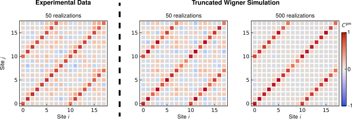
When visualizing the distance-dependence of interactions, reconstructing effective geometries, or probing bipartite correlations, we compute correlation functions $C^{\mathrm{pm}}$, $C^{xx}$, and $C_{b}$ from a minimum of 50 measurements. Each correlation function is defined in the main text in terms of specified observables $A$ and $B$ as

where $\mathrm{Cov}(A,B)\equiv\left\langle AB\right\rangle-\left\langle A\right\rangle\left\langle B\right\rangle$ and $\mathrm{Var}(A)\equiv\mathrm{Cov}(A,A)$. These correlations are normalized to the shot-to-shot variance, which provides the relevant spatial information while being agnostic to the the total amount of pair creation. Effects of finite statistics on the measured correlations $C^{\mathrm{pm}}$ are examined in Ext. Data Fig. 2.

To quantify pair creation dynamics, we measure in the $\hat{x}$-basis and normalize the covariance matrices to the population of atoms on each site rather than their variance,

For this correlator, the measurement in the $\hat{x}$-basis provides a high sensitivity at early times and a large dynamic range for measurements over time. The normalization is chosen such that the extracted correlation is sensitive to the total amount of pair creation, allowing us to visualize the growth of correlations as a function of time.

To enable the programmable interactions, we apply a magnetic field gradient parameterized by the difference $\omega_{B}$ in Zeeman splittings between adjacent array sites. This gradient is superposed on an overall bias field $B_{0}$ perpendicular to the cavity axis, which produces a Zeeman splitting of $\omega_{z}/B_{0}=2\pi\times 700\,\text{kHz}/\text{G}$ and a quadratic Zeeman shift of $q/B_{0}^{2}=2\pi\times 72\,\text{Hz}/\text{G}^{2}$. We work in a regime where $\omega_{z}/M>\omega_{B}>q$, i.e., the variation in the magnetic field is small compared to the average field yet results in a Bloch oscillation frequency larger than the quadratic Zeeman shift. Specifically, we choose a magnetic field between 2 and 4 G (as detailed in Ext. Data Table 1 for each data set) and a typical gradient $\omega_{B}=2\pi\times 1.52(1)\,\text{kHz/site}$. For measurements of $C^{\text{pm}}$ in Figs. 1-2, we increase the ratio $\omega_{B}/q$. This is accomplished either by increasing $\omega_{B}$ to $2\pi\times 12.47(2)\,\text{kHz}$, or by reducing the effective quadratic Zeeman shift to $q=2\pi\times 60\,\text{Hz}$ by applying an ac Stark shift to the $\left|{1,0}\right\rangle$ state via off-resonant microwave coupling to $\left|{2,0}\right\rangle$.

We induce spin-exchange interactions among the atoms by applying a drive field which typically has a detuning between $\delta_{c}=-2\pi\times 4\,\text{MHz}$ and $-2\pi\times 7\,$MHz from cavity resonance. The cavity mode itself has a large detuning of $\Delta=-2\pi\times 11\,$GHz from atomic resonance. The drive field is linearly polarized at an angle of 55 degrees with respect to the magnetic field, chosen to eliminate tensor light shifts. The instantaneous spin-exchange coupling is given by $-\tilde{J}\approx\bar{n}_{\text{ph}}\Omega^{2}/(2\delta_{c})$, where $\Omega=2\pi\times 13\,\text{Hz}$ is the vector ac Stark shift per circularly polarized photon in the cavity. Our typical peak intracavity photon number $\bar{n}_{\text{ph}}=10^{4}$ corresponds to a collective interaction strength $2n\tilde{J}=2\pi\times 3\,\text{kHz}$ between ensembles of $n=10^{4}$ atoms.

To produce a set of couplings $J(r)$, we modulate the intensity of the drive field via an acousto-optic modulator as

where we use the phases $\phi_{r}\in\{0,\pi\}$ to set the sign of the interactions. The coupling at $r=0$ is given by $J(0)=2\sum_{r>0}|J(r)|$. To produce periodic boundary conditions in the system of $M$ sites, we additionally pulse the drive at a frequency of $M\omega_{B}$. Each pulse has a duration of $0.3\tau_{B}/M=11\mu\mathrm{s}$.

The atoms are coupled to a near-concentric Fabry-Perot cavity with a length of 5  cm and an $18\,\mu\mathrm{m}$ waist at 780 nm. The cavity has vacuum Rabi frequency of $2g=2\pi\times 2.6\,\text{MHz}$ and linewidth $\kappa=2\pi\times 250(20)\,\text{kHz}$, yielding a single-atom cooperativity $\eta=\frac{4g^{2}}{\kappa\Gamma}=4.5$, where $\Gamma=2\pi\times 6.07\,\text{MHz}$ is the linewidth of the $5P_{3/2}$ state in rubidium. Our drive field is detuned by $\Delta=-2\pi\times 11\,\text{GHz}$ from the $\left|{5S_{1/2},F=1}\right\rangle\rightarrow\left|{5P_{3/2}}\right\rangle$ transition, which produces a vector light shift per circularly polarized photon of $\Omega_{0}=-\frac{g^{2}}{6\Delta}=2\pi\times 26\,\text{Hz}$ on a maximally coupled atom at cavity center. For an average atom this dispersive coupling is reduced to $\Omega=2\pi\times 13\,\text{Hz}$, primarily by thermal motion. The Rayleigh range of the cavity is $z_{R}=1.3\,\text{mm}$, and each ensemble is within $0.4z_{R}=520\,\mu\mathrm{m}$ of cavity center. Displacement from cavity center contributes up to a 20% reduction in coupling for the most distant atoms.

In Eq. (1), we describe the distance-dependent spin-exchange interactions by a static effective Hamiltonian $H_{I}$, with the spin on each site defined in a rotating frame set by the local magnetic field. Here we summarize the derivation of the effective Hamiltonian starting from the full time-dependent Hamiltonian $H_{\mathrm{lab}}$ in the lab frame. The Hamiltonian $H_{\mathrm{lab}}$ for the spin system, obtained by adiabatically eliminating the cavity mode Davis et al. 2019; Davis et al. 2020, is given by

in terms of the collective spin $\mathbf{F}_{l}=\sum_{\mu\in l}\mathbf{f}_{\mu}$ on each site $l$, the local magnetic fields $h_{l}=\omega_{B}l$, and the quadratic Zeeman shift $H_{q}=q\sum_{\mu}(f^{z}_{\mu})^{2}$, in units where $\hbar=1$. Moving to a rotating frame with $H_{0}=\sum_{l}h_{l}F^{z}_{l}$, the Hamiltonian becomes

When the collective interaction strength and quadratic Zeeman shift are weak compared to the gradient ($nJ,q\ll\omega_{B}$), the effective Hamiltonian is given to first order by the time average of Eq. (8). The interaction component of the resulting effective Hamiltonian $H_{I}+H_{q}$ is

where

The dependence $J(r)$ of the couplings on distance is thus given by the Fourier transform of the drive waveform.

To analytically compute the dynamics of the system, we write the Hamiltonian without approximation in terms of spin-wave operators $\tilde{F}^{+}_{k=\omega_{B}t}\equiv\frac{1}{\sqrt{M}}\sum_{l}e^{-ikl}{F}^{+}_{l}$, as

We can understand this Hamiltonian by recognizing that, in the lab frame, the magnetic field gradient causes spin waves to undergo Bloch oscillations at frequency $\omega_{B}$. Only spin waves with momentum $k=0$ in the lab frame couple to the cavity. In the rotating frame set by the gradient, the same physics can be viewed as spin waves remaining static over time while the mode to which the cavity couples is given by $k=\omega t$. The quadratic Zeeman shift is left unchanged by the change of reference frames.

Since the system is finite and discrete, there are only $M$ orthogonal momentum modes. To obtain a discrete set of momentum-space couplings $\tilde{J}_{k}=-\chi_{k}/2n$, we drive interactions with a pulsed drive $\tilde{J}(t)=\sum_{k}\frac{2\pi}{M}\tilde{J}_{k}\delta(\omega_{B}t-k)$ that only takes on non-zero values $M$ times per Bloch period. We observe that the momentum modes decouple in the Hamiltonian,

The evolution of any given momentum mode is discrete, with a short period of coupling to the optical cavity that induces spin-spin interactions, followed by a longer period of time when the state evolves only under the quadratic Zeeman shift. In the limit of a large collective interaction strength $|\chi_{k}|>\omega_{B}$, each momentum mode grows by a factor of $\lambda\approx|2\chi_{k}\tau_{B}|\sin(q\tau_{B})$ after each Bloch period (see Supplementary Information). This growth is reflected by the structure factor, with ${|\tilde{F}^{x}_{k}|\propto|\chi_{k}|^{T}\propto|\tilde{J}(k/\omega_{B})|^{T}}$ after $T$ Bloch periods.

While our derivation of the growth of the structure factor assumes a pulsed drive field, which produces periodic boundary conditions, the same relation provides a good approximation in the case of a continuous drive field that produces open boundary conditions. In the latter case, we expect small deviations from the model because the cavity couples to a continuum of non-orthogonal momentum modes. We compare the continuous and pulsed cases in a numerical simulation presented in Ext. Data Fig. 3.

A key feature of the evolution in momentum space is that the modes with minimum energy are maximally amplified in our system with $\chi_{k}<0$. We can gain additional intuition for this effect by considering the limit where the dynamics are slow compared to the Bloch period and a time-averaged Hamiltonian is valid. In this case, the dynamics for each momentum mode are identical to the single-mode case that has been studied previously Davis et al. 2019; Stamper-Kurn and Ueda 2013. The system is unstable to pair creation when the collective interaction strength $2\chi_{k}=-4n\tilde{J}_{k}$ has a greater magnitude and opposite sign from the quadratic Zeeman shift $q$. This condition motivates our choice of ferromagnetic on-site interactions, such that ${\chi_{k}<0}$, in our system with $q>0$. The opposite signs of $\chi$ and $q$ allow the system to access low-energy states of the interaction Hamiltonian $H_{I}$ by transferring energy into $H_{q}$ via pair creation.

We leverage our understanding of the pair-creation dynamics to reconstruct effective coordinates $\boldsymbol{\rho}$ and inferred couplings $J^{\prime}$ directly from measured correlations $C^{xx}$. Specifically, building on our analytical model for the growth of the structure factor, we here derive the Gaussian ansatz for the decay of correlations with distance in the effective geometry. The dynamical evolution produces low energy states of the XY Hamiltonian, which additionally allows us to relate the inverse correlation matrix and the inferred couplings.

To analytically motivate the Gaussian ansatz used for reconstructing effective geometries, we begin by relating the structure factor to the correlations we measure in the $\hat{x}$-basis,

The final equality holds when the momentum modes are independent from one another, such that cross terms with $k_{1}\neq k_{2}$ go to zero. This is true either when periodic boundary conditions are imposed or in the limit of an infinite system. Equation (13) allows for predicting the form of spatial correlations from the dispersion relation $\chi_{k}$, which governs the growth of the structure factor.

As an illustrative example, we consider nearest-neighbor interactions created by the drive waveform $\tilde{J}(t)\propto(\cos\omega_{B}t+1)$, corresponding to the dispersion relation

Since the correlations are the Fourier transform of the squared magnitude of the structure factor, we write an expansion of $|\tilde{F}^{x}_{k}|^{2}$ in terms of powers of $e^{ik}$. Recalling $|\tilde{F}^{x}_{k}|\propto|\chi_{k}|^{T}$ after $T$ Bloch periods of evolution, we compute

The coefficients in this expansion are Fourier components corresponding to correlations at distance $d$. Thus, we have $C^{xx}(d)\propto{{4T}\choose{d+2T}}$. This binomial coefficient tends to a Gaussian function of distance $d$ after several Bloch periods, analogously to a diffusion process.

More generally a multi-frequency drive leads to diffusion within the effective geometry set by the couplings. For a generic drive that produces a dispersion relation $\chi_{k}\propto-\sum_{r}J(r)e^{ikr}$, correlations in position space are given by terms in the multinomial expansion of $|\chi_{k}|^{2T}$. When $J(r)>0$ this directly corresponds to a random walk within the effective geometry set by the couplings $J(r)$. Motivated by the exact result for spreading in 1D, we use a Gaussian ansatz for the correlation matrix to infer distances and hence the coordinates $\boldsymbol{\rho}$ within the effective geometry.

We motivate the inferred coupling matrix $J^{\prime}=\left(C^{xx}\right)^{-1}$ by recalling that a population growth rate given by $|\chi_{k}|$ generates a low energy state of the XY model, $H_{I}$. We approximate the final state as thermal, with large inverse temperature $\beta$. We make use of the $SO(2)$ symmetry to note that $\left\langle F^{x}_{i}F^{x}_{j}\right\rangle$ and $\left\langle F^{y}_{i}F^{y}_{j}\right\rangle$ are equivalent. Now, to compute $\left\langle F^{x}_{i}F^{x}_{j}\right\rangle$, we integrate over phase space, with a Boltzmann weighting $\exp(-\beta H_{I})$. To constrain the overall spin length, we introduce a chemical potential $\mu$, so that

The chemical potential can be incorporated into a modified coupling matrix ${J_{ij}^{\prime}=J_{ij}-\mu\delta_{ij}}$. Evaluating the integral yields $C^{xx}\propto J_{ij}^{\prime-1}$. For the purposes of the reconstruction in Fig. 3, where we color bonds between sites according to $J_{ij}^{\prime}$, only the off-diagonal terms of $J_{ij}^{\prime}$ are relevant.

The inverse correlation matrix, also known as the concentration or precision matrix, can also be interpreted as the partial correlation matrix Lauritzen 1996, up to normalization. For a given set of variables $x_{i}$, the partial correlation between $x_{i}$ and $x_{j}$ is the correlation after regressing out every $x_{l\neq i,j}$. In a system with interactions at distance $r$, sites spaced by $r$ have a non-zero partial correlation, but sites at distances that are multiples of $r$ have zero partial correlation, since the interactions between the sites at distance $r$ mediate all the variance. Thus, the interpretation of the inverse correlation matrix as an inferred coupling matrix ${J^{\prime}\propto\left(C^{xx}\right)^{-1}}$ is well motivated even at early times, when correlations are still spreading across the system.

In the absence of a magnetic field gradient, the optical cavity in our system mediates interactions between all pairs of atoms, irrespective of the distance between them Davis et al. 2019; Davis et al. 2020. For a magnetic field oriented perpendicular to the cavity axis, interactions are well described by an all-to-all spin-exchange Hamiltonian. We approximate all spins as uniformly coupled to the cavity and parameterize the atom-light interaction by the vector light shift $\Omega$ produced by a circularly polarized intracavity photon. In this limit, the interaction Hamiltonian and spin exchange couplings are

where $\boldsymbol{F}=\sum_{\mu}{\mathbf{f}_{\mu}}$ is the collective spin for all atoms, $\kappa$ is the cavity linewidth, and $\bar{n}_{\text{ph}}(t)$ is the instantaneous intracavity photon number. The strength and sign of interaction depend on the detunings $\delta_{\pm}=\delta_{c}\mp\omega_{z}$ from two-photon resonances that flip a single spin, given in terms of the detuning $\delta_{c}$ of the drive field from cavity resonance and Zeeman splitting $\omega_{z}$ Davis et al. 2019; Davis et al. 2020.

The interaction Hamiltonian can be rewritten in terms of a single interaction strength $\tilde{J}(t)=-(\tilde{J}_{+}+\tilde{J}_{-})$ as

where we have defined $\tilde{J}$ to be positive for ferromagnetic interactions. The final term in Eq. (S4) acts as a uniform field along $\hat{z}$ and is suppressed by a factor of $n$ as compared to the collectively enhanced interactions between ensembles of $n$ atoms. This term can always be ignored by operating in a suitable rotating frame, and in our case its value of $2\tilde{J}_{-}=2\pi\times 0.2\,\text{Hz}$ is negligibly small because it is not collectively enhanced.

To obtain a localized effective Hamiltonian that supports pair creation dynamics, we include the terms for a magnetic field gradient proportional to $\omega_{B}$ and quadratic Zeeman shift $q$. The full time-dependent Hamiltonian for our array of atomic ensembles is then

where $\mathbf{F}_{l}=\sum_{r_{\mu}=l}\mathbf{f}_{\mu}$ represents the collective spin on each site $l$. Viewing each site in a frame rotating at the local Larmor frequency $l\omega_{B}$, we can recast the Hamiltonian as

For sufficiently weak couplings that are modulated periodically at harmonics of the Bloch frequency $\omega_{B}$, with $n\tilde{J}(t),q<\omega_{B}$, the Floquet Hamiltonian for the system is well approximated by the time-averaged Hamiltonian, which is the lowest order term of the Floquet-Magnus expansion Bukov et al. 2015,

Here we have defined $J(r)=J(l-m)$ using the Fourier transform of $\tilde{J}(t)$ evaluated at frequency $r\omega_{B}$,

We can realize arbitrary couplings $J(r)$, subject to the hermiticity condition $J(r)=J^{*}(-r)$, by using the drive waveform

Since our scheme generates translationally invariant interactions, it is natural to write the Hamiltonian in momentum space, in terms of spin-wave operators

The translation invariance is exact in the limit of a large system ($M\rightarrow\infty$) or for a drive chosen to induce periodic boundary conditions, $J(r)=J(M-r)$. For these cases, we can rewrite Eq. (S7) in terms of spin-wave operators to obtain the momentum-space representation of the Hamiltonian

with momentum-space couplings given by

where $\delta_{M}(x)\equiv(1-e^{iMx})/({1-e^{ix}})$ tends to a Dirac delta function in the limit of an infinite system.

We initialize the system with all atoms in $m=0$, and for early times we can approximate the atoms in this state as a constant classical pump field that drives the formation of correlated atom pairs in states $m=\pm 1$ Davis et al. 2019. In this regime, the Hamiltonian can be expressed in terms of bosonic operators $a^{\dagger}_{i}$ ($b^{\dagger}_{i}$) representing the creation of an atom in state $m=1$ ($m=-1$) on site $i$ (see Eq. S17 below) or, alternatively, the momentum-space counterparts $a^{\dagger}_{k},b^{\dagger}_{k}$. In terms of these bosonic operators, the spin-wave operators can be written as

and the interaction Hamiltonian is

This shows that $\chi_{k}=-2n\tilde{J}_{k}$ is the dispersion relation for spin excitations. This is identical to the dispersion relation obtained from a Holstein-Primakoff transformation in the vicinity of a spin-polarized state.

In this section we present an analytical derivation of the dynamics of our system at early times, when we can neglect depletion of atoms in $m=0$. In contrast to the previous sections, the derivations here do not require the limit of weak interactions and capture the discretized nature of the dynamics over each Bloch period. Our approach will be to express the full time-dependent Hamiltonian in terms of spin-wave operators. Solving for the dynamics of the spin waves facilitates the computation of the structure factor and spatial correlations. We start with the Hamiltonian in the rotating frame as written in Eq. (S6). We recognize that the interaction term can be written succinctly in terms of spin-wave operators $\tilde{\mathbf{F}}_{k}$. The full expression for this Hamiltonian is

where $H_{q}=q\sum_{\mu}(f^{z}_{\mu})^{2}$ is the quadratic Zeeman shift. Since the system is finite, there are only $M$ orthogonal momentum modes, whereas the cavity couples to a continuous range of momenta $k=\omega_{B}t$ during a single Bloch period. Generically this couples adjacent momentum modes. In the limit of an infinite system, the modes become fully independent.

The modes are also fully independent in the case where we generate periodic boundary conditions using a pulsed drive field. In this case, the instantaneous spin-exchange coupling $\tilde{J}(t)=\sum_{k}\frac{2\pi}{M}\tilde{J}_{k}\delta(\omega_{B}t-k)$ only takes on non-zero values $M$ times per Bloch period, and we observe that the momentum modes decouple in the Hamiltonian

For any given momentum mode, the evolution is discrete, with a short period of coupling to the optical cavity followed by a longer period of time when the state is acted upon by the quadratic Zeeman shift. In the limit of weak interactions and many Bloch periods, this trotterized Hamiltonian becomes identical to $M$ independent continuous pair-creation processes in different momentum modes.

In order to analytically solve for the dynamics of pair creation, we define three bosonic modes on each site $a_{i}$, $b_{i}$, $c_{i}$ corresponding to atoms on site $i$ in the states $m=\pm 1,0$ respectively. For early times we can treat the atom initialized in $m=0$ as a classical pump field with $c_{i}=\sqrt{n}$. In this limit we can express the local spin operators as a function of operators for the bosonic modes,

and similarly express the quadratic Zeeman shift as

Following the same convention as for the spin-wave operator $\tilde{F}_{k}$, we define operators for the momentum modes $a_{k}\equiv\frac{1}{\sqrt{M}}\sum_{l}e^{-ikl}a_{l}$ and $b_{k}\equiv\frac{1}{\sqrt{M}}\sum_{l}e^{-ikl}b_{l}$. We can rewrite the key operators in the rotating-frame Hamiltonian (Eq. (S16)) in terms of these bosonic modes,

With the Hamiltonian expressed in terms of the bosonic operators, we can proceed to solve for the dynamics of the system. In particular, we realize that there are independent equations of motion for every discrete value of $k=2\pi m/M$ where $m$ is an integer. In particular, the Heisenberg equations of motion for $a_{k}$ and $b_{-k}^{\dagger}$ depend only on each other,

where $\chi_{k}=-2n\tilde{J}_{k}$ is the dispersion relation. To solve these equations, we write the two operators as a vector $\mathcal{O}=(a_{k},b_{-k}^{\dagger})$. This leads to a matrix equation $\dot{\mathcal{O}}=D(t)\mathcal{O}$ where,

References

- Bloch et al. (2012) I. Bloch, J. Dalibard, and S. Nascimbene, Nat. Phys. 8, 267 (2012).
- Browaeys and Lahaye (2020) A. Browaeys and T. Lahaye, Nat. Phys. 16, 132 (2020).
- Das and Chakrabarti (2008) A. Das and B. K. Chakrabarti, Rev. Mod. Phys. 80, 1061 (2008).
- Gopalakrishnan et al. (2011) S. Gopalakrishnan, B. L. Lev, and P. M. Goldbart, Phys. Rev. Lett. 107, 277201 (2011).
- Strack and Sachdev (2011) P. Strack and S. Sachdev, Phys. Rev. Lett. 107, 277202 (2011).
- McMahon et al. (2016) P. L. McMahon, A. Marandi, Y. Haribara, R. Hamerly, C. Langrock, S. Tamate, T. Inagaki, H. Takesue, S. Utsunomiya, K. Aihara, et al., Science 354, 614 (2016).
- Berloff et al. (2017) N. G. Berloff, M. Silva, K. Kalinin, A. Askitopoulos, J. D. Töpfer, P. Cilibrizzi, W. Langbein, and P. G. Lagoudakis, Nat. Mater. 16, 1120 (2017).
- Hayden and Preskill (2007) P. Hayden and J. Preskill, J. High Energy Phys. 2007, 120 (2007).
- Maldacena and Stanford (2016) J. Maldacena and D. Stanford, Phys. Rev. D 94, 106002 (2016).
- Bentsen et al. (2019) G. Bentsen, T. Hashizume, A. S. Buyskikh, E. J. Davis, A. J. Daley, S. S. Gubser, and M. Schleier-Smith, Phys. Rev. Lett. 123, 130601 (2019).
- Belyansky et al. (2020) R. Belyansky, P. Bienias, Y. A. Kharkov, A. V. Gorshkov, and B. Swingle, Phys. Rev. Lett. 125, 130601 (2020).
- Leroux et al. (2010) I. D. Leroux, M. H. Schleier-Smith, and V. Vuletić, Phys. Rev. Lett. 104, 073602 (2010).
- Barontini et al. (2015) G. Barontini, L. Hohmann, F. Haas, J. Estève, and J. Reichel, Science 349, 1317 (2015).
- Hosten et al. (2016) O. Hosten, N. J. Engelsen, R. Krishnakumar, and M. A. Kasevich, Nature 529, 505 (2016).
- Welte et al. (2018) S. Welte, B. Hacker, S. Daiss, S. Ritter, and G. Rempe, Phys. Rev. X 8, 011018 (2018).
- Pedrozo-Peñafiel et al. (2020) E. Pedrozo-Peñafiel, S. Colombo, C. Shu, A. F. Adiyatullin, Z. Li, E. Mendez, B. Braverman, A. Kawasaki, D. Akamatsu, Y. Xiao, et al., Nature 588, 414 (2020).
- Davis et al. (2019) E. J. Davis, G. Bentsen, L. Homeier, T. Li, and M. H. Schleier-Smith, Phys. Rev. Lett. 122, 010405 (2019).
- Davis et al. (2020) E. J. Davis, A. Periwal, E. S. Cooper, G. Bentsen, S. J. Evered, K. Van Kirk, and M. H. Schleier-Smith, Phys. Rev. Lett. 125, 060402 (2020).
- Muniz et al. (2020) J. A. Muniz, D. Barberena, R. J. Lewis-Swan, D. J. Young, J. R. Cline, A. M. Rey, and J. K. Thompson, Nature 580, 602 (2020).
- Barbón and Magán (2013) J. L. Barbón and J. M. Magán, J. High Energy Phys. 2013, 163 (2013).
- Gubser et al. (2017) S. S. Gubser, J. Knaute, S. Parikh, A. Samberg, and P. Witaszczyk, Commun. Math. Phys. 352, 1019 (2017).
- Heydeman et al. (2016) M. Heydeman, M. Marcolli, I. Saberi, and B. Stoica, arXiv:1605.07639 (2016).
- Qi (2018) X.-L. Qi, Nat. Phys. 14, 984 (2018).
- Rudner and Lindner (2020) M. S. Rudner and N. H. Lindner, Nat. Rev. Phys. 2, 229 (2020).
- Kennedy et al. (2015) C. J. Kennedy, W. C. Burton, W. C. Chung, and W. Ketterle, Nat. Phys. 11, 859 (2015).
- Aidelsburger et al. (2015) M. Aidelsburger, M. Lohse, C. Schweizer, M. Atala, J. T. Barreiro, S. Nascimbène, N. Cooper, I. Bloch, and N. Goldman, Nat. Phys. 11, 162 (2015).
- Struck et al. (2013) J. Struck, M. Weinberg, C. Ölschläger, P. Windpassinger, J. Simonet, K. Sengstock, R. Höppner, P. Hauke, A. Eckardt, M. Lewenstein, et al., Nature Physics 9, 738 (2013).
- Vaidya et al. (2018) V. D. Vaidya, Y. Guo, R. M. Kroeze, K. E. Ballantine, A. J. Kollár, J. Keeling, and B. L. Lev, Phys. Rev. X 8, 011002 (2018).
- Islam et al. (2013) R. Islam, C. Senko, W. C. Campbell, S. Korenblit, J. Smith, A. Lee, E. E. Edwards, C.-C. J. Wang, J. K. Freericks, and C. Monroe, Science 340, 583 (2013).
- Jurcevic et al. (2014) P. Jurcevic, B. P. Lanyon, P. Hauke, C. Hempel, P. Zoller, R. Blatt, and C. F. Roos, Nature 511, 202 (2014).
- Fausti et al. (2011) D. Fausti, R. I. Tobey, N. Dean, S. Kaiser, A. Dienst, M. C. Hoffmann, S. Pyon, T. Takayama, H. Takagi, and A. Cavalleri, Science 331, 189 (2011).
- Wang et al. (2013) Y. H. Wang, H. Steinberg, P. Jarillo-Herrero, and N. Gedik, Science 342, 453 (2013).
- Bohnet et al. (2016) J. G. Bohnet, B. C. Sawyer, J. W. Britton, M. L. Wall, A. M. Rey, M. Foss-Feig, and J. J. Bollinger, Science 352, 1297 (2016).
- Léonard et al. (2017) J. Léonard, A. Morales, P. Zupancic, T. Esslinger, and T. Donner, Nature 543, 87 (2017).
- Hung et al. (2016) C.-L. Hung, A. González-Tudela, J. I. Cirac, and H. J. Kimble, Proc. Natl. Acad. Sci. U.S.A. 113, E4946 (2016).
- Manovitz et al. (2020) T. Manovitz, Y. Shapira, N. Akerman, A. Stern, and R. Ozeri, PRX Quantum 1, 020303 (2020).
- Marsh et al. (2021) B. P. Marsh, Y. Guo, R. M. Kroeze, S. Gopalakrishnan, S. Ganguli, J. Keeling, and B. L. Lev, Phys. Rev. X 11, 021048 (2021).
- Anikeeva et al. (2021) G. Anikeeva, O. Marković, V. Borish, J. A. Hines, S. V. Rajagopal, E. S. Cooper, A. Periwal, A. Safavi-Naeini, E. J. Davis, and M. Schleier-Smith, PRX Quantum 2, 020319 (2021).
- Kollár et al. (2019) A. J. Kollár, M. Fitzpatrick, and A. A. Houck, Nature 571, 45 (2019).
- Masson et al. (2017) S. J. Masson, M. Barrett, and S. Parkins, Phys. Rev. Lett. 119, 213601 (2017).
- Hamley et al. (2012) C. D. Hamley, C. Gerving, T. Hoang, E. Bookjans, and M. S. Chapman, Nat. Phys. 8, 305 (2012).
- Torgerson (1952) W. S. Torgerson, Psychometrika 17, 401 (1952).
- Lee and Lee (1998) S. Lee and K.-C. Lee, Phys. Rev. B 57, 8472 (1998).
- Gubser et al. (2018) S. S. Gubser, C. Jepsen, Z. Ji, and B. Trundy, Phys. Rev. D 98, 045009 (2018).
- Shi et al. (2006) Y.-Y. Shi, L.-M. Duan, and G. Vidal, Phys. Rev. A 74, 022320 (2006).
- Murg et al. (2010) V. Murg, F. Verstraete, Ö. Legeza, and R. M. Noack, Phys. Rev. B 82, 205105 (2010).
- Sekino and Susskind (2008) Y. Sekino and L. Susskind, J. High Energy Phys. 2008, 065 (2008).
- Pastawski et al. (2015) F. Pastawski, B. Yoshida, D. Harlow, and J. Preskill, J. High Energ. Phys. 2015, 149 (2015).
- Amit et al. (1985) D. J. Amit, H. Gutfreund, and H. Sompolinsky, Phys. Rev. A 32, 1007 (1985).
- Pezzè et al. (2018) L. Pezzè, A. Smerzi, M. K. Oberthaler, R. Schmied, and P. Treutlein, Rev. Mod. Phys. 90, 035005 (2018).
- Evans et al. (2018) R. E. Evans, M. K. Bhaskar, D. D. Sukachev, C. T. Nguyen, A. Sipahigil, M. J. Burek, B. Machielse, G. H. Zhang, A. S. Zibrov, E. Bielejec, et al., Science 362, 662 (2018).
- Lee et al. (2014) J. Lee, G. Vrijsen, I. Teper, O. Hosten, and M. A. Kasevich, Opt. Lett. 39, 4005 (2014).
- Xu et al. (2019) V. Xu, M. Jaffe, C. D. Panda, S. L. Kristensen, L. W. Clark, and H. Müller, Science 366, 745 (2019).
- Stamper-Kurn and Ueda (2013) D. M. Stamper-Kurn and M. Ueda, Reviews of Modern Physics 85, 1191 (2013).
- Lauritzen (1996) S. L. Lauritzen, Graphical models, Vol. 17 (Clarendon Press, 1996).
Extended Data
- Bukov et al. (2015) M. Bukov, L. D’Alessio, and A. Polkovnikov, Adv. Phys. 64, 139 (2015).
- Gower (2014) J. C. Gower, Wiley StatsRef: Statistics Reference Online (2014), 10.1002/9781118445112.stat02470.
- Ryu and Takayanagi (2006) S. Ryu and T. Takayanagi, Phys. Rev. Lett. 96, 181602 (2006).
- Hartnoll et al. (2018) S. A. Hartnoll, A. Lucas, and S. Sachdev, Holographic quantum matter (MIT press, 2018).
- Sinatra et al. (2002) A. Sinatra, C. Lobo, and Y. Castin, J. Phys. B: At., Mol. Opt. Phys. 35, 3599 (2002).
- Blakie et al. (2008) P. B. Blakie, A. S. Bradley, M. J. Davis, R. J. Ballagh, and C. W. Gardiner, Adv. Phys. 57, 363 (2008).
- Lewis-Swan et al. (2016) R. J. Lewis-Swan, M. K. Olsen, and K. V. Kheruntsyan, Phys. Rev. A 94, 033814 (2016).