QMUL-PH-21-29
Superstring loop amplitudes from the field theory limit
Abstract
We propose a procedure to determine the moduli-space integrands of loop-level superstring amplitudes for massless external states in terms of the field theory limit. We focus on the type II superstring. The procedure is to: (i) take a supergravity loop integrand written in a BCJ double-copy representation, (ii) use the loop-level scattering equations to translate that integrand into the ambitwistor string moduli-space integrand, localised on the nodal Riemann sphere, and (iii) uplift that formula to one on the higher-genus surface valid for the superstring, guided by modular invariance. We show how this works for the four-point amplitude at two loops, where we reproduce the known answer, and at three loops, where we present a conjecture that is consistent with a previous proposal for the chiral measure. Useful supergravity results are currently known up to five loops.
I Introduction
The birth of string theory is widely considered to be the discovery by Veneziano of the scattering amplitude formula that today bears his name Veneziano 1968. More than five decades later, the calculation of string scattering amplitudes remains a formidable challenge. To give the example of the type II superstring in Minkowski spacetime, the four-point amplitude for massless external states was computed at tree level and one loop in 1982 Green and Schwarz 1982; Schwarz 1982, and at two loops in 2005 D’Hoker and Phong 2005a; Berkovits 2006; Berkovits and Mafra 2006. There has been significant work on the three-loop problem, namely a proposal for the chiral measure D’Hoker and Phong 2005b; D’Hoker and Phong 2005c; Cacciatori et al. 2008a and a partial computation using the pure spinor formalism Gomez and Mafra 2013, but it remains to be fully addressed. The advances have had a rich interplay with those in gauge theory and gravity amplitudes, particularly in their maximally supersymmetric versions. For instance, the first computations of the four-point one-loop amplitudes in the now widely studied 4D super-Yang-Mills theory (SYM) and supergravity were based on the field theory limit of the analogous superstring calculations Green et al. 1982. In this paper, we aim to return the favour by importing three-loop results in supergravity, themselves obtained from non-planar SYM via the Bern-Carrasco-Johansson (BCJ) double copy Bern et al. 2010, into the type II superstring.
II String theory versus field theory
We will consider the type II superstring four-point amplitude for massless incoming states of momenta . The 10D maximal supersymmetry implies that information on the four external states is encoded in a kinematic prefactor Green et al. 1988, such that the supergravity tree-level amplitude is . We define the Mandelstam variables as . Our working assumption will be that, up to three loops 11 1 Beyond three loops, the integration over the period matrix must be restricted due to the Schottky problem. Beyond four loops, the delicate issue of non-projectedness of supermoduli space is also known to arise Donagi and Witten 2015., the -loop superstring amplitude takes the form
| (1) |
The integration denoted by is over a genus- fundamental domain parametrised by the period matrix () and over four marked points . We use a ‘chiral splitting’ representation D’Hoker and Phong 1988; D’Hoker and Phong 1989, made possible by the introduction of the loop momenta , with denoting . The appearance of the prime form and the exponential (involving the holomorphic Abelian differentials whose cycles define the period matrix) constitute the chiralanti-chiral loop-level Koba-Nielsen factors. The interesting object is . We make no distinction between type IIA and type IIB apart from the details of , since at four points there is no contribution from odd spin structures at least up to three loops 22 2 This follows from supersymmetry and is clear if we consider factorisable NS-NS external states . The supersymmetric pre-factor is , where is the pre-factor for the open superstring and includes products . At three loops and four points, a 10D Levi-Civita tensor arising from an odd spin structure’s zero mode may just about be saturated: , but it would never give rise to any . Moreover, the contraction of the two Levi-Civita tensors (with and with ) over three indices after loop integration, required for a potentially non-vanishing contribution, yields products , inconsistent with . This discussion is consistent with the results of Gomez and Mafra 2013; Berkovits 2007..
We will exploit the analogy between the formula (II) for the superstring and the following expected formula for supergravity:
| (2) |
This type of formula for a scattering amplitude was discovered at tree level by Cachazo, He and Yuan Cachazo et al. 2014a; Cachazo et al. 2014b, generalising a previous formula from twistor string theory Witten 2004; Roiban et al. 2004. The loop-level extension Adamo et al. 2014; Casali and Tourkine 2015; Adamo and Casali 2015; Geyer et al. 2015; Geyer et al. 2016a; Geyer et al. 2016b; Geyer and Monteiro 2018a was derived from the type II ambitwistor string Mason and Skinner 2014, which is a worldsheet model of type II supergravity. The 10D loop integration in (2) is UV divergent, so the expression is formal only, and we understand it as defining a loop integrand. The genus- moduli-space integration is fully localised on a set of critical points, determined by the genus- scattering equations: and 33 3 For the delta functions, we use the definition , standard in this context. An extensive discussion of the loop-level version of this formalism was presented in Geyer and Monteiro 2018a; the brief discussion below will be sufficient for our purposes. There is a clear analogy between (II) and (2). Our proposal, under conditions to be discussed, is to identify the ‘chiral half-integrands’,
| (3) |
which is known to be possible for . Notice that (II) is a simplified expression where is independent of . The idea is that we can import an ambitwistor string—i.e. supergravity—result into the superstring.
The only known procedure to evaluate (2) reflects the fact that the ambitwistor string is a field theory in disguise: the genus- formula can be localised on a maximal non-separating degeneration, i.e. a Riemann sphere with nodes, as in FIG. 1. This follows from a residue argument in moduli space at one Geyer et al. 2015; Geyer et al. 2016a and two Geyer et al. 2016b; Geyer and Monteiro 2018a loops, and our three-loop results provide evidence that it holds at higher order. The formula on the nodal sphere is
| (4) |
Here, is the moduli space of the Riemann sphere with marked points, corresponding to 4 external particles and ‘loop marked points’, one pair per node as in FIG. 1.


The factors and arise from the degeneration of to Geyer and Monteiro 2018a. We will give an example momentarily. The object in this expression is the limit of in the maximal non-separating degeneration. Finally, the delta functions impose the loop-level scattering equations on the nodal sphere, , on whose finite set of solutions the moduli-space integral fully localises; in fact, this integral can be understood as a multi-dimensional residue integral.
Let us be more concrete. The degeneration to the -nodal sphere is achieved in a limit involving the diagonal components of the period matrix: . In this limit, the holomorphic Abelian differentials whose periods define the period matrix acquire simple poles at the corresponding node: with ,
| (5) |
where the are the marked points for node . Together with the marked points associated to the four external particles, we have the total of marked points parametrising up to . For , the off-diagonal components of the period matrix are expressed in this limit in terms of cross-ratios of the nodal marked points,
| (6) |
where we denote . This change of integration variables leads to the appearing in (4). One arises from the moduli-space measure,
| (7) |
while the other arises from rewriting higher-genus scattering equations as nodal sphere ones. Finally, the scattering equations on the nodal sphere are equivalent to the vanishing of a meromorphic quadratic differential with only simple poles, and can be read off from the residues of this differential at the marked points,
| (8) |
The ingredients of (4) can be illustrated with the two-loop example. We have 44 4 is associated to the genus-2 fundamental domain constraint . In particular, arises from relaxing this constraint when degenerating to the sphere Geyer and Monteiro 2018a. and
| (9) |
where
| (10) |
Effectively, encodes all the potential loop-integrand propagators in an expression like (4), while projects out certain unphysical propagators. These details are not important for this paper, where we are concerned with and especially . At two loops, we have
| (11) |
and
| (12) |
where we used the determinant
| (13) |
defined for any . The expression (12) is built from the differentials , which naturally lift from the nodal sphere to become the holomorphic Abelian differentials on the genus- surface. Indeed, the genus-2 expression is also valid as in (2) and, crucially for us, as in (II). The object is a modular form of weight at any genus, which at genus 2 gives the appropriate weight such that the moduli-space integral is well defined. At three loops, the answer is not as simple as (12): still arises Gomez and Mafra 2013, but additional ingredients are needed, as discussed e.g. in Tourkine 2017, and as we will see here.
III from BCJ numerators
Let us present and test our strategy. The steps are to:
- (i)
take a supergravity loop integrand written in a BCJ double-copy representation,
- (ii)
translate that integrand into the ambitwistor string moduli-space integrand localised on the nodal Riemann sphere, i.e. obtain ,
- (iii)
uplift that formula to a higher-genus modular form conjecturally valid for the superstring, i.e. obtain such that as .
With our current understanding, step (iii) relies on an educated guess, as we will exemplify.
Starting with step (i), a BCJ representation is one in which the loop integrand is written in terms of trivalent diagrams, whose numerators are the square of analogous numerators in non-planar SYM obeying the BCJ colour-kinematics duality Bern et al. 2008; Bern et al. 2010 55 5 It should be noted that the supergravity loop integrand in (4), once the moduli-space integral is performed, is not written in terms of Feynman-like propagators, as in the original BCJ representation Bern et al. 2010. It is instead written in an alternative representation, which was discovered in the ambitwistor string; see Geyer et al. 2015; He and Yuan 2015; Baadsgaard et al. 2016; Geyer et al. 2016a; Cachazo et al. 2016; He and Schlotterer 2017; Feng 2016; He et al. 2018; Geyer and Monteiro 2018b; Geyer et al. 2019; Edison et al. 2020; Farrow et al. 2020 for discussions. The supergravity BCJ numerators relevant in our two- and three-loop problems are valid in both representations.. See Bern et al. 2019 for a review of this remarkable construction, which was motivated by the KLT relations of string theory Kawai et al. 1986. Indeed, there is a large body of work relating this construction to aspects of string theory, e.g. Bjerrum-Bohr et al. 2009; Stieberger 2009; Mafra et al. 2011; Mafra and Schlotterer 2014; Ochirov and Tourkine 2014; Mafra and Schlotterer 2015a; He et al. 2016; Mafra and Schlotterer 2015b; Tourkine and Vanhove 2016; Hohenegger and Stieberger 2017; Ochirov et al. 2017; Tourkine 2020; Mizera 2020a; Casali et al. 2019; Casali et al. 2021; Borsten et al. 2021; Bridges and Mafra 2021. Step (ii) is based on the connection to the scattering equations story, for which we use the following relation based on a differential form with logarithmic singularities 66 6 The tree-level () version of this relation was revealed in string theory in Mafra et al. 2013; Mafra et al. 2011 and in the scattering equations (CHY) formalism in Cachazo et al. 2014b; see also Azevedo et al. 2018; He et al. 2019. Our higher-loop formula is motivated by its verification at two loops in Geyer et al. 2019. The higher-multiplicity extension is trivial.
| (14) |
where is a Parke-Taylor denominator. The BCJ numerators , which depend on a particle ordering, are SYM numerators whose square gives the supergravity numerators; this square effectively translates into the square of in (4). Notice, however, that we have extracted the overall factor in (4), whose ‘square root’ is therefore not included in the SYM numerators. The correspondence between the numerators and trivalent diagrams is best understood in an explicit example, to be discussed below. Before that, let us make two comments. The first is that two marked points singled out in (14) were chosen to be , but the sum is independent of that choice. The second, for the reader familiar with the scattering equations formalism including the developments Bjerrum-Bohr et al. 2014; Mizera 2020b; Kalyanapuram 2021a; Kalyanapuram 2021b, is that equalities like (14) often hold only when the marked points satisfy the scattering equations (e.g. for CHY Pfaffians). Here, on the other hand, we propose that (14) defines such that it may be uplifted to the superstring, as happens up to two loops.
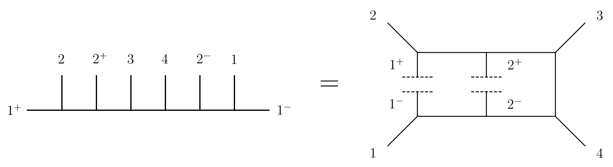
Let us test the strategy at two loops, for which the BCJ representation of the four-point supergravity loop integrand is long known Bern et al. 1998 77 7 The known result is for 4D supergravity. The 10D type II supergravity amplitude is not defined, due to the UV divergence, but the loop integrand can be taken to be a straightforward dimensional ‘oxidation’, with appropriate prefactor .. The two-loop BCJ numerators can be compactly written as
| (15) |
They correspond to half-ladder diagrams with loop momenta at the ends; see FIG. 2. A standard two-loop diagram is then obtained by gluing the nodal legs, i.e. with . Taking the result (15) from the literature, it is possible to obtain via (14). Then, it is both natural and easy to rewrite in the form (12), which as explained earlier can be uplifted to genus 2, matching the superstring result . This achieves step (iii).
IV Three Loops
We now apply our strategy to the much more intricate three-loop case. From the general form of a three-loop field theory integrand, namely the inclusion of the relevant diagram topologies, we can determine and . However, they do not appear in (14), so they are not important for the goal of this paper 88 8 They will be discussed elsewhere.. The important quantities are and . The Jacobian is straightforwardly obtained from (7) and can be written as
| (16) |
where in the factor
| (17) |
the subscript refers to hyperelliptic, as we will explain.
We can now determine using (14). The right-hand side is obtained from the known BCJ representation of the three-loop supergravity integrand, a landmark application of the double copy Bern et al. 2010 99 9 The result in Bern et al. 2010 applies to 4D supergravity, but we will assume that it ‘oxidates’ trivially to 10D type II supergravity for similar reasons as in the two loop case, given the absence of contributions from odd spin structures.. The BCJ numerators, listed in table I of Bern et al. 2010, are not as simple as at two loops and depend linearly on the loop momenta, e.g. 1010 10 Our convention for the external momenta is that they are incoming, whereas the convention in Bern et al. 2010 was that they are outgoing. This affects the sign of the term linear in the loop momenta.
Via (14), this property implies
| (18) |
where the factors were chosen for later convenience. We write our results already in uplifted form, i.e. for (which we claim is ) instead of its degeneration . To determine , we construct a well-motivated ansatz with the required modular weight of , and fix the coefficients of that ansatz by matching numerically the degeneration limit to (14). This requires expanding in the degeneration parameters the Jacobi theta functions which define various objects, a straightforward if computationally heavy procedure.
The second term in (18) is the easiest: we can write
| (19) |
with . All the ingredients have been introduced previously.
The object is more involved. It is convenient to extricate the kinematic dependence by writing
| (20) |
where is independent of the and is symmetric when exchanging: , , . Let us first state the result and then discuss it:
| (21) |
where
| (22) | ||||
| (23) | ||||
| (24) |
Starting with the expression (IV), the object is the normalised Abelian differential of the third kind, whose degeneration limit is
| (25) |
A consistency check is that the contribution (IV), including the kinematic coefficient, is completely fixed by (19). This follows from the condition of ‘homology invariance’: distinct choices of homology cycles of the Riemann surface with respect to the marked points obey monodromy relations dictated by the chiral splitting procedure D’Hoker and Phong 1989, and this connects the two contributions 1111 11 In summary, if a marked point is shifted by a ‘B-cycle’, (i) the loop momentum associated to that cycle is shifted by and (ii) the Abelian differential of the third kind has non-trivial monodromy. These two effects combine precisely to achieve homology invariance. See the very clear discussion for the two-loop five-point amplitude in D’Hoker et al. 2020, where the objects relate to as .
The contributions (IV) and (24) are more elaborate, but the structure is familiar from the RNS formalism D’Hoker and Phong 1988; D’Hoker and Phong 2002a; D’Hoker and Phong 2002b; D’Hoker and Phong 2002c; D’Hoker and Phong 2002d; D’Hoker and Phong 2002e; D’Hoker and Phong 2005d; D’Hoker and Phong 2005a. The sums are over the 36 even spin structures at genus 3, labelled by , and the objects are the Szegő kernels arising from the OPEs of worldsheet fermions. The ‘chiral measure’ is the crucial ingredient. Here, is a modular form of weight 9 (note our non-standard definition for the sign), defined in terms of the even Jacobi theta functions. The general properties of the chiral measure were described in D’Hoker and Phong 2005c; D’Hoker and Phong 2005b and the precise definition of was given in Cacciatori et al. 2008a. It is a sophisticated definition, so we will not repeat it here; we found ref. Tsuyumine 1986 very helpful. The RNS derivation of this measure remains obscure; see appendix C of Witten 2015.
In the degeneration limit , vanishes with leading behaviour ,
| (26) |
where is given in (17). It is opportune to note that only a codimension-1C subset of genus-3 Riemann surfaces are hyperelliptic (whereas for all surfaces are), and these are precisely identified by the vanishing of 1212 12 and the non-vanishing of another modular form called in the classical reference Igusa 1967.. The condition identifies hyperelliptic surfaces in the degeneration limit. The factors of in and in cancel, such that does not vanish in the hyperelliptic sector.
The sums (IV) and (24), which are modular forms of weight 8, vanish in the degeneration limit in a manner analogous to , so that the ratio appearing in (21) yields a finite result on the nodal sphere 1313 13 One may also ask why a sum with is absent from our result, since it has the correct symmetries. It turns out that this sum gives precisely twice the sum (24), at least in the degeneration limit (we expect this to hold beyond the limit too).. As consistency checks on our implementation of the chiral measure, we verified to order the following identities (respectively, from Cacciatori et al. 2008a; Grushevsky and Salvati Manni 2010; Matone and Volpato 2009):
where we determined the previously unknown coefficient . We could not find simplified expressions for (IV) and (24); they are not proportional to , i.e. not proportional to in the degeneration limit.
Comparing our result to the pure spinor computation of Gomez and Mafra 2013, the latter was restricted to part of the correlator and was not manifestly modular invariant, but appears to be consistent at least with (19). The main goal of Gomez and Mafra 2013, for which the partial computation was sufficient, was to match a prediction from S-duality Green and Vanhove 2006 for the low-energy amplitude, where the overall normalisation is important. We neglected the normalisation here, and leave this aspect and a proper comparison to Gomez and Mafra 2013 for future work. Due to manifest supersymmetry, the splitting of spin structures does not arise in the pure spinor approach Berkovits 2000; Berkovits 2001; Berkovits 2003; Berkovits 2004; Berkovits 2006; Berkovits and Mafra 2006, so this approach may be helpful in simplifying the sums seen above.
V Discussion
We have constructed a conjectured expression for the three-loop four-point amplitude of massless states in the type II superstring. The crucial ingredient is the chiral half-integrand (18). As at two loops D’Hoker and Phong 2005a; D’Hoker et al. 2020, this object can also in principle be imported into the Heterotic superstring, paired with a bosonic counterpart.
In place of a first-principles worldsheet calculation, we wrote down an ansatz inspired by insights from the RNS and pure spinor formalisms, and then constrained that ansatz using supergravity data mined with modern amplitudes techniques. Our focus was on briefly delineating a strategy, with very concrete results. Additional technical details will be presented elsewhere. We hope that our conjecture can guide rigorous derivations using established worldsheet methods. Alternatively, in the spirit of the amplitudes programme, perhaps the proof can follow from a set of basic constraints, such as unitarity.
Natural future directions are: the study of the moduli-space integration in the low-energy limit, building on D’Hoker et al. 2005; Gomez and Mafra 2013; D’Hoker and Green 2013; D’Hoker et al. 2015; D’Hoker et al. 2021, which is newly motivated by beautiful advances in the non-perturbative amplitudes bootstrap Guerrieri et al. 2021; and the consideration of higher-point Tsuchiya 1989; Richards 2008; Mafra and Schlotterer 2014; Tsuchiya 2012; Green et al. 2013; Mafra and Schlotterer 2015a; Mafra and Schlotterer 2015b; Mafra and Schlotterer 2016; Mafra and Schlotterer 2019a; Mafra and Schlotterer 2019b; Mafra and Schlotterer 2019c; D’Hoker et al. 2020; D’Hoker et al. 2021 or higher-loop D’Hoker and Phong 2005b; Cacciatori et al. 2008a; Grushevsky 2009; Cacciatori et al. 2008b; Salvati-Manni 2008; Morozov 2008; Grushevsky and Salvati Manni 2011; Matone and Volpato 2010; Matone and Volpato 2006 amplitudes. We expect our strategy to prove useful, not least because there are BCJ numerators for supergravity up to five loops Bern et al. 2012; Bern et al. 2017a; Bern et al. 2017b, although the five-loop case required a generalisation of this representation. Also at this loop order, the relation between supermoduli space and ordinary moduli space becomes more intricate Donagi and Witten 2015, calling into question the structure of our starting point (II). The interplay between field theory and string theory amplitudes continues to present us with many challenges and fruitful surprises.
Note As this work was concluded, it came to our knowledge that the authors of D’Hoker et al. 2020 have independently constructed the contribution to the half-integrand that is linear in the loop momenta, equation (19).
Acknowledgements.
Acknowledgements We thank Eric D’Hoker, Carlos Mafra, Boris Pioline, Rodolfo Russo, Oliver Schlotterer and Edward Witten for comments. YG is supported by the CUniverse research promotion project “Toward World-class Fundamental Physics” of Chulalongkorn University (grant CUAASC). RM and RSM are supported by the Royal Society via a University Research Fellowship and a Studentship Grant, respectively.References
- Veneziano (1968) G. Veneziano, Construction of a crossing - symmetric, Regge behaved amplitude for linearly rising trajectories, Nuovo Cim. A 57, 190 (1968).
- Green and Schwarz (1982) M. B. Green and J. H. Schwarz, Supersymmetrical String Theories, Phys. Lett. B 109, 444 (1982).
- Schwarz (1982) J. H. Schwarz, Superstring Theory, Phys. Rept. 89, 223 (1982).
- D’Hoker and Phong (2005a) E. D’Hoker and D. H. Phong, Two-loop superstrings VI: Non-renormalization theorems and the 4-point function, Nucl. Phys. B715, 3 (2005a), arXiv:hep-th/0501197 [hep-th] .
- Berkovits (2006) N. Berkovits, Super-Poincare Covariant Two-Loop Superstring Amplitudes, JHEP 01, 005, arXiv:hep-th/0503197 [hep-th] .
- Berkovits and Mafra (2006) N. Berkovits and C. R. Mafra, Equivalence of Two-Loop Superstring Amplitudes in the Pure Spinor and RNS Formalisms, Phys. Rev. Lett. 96, 011602 (2006), arXiv:hep-th/0509234 [hep-th] .
- D’Hoker and Phong (2005b) E. D’Hoker and D. H. Phong, Asyzygies, modular forms, and the superstring measure II, Nucl. Phys. B 710, 83 (2005b), arXiv:hep-th/0411182 .
- D’Hoker and Phong (2005c) E. D’Hoker and D. H. Phong, Asyzygies, modular forms, and the superstring measure. I., Nucl. Phys. B 710, 58 (2005c), arXiv:hep-th/0411159 .
- Cacciatori et al. (2008a) S. L. Cacciatori, F. Dalla Piazza, and B. van Geemen, Modular Forms and Three Loop Superstring Amplitudes, Nucl. Phys. B 800, 565 (2008a), arXiv:0801.2543 [hep-th] .
- Gomez and Mafra (2013) H. Gomez and C. R. Mafra, The closed-string 3-loop amplitude and S-duality, JHEP 10, 217, arXiv:1308.6567 [hep-th] .
- Green et al. (1982) M. B. Green, J. H. Schwarz, and L. Brink, N=4 Yang-Mills and N=8 Supergravity as Limits of String Theories, Nucl. Phys. B198, 474 (1982).
- Bern et al. (2010) Z. Bern, J. J. M. Carrasco, and H. Johansson, Perturbative Quantum Gravity as a Double Copy of Gauge Theory, Phys.Rev.Lett. 105, 061602 (2010), arXiv:1004.0476 [hep-th] .
- Green et al. (1988) M. B. Green, J. H. Schwarz, and E. Witten, SUPERSTRING THEORY. VOL. 1: INTRODUCTION, Cambridge Monographs on Mathematical Physics (1988).
- (14) Beyond three loops, the integration over the period matrix must be restricted due to the Schottky problem. Beyond four loops, the delicate issue of non-projectedness of supermoduli space is also known to arise Donagi and Witten 2015.
- D’Hoker and Phong (1988) E. D’Hoker and D. H. Phong, The Geometry of String Perturbation Theory, Rev. Mod. Phys. 60, 917 (1988).
- D’Hoker and Phong (1989) E. D’Hoker and D. H. Phong, Conformal Scalar Fields and Chiral Splitting on Superriemann Surfaces, Commun. Math. Phys. 125, 469 (1989).
- (17) This follows from supersymmetry and is clear if we consider factorisable NS-NS external states . The supersymmetric pre-factor is , where is the pre-factor for the open superstring and includes products . At three loops and four points, a 10D Levi-Civita tensor arising from an odd spin structure’s zero mode may just about be saturated: , but it would never give rise to any . Moreover, the contraction of the two Levi-Civita tensors (with and with ) over three indices after loop integration, required for a potentially non-vanishing contribution, yields products , inconsistent with . This discussion is consistent with the results of Gomez and Mafra 2013; Berkovits 2007.
- Cachazo et al. (2014a) F. Cachazo, S. He, and E. Y. Yuan, Scattering of Massless Particles in Arbitrary Dimensions, Phys.Rev.Lett. 113, 171601 (2014a), arXiv:1307.2199 [hep-th] .
- Cachazo et al. (2014b) F. Cachazo, S. He, and E. Y. Yuan, Scattering of Massless Particles: Scalars, Gluons and Gravitons, JHEP 1407, 033, arXiv:1309.0885 [hep-th] .
- Witten (2004) E. Witten, Perturbative gauge theory as a string theory in twistor space, Commun.Math.Phys. 252, 189 (2004), arXiv:hep-th/0312171 [hep-th] .
- Roiban et al. (2004) R. Roiban, M. Spradlin, and A. Volovich, On the tree level S matrix of Yang-Mills theory, Phys.Rev. D70, 026009 (2004), arXiv:hep-th/0403190 [hep-th] .
- Adamo et al. (2014) T. Adamo, E. Casali, and D. Skinner, Ambitwistor strings and the scattering equations at one loop, JHEP 1404, 104, arXiv:1312.3828 [hep-th] .
- Casali and Tourkine (2015) E. Casali and P. Tourkine, Infrared behaviour of the one-loop scattering equations and supergravity integrands, JHEP 1504, 013, arXiv:1412.3787 [hep-th] .
- Adamo and Casali (2015) T. Adamo and E. Casali, Scattering equations, supergravity integrands, and pure spinors, JHEP 1505, 120, arXiv:1502.06826 [hep-th] .
- Geyer et al. (2015) Y. Geyer, L. Mason, R. Monteiro, and P. Tourkine, Loop Integrands for Scattering Amplitudes from the Riemann Sphere, Phys. Rev. Lett. 115, 121603 (2015), arXiv:1507.00321 [hep-th] .
- Geyer et al. (2016a) Y. Geyer, L. Mason, R. Monteiro, and P. Tourkine, One-loop amplitudes on the Riemann sphere, JHEP 03, 114, arXiv:1511.06315 [hep-th] .
- Geyer et al. (2016b) Y. Geyer, L. Mason, R. Monteiro, and P. Tourkine, Two-Loop Scattering Amplitudes from the Riemann Sphere, Phys. Rev. D94, 125029 (2016b), arXiv:1607.08887 [hep-th] .
- Geyer and Monteiro (2018a) Y. Geyer and R. Monteiro, Two-Loop Scattering Amplitudes from Ambitwistor Strings: from Genus Two to the Nodal Riemann Sphere, JHEP 11, 008, arXiv:1805.05344 [hep-th] .
- Mason and Skinner (2014) L. Mason and D. Skinner, Ambitwistor strings and the scattering equations, JHEP 1407, 048, arXiv:1311.2564 [hep-th] .
- (30) For the delta functions, we use the definition , standard in this context.
- (31) is associated to the genus-2 fundamental domain constraint . In particular, arises from relaxing this constraint when degenerating to the sphere Geyer and Monteiro 2018a.
- Tourkine (2017) P. Tourkine, Tropical Amplitudes, Annales Henri Poincare 18, 2199 (2017), arXiv:1309.3551 [hep-th] .
- Bern et al. (2008) Z. Bern, J. Carrasco, and H. Johansson, New Relations for Gauge-Theory Amplitudes, Phys.Rev. D78, 085011 (2008), arXiv:0805.3993 [hep-ph] .
- (34) It should be noted that the supergravity loop integrand in (4), once the moduli-space integral is performed, is not written in terms of Feynman-like propagators, as in the original BCJ representation Bern et al. 2010. It is instead written in an alternative representation, which was discovered in the ambitwistor string; see Geyer et al. 2015; He and Yuan 2015; Baadsgaard et al. 2016; Geyer et al. 2016a; Cachazo et al. 2016; He and Schlotterer 2017; Feng 2016; He et al. 2018; Geyer and Monteiro 2018b; Geyer et al. 2019; Edison et al. 2020; Farrow et al. 2020 for discussions. The supergravity BCJ numerators relevant in our two- and three-loop problems are valid in both representations.
- Bern et al. (2019) Z. Bern, J. J. Carrasco, M. Chiodaroli, H. Johansson, and R. Roiban, The Duality Between Color and Kinematics and its Applications, (2019), arXiv:1909.01358 [hep-th] .
- Kawai et al. (1986) H. Kawai, D. C. Lewellen, and S. H. H. Tye, A Relation Between Tree Amplitudes of Closed and Open Strings, Nucl. Phys. B269, 1 (1986).
- Bjerrum-Bohr et al. (2009) N. E. J. Bjerrum-Bohr, P. H. Damgaard, and P. Vanhove, Minimal Basis for Gauge Theory Amplitudes, Phys. Rev. Lett. 103, 161602 (2009), arXiv:0907.1425 [hep-th] .
- Stieberger (2009) S. Stieberger, Open & Closed vs. Pure Open String Disk Amplitudes, (2009), arXiv:0907.2211 [hep-th] .
- Mafra et al. (2011) C. R. Mafra, O. Schlotterer, and S. Stieberger, Explicit BCJ Numerators from Pure Spinors, JHEP 07, 092, arXiv:1104.5224 [hep-th] .
- Mafra and Schlotterer (2014) C. R. Mafra and O. Schlotterer, The Structure of n-Point One-Loop Open Superstring Amplitudes, JHEP 08, 099, arXiv:1203.6215 [hep-th] .
- Ochirov and Tourkine (2014) A. Ochirov and P. Tourkine, BCJ duality and double copy in the closed string sector, JHEP 05, 136, arXiv:1312.1326 [hep-th] .
- Mafra and Schlotterer (2015a) C. R. Mafra and O. Schlotterer, Towards one-loop SYM amplitudes from the pure spinor BRST cohomology, Fortsch. Phys. 63, 105 (2015a), arXiv:1410.0668 [hep-th] .
- He et al. (2016) S. He, R. Monteiro, and O. Schlotterer, String-inspired BCJ numerators for one-loop MHV amplitudes, JHEP 01, 171, arXiv:1507.06288 [hep-th] .
- Mafra and Schlotterer (2015b) C. R. Mafra and O. Schlotterer, Berends-Giele recursions and the BCJ duality in superspace and components, (2015b), arXiv:1510.08846 [hep-th] .
- Tourkine and Vanhove (2016) P. Tourkine and P. Vanhove, Higher-loop amplitude monodromy relations in string and gauge theory, Phys. Rev. Lett. 117, 211601 (2016), arXiv:1608.01665 [hep-th] .
- Hohenegger and Stieberger (2017) S. Hohenegger and S. Stieberger, Monodromy Relations in Higher-Loop String Amplitudes, Nucl. Phys. B925, 63 (2017), arXiv:1702.04963 [hep-th] .
- Ochirov et al. (2017) A. Ochirov, P. Tourkine, and P. Vanhove, One-loop monodromy relations on single cuts, JHEP 10, 105, arXiv:1707.05775 [hep-th] .
- Tourkine (2020) P. Tourkine, Integrands and loop momentum in string and field theory, Phys. Rev. D 102, 026006 (2020), arXiv:1901.02432 [hep-th] .
- Mizera (2020a) S. Mizera, Aspects of Scattering Amplitudes and Moduli Space Localization, Ph.D. thesis, Princeton, Inst. Advanced Study (2020a), arXiv:1906.02099 [hep-th] .
- Casali et al. (2019) E. Casali, S. Mizera, and P. Tourkine, Monodromy relations from twisted homology, JHEP 12, 087, arXiv:1910.08514 [hep-th] .
- Casali et al. (2021) E. Casali, S. Mizera, and P. Tourkine, Loop amplitudes monodromy relations and color-kinematics duality, JHEP 03, 048, arXiv:2005.05329 [hep-th] .
- Borsten et al. (2021) L. Borsten, H. Kim, B. Jurčo, T. Macrelli, C. Saemann, and M. Wolf, Double Copy from Homotopy Algebras, (2021), arXiv:2102.11390 [hep-th] .
- Bridges and Mafra (2021) E. Bridges and C. R. Mafra, Local BCJ numerators for ten-dimensional SYM at one loop, (2021), arXiv:2102.12943 [hep-th] .
- (54) The tree-level () version of this relation was revealed in string theory in Mafra et al. 2013; Mafra et al. 2011 and in the scattering equations (CHY) formalism in Cachazo et al. 2014b; see also Azevedo et al. 2018; He et al. 2019. Our higher-loop formula is motivated by its verification at two loops in Geyer et al. 2019. The higher-multiplicity extension is trivial.
- Bjerrum-Bohr et al. (2014) N. E. J. Bjerrum-Bohr, P. H. Damgaard, P. Tourkine, and P. Vanhove, Scattering Equations and String Theory Amplitudes, Phys. Rev. D 90, 106002 (2014), arXiv:1403.4553 [hep-th] .
- Mizera (2020b) S. Mizera, Kinematic Jacobi Identity is a Residue Theorem: Geometry of Color-Kinematics Duality for Gauge and Gravity Amplitudes, Phys. Rev. Lett. 124, 141601 (2020b), arXiv:1912.03397 [hep-th] .
- Kalyanapuram (2021a) N. Kalyanapuram, Ambitwistor Integrands from Tensionless Chiral Superstring Integrands, (2021a), arXiv:2103.07943 [hep-th] .
- Kalyanapuram (2021b) N. Kalyanapuram, On Chiral Splitting and the Ambitwistor String, (2021b), arXiv:2103.08584 [hep-th] .
- Bern et al. (1998) Z. Bern, L. J. Dixon, D. C. Dunbar, M. Perelstein, and J. S. Rozowsky, On the relationship between Yang-Mills theory and gravity and its implication for ultraviolet divergences, Nucl. Phys. B530, 401 (1998), arXiv:hep-th/9802162 [hep-th] .
- (60) The known result is for 4D supergravity. The 10D type II supergravity amplitude is not defined, due to the UV divergence, but the loop integrand can be taken to be a straightforward dimensional ‘oxidation’, with appropriate prefactor .
- (61) They will be discussed elsewhere.
- (62) The result in Bern et al. 2010 applies to 4D supergravity, but we will assume that it ‘oxidates’ trivially to 10D type II supergravity for similar reasons as in the two loop case, given the absence of contributions from odd spin structures.
- (63) Our convention for the external momenta is that they are incoming, whereas the convention in Bern et al. 2010 was that they are outgoing. This affects the sign of the term linear in the loop momenta.
- (64) In summary, if a marked point is shifted by a ‘B-cycle’, (i) the loop momentum associated to that cycle is shifted by and (ii) the Abelian differential of the third kind has non-trivial monodromy. These two effects combine precisely to achieve homology invariance. See the very clear discussion for the two-loop five-point amplitude in D’Hoker et al. 2020, where the objects relate to as .
- D’Hoker and Phong (2002a) E. D’Hoker and D. H. Phong, Lectures on two loop superstrings, Superstring theory. Proceedings, International Conference, Hangzhou, P.R. China, August 12-15, 2002, Conf. Proc. C0208124, 85 (2002a), [,85(2002)], arXiv:hep-th/0211111 [hep-th] .
- D’Hoker and Phong (2002b) E. D’Hoker and D. H. Phong, Two loop superstrings. 1. Main formulas, Phys. Lett. B529, 241 (2002b), arXiv:hep-th/0110247 [hep-th] .
- D’Hoker and Phong (2002c) E. D’Hoker and D. H. Phong, Two loop superstrings. 2. The Chiral measure on moduli space, Nucl. Phys. B636, 3 (2002c), arXiv:hep-th/0110283 [hep-th] .
- D’Hoker and Phong (2002d) E. D’Hoker and D. H. Phong, Two loop superstrings. 3. Slice independence and absence of ambiguities, Nucl. Phys. B636, 61 (2002d), arXiv:hep-th/0111016 [hep-th] .
- D’Hoker and Phong (2002e) E. D’Hoker and D. H. Phong, Two loop superstrings 4: The Cosmological constant and modular forms, Nucl. Phys. B639, 129 (2002e), arXiv:hep-th/0111040 [hep-th] .
- D’Hoker and Phong (2005d) E. D’Hoker and D. H. Phong, Two-loop superstrings. V. Gauge slice independence of the N-point function, Nucl. Phys. B715, 91 (2005d), arXiv:hep-th/0501196 [hep-th] .
- Tsuyumine (1986) S. Tsuyumine, On Siegel modular forms of degree three, Amer. J. Math. 108, 755 (1986).
- Witten (2015) E. Witten, The Super Period Matrix With Ramond Punctures, J. Geom. Phys. 92, 210 (2015), arXiv:1501.02499 [hep-th] .
- (73) And the non-vanishing of another modular form called in the classical reference Igusa 1967.
- (74)
One may also ask why a sum with
is absent from our result, since it has the correct symmetries. It turns out that this sum gives precisely twice the sum (24), at least in the degeneration limit (we expect this to hold beyond the limit too). - Grushevsky and Salvati Manni (2010) S. Grushevsky and R. Salvati Manni, The Vanishing of two-point functions for three-loop superstring scattering amplitudes, Commun. Math. Phys. 294, 343 (2010), arXiv:0806.0354 [hep-th] .
- Matone and Volpato (2009) M. Matone and R. Volpato, Superstring measure and non-renormalization of the three-point amplitude, Nucl. Phys. B 806, 735 (2009), arXiv:0806.4370 [hep-th] .
- Green and Vanhove (2006) M. B. Green and P. Vanhove, Duality and higher derivative terms in M theory, JHEP 01, 093, arXiv:hep-th/0510027 .
- Berkovits (2000) N. Berkovits, Super Poincare covariant quantization of the superstring, JHEP 04, 018, arXiv:hep-th/0001035 .
- Berkovits (2001) N. Berkovits, Covariant quantization of the superparticle using pure spinors, JHEP 09, 016, arXiv:hep-th/0105050 .
- Berkovits (2003) N. Berkovits, ICTP lectures on covariant quantization of the superstring, ICTP Lect. Notes Ser. 13, 57 (2003), arXiv:hep-th/0209059 .
- Berkovits (2004) N. Berkovits, Multiloop amplitudes and vanishing theorems using the pure spinor formalism for the superstring, JHEP 09, 047, arXiv:hep-th/0406055 .
- D’Hoker et al. (2020) E. D’Hoker, C. R. Mafra, B. Pioline, and O. Schlotterer, Two-loop superstring five-point amplitudes. Part I. Construction via chiral splitting and pure spinors, JHEP 08, 135, arXiv:2006.05270 [hep-th] .
- D’Hoker et al. (2005) E. D’Hoker, M. Gutperle, and D. H. Phong, Two-loop superstrings and S-duality, Nucl. Phys. B722, 81 (2005), arXiv:hep-th/0503180 [hep-th] .
- D’Hoker and Green (2013) E. D’Hoker and M. B. Green, Zhang-Kawazumi Invariants and Superstring Amplitudes, (2013), arXiv:1308.4597 [hep-th] .
- D’Hoker et al. (2015) E. D’Hoker, M. B. Green, B. Pioline, and R. Russo, Matching the interaction at two-loops, JHEP 01, 031, arXiv:1405.6226 [hep-th] .
- D’Hoker et al. (2021) E. D’Hoker, C. R. Mafra, B. Pioline, and O. Schlotterer, Two-loop superstring five-point amplitudes. Part II. Low energy expansion and S-duality, JHEP 02, 139, arXiv:2008.08687 [hep-th] .
- Guerrieri et al. (2021) A. Guerrieri, J. Penedones, and P. Vieira, Where is String Theory?, (2021), arXiv:2102.02847 [hep-th] .
- Tsuchiya (1989) A. Tsuchiya, More on One Loop Massless Amplitudes of Superstring Theories, Phys. Rev. D39, 1626 (1989).
- Richards (2008) D. M. Richards, The One-Loop Five-Graviton Amplitude and the Effective Action, JHEP 10, 042, arXiv:0807.2421 [hep-th] .
- Tsuchiya (2012) A. G. Tsuchiya, On the pole structures of the disconnected part of hyper elliptic g loop M point super string amplitudes, (2012), arXiv:1209.6117 [hep-th] .
- Green et al. (2013) M. B. Green, C. R. Mafra, and O. Schlotterer, Multiparticle one-loop amplitudes and S-duality in closed superstring theory, JHEP 10, 188, arXiv:1307.3534 [hep-th] .
- Mafra and Schlotterer (2016) C. R. Mafra and O. Schlotterer, One-loop superstring six-point amplitudes and anomalies in pure spinor superspace, JHEP 04, 148, arXiv:1603.04790 [hep-th] .
- Mafra and Schlotterer (2019a) C. R. Mafra and O. Schlotterer, Towards the n-point one-loop superstring amplitude. Part I. Pure spinors and superfield kinematics, JHEP 08, 090, arXiv:1812.10969 [hep-th] .
- Mafra and Schlotterer (2019b) C. R. Mafra and O. Schlotterer, Towards the n-point one-loop superstring amplitude. Part II. Worldsheet functions and their duality to kinematics, JHEP 08, 091, arXiv:1812.10970 [hep-th] .
- Mafra and Schlotterer (2019c) C. R. Mafra and O. Schlotterer, Towards the n-point one-loop superstring amplitude. Part III. One-loop correlators and their double-copy structure, JHEP 08, 092, arXiv:1812.10971 [hep-th] .
- Grushevsky (2009) S. Grushevsky, Superstring scattering amplitudes in higher genus, Commun. Math. Phys. 287, 749 (2009), arXiv:0803.3469 [hep-th] .
- Cacciatori et al. (2008b) S. L. Cacciatori, F. Dalla Piazza, and B. van Geemen, Genus four superstring measures, Lett. Math. Phys. 85, 185 (2008b), arXiv:0804.0457 [hep-th] .
- Salvati-Manni (2008) R. Salvati-Manni, Remarks on Superstring amplitudes in higher genus, Nucl. Phys. B 801, 163 (2008), arXiv:0804.0512 [hep-th] .
- Morozov (2008) A. Morozov, NSR Superstring Measures Revisited, JHEP 05, 086, arXiv:0804.3167 [hep-th] .
- Grushevsky and Salvati Manni (2011) S. Grushevsky and R. Salvati Manni, The superstring cosmological constant and the Schottky form in genus 5, Am. J. Math. 133, 1007 (2011), arXiv:0809.1391 [math.AG] .
- Matone and Volpato (2010) M. Matone and R. Volpato, Getting superstring amplitudes by degenerating Riemann surfaces, Nucl. Phys. B 839, 21 (2010), arXiv:1003.3452 [hep-th] .
- Matone and Volpato (2006) M. Matone and R. Volpato, Higher genus superstring amplitudes from the geometry of moduli space, Nucl. Phys. B 732, 321 (2006), arXiv:hep-th/0506231 .
- Bern et al. (2012) Z. Bern, J. J. M. Carrasco, L. J. Dixon, H. Johansson, and R. Roiban, Simplifying Multiloop Integrands and Ultraviolet Divergences of Gauge Theory and Gravity Amplitudes, Phys. Rev. D 85, 105014 (2012), arXiv:1201.5366 [hep-th] .
- Bern et al. (2017a) Z. Bern, J. J. Carrasco, W.-M. Chen, H. Johansson, and R. Roiban, Gravity Amplitudes as Generalized Double Copies of Gauge-Theory Amplitudes, Phys. Rev. Lett. 118, 181602 (2017a), arXiv:1701.02519 [hep-th] .
- Bern et al. (2017b) Z. Bern, J. J. M. Carrasco, W.-M. Chen, H. Johansson, R. Roiban, and M. Zeng, Five-loop four-point integrand of supergravity as a generalized double copy, Phys. Rev. D96, 126012 (2017b), arXiv:1708.06807 [hep-th] .
- Donagi and Witten (2015) R. Donagi and E. Witten, Supermoduli Space Is Not Projected, Proc. Symp. Pure Math. 90, 19 (2015), arXiv:1304.7798 [hep-th] .
- Berkovits (2007) N. Berkovits, New higher-derivative R**4 theorems, Phys. Rev. Lett. 98, 211601 (2007), arXiv:hep-th/0609006 .
- He and Yuan (2015) S. He and E. Y. Yuan, One-loop Scattering Equations and Amplitudes from Forward Limit, Phys. Rev. D92, 105004 (2015), arXiv:1508.06027 [hep-th] .
- Baadsgaard et al. (2016) C. Baadsgaard, N. E. J. Bjerrum-Bohr, J. L. Bourjaily, S. Caron-Huot, P. H. Damgaard, and B. Feng, New Representations of the Perturbative S-Matrix, Phys. Rev. Lett. 116, 061601 (2016), arXiv:1509.02169 [hep-th] .
- Cachazo et al. (2016) F. Cachazo, S. He, and E. Y. Yuan, One-Loop Corrections from Higher Dimensional Tree Amplitudes, JHEP 08, 008, arXiv:1512.05001 [hep-th] .
- He and Schlotterer (2017) S. He and O. Schlotterer, New Relations for Gauge-Theory and Gravity Amplitudes at Loop Level, Phys. Rev. Lett. 118, 161601 (2017), arXiv:1612.00417 [hep-th] .
- Feng (2016) B. Feng, CHY-construction of Planar Loop Integrands of Cubic Scalar Theory, JHEP 05, 061, arXiv:1601.05864 [hep-th] .
- He et al. (2018) S. He, O. Schlotterer, and Y. Zhang, New BCJ representations for one-loop amplitudes in gauge theories and gravity, Nucl. Phys. B930, 328 (2018), arXiv:1706.00640 [hep-th] .
- Geyer and Monteiro (2018b) Y. Geyer and R. Monteiro, Gluons and gravitons at one loop from ambitwistor strings, JHEP 03, 068, arXiv:1711.09923 [hep-th] .
- Geyer et al. (2019) Y. Geyer, R. Monteiro, and R. Stark-Muchão, Two-Loop Scattering Amplitudes: Double-Forward Limit and Colour-Kinematics Duality, JHEP 12, 049, arXiv:1908.05221 [hep-th] .
- Edison et al. (2020) A. Edison, S. He, O. Schlotterer, and F. Teng, One-loop Correlators and BCJ Numerators from Forward Limits, JHEP 09, 079, arXiv:2005.03639 [hep-th] .
- Farrow et al. (2020) J. A. Farrow, Y. Geyer, A. E. Lipstein, R. Monteiro, and R. Stark-Muchão, Propagators, BCFW recursion and new scattering equations at one loop, JHEP 10, 074, arXiv:2007.00623 [hep-th] .
- Mafra et al. (2013) C. R. Mafra, O. Schlotterer, and S. Stieberger, Complete N-Point Superstring Disk Amplitude I. Pure Spinor Computation, Nucl. Phys. B873, 419 (2013), arXiv:1106.2645 [hep-th] .
- Azevedo et al. (2018) T. Azevedo, M. Chiodaroli, H. Johansson, and O. Schlotterer, Heterotic and bosonic string amplitudes via field theory, JHEP 10, 012, arXiv:1803.05452 [hep-th] .
- He et al. (2019) S. He, F. Teng, and Y. Zhang, String amplitudes from field-theory amplitudes and vice versa, Phys. Rev. Lett. 122, 211603 (2019), arXiv:1812.03369 [hep-th] .
- Igusa (1967) J. Igusa, Modular Forms and Projective Invariants, Amer. J. Math. 89, 817 (1967).