Quantum spatial search in two-dimensional waveguide arrays
Abstract
Continuous-time quantum walks (CTQW) have shown the capability to perform efficiently the spatial search of a marked site on many kinds of graphs. However, most of such graphs are hard to realize in an experimental setting. Here we study CTQW spatial search on a planar triangular lattice by means of both numerical simulations and experiments. The experiments are performed using two-dimensional waveguide arrays fabricated by femtosecond laser pulses, illuminated by coherent light. We show that the retrieval of the marked site by the quantum walker is accomplished with higher probability than the classical counterpart, in a convenient time window placed early in the evolution.
I Introduction
The goal of spatial search algorithms is to find a marked item in a collection of entries, or a database, in the presence of displacement constraints. Such constraints define a topology, i.e. which of the entries are directly connected, and can be modelled as the edges of a graph , whose vertices are the entries of the database. One simple strategy to find the target item is to traverse the graph along its edges, upon defining a classical random walk on the graph vertices. Such strategy would result in an average hitting time, i.e. number of jumps needed to hit the target item, linearly scaling with the number of vertices of Chen and Zhan 2008.
Quantum random walks on graphs exhibit, in general, a different behaviour than their classical counterparts Kempe 2003a; Venegas-Andraca 2012; Childs et al. 2002; Gualtieri et al. 2020. A continuous-time quantum walk (CTQW), for example, spreads on the line quadratically faster than its classical analogue, whereas there are particular graphs, such as the glued-tree graph Childs et al. 2003 where such “speed-up” is even exponential. Because of the close connection between graph traversing and the solution of decision problems, these observations have triggered an intensive research, aiming to assess the possible gain achievable by quantum walks, both in the continuous-Farhi and Gutmann 1998; Childs and Goldstone 2004; Childs 2009; de Falco and Tamascelli 2013; Tamascelli and Zanetti 2014; Tamascelli et al. 2016; Chakraborty et al. 2020; Paris et al. 2021 and in the discrete-time Aharonov et al. 1993; Kempe 2003b; Shenvi et al. 2003; Lovett et al. 2010; Koch and Hillery 2018 setting. Spatial search on graphs by means of CTQWs has been thoroughly investigated in the last decades. Differently from a quantum transport setting, which focuses on moving a localized walker from one input site to a target one, in a spatial search the initial state of a search protocol is a uniform distribution over all the sites of the graph, indicating unbiasedness toward the target state. Moreover, an oracle is necessary in quantum search to correctly identify the solution node, while this is not required in transport where the target vertex is well identified. Starting from the seminal work from Childs and Goldstone Childs and Goldstone 2004, the advantage provided by CTQW to quantum spatial search on different families of graphs has been analyzed Childs and Ge 2014; Meyer and Wong 2015; Philipp et al. 2016; Chakraborty et al. 2016; Osada et al. 2018; Glos and Januszek 2019; Osada et al. 2020; Portugal 2018.
Implementing the spatial search algorithm in experiments is not trivial. To realize a CTQW, an experimental system has to be realized where a quantum particle can tunnel among the sites of a network, which are interconnected by some physical interaction. However, the simplest versions of the spatial search algorithm based on CTQW finds the target with unit probability only for spatial dimensions equal or larger than 4 (hypercube), or for fully-connected graphs Childs and Goldstone 2004. Since physical interactions rapidly decay with the distance, it is hard to implement a physical system of quantum sites with such a high degree of connectivity. Variations of the original algorithm have been shown to work efficiently also for two-dimensional graphs with Dirac points in the spectrum Foulger et al. 2014; Childs and Ge 2014, such as honeycomb graphs. Other algorithms, working in two-dimensional graphs such as triangular ones, require on the other hand discrete-time quantum walks Tulsi 2008; Abal et al. 2012 and pose additional experimental difficulties, such as the implementation of the coin operator and of the conditional shift operator. Whereas a large number of implementations of CTQW for the study of quantum information transfer and diffusion processes in different physical platforms are described in the literature Manouchehri and Wang 2006; Gräfe et al. 2016, a single experiment of CTQW-based spatial search, implementing the spatial search on a honeycomb lattice, has been reported Böhm et al. 2015. Such experiment used classical waves in a microwave setup containing weakly coupled dielectric resonators. In addition, the spatial search algorithm was recently run on a photonic processor Qiang et al. 2021; however, in that case the Hamiltonian was artificially codified in a multi-photon quantum interference experiment.
In this paper, we address the experimental implementation of quantum spatial search on two-dimensional triangular graphs by means of a photonic CTQW. In particular, graphs are encoded in two-dimensional arrays of optical waveguides fabricated by the femtosecond laser writing technique Szameit et al. 2006; Crespi et al. 2012; Feng et al. 2016, while walkers are photons from a coherent continous-waved laser beam. The coherent beam illuminates the input facet of the array, providing a delocalized input state. Optical waveguides, weakly coupled by evanescent-field interaction, represent quantum sites across which photons can tunnel at controlled amplitudes along propagation, and thus provide a convenient setting for implementing a CTQW Perets et al. 2008; Poulios et al. 2014; Caruso et al. 2016; Tang et al. 2018. The photon distribution is retrieved by imaging the output facet of the array onto a CCD camera.
We show that, in the presence of an engineered “defect” marking the target database entry, the walker wave function tends to concentrate at the defect allowing for an identification of the target. To quantify the advantage gained by using CTQW, we introduce and evaluate a suitable figure of merit that takes into account the fact that time is a resource to be used parsimoniously. In particular, we observe that such concentration process is faster than the classical random search on the same graph in a convenient time window.
II The model
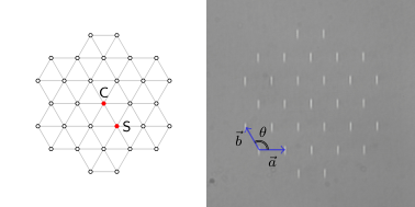
We consider the spatial search problem on finite triangular lattices, i.e. Bravais lattice with parameters (see Fig. 1). The corresponding graph is fully defined by the adjacency matrix , where if and otherwise, and is the number of vertices.
The basis state , of the -dimensional Hilbert space of states , identifies a configuration where a single excitation, or walker, is located at the vertex . The adjacency matrix generates a quantum walk on through the unitary evolution (): , with any initial state in and a constant setting the transition rate of the walker. In order to perform the search of a target vertex , we introduce a local perturbation in the form of a diagonal matrix , with , which acts as an oracle Childs and Goldstone 2004. The quantum Hamiltonian for the search of a target site reads, therefore
| (1) |
We will moreover consider the linear superposition of all the nodes as the initial condition . The probability of finding the walker at the target site at time ,
| (2) |
We note that the parameter governs the overall time-scale of the system dynamics. If one considers a normalized evolution time , the probability will be determined by the ratio .
In order to compare the features of the quantum spatial search with those of a classical random search, we define the following stochastic process on . The dynamics of a classical random walk in the absence of the marked vertex is generated by the graph Laplacian matrix, defined as , where is a diagonal matrix and indicates the degree of the -th vertex.
In order to mark a site and to model the fact that when the process hits the target vertex the search task is completed, we modify the graph by making all the transitions to the marked vertex irreversible. We do that by setting the edges entering into as directed. It follows that the generator of the classical dynamics is determined by the Laplacian of a directed graph, , such that ( is called a sink) and with diagonal entries fixed such that the sum of the elements of each column of is equal to zero, i.e. . In this way, is a proper generator of the trace-preserving semi-group , with the transition rate. For the sake of uniformity, we call the vector describing the initial probability distribution of the classical walker on the graph sites, with the property that . The probability of reaching the target at time is given by:
| (3) |
III Simulation of spatial search by CTQW
We study the spatial search on the finite graph sketched in Fig. 1 composed of 31 sites, and we consider two possible positions for the target: the central site (C) and a site in a shifted position, adjacent to the central one (S). We report in Fig. 2a,b the classical and quantum probability to reach the two different target sites, calculated numerically through Eqs. (2) and (3) respectively.
In order to compute the quantum evolution, we fix in both cases , a value that optimizes the maximum value reached by for a target placed at the centre of the graph. We thus make the target on-site energy independent of its location since, in principle, in a search problem the target location is not known a-priori. As shown in Fig. 3, the qualitative behavior of the target probability presents a smooth dependence, for fixed value of the dimensionless time , on the value of the ratio . It follows that a small detuning in does not significantly degrade the spatial search.
We note that is monotonically increasing in time, because of the irreversible nature of the dynamics described by the generator . Namely, in the classical search as defined in the previous section, the walker always finds the target node if we wait long enough. However, surpasses in both considered cases, for wide time intervals early in the walk evolution.
To provide an immediate comparison of the quantum dynamics versus the classical counterpart, and thus reliable information about the speedup of the quantum search with respect to the classical case, we introduce the ratio of the two probabilities:
| (4) |
In fact, our aim is not only to identify the target node using a CTQW, but also to perform the spatial search in the shortest possible time. Since in the classical case the probability of finding the target is a monotonically increasing function of time, while in the quantum case it has an oscillatory behaviour, naturally takes into account both the fact that we want the to be large and time to be small. Plots of , for the two considered target sites in our finite graph, are reported in panels (c) and (d) of Fig. 2: The orange region highlights the time-intervals where the quantum walker outperforms its classical analogue in finding the target node. Remarkably enough, we do not need to measure the walker position at a specific single time, but we have a large time interval in which the CTQW better identifies the target node with respect to a classical continuous-time random walk, i.e. .
We should note that these results are not specific to the graph of Fig. 1. The qualitative trend of the quantity keeps indeed its validity if we increase the size of the graph. In Appendix A we report the scaling behavior of for a triangular lattice with increasing number of vertices, and we show that there is always an advantage in using a quantum walk to perform the search, with respect to its classical counterpart.


IV Spatial search in a waveguide setting
In our experiments we study the spatial search problem in a photonic setting, exploiting lattices of single-mode waveguides, weakly coupled to each other. Considering only first-neighbour coupling, the dynamics of one photon propagating in the array can be precisely mapped to a single-particle CTQW described by the Hamiltonian (1). In fact, the states represent the occupation of the optical mode of the -th waveguide of the array. Because of evanescent-field coupling, during the propagation the photon can tunnel in neighbouring waveguides with a rate . A detuning in the propagation constant of the -th optical mode implements the parameter . In addition, the evolution time is directly mapped onto the propagation coordinate; indeed, we can take directly the longitudinal spatial coordinate as a measure of the evolution time .
We fabricated lattices of 31 waveguides in fused-silica substrates, with the geometry as in Fig. 1, using the femtosecond laser waveguide writing technique. In detail, we employed a commercial laser system (LightConversion Pharos) providing 180 fs pulses with up to 40 J energy and repetition rates up to 1 MHz. For the waveguide inscription we used a repetition rate of 50 kHz and pulses with 250 nJ energy, which were focused in the bulk of the substrate by means of a 20 (0.45 NA) microscope objective. The average depth of the waveguide arrays below the substrate surface is 170 m, for which the objective provides optimal compensation of spherical aberrations. Individual waveguides sustain a single guided mode at the wavelength of 633 nm, with mode size of about 13 m ( diameter) and propagation loss of about 0.5 dB/cm.

The waveguide arrays were realized with different length and waveguide separation, to provide different values of (see Appendix B). To implement the target site, the correspondent waveguide was inscribed with a different speed with respect to the other ones. In fact, for femtosecond laser written waveguides the coupling coefficient is typically an exponentially decreasing function of the waveguide separation, while the propagation constant can be modulated by varying the writing speed Crespi et al. 2012. We note that, for the inscription parameters adopted in our experiment, mode size and propagation losses are negligibly affected by these changes in writing speed. For a given value of , three kind of arrays were fabricated, one next to the other in the glass: one without target (i.e. with all identical waveguides), one with the target on the site C, one with the target shifted on the site S (see Fig. 1). The nominal ratio was kept fixed to well within the range of values that optimize the search of a target placed at the centre of the graph (see Fig. 3).
To realize the spatial search algorithm, we employed the apparatus sketched in Fig. 4a. To provide a stream of photons at the input, delocalized with (approximately) equal probability amplitude and phase across all the optical modes of the array, we mildly focused a He:Ne laser beam using a = 40 cm convex lens and we placed the input facet of the array in the focal point.
The = 40 cm lens produces a focal spot of about 400 m diameter, experimentally measured with the knife-edge technique, which is larger than the array size. This beam diameter is sufficient to approximate, in our experiments, a uniform excitation; indeed, the output distribution is found experimentally to be marginally affected by small shifts in the transverse alignment of the beam with respect to the center of the array. Besides, a Gaussian beam yields a planar wavefront in its waist and such planar phase condition is maintained with good approximation in the Rayleigh region, which in this case is a few centimeters long. Thus, also the longitudinal positioning of the glass chip is not critical. On the other hand, the tilt degrees of freedom need to be carefully adjusted: if the propagation vector of the impinging beam is not parallel to the propagation vector of the optical modes of the array, a phase gradient results to be imposed to the input state, with possible severe consequences on the evolution (see Appendix C and Fig. 9).
Output light was collected with a 10 (0.25 NA) microscope objective and imaged onto a monochromatic CCD camera. The pixel intensities are proportional to the average photon number impinging on the pixel area. We note that the output photon distribution measured by our experimental setup is identical to the one obtainable using pure single-photon sources at the input, and single-photon-sensitive imaging devices at the output.
V Experimental results
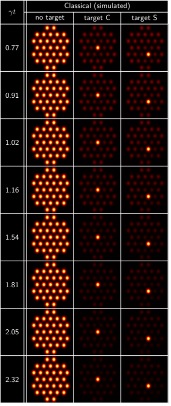
Experimental images of the output light distribution, for all the fabricated waveguide arrays, are reported in Fig. 4b. The figure also shows, for comparison, the results of numerical simulation, performed considering the nominal values for the normalized time and for the ratio in each array. Simulations also assumed an ideal flat input wavefront. The simulated distribution of a classical random walker in analogous conditions is given, as a further comparison, in Fig. 10.
Figure 5 reports the occupation probability for each waveguide, obtained from the images in Fig. 4b. In detail, to retrieve these values the pixel intensities were integrated within circles of about the size of the optical modes, centered on the position of each waveguide. The obtained distribution was then normalized to sum up to one. We note that the optical losses of the waveguides, which are uniform across the array, do not influence the normalized distribution.
From both figures we can observe a clear concentration of the light on the target waveguide (in the arrays where a target is implemented) for quite a wide range of values of . Importantly, in a large part of the investigated time interval, the probability to find a photon in the target waveguide is dominant over the correspondent probability for a classical walker to have reached that site. Thus the ratio , estimated by combining the result of the experimental measurements for the CTQW, and numerical simulations of the classical case, robustly exceeds one for both target positions.
Some light concentration in the central waveguide is also observed in the case of shifted target and even in the case of the uniform arrays, at evolution times (see Fig. 4). We attribute this to boundary effects, i.e. to the partial reflection of the delocalized initial state from the edges of the finite-sized lattice, which tends to focus in the middle at certain evolution times. The occurrence of this spurious focusing effect, which influences the convergence of the spatial search algorithm, explains why the target is reached with higher probability when this is placed in the central position with respect to the case in which it is shifted.
The differences between the simulated and measured distributions, which are noted in Figs. 4b and Fig. 5, may be due to contributions from several causes. For instance, the fabrication technique presents tolerances in implementing the desired values of coupling coefficients and detuning . In particular, the experimental laws that relate these quantities to the inter-waveguide distance and to the writing speed are crucially dependent on the microscopic refractive index distribution of the waveguide, which in turn is a result of complex interactions between the laser pulses and the substrate. Drifts in the performance of the femtosecond laser used for the fabrication (e.g. in the pulse length), may cause these laws to change slightly from day to day, with respect to the preliminary calibration. As a matter of fact, these non-idealities do not prevent the observation of a favourable localization of the quantum walker on the target, as discussed above.
VI Conclusion and Outlook
We have experimentally demonstrated the spatial search algorithm on a finite-size triangular graph, exploiting two-dimensional waveguide arrays and coherent light excitation. The target site was encoded as an engineered defect in the lattice. We have shown that there is a relevant time window in which the walker wavefunction concentrates at the target site with higher probability than the corresponding classical random search on the same graph.
We have therefore provided evidence that 2D graphs, while not optimal, are able to achieve interesting results with a reasonable experimental effort. In particular, we have shown that the quantum advantage is clear also with these topologies, especially in comparison with a classical random walk search, without the need to implement a fully connected graph.
Our results are particularly interesting in any situation where time is a constrained resource, and the database corresponds to a poorly connected structure. In those cases, in fact, finding the target with certainty is impossible with classical resources, and no simple quantum algorithms are available. Indeed, we have found that a simple CTQW may provide an advantage over the classical counterpart, in identifying the target with larger probability.
This study provides an experimental implementation of the CTQW spatial-search algorithm in a photonic system, where the quantum walk dynamics is effectively reproduced in an analogical setting. Optical waveguide arrays are indeed a highly versatile platform, which may allow in the future to explore not only different graph geometries, such as square or hexagonal lattices, but also to implement different search protocols, as the vacancy-based search scheme proposed in Foulger et al. 2014.
In addition, we observe that the search problem stated through Eq. (1) can be reinterpreted as a strategy to identify defects in physical systems. The projector onto the target state modifies the on-site energy of a particular vertex by a detuning , being akin to the effect of a fabrication defect in a lattice. As shown in our numerical simulations, the localization effect is robust with respect to variations in . Therefore, a CTQW which starts in a superposition of all sites may be used to detect the flawed node, i.e. the target site.
Acknowledgements
DT has been supported by UniMi through the “Sviluppo UniMi” initiative. AC acknowledges funding by the Ministero dell’Istruzione, dell’Università e della Ricerca (PRIN 2017 progamme, QUSHIP project - id. 2017SRNBRK). MGAP is member of INdAM-GNFM. The Authors would like to thank Dr. Roberto Osellame for helpful discussions.
Appendix A Scaling behaviour of the quantum search


In this section we show that the quantum advantage found in Section III
through the quantity is still valid when the size of the graph is increased, i.e. the number of nodes gets larger.
We consider finite-size triangular lattices, as sketched in Figure 6.
The number of nodes is increased by adding new external layers of vertices.
We focus on three positions for the target node: the central one (C), nearest neighbour to the target (1N) and second-neighbor to the target (2N).
Due to the symmetry of the considered topology, it is always possible to unequivocally identify the central target C and, in turn, its 1N and 2N nodes.
In Figure 7, we report the behaviour of the maximum value of the ratio over time, i.e.
| (5) |
We call the optimal time. As the number of nodes is increased, remains larger than 1, indicating an advantage of the quantum search over the classical analogue (Fig. 7a); on the other hand, the optimal time increases with larger sizes of the lattice (Fig. 7b). The sudden drop in is due to the presence of two competitive peaks in , independently on the target. As becomes large enough, the absolute maximum is reached at shorter times.
In Fig. 7c, we also show the behaviors of the quantum (blue) and classical (orange) target probabilities at the optimal time. Their values decreases with increasing , but the probability of identifying the target with a quantum walker is always larger than with a classical walk. In Figure 8 we display the optimal value of as a function of the target detuning and of the increasing number of graph nodes , for the three target sites considered. The quantum advantage, as quantified by , is robust with respect to variations in throughout a wide region in the parameter-space, thus indicating that there is no need to precisely select a single optimal value for the detuning in Eq. (1).
Appendix B Details of the fabricated waveguide arrays
Waveguide arrays were inscribed in a 60 mm long fused-silica chip, according to the four sets of parameters (A, B, C, D) listed in Table 1. As mentioned in Section IV , three arrays were realized for each of these set of parameters: one without target (i.e. with all identical waveguides), one with the target on the site C, one with the target shifted on the site S. The waveguide separation and inscription speeds and were chosen to give the nominal coupling coefficient and target detuning (where target is present) listed in the Table, according to preliminary calibration experiments. Note that the nominal ratio is kept fixed to about 4.1.
The glass chip was later cut into two parts, with lengths of about 20 mm and 40 mm respectively. End facets were polished at optical quality (this further removed a few hundreds of microns). In this way, devices were obtained spanning eight different values of the normalized propagation coordinate (ranging from 0.77 to 2.32) as shown in Table 2.
| Type | fabrication parameters |
| |||||
| (m) | (mm/s) | (mm/s) | (1/mm) | (1/mm) | |||
| A | 23.40 | 3.69 | 2.00 | 0.060 | 0.25 | ||
| B | 24.37 | 3.32 | 2.00 | 0.053 | 0.22 | ||
| C | 25.30 | 3.03 | 2.00 | 0.047 | 0.19 | ||
| D | 26.56 | 2.78 | 2.00 | 0.040 | 0.17 | ||
| Type | nominal | |
|---|---|---|
| = 19.3 mm | = 38.6 mm | |
| A | 1.16 | 2.32 |
| B | 1.02 | 2.05 |
| C | 0.91 | 1.81 |
| D | 0.77 | 1.54 |
Appendix C Alignment of the waveguide array with the coherent illumination beam
In order to perform reliable measurements, the waveguide arrays must be accurately aligned with respect to the laser beam, especially in the tilt degrees of freedom. To this purpose, the glass chip was mounted on a multi-axis micrometric manipulator (three translation and two rotation axes) and the alignment was operated according to the following procedure.
As a first thing, one uniform array is selected and centered with respect to the input laser beam. A rough adjustment of the transverse position and inclination of the glass chip is conducted without any collection objective, by overlapping the far-field interference pattern produced by the array output with the far-field spot of the uncoupled light, while maximizing the intensity of the former.
In fact, part of the light focused by the = 40 cm lens is not effectively coupled into the waveguides, but keeps propagating and diverging, first within the glass and then out of it. The light coupled into the waveguides and then exiting at the array output, instead, produces a complex interference pattern in the far-field. On the one side, by micrometrically adjusting the sample transverse position, one can maximize the intensity of such interference pattern and thus optimize the overlap of the impinging wavefront with the optical modes of the array. On the other side, action on the tilt degrees of freedom has the effect of translating the far-field position of the interference pattern. If the latter is overlapped to the spot of the uncoupled light, this means that the uncoupled light has the same average wavevector as the light propagating in the waveguides (and then out of them). Given the symmetry of the array, this also imply that the desired input condition has been reached, with all modes excited with the same phase.
The alignment is completed by placing the collection objective in front of the array output, and by imaging the output facet onto a CCD camera. The sample tilt is now finely tuned in order to achieve the most symmetric output distribution (see also Fig. 9).
Since the arrays are inscribed parallel one to the other, we could observe that, once the tilts are optimized for one device, the alignment can be safely maintained also for the neighbouring ones, which can be coupled by just a rigid translation of the glass sample. Thus, the uniform array serves for alignment purposes, and allows for reliable measurements on the neighbouring two, which are interesting for the spatial search experiment.

References
- Chen and Zhan (2008) H. Chen and F. Zhan, “The expected hitting times for finite Markov chains,” Lin. Alg. Appl. (2008) 2730–2749www.sciencedirect.comwww.elsevier.com/locate/laa 428, 2730–2749 (2008).
- Kempe (2003a) J. Kempe, “Quantum random walks: An introductory overview,” Contemp. Phys. 44, 307–327 (2003a).
- Venegas-Andraca (2012) S. E. Venegas-Andraca, “Quantum walks: a comprehensive review,” Quantum Inf. Proc. 11, 1015–1106 (2012).
- Childs et al. (2002) A. M. Childs, E. Farhi, and S. Gutmann, “An example of the difference between quantum and classical random walks,” Quantum Inf. Proc. 1, 35–43 (2002).
- Gualtieri et al. (2020) V. Gualtieri, C. Benedetti, and M. G. A. Paris, “Quantum-classical dynamical distance and quantumness of quantum walks,” Phys. Rev. A 102, 012201 (2020).
- Childs et al. (2003) A. M. Childs, R. Cleve, E. Deotto, E. Farhi, S. Gutmann, and D. A. Spielman, “Exponential algorithmic speedup by a quantum walk,” in Proceedings of the Thirty-Fifth Annual ACM Symposium on Theory of Computing, STOC ’03 (Association for Computing Machinery, New York, NY, USA, 2003) p. 59–68.
- Farhi and Gutmann (1998) E. Farhi and S. Gutmann, “Quantum computation and decision trees,” Phys. Rev. A 58, 915–928 (1998).
- Childs and Goldstone (2004) A. M. Childs and J. Goldstone, “Spatial search by quantum walk,” Phys. Rev. A 70, 022314 (2004).
- Childs (2009) A. M. Childs, “Universal computation by quantum walk,” Phys. Rev. Lett. 102, 180501 (2009).
- de Falco and Tamascelli (2013) D. de Falco and D. Tamascelli, “Noise-assisted quantum transport and computation,” J. Phys. A: Math. Theor. 46, 225301 (2013).
- Tamascelli and Zanetti (2014) D. Tamascelli and L. Zanetti, “A quantum-walk-inspired adiabatic algorithm for solving graph isomorphism problems,” J. Phys. A: Math. Theor. 47, 325302 (2014).
- Tamascelli et al. (2016) D. Tamascelli, S. Olivares, S. Rossotti, R. Osellame, and M. G. A. Paris, “Quantum state transfer via Bloch oscillations,” Sci. Rep. 6, 26054 (2016).
- Chakraborty et al. (2020) S. Chakraborty, L. Novo, and J. Roland, “Optimality of spatial search via continuous-time quantum walks,” Phys. Rev. A 102, 032214 (2020).
- Paris et al. (2021) M. G. A. Paris, C. Benedetti, and S. Olivares, “Improving quantum search on simple graphs by pretty good structured oracles,” Symmetry 13 (2021) .
- Aharonov et al. (1993) Y. Aharonov, L. Davidovich, and N. Zagury, “Quantum random walks,” Phys. Rev. A 48, 1687–1690 (1993).
- Kempe (2003b) J. Kempe, “Discrete quantum walks hit exponentially faster,” in Approximation, Randomization, and Combinatorial Optimization.. Algorithms and Techniques, edited by S. Arora, K. Jansen, J. D. P. Rolim, and A. Sahai (Springer Berlin Heidelberg, Berlin, Heidelberg, 2003) pp. 354–369.
- Shenvi et al. (2003) N. Shenvi, J. Kempe, and K. B. Whaley, “Quantum random-walk search algorithm,” Phys. Rev. A 67, 052307 (2003).
- Lovett et al. (2010) N. B. Lovett, S. Cooper, M. Everitt, M. Trevers, and V. Kendon, “Universal quantum computation using the discrete-time quantum walk,” Phys. Rev. A 81, 042330 (2010).
- Koch and Hillery (2018) D. Koch and M. Hillery, “Finding paths in tree graphs with a quantum walk,” Phys. Rev. A 97, 012308 (2018).
- Childs and Ge (2014) A. M. Childs and Y. Ge, “Spatial search by continuous-time quantum walks on crystal lattices,” Phys. Rev. A 89, 052337 (2014).
- Meyer and Wong (2015) D. A. Meyer and T. G. Wong, “Connectivity is a poor indicator of fast quantum search,” Phys. Rev. Lett. 114, 110503 (2015).
- Philipp et al. (2016) P. Philipp, L. Tarrataca, and S Boettcher, “Continuous-time quantum search on balanced trees,” Phys. Rev. A 93, 032305 (2016).
- Chakraborty et al. (2016) S. Chakraborty, L. Novo, A. Ambainis, and Y. Omar, “Spatial search by quantum walk is optimal for almost all graphs,” Phys. Rev. Lett. 116, 100501 (2016).
- Osada et al. (2018) T. Osada, K. Sanaka, W. J. Munro, and Kae Nemoto, “Spatial search on a two-dimensional lattice with long-range interactions,” Phys. Rev. A 97, 062319 (2018).
- Glos and Januszek (2019) A. Glos and T. Januszek, “Impact of global and local interaction on quantum spatial search on chimera graph,” Int. J. Quantum Inf. 17, 1950040 (2019).
- Osada et al. (2020) T. Osada, B. Coutinho, Y. Omar, K. Sanaka, W. J. Munro, and K. Nemoto, “Continuous-time quantum-walk spatial search on the bollobás scale-free network,” Phys. Rev. A 101, 022310 (2020).
- Portugal (2018) R. Portugal, Quantum Walks and Search Algorithms (Springer International Publishing, 2018).
- Foulger et al. (2014) I. Foulger, S. Gnutzmann, and G. Tanner, “Quantum search on graphene lattices,” Phys. Rev. Lett. 112, 070504 (2014).
- Tulsi (2008) A. Tulsi, “Faster quantum-walk algorithm for the two-dimensional spatial search,” Phys. Rev. A 78, 012310 (2008).
- Abal et al. (2012) G. Abal, R. Donangelo, M. Forets, and R. Portugal, “Spatial quantum search in a triangular network,” Math. Struct. Comput. Sci. 22, 521–531 (2012).
- Manouchehri and Wang (2006) K. Manouchehri and J. B. Wang, Physical implementation of quantum random walks, Tech. Rep. (2006).
- Gräfe et al. (2016) M. Gräfe, R. Heilmann, M. Lebugle, D. Guzman-Silva, A. Perez-Leija, and A. Szameit, “Integrated photonic quantum walks,” J. Opt. 18, 103002 (2016).
- Böhm et al. (2015) J. Böhm, M. Bellec, F. Mortessagne, U. Kuhl, S. Barkhofen, S. Gehler, H.-J. Stöckmann, I. Foulger, S. Gnutzmann, and G. Tanner, “Microwave experiments simulating quantum search and directed transport in artificial graphene,” Phys. Rev. Lett. 114, 110501 (2015).
- Qiang et al. (2021) X. Qiang, Y. Wang, S. Xue, R. Ge, L. Chen, Y. Liu, A. Huang, X. Fu, P. Xu T. Yi, et al., “Implementing graph-theoretic quantum algorithms on a silicon photonic quantum walk processor,” Sci. Adv. 7, eabb8375 (2021).
- Szameit et al. (2006) A. Szameit, D. Blömer, J. Burghoff, T. Pertsch, S. Nolte, and A. Tünnermann, “Hexagonal waveguide arrays written with fs-laser pulses,” Appl. Phys. B 82, 507–512 (2006).
- Crespi et al. (2012) A. Crespi, S. Longhi, and R. Osellame, “Photonic realization of the quantum rabi model,” Phys. Rev. Lett. 108, 163601 (2012).
- Feng et al. (2016) Z. Feng, B.-H. Wu, Y.-X. Zhao, J. Gao, L.-F. Qiao, A.-L. Yang, X.-F. Lin, and X.-M. Jin, “Invisibility cloak printed on a photonic chip,” Sci. Rep. 6, 1–8 (2016).
- Perets et al. (2008) H. B. Perets, Y. Lahini, F. Pozzi, M. Sorel, R. Morandotti, and Y. Silberberg, “Realization of quantum walks with negligible decoherence in waveguide lattices,” Phys. Rev. Lett. 100, 170506 (2008).
- Poulios et al. (2014) K. Poulios, R. Keil, D. Fry, J. D. A. Meinecke, J. C. F. Matthews, A. Politi, M. Lobino, M. Gräfe, M. Heinrich, S. Nolte, et al., “Quantum walks of correlated photon pairs in two-dimensional waveguide arrays,” Phys. Rev. Lett. 112, 143604 (2014).
- Caruso et al. (2016) F. Caruso, A. Crespi, A. G. Ciriolo, F. Sciarrino, and R. Osellame, “Fast escape of a quantum walker from an integrated photonic maze,” Nat. Comm. 7, 1–7 (2016).
- Tang et al. (2018) H. Tang, C. Di Franco, Z.-Y. Shi, T.-S. He, Z. Feng, J. Gao, K. Sun, Z.-M. Li, Z.-Q. Jiao, T.-Y. Wang, et al., “Experimental quantum fast hitting on hexagonal graphs,” Nat. Photon. 12, 754–758 (2018).