Self-Supervised Graph Learning with Proximity-based Views and Channel Contrast

Wei Zhuo Affiliation: Sun Yat-sen University Email: zhuow5@mail2.sysu.edu.cn Guang Tan Affiliation: Sun Yat-sen University Email: tanguang@mail.sysu.edu.cn

Abstract

We consider graph representation learning in a self-supervised manner. Graph neural networks (GNNs) use neighborhood aggregation as a core component that results in feature smoothing among nodes in proximity. While successful in various prediction tasks, such a paradigm falls short of capturing nodes’ similarities over a long distance, which proves to be important for high-quality learning. To tackle this problem, we strengthen the graph with two additional graph views, in which nodes are directly linked to those with the most similar features or local structures. Not restricted by connectivity in the original graph, the generated views allow the model to enhance its expressive power with new and complementary perspectives from which to look at the relationship between nodes. Following a contrastive learning approach, we propose a method that aims to maximize the agreement between representations across generated views and the original graph. We also propose a channel-level contrast approach that greatly reduces computation cost, compared to the commonly used node level contrast, which requires computation cost quadratic in the number of nodes. Extensive experiments on seven assortative graphs and four disassortative graphs demonstrate the effectiveness of our approach.

1 Introduction

Graph neural networks (GNNs) have emerged as a powerful tool for many graph analytic problems such as node classification [19, 41, 10], graph classification [51], link prediction [53] and community detection [2]. Most of these tasks are semi-supervised, requiring a certain number of labels to guide the learning process. In reality, the labeling information is sometimes difficult to obtain, or may not conform to the overall distribution of the data, resulting in inaccurate models. This has motivated the self-supervised graph learning approaches that perform well without relying on label information, and thus have gained increasing interest in the community.

Most GNNs [19, 10, 41] depend on the assumption that similar nodes are likely to be connected and belong to the same class. Through local feature smoothing by neighborhood aggregation, these models tend to generate node embeddings that preserve the proximity of nodes from the original graph. Such an approach, however, faces challenges in some real-world networks, where neighborhoods do not necessarily mean similarity [55], and sometimes truly similar nodes are far apart. For example, in social networks, the unique attributes of celebrities would be diluted if aggregated with their followers. To enhance their unique attributes, the nodes need to aggregate messages from those with similar attributes, regardless of distance. This requires the GNN model to preserve the proximity of nodes in the feature space instead of in the original graph. In still other cases, it is found that structural similarity plays a particularly important role for graph learning. For example, for catalysts in the protein-protein interaction (PPI) network of a cell [33], nodes with similar structural features are defined to be similar, establishing a notion of proximity in the topology space. With supervision signals or prior knowledge, most GNNs use only specific types of proximity information. For example, AM-GCN [45] and SimP-GCN [15] try to leverage proximity in the feature space and the original graph; Struc2vec [33] and RolX [13] preserve proximity in topology space, while ignoring proximity information in other forms.

In this paper, we argue that the three types of proximity, namely proximity in the original graph, in the feature space, and in the topology space, provide complementary views of the graph, and thus combining all of them in a proper way can significantly improve the robustness and adaptability of GNNs. By exploiting the inherent consistency between different graph views, we are able to learn useful embeddings without label information. Our method follows the self-supervised contrastive learning (CL) approach [48, 12, 4]. By contrasting positive pairs against negative pairs in different views of the graph, CL has demonstrated clear advantages on representation learning [42, 11, 56] and pre-training [52, 32] tasks on graphs.

Our Contributions

We present the Feature & Topology proximity preserving Graph CL (FT-GCL), a CL based unsupervised graph representation learning (GRL) framework. First, we reconstruct the graph in the feature space and topology space to generate two graph views, in which similar nodes in terms of features or local topology are linked. In the contrastive stage, our model alternately maximizes an agreement between the representations of a generated view and the original graph, with positive and negative pairs at the channel level instead of the node level. Compared with the state-of-the-art method, GRACE [56], which requires computation complexity $O(N^{2})$ , where $N$ is the number of nodes, FT-GCL reduces the number of contrastive pairs to $O(d^{2})$ , where $d$ is the output dimension. Our theoretical analysis from the perspective of maximizing mutual information confirms its rationality. We conduct experiments node classification task on a total of 11 real-world benchmark datasets including 7 assortative graphs and 4 disassortative graphs, and demonstrate that FT-GCL and its variants outperform representative unsupervised graph learning methods and sometimes defeat semi-supervised methods.

2 Related Work

Self-supervised learning on graphs aims to construct supervision signals from the graph itself without external labels. Earlier methods based on shallow neural networks construct supervision signals from graph structures to enforce the representations of nodes in the same local context to be similar, where local context can be random walk sequences [31, 9], specific order neighbors [38] or community members [43]. With the success of graph neural networks, some methods use multilayer graph autoencoder to learn to reconstruct certain parts of the graph, where the parts of the graph can be the adjacency matrix [18, 26], node features [27] or both nodes and edges [14]. Recently, Contrastive learning (CL) has been successfully applied in graph representation learning. The key idea is to contrast views by maximizing agreement between positive pair and disagreement between negative pairs, where contrastive pairs can be subgraph pairs [32], subgraph-graph pairs [52], nodes-graph pairs [42, 30, 37] or identical node pairs [56, 57]. Different from previous methods, contrastive pairs are identical channel pairs in our work.

Proximity preserving is a means for graph learning models to retain and learn from the similarity and relation between nodes. Based on different similarity measures, the models may be classified into three categories: 1) Preserving proximity in the graph structure. Network embedding methods like DeepWalk [31], LINE [38], and node2vec [9] preserve this kind of proximity by maximizing the co-occurrence probability of nodes and their neighborhoods. Message passing GNNs [19, 41, 10] preserve this proximity by local feature smoothing. 2) Preserving proximity in feature space, where nodes with similar features are in close proximity in the graph’s feature space. For this purpose, AM-GCN [45] and SimP-GCN [15] construct a $k$ NN graph based on the feature matrix, and then input the generated $k$ NN graph together with the original graph to jointly train the GNN model. 3) Preserving proximity in topology space, where nodes with similar local structures are in proximity. GraphWave [6] leverages the diffusion of spectral graph wavelets to model structural similarity. struc2vec [33] uses a hierarchy to capture structural similarity at different scales. RolX [13] aims to recover a soft-clustering of nodes into a specific number of distinct roles using recursive structural feature extraction. In general, proximity in the graph structure is explicitly reflected by the edges in the graph, while feature proximity and local topology proximity are implicit. In this paper, we aim to exploit the three types of proximity simultaneously, under an unsupervised setting.

3 Preliminaries

Notation

Let $G=(V,E,\mathbf{X})$ denotes an unweighted attributed graph, $V=\{v_{1},\cdots,v_{N}\}$ is a set of nodes with $|V|=N$ , $E\subseteq V\times V$ is a set of edges, and $\mathbf{X}=\{\mathbf{x}_{1},\cdots,\mathbf{x}_{N}\}$ is a set of attribute vectors, where $\mathbf{x}_{i}\in\mathbb{R}^{F}$ is a $F$ -dimensional vector for node $v_{i}$ . The node feature matrix can also be viewed as a graph signal[35] with $F$ channels defined on $G$ . Usually, $V$ and $E$ can be jointly denoted as an adjacency matrix $A\in\mathbb{R}^{N\times N}$ : for undirected graph, if $e_{ij}=(v_{i},v_{j})\in E$ , then $A_{ij}=A_{ji}=1$ , otherwise, $A_{ij}=A_{ji}=0$ ; for directed graph, $A_{ij}=1$ if and only if $v_{i}$ links to $v_{j}$ with an outgoing edge. Thus, the graph can also be written as $G=(A,\mathbf{X})$ . The sets of outgoing and incoming neighbors of a node $v_{i}$ are written as $N^{out}_{i}$ and $N^{in}_{i}$ , respectively.

Unsupervised graph representation learning (GRL)

Given a positive integer $d$ as the expected embedding dimension ( $d\ll N$ usually) and a graph $G$ with one-hot node labels $Y=\{y_{1},\cdots,y_{N}\}$ , where $y_{i}\in\mathbb{R}^{C}$ and $C$ is the number of labels, under a unsupervised setting, GRL aims to learn a $d$ -dimensional representation for each node $v_{i}\in V$ with all labels unseen.

Graph Neural Networks

Most graph neural networks, as instances of message passing neural networks (MPNN) [8], perform neighborhood aggregation to locally smooth features of each node. In this way, the learned representation vectors can preserve the proximity in the graph structure. Kipf & Welling 2017 add the undirected assumption to explain GNNs in terms of spectral analysis. In fact, MPNN-based GNNs are compatible with both directed and undirected graphs, where undirected edges are treated as bidirectional edges in undirected graphs. Thus, the embedding of $l$ -th layer of directed graph neural networks for node $v_{i}$ can be defined as:

h_{i}^{(l)}=\operatorname{COMB}^{(k)}\left(h_{i}^{(l-1)},\operatorname{AGG}^{(l)}\left(\left\{\left(h_{i}^{(l-1)},h_{j}^{(l-1)},e_{ji}\right):v_{j}\in N^{in}_{i}\right\}\right)\right),

(1)

where $\operatorname{COMB}(\cdot)$ denotes the representation updating function, $\operatorname{AGG}(\cdot)$ denotes the aggregation function. We use $W^{(l)}$ to denote the learnable parameters in the $l$ -th layer.

Proximity Graph

We reconstruct the graph in both feature and topology spaces. As shown in Figure 3, in the feature space each node only links to the $k_{f}$ most similar nodes to build a feature proximity graph (FPG), denoted $G_{f}=(A_{f},\mathbf{X})$ . In the topology space, each node links to the top $k_{t}$ nodes with most similar local topology to build a topology proximity graph (TPG), denoted $G_{t}=(A_{t},\mathbf{X})$ . As such, $G_{f}$ and $G_{t}$ are two views of the input graph $G$ . Note that the similarity ranking may be asymmetric so the generated views are directed. In addition, proximity graphs are structural views, and therefore the augmentation is only applied to the structure of the graphs rather than the initial node features.

4 The Proposed Model

In this section, we propose a simple yet powerful contrastive learning model, called Feature & Topology proximity preserving Graph Contrastive Learning (FT-GCL). In this framework, as shown in Figure 1, the input graph $G$ and one of its views are embedded by a shared GNN encoder. Then, the contrastive objective aims to enforce the consistency between the representations of the original graph and its views.

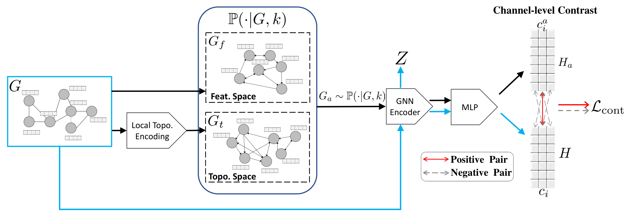
Refer to caption — Figure 1: Overview of FT-GCL. The input graph $G$ and its view $G_{a}$ are fed into the shared GNN encoder and MLP ( $G_{a}$ is FPG $G_{f}$ or TPG $G_{t}$ ). The final contrastive objective is to maximize the agreement of the distribution in the identical channels such as $c_{i}$ and $c^{a}_{i}$ , and distinguish different channels.

Step-1: Views generation

In this stage, we generate FPG and TPG of $G$ as two views to reflect proximity in the latent space. Figure 3 shows an example where nodes $u$ and $v$ have similar local topology: they have degrees 5 and 6, and are both connected to 2 triangles, therefore they should be connected in the topology space. To that end, we first encode the structural roles of each node as a vector in topology space. Although several structural role embedding methods [33, 13, 23] can do the job, they require separate back-propagation or enumeration operations, which are too heavy as a preprocessing step. Here, we provide an alternative method based on graph kernel.

We first extract local subgraphs for all the nodes, where the subgraphs can be $r$ -hop egonets (i.e., the induced subgraph surrounding each node) or induced by a set of random walk (RW) sequences start from each node. In effect, different choices do not affect the results significantly and RW is more efficient for dense graphs. Let $\mathcal{S}=\{S_{1},S_{2},\cdots,S_{N}\}$ be the set of extracted local subgraphs for each node, we adopt the Weisfeiler-Lehman (WL) subtree kernel [34] with a fixed number of iterations on the subgraph set $\mathcal{S}$ . Finally, we can obtain a symmetric positive semi-definite kernel matrix $K\in\mathbb{R}^{N\times N}$ , where $K_{ij}$ denotes the similarity between local subgraphs $S_{i}$ and $S_{j}$ , which can be seen as the local topological similarity between $v_{i}$ and $v_{j}$ . Then, we directly factorize $K$ to obtain the representation of each subgraph. This leads to a high computational complexity of $\mathcal{O}(N^{3})$ . We use Nyström approximation [46, 24] to reduce the cost to $\mathcal{O}(m^{2}N)$ , where $m\ll N$ . The Nyström method only uses a small subset of $m$ columns (or rows) of the $K$ , such that $K\approx RR^{\top}$ where $R\in\mathbb{R}^{N\times m}$ . Finally, each row of $R$ represents the coordinate of the corresponding node in the graph’s topology space, and therefore serves as the local topology representation of the node.

Figure 3 shows an experiment on a barbell graph $B(6,2)$ , where the local subgraphs are nodes’ 1-hop egonets. Based on $R$ , we construct a directed $k$ NN graph where each node links to top $k_{t}$ similar nodes using outgoing edges, denoted $G_{t}=(A_{t},\mathbf{X})$ . Note that in the views, $R$ is only used to generate the structure of $G_{t}$ and node features are still $\mathbf{X}$ .

In the feature space, a proximity graph $G_{f}$ is generated from $G$ based on node features $\mathbf{X}$ . Both proximity graphs use cosine similarity as the distance metric. In the views generation stage, the computational cost mainly comes from calculating the vector similarity for the $k$ NN graphs, which is $\mathcal{O}((F+m)N^{2})$ . Fortunately, fast approximiation [3, 54] and parallelization [5] methods have been well studied to construct $k$ NN graphs efficiently. For example, we are able to construct $k$ NN graphs with local sensitive hashing [54] in $\mathcal{O}(\ln(\max\{F,m\}+\log N))$ .

Two graph views $G_{f}$ and $G_{t}$ with $k_{f}=k_{t}=k$ are denoted $\mathbb{P}(\cdot|G,k)$ . In each training step, we randomly set a $k$ value and generate a view $G_{a}\sim\mathbb{P}(\cdot|G,k)$ , where $G_{a}$ is alternately set to $G_{f}$ or $G_{t}$ . The randomness of $k$ helps improve the view diversity, such that proximity with different scales can be preserved. However, repeatedly constructing $k$ NN graphs in each training step is expensive. We limit the values of $k_{f}$ and $k_{t}$ to $k_{max}$ , i.e., $k_{f},k_{t}\leq k_{max}$ . We only need to find top- $k_{max}$ neighbors for each node in the feature and the topology spaces before training, which is a single-time effort. Then in each training step, FPG with $k_{f}$ or TPG with $k_{t}$ can be easily obtained from the preprocessed $k_{max}$ neighbors by masking a certain number of neighbors at the end of the similarity ranking. In practice, $k_{max}$ is set manually as a hyperparameter and $k_{max}<10$ is found to work well.

Step-2: Shared GNN encoder

The view $G_{a}\sim\mathbb{P}(\cdot|G,k)$ together with $G$ are fed into a (Di)GNN encoder $\mathrm{GNN}(A,X)$ , where each node aggregates the messages propagated from its in-neighbors. The design of the GNN encoder is flexible. We find that GAT [41] or GraphSAGE [10] both perform well. The trainable parameter matrix $W^{(l)}$ in each layer is shared between two graphs during training.

Step-3: Shared MLP

After the GNN encoder, we use a shared Multi-Layer Perceptron (MLP) $g(\cdot)$ as a projection head [4, 52, 11] to enhance the expressive power of the output representations.

Step-4: Channel-level contrastive objective

The shared MLP outputs two representation matrices $H,H_{a}\in\mathbb{R}^{N\times d}$ for $G$ and its sampled augmented view $G_{a}$ , which can be seen as two signals with $d$ channels on two graph views. Different from previous work [57, 56, 16] that focuses on node-level contrasting, which suffers from high computation cost, we offer an alternative method that generates contrastive pairs at the channel level. Specifically, as shown in Figure 1 the $i$ -th channels of two output signals, denoted $c_{i}$ and $c^{a}_{i}$ , are the $i$ -th columns of $H$ and $H_{a}$ , respectively. Then the contrastive objective aims to maximize the consistency between two representation matrices, such that the distributions of identical channels $c_{i}$ and $c^{a}_{i}$ as inter-graph positive pairs are to be pulled together, and different channels $c_{i}$ and $c^{a}_{j,j\neq i}$ as negative pairs to be pushed away. Hence, the loss function of pair-wise channels $(c_{i},c^{a}_{i})$ is defined as:

\ell_{i}=-\left(\log\frac{\exp(\phi(c_{i},c^{a}_{i})/\tau)}{\sum_{j=1,j\neq i}^{d}\exp(\phi(c_{i},c^{a}_{j})/\tau)}+\log\frac{\exp(\phi(c_{i},c^{a}_{i})/\tau)}{\sum_{j=1,j\neq i}^{d}\exp(\phi(c_{j},c^{a}_{i})/\tau)}\right)

(2)

where $\tau$ is the temperature hyper-parameter to scale the cosine similarity $\phi(\cdot,\cdot)=\frac{\cdot^{\top}\cdot}{\lVert\cdot\rVert\lVert\cdot\rVert}$ . Chen et al. 2020 find that an appropriate $\tau$ can help the model learn from hard negatives. Considering all $d$ channels, the total contrastive loss function is as follows,

\mathcal{L}_{cont}=\frac{1}{d}\sum_{i}^{d}\ell_{i}

(3)

Prediction

The GNN encoder and MLP are all trained in an unsupervised manner. After the training stage, the original graph $G$ is fed into the GNN encoder to generate the resulting node embeddings $Z$ , as shown in the Figure 1. Then we can apply $Z$ to downstream prediction tasks such as node classification or link prediction. See appendix A for the summarized algorithm.

4.1 Theoretical Analysis

We create two graphs $G_{f}$ and $G_{t}$ as two views of $G$ , and then maximize the agreement between the output embedding matrices of $G$ and a view. By this means, the GNN encoder is able to capture richer semantic information (i.e., feature similarity and structural equivalence), which may boost the subsequent prediction tasks. In other words, minimizing the contrastive objective in Eq. (3) aims to maximize the “correlation” between the input graph $G$ and its proximity graph $G_{f}$ or $G_{t}$ . However, what does “correlation” specifically mean? In the following, we theoretically discuss the connection between the loss function of FT-GCL and InfoNCE [25] in detail to answer this question, and prove that minimizing our proposed channel-level contrastive objective can be viewed as a kind of maximizing a lower bound of the Mutual Information (MI) between $G$ and its views.

Given two view sets $A$ and $B$ , both with the same cardinality $n$ , there exists a bijection $\pi:A\to B$ such that each view of one set is positively paired with exactly one view of the other set. Any other inter-set pairs are negative. Under this condition, InfoNCE [25, 20] which is upper bounded by MI, can be defined as:

I_{NCE}(A;B)=\mathbb{E}_{(a,b)\sim\mathbb{P}(A,B)}\left[f_{\bm{\theta}}(a,b)-\log\mathbb{E}_{\widetilde{b}\sim\mathbb{P}(B)}\exp f_{\bm{\theta}}(a,\widetilde{b})\right]\leq I(A,B)

(4)

where $f_{\theta}(\cdot)\in\mathbb{R}$ is a function parameterized by $\theta$ , $\mathbb{P}(A,B)$ is the distribution of positive pairs. Then our contrastive objective Eq. (3) can be rewritten as the expectation form:

	$\displaystyle-\mathcal{L}_{cont}=$	$\displaystyle 2\mathbb{E}_{\mathbb{P}(c_{i},c^{a}_{i})}\frac{\phi(c_{i},c^{a}_{i})}{\tau}-\mathbb{E}_{\mathbb{P}(c_{i})}\log\mathbb{E}_{\mathbb{P}(c^{a}_{j})}\exp(\phi(c_{i},c^{a}_{j})/\tau)$		(5)
		$\displaystyle-\mathbb{E}_{\mathbb{P}(c^{a}_{i})}\log\mathbb{E}_{\mathbb{P}(c_{j})}\exp(\phi(c_{j},c^{a}_{i})/\tau)-2\log d,$		(5)

where $c^{a}=g(\mathrm{GNN}(G_{a}))$ , dimension $d$ is a constant. $\mathbb{P}(c_{i},c^{a}_{i})$ is a discrete uniform distribution of size $d$ , so $\mathbb{P}(c_{i},c^{a}_{i})=\mathbb{P}(c^{a}_{i})=\mathbb{P}(c_{i})$ . Let $f_{\theta}(c^{a},c^{b})=\phi(g(\mathrm{GNN}(G_{a})),g(\mathrm{GNN}(G_{b})))/\tau$ , where $\theta$ parametrized by $\tau$ and the MLP $g(\cdot)$ . Since there is bijection between column vector sets of $H$ and $H_{a}$ as positive pairs, then Eq. (5) can be transform to the InfoNCE form in Eq. (4) as:

	$\displaystyle-\mathcal{L}_{cont}=$	$\displaystyle 2\mathbb{E}_{\mathbb{P}(c_{i},c^{a}_{i})}f_{\theta}(c_{i},c^{a}_{i})-\mathbb{E}_{\mathbb{P}(c_{i})}\log\mathbb{E}_{\mathbb{P}(c^{a}_{j})}f_{\theta}(c_{i},c^{a}_{j})-$		(6)
		$\displaystyle\mathbb{E}_{\mathbb{P}(c^{a}_{i})}\log\mathbb{E}_{\mathbb{P}(c_{j})}f_{\theta}(c_{j},c^{a}_{i})\leq 2I(H,H_{a}),$		(6)

here we omit the constant $2\log d$ . The objective function of FT-GCL aims to maximize Eq. (6), that is equivalent to maximizing a lower bound of the mutual information between the output representation of $G$ and that of its proximity graph $G_{a}$ .

5 Experiments and Analysis

5.1 Effect of proximity graphs: ablation models

In FT-GCL, we do contrastive learning between the original graph and a sampled view in each training step, which raises a question: What is the effect of individual proximity graph on learning performance? To answer this question, we propose two ablation models: Feature proximity preserving GCL (F-GCL) and Topology proximity preserving GCL (T-GCL), as shown in Figure 4. In F-GCL, the original graph only contrasts with the feature proximity graph, while in T-GCL, the original graph only contrasts with the topology proximity graph. From these two models, we examine how feature proximity and topology proximity information benefit graph representation learning.

5.2 Node classification on assortative graphs

5.2.1 Experimentational setup

Datasets

We conduct experiments on the following seven real-world assortative graphs which are commonly used by existing work on graph learning. Table 1 summarizes the statistics of these benchmark datasets. See section B.1.1 for detailed description.

Evaluation protocol

For WikiCS, we directly use 20 public train/validation splits provided by Mernyei & Cangea 2020. For other datasets, we use ten splits of the nodes into 10%/10%/80% for train/validation/test nodes over 10 random seeds, then we run 10 times for each split to report average accuracy (Acc) and macro F1-score (Macro-F1). In the testing stage, the original graph is directly input into the GNN encoder and output a node representation matrix $Z\in\mathbb{R}^{N\times d^{\prime}}$ , as shown in Figure 1, then the embeddings of the training set are used to train a $l_{2}$ -regularized logistic regression classifier and give the results of classification on the test nodes. We provide implementation details in Section B.2, with hyper-parameters settings in Section B.3.

Table 1: Assortative datasets statistics.

	Cora	CiteSeer	PubMed	DBLP	WikiCS	BlogCatalog	ACM	CoauthorCS
$\|V\|$	2,708	3,327	19,717	17,716	11,701	5,196	3,025	18,333
$\|E\|$	5,429	4,732	44,338	52,867	216,123	171,743	13,128	81,894
$F$	1,433	3,703	500	1639	300	8,189	1,870	6,805
Classes	7	6	3	4	10	6	3	15

5.2.2 Baselines and results

We compare FT-GCL with two state-of-the-art unsupervised methods: (1) edge/path sampling based methods, including DeepWalk [31], node2vec [9] and LINE [38], and VERSE [39], (2) GNN based methods, including GAE/VGAE [18], ARVGA [26], MVGRL [11], DGI [42], GRACE [56], and GMI-Adaptive[30]. We also compare FT-GCL with several semi-supervised methods, including GCN [19], GAT [41], SGC [47] and JK-Net [49]. Limited by space, we report the results of Planetoid datasets in Table 2, which are the most commonly used benchmarks in the literature, and the results of other four datasets can be found in Appendix D.

Table 2: Average classification accuracy (%) and macro-F1 score (%) with standard deviation. The training data for each method is shown in Input column. For Planetoid datasets, we run 10 times over ten different random splits in order to comprehensively evaluate the generalization ability of the model on datasets. For clarity, and is the champion, is the runner-up.

	Input	Algo.	Cora		CiteSeer		PubMed
	Input	Algo.	Acc	Macro-F1	Acc	Macro-F1	Acc	Macro-F1
Unsupervised	$X$	Row features	$64.23(\pm 0.84)$	$60.14(\pm 1.25)$	$64.37(\pm 0.75)$	$60.05(\pm 1.57)$	$84.75(\pm 0.27)$	$84.67(\pm 0.24)$
	$A$	DeepWalk	$74.49(\pm 0.33)$	$73.06(\pm 0.20)$	$49.29(\pm 1.23)$	$46.86(\pm 1.52)$	$80.25(\pm 0.31)$	$78.82(\pm 0.33)$
		node2vec	$75.72(\pm 0.26)$	$74.15(\pm 0.17)$	$51.33(\pm 1.36)$	$47.37(\pm 1.60)$	$79.88(\pm 0.20)$	$78.34(\pm 0.24)$
		LINE	$56.33(\pm 0.20)$	$52.11(\pm 0.35)$	$34.74(\pm 0.85)$	$31.65(\pm 0.93)$	$69.31(\pm 0.13)$	$66.41(\pm 0.32)$
		VERSE	$75.87(\pm 0.70)$	$74.56(\pm 1.15)$	$53.37(\pm 1.05)$	$49.10(\pm 1.03)$	$80.45(\pm 0.24)$	$78.93(\pm 0.26)$
	$A$ , $X$	GAE	$81.37(\pm 1.06)$	$79.11(\pm 1.26)$	$68.42(\pm 0.56)$	$59.74(\pm 0.68)$	$80.81(\pm 0.35)$	$80.10(\pm 0.34)$
		VGAE	$80.80(\pm 1.30)$	$78.52(\pm 2.43)$	$69.60(\pm 0.55)$	$62.73(\pm 1.60)$	$82.25(\pm 0.28)$	$81.83(\pm 0.31)$
		ARVGA	$61.87(\pm 2.64)$	$56.05(\pm 4.91)$	$54.17(\pm 1.61)$	$46.32(\pm 1.77)$	$80.30(\pm 0.15)$	$79.79(\pm 0.17)$
		MVGRL	$83.77(\pm 0.67)$	$82.56(\pm 0.72)$	$\mathbf{73.35}(\pm 0.47)$	$\mathbf{66.89}(\pm 1.24)$	$85.33(\pm 0.16)$	$85.18(\pm 0.17)$
		DGI	$83.61(\pm 0.70)$	$82.27(\pm 0.85)$	$70.24(\pm 1.44)$	$65.60(\pm 0.97)$	$85.31(\pm 0.20)$	$84.74(\pm 0.20)$
		GRACE	$83.24(\pm 0.79)$	$81.26(\pm 0.51)$	$71.50(\pm 0.79)$	$64.99(\pm 1.78)$	$86.07(\pm 0.23)$	$84.79(\pm 0.22)$
		GMI-Adaptive	$83.51(\pm 0.66)$	$82.39(\pm 0.90)$	$72.18(\pm 0.35)$	$65.10(\pm 0.39)$	$82.97(\pm 1.01)$	$79.55(\pm 0.39)$
		F-GCL	$83.85(\pm 0.83)$	$81.85(\pm 1.04)$	$72.16(\pm 0.65)$	$66.44(\pm 0.80\textbf{})$	$86.15(\pm 0.33)$	$85.59(\pm 0.35)$
		T-GCL	$83.61(\pm 0.80)$	$82.65(\pm 0.92)$	$70.76(\pm 0.89)$	$65.49(\pm 1.12)$	$85.50(\pm 0.32)$	$84.94(\pm 0.33)$
		FT-GCL	$\mathbf{84.07}(\pm 0.58)$	$\mathbf{82.95}(\pm 0.79)$	$72.52(\pm 1.17)$	$66.79(\pm 1.74)$	$86.23(\pm 0.59)$	$85.31(\pm 0.28)$
Semi-supervised	$A$ , $X$ , $Y_{train}$	GCN	$82.57(\pm 0.22)$	$81.62(\pm 0.16)$	$71.81(\pm 0.65)$	$65.10(\pm 1.67)$	$\mathbf{86.36}(\pm 0.15)$	$\mathbf{85.77}(\pm 0.15)$
		GAT	$83.38(\pm 0.18)$	$82.09(\pm 0.36)$	$72.50(\pm 0.70)$	$65.23(\pm 0.97)$	$84.70(\pm 0.01)$	$84.03(\pm 0.38)$
		SGC	$80.28(\pm 0.20)$	$78.96(\pm 0.28)$	$71.97(\pm 0.01)$	$66.31(\pm 0.09)$	$81.35(\pm 0.19)$	$80.14(\pm 0.50)$
		JK-Net	$80.10(\pm 1.10)$	$79.73(\pm 0.81)$	$67.38(\pm 1.70)$	$61.95(\pm 0.20)$	$82.84(\pm 0.50)$	$78.33(\pm 0.02)$

As shown in Table 2, FT-GCL performs the best among unsupervised methods on Cora and PubMed. For the CiteSeer dataset, FT-GCL and MVGRL have comparable performance. Moreover, although without labels to guide the training, FT-GCL can also outperform the classical semi-supervised methods like GCN and GAT, and is only slightly weaker than GCN on PubMed. Note that MVGRL, DGI, GRACE, GMI, GRACE and our FT-GCL are contrastive learning (CL) based GNN models. Traditional network embedding methods like DeepWalk, node2vec and LINE can also be seen as a kind of CL-based method, where positive pairs are nodes with their contexts and negative pairs are nodes with their sampled negative nodes. However, these methods do not achieve desirable results. We think there are two reasons for this: first, node features are not involved in training; second, although they use negative sampling to accelerate the training process, the number of negative samples is usually very small.

The results of the two ablation models are also comparable with the state-of-the-art methods. For Cora, T-GCL achieves the second-best Macro-F1 score. For Pubmed, F-GCL achieves the second-best accuracy and the best Macro-F1 score among all unsupervised methods. The ablation study indicates that preserving either feature proximity or topology proximity during training can improve the quality of the representation vectors.

Figure 5: Comparing different graph augmentation schemes on GRACE.

Figure 6: Comparing node-level contrast with channel-level contrast on Cora(left) and CiteSeer(right).

\mathcal{L}_{FT-GCL}

and

\mathcal{L}_{FT-GCL-NL}

are loss values of FT-GCL and FT-GCL-NL, respectively.

Acc_{FT-GCL}

and

Acc_{FT-GCL-NL}

are their accuracy at several training epochs.

Given the results of all seven datasets in in Table 2 and Table 7, we consider that the strong performance of FT-GCL mainly comes from the idea of node proximity preserving. Compared with GRACE, FT-GCL is different in two respects: graph views generation and contrastive pair construction. Specifically, GRACE applies random corruption on the graph and node features to augment the graph, while FT-GCL uses two proximity graphs and do not modify the original features. In addition, GRACE builds contrastive pairs between two augmented graphs at an inter-graph and intra-graph node level, while FT-GCL only builds contrastive pairs between the original graph and one of the generated graph views at an inter-graph channel level.

We further replace the graph augmentation scheme of GRACE with proximity graphs as used in FT-GCL, called FT-GRACE. In addition, we replace the contrast scheme of FT-GCL with node-level contrast as used in GRACE, called FT-GCL-NL. Then, we compare the accuracy of GRACE and FT-GRACE to verify the proximity graphs’ adaptability, see Figure 6. The results on the three datasets show that proximity graphs also benefit other CL-based models and performs better than random corruption. Figure 6 shows that FT-GCL achieves better training performance than FT-GCL-NL, according to the speed of convergence. Besides, because FT-GCL-NL performs node-level contrast, the number of negative pairs is $O(N^{2})$ , where $N$ is the number of nodes. In FT-GCL, the number of negative pairs is reduced to $O(d^{2})$ , where $d$ is the number of channels of the output features. Usually, $d<<N$ , which means channel-level contrast is much more efficient than node-level contrast in large graphs.

5.3 Node classification on disassortative graphs

We also evaluate FT-GCL on a selection of disassortative graphs [29], namely Texas, Cornell, Wisconsin, and Actor. The statistics of datasets are shown in table 3, and more detailed descriptions are shown in section B.1.2. For all benchmarks, we use the same setting as [29] (10 public splits with 48%/32%20% of nodes per class for train/validation/test). Other parts of the evaluation protocol follow Section 5.2.1. Table 4 reports the average accuracy of our methods and other GNN-based models. We also consider a powerful variant of Gemo-GCN [29] which is shown to be powerful on disassortative graphs. The detailed analysis of this experiment is in Appendix C.

Table 3: Disassortative datasets statistics.

	Texas	Cornell	Wisconsin	Actor
$\|V\|$	183	183	251	7,600
$\|E\|$	295	280	466	26,752
$F$	1,703	1,703	1703	932
Classes	5	5	5	5

Table 4: Node classification accuracy (%) with standard deviation on disassortative graphs. is the champion, and is the runner-up.

	Algo.	Texas	Cornell	Wisconsin	Actor
Unsupervised	GAE	$56.22(\pm 4.32)$	$55.95(\pm 5.80)$	$47.25(\pm 6.35)$	$27.04(\pm 1.24)$
	VGAE	$54.86(\pm 6.17)$	$55.14(\pm 6.42)$	$48.63(\pm 5.46)$	$27.35(\pm 0.99)$
	ARVGA	$26.97(\pm 1.31)$	$57.57(\pm 4.99)$	$50.78(\pm 6.76)$	$25.27(\pm 1.16)$
	MVGRL	$63.84(\pm 4.09)$	$61.19(\pm 3.30)$	$64.12(\pm 7.44)$	$30.52(\pm 0.78)$
	DGI	$57.03(\pm 6.99)$	$55.68(\pm 4.86)$	$54.71(\pm 5.85)$	$26.80(\pm 0.88)$
	GRACE	$56.76(\pm 4.83)$	$53.78(\pm 7.20)$	$48.43(\pm 2.16)$	$27.06(\pm 1.19)$
	GMI-Adaptive	$53.24(\pm 7.74)$	$61.35(\pm 6.05)$	$53.92(\pm 7.19)$	$29.51(\pm 0.82)$
	F-GCL	$68.65(\pm 4.86)$	$68.46(\pm 7.55)$	$78.82(\pm 4.45)$	$36.26(\pm 0.78)$
	T-GCL	$72.70(\pm 4.59)$	$64.32(\pm 7.43)$	$75.29(\pm 4.57)$	$35.64(\pm 0.93)$
	FT-GCL	$71.35(\pm 5.30)$	$68.65(\pm 7.09)$	$75.88(\pm 4.02)$	$35.47(\pm 0.84)$
Semi-supervised	Geom-GCN-p	$67.57$	$60.81$	$64.12$	$31.63$
	GCN	$61.33(\pm 7.76)$	$56.78(\pm 4.58)$	$59.69(\pm 7.33)$	$30.28(\pm 0.69)$
	GAT	$58.93(\pm 4.37)$	$59.21(\pm 2.34)$	$53.03(\pm 8.37)$	$26.30(\pm 1.32)$
	JK-Net	$67.49(\pm 6.32)$	$67.93(\pm 7.46)$	$74.52(\pm 5.63)$	$35.10(\pm 0.85)$

5.4 Visiualization

We visualize the output embeddings learned by five unsupervised models using T-SNE [40]. High-quality embedding vectors exhibit low coupling and high cohesion. The results of Cora in Figure 7 are colored by real labels. From Figure 7, we find that although GAE and GRACE have relatively high cohesion, the intersection of multiple clusters is more chaotic. FT-GCL performs the best, where the learned representation vectors have higher intra-class similarity and more clear separation among different classes.

(a) DeepWalk

(b) GAE

(d) GRACE

(e) FT-GCL

Figure 7: T-SNE visualization of the output embeddings for the Cora dataset.

6 Conclusion

In this work, we propose FT-GCL, a self-supervised representation learning framework based on contrastive learning. FT-GCL aims to preserve multiple types of proximity information based on different definitions of node similarity. In FT-GCL, we propose proximity-based graph views based on feature similarity and local topology similarity, and then use a contrastive objective to maximize the agreement of the views and the original graph. In particular, we construct contrastive pairs on a channel level, by which we can greatly reduce the number of negative pairs. We show the connection between InfoNCE and the objective of FT-GCL, which justifies the rationality of our model. Experimental results on 11 datasets show that FT-GCL and its variants are all competitive against state-of-the-art methods.

Acknowledgments and Disclosure of Funding

References

Bojchevski & Günnemann [2018] Bojchevski, A. and Günnemann, S. Deep gaussian embedding of graphs: Unsupervised inductive learning via ranking. In International Conference on Learning Representations, 2018. URL https://openreview.net/forum?id=r1ZdKJ-0W.
Bruna & Li [2017] Bruna, J. and Li, X. Community detection with graph neural networks. stat, 1050:27, 2017.
Chen et al. [2009] Chen, J., Fang, H.-r., and Saad, Y. Fast approximate knn graph construction for high dimensional data via recursive lanczos bisection. Journal of Machine Learning Research, 10(9), 2009.
Chen et al. [2020] Chen, T., Kornblith, S., Norouzi, M., and Hinton, G. A simple framework for contrastive learning of visual representations. In International conference on machine learning, pp. 1597–1607. PMLR, 2020.
Dong et al. [2011] Dong, W., Moses, C., and Li, K. Efficient k-nearest neighbor graph construction for generic similarity measures. In Proceedings of the 20th international conference on World wide web, pp. 577–586, 2011.
Donnat et al. [2018] Donnat, C., Zitnik, M., Hallac, D., and Leskovec, J. Learning structural node embeddings via diffusion wavelets. In Proceedings of the 24th ACM SIGKDD International Conference on Knowledge Discovery & Data Mining, pp. 1320–1329, 2018.
Fey & Lenssen [2019] Fey, M. and Lenssen, J. E. Fast graph representation learning with pytorch geometric. arXiv preprint arXiv:1903.02428, 2019.
Gilmer et al. [2017] Gilmer, J., Schoenholz, S. S., Riley, P. F., Vinyals, O., and Dahl, G. E. Neural message passing for quantum chemistry. In International Conference on Machine Learning, pp. 1263–1272. PMLR, 2017.
Grover & Leskovec [2016] Grover, A. and Leskovec, J. node2vec: Scalable feature learning for networks. In Proceedings of the 22nd ACM SIGKDD international conference on Knowledge discovery and data mining, pp. 855–864, 2016.
Hamilton et al. [2017] Hamilton, W. L., Ying, R., and Leskovec, J. Inductive representation learning on large graphs. In NIPS, 2017.
Hassani & Khasahmadi [2020] Hassani, K. and Khasahmadi, A. H. Contrastive multi-view representation learning on graphs. In International Conference on Machine Learning, pp. 4116–4126. PMLR, 2020.
He et al. [2020] He, K., Fan, H., Wu, Y., Xie, S., and Girshick, R. Momentum contrast for unsupervised visual representation learning. In Proceedings of the IEEE/CVF Conference on Computer Vision and Pattern Recognition, pp. 9729–9738, 2020.
Henderson et al. [2012] Henderson, K., Gallagher, B., Eliassi-Rad, T., Tong, H., Basu, S., Akoglu, L., Koutra, D., Faloutsos, C., and Li, L. Rolx: structural role extraction & mining in large graphs. In Proceedings of the 18th ACM SIGKDD international conference on Knowledge discovery and data mining, pp. 1231–1239, 2012.
Hu et al. [2020] Hu, Z., Dong, Y., Wang, K., Chang, K.-W., and Sun, Y. Gpt-gnn: Generative pre-training of graph neural networks. In Proceedings of the 26th ACM SIGKDD International Conference on Knowledge Discovery & Data Mining, pp. 1857–1867, 2020.
Jin et al. [2021] Jin, W., Derr, T., Wang, Y., Ma, Y., Liu, Z., and Tang, J. Node similarity preserving graph convolutional networks. In Proceedings of the 14th ACM International Conference on Web Search and Data Mining, pp. 148–156, 2021.
Jovanović et al. [2021] Jovanović, N., Meng, Z., Faber, L., and Wattenhofer, R. Towards robust graph contrastive learning. arXiv preprint arXiv:2102.13085, 2021.
Kingma & Ba [2014] Kingma, D. P. and Ba, J. Adam: A method for stochastic optimization. arXiv preprint arXiv:1412.6980, 2014.
Kipf & Welling [2016] Kipf, T. N. and Welling, M. Variational graph auto-encoders. NIPS Workshop on Bayesian Deep Learning, 2016.
Kipf & Welling [2017] Kipf, T. N. and Welling, M. Semi-supervised classification with graph convolutional networks. In International Conference on Learning Representations (ICLR), 2017.
Kong et al. [2019] Kong, L., d’Autume, C. d. M., Ling, W., Yu, L., Dai, Z., and Yogatama, D. A mutual information maximization perspective of language representation learning. arXiv preprint arXiv:1910.08350, 2019.
Meng et al. [2019] Meng, Z., Liang, S., Bao, H., and Zhang, X. Co-embedding attributed networks. In Proceedings of the Twelfth ACM International Conference on Web Search and Data Mining, pp. 393–401, 2019.
Mernyei & Cangea [2020] Mernyei, P. and Cangea, C. Wiki-cs: A wikipedia-based benchmark for graph neural networks. arXiv preprint arXiv:2007.02901, 2020.
Narayanan et al. [2016] Narayanan, A., Chandramohan, M., Chen, L., Liu, Y., and Saminathan, S. subgraph2vec: Learning distributed representations of rooted sub-graphs from large graphs. arXiv preprint arXiv:1606.08928, 2016.
Nikolentzos et al. [2018] Nikolentzos, G., Meladianos, P., Tixier, A. J.-P., Skianis, K., and Vazirgiannis, M. Kernel graph convolutional neural networks. In International Conference on Artificial Neural Networks, pp. 22–32. Springer, 2018.
Oord et al. [2018] Oord, A. v. d., Li, Y., and Vinyals, O. Representation learning with contrastive predictive coding. arXiv preprint arXiv:1807.03748, 2018.
Pan et al. [2018] Pan, S., Hu, R., Long, G., Jiang, J., Yao, L., and Zhang, C. Adversarially regularized graph autoencoder for graph embedding. In IJCAI, pp. 2609–2615, 2018.
Park et al. [2019] Park, J., Lee, M., Chang, H. J., Lee, K., and Choi, J. Y. Symmetric graph convolutional autoencoder for unsupervised graph representation learning. In Proceedings of the IEEE/CVF International Conference on Computer Vision, pp. 6519–6528, 2019.
Pedregosa et al. [2011] Pedregosa, F., Varoquaux, G., Gramfort, A., Michel, V., Thirion, B., Grisel, O., Blondel, M., Prettenhofer, P., Weiss, R., Dubourg, V., et al. Scikit-learn: Machine learning in python. the Journal of machine Learning research, 12:2825–2830, 2011.
Pei et al. [2019] Pei, H., Wei, B., Chang, K. C.-C., Lei, Y., and Yang, B. Geom-gcn: Geometric graph convolutional networks. In International Conference on Learning Representations, 2019.
Peng et al. [2020] Peng, Z., Huang, W., Luo, M., Zheng, Q., Rong, Y., Xu, T., and Huang, J. Graph representation learning via graphical mutual information maximization. In Proceedings of The Web Conference 2020, pp. 259–270, 2020.
Perozzi et al. [2014] Perozzi, B., Al-Rfou, R., and Skiena, S. Deepwalk: Online learning of social representations. In Proceedings of the 20th ACM SIGKDD international conference on Knowledge discovery and data mining, pp. 701–710, 2014.
Qiu et al. [2020] Qiu, J., Chen, Q., Dong, Y., Zhang, J., Yang, H., Ding, M., Wang, K., and Tang, J. Gcc: Graph contrastive coding for graph neural network pre-training. In Proceedings of the 26th ACM SIGKDD International Conference on Knowledge Discovery & Data Mining, pp. 1150–1160, 2020.
Ribeiro et al. [2017] Ribeiro, L. F., Saverese, P. H., and Figueiredo, D. R. struc2vec: Learning node representations from structural identity. In Proceedings of the 23rd ACM SIGKDD international conference on knowledge discovery and data mining, pp. 385–394, 2017.
Shervashidze et al. [2011] Shervashidze, N., Schweitzer, P., Van Leeuwen, E. J., Mehlhorn, K., and Borgwardt, K. M. Weisfeiler-lehman graph kernels. Journal of Machine Learning Research, 12(9), 2011.
Shuman et al. [2013] Shuman, D. I., Narang, S. K., Frossard, P., Ortega, A., and Vandergheynst, P. The emerging field of signal processing on graphs: Extending high-dimensional data analysis to networks and other irregular domains. IEEE signal processing magazine, 30(3):83–98, 2013.
Sinha et al. [2015] Sinha, A., Shen, Z., Song, Y., Ma, H., Eide, D., Hsu, B.-J., and Wang, K. An overview of microsoft academic service (mas) and applications. In Proceedings of the 24th international conference on world wide web, pp. 243–246, 2015.
Sun et al. [2019] Sun, F.-Y., Hoffman, J., Verma, V., and Tang, J. Infograph: Unsupervised and semi-supervised graph-level representation learning via mutual information maximization. In International Conference on Learning Representations, 2019.
Tang et al. [2015] Tang, J., Qu, M., Wang, M., Zhang, M., Yan, J., and Mei, Q. Line: Large-scale information network embedding. In Proceedings of the 24th international conference on world wide web, pp. 1067–1077, 2015.
Tsitsulin et al. [2018] Tsitsulin, A., Mottin, D., Karras, P., and Müller, E. Verse: Versatile graph embeddings from similarity measures. In Proceedings of the 2018 world wide web conference, pp. 539–548, 2018.
Van der Maaten & Hinton [2008] Van der Maaten, L. and Hinton, G. Visualizing data using t-sne. Journal of machine learning research, 9(11), 2008.
Veličković et al. [2018] Veličković, P., Cucurull, G., Casanova, A., Romero, A., Liò, P., and Bengio, Y. Graph Attention Networks. International Conference on Learning Representations, 2018. URL https://openreview.net/forum?id=rJXMpikCZ. accepted as poster.
Veličković et al. [2019] Veličković, P., Fedus, W., Hamilton, W. L., Liò, P., Bengio, Y., and Hjelm, R. D. Deep Graph Infomax. In International Conference on Learning Representations, 2019. URL https://openreview.net/forum?id=rklz9iAcKQ.
Wang et al. [2017] Wang, X., Cui, P., Wang, J., Pei, J., Zhu, W., and Yang, S. Community preserving network embedding. In Proceedings of the AAAI Conference on Artificial Intelligence, volume 31, 2017.
Wang et al. [2019] Wang, X., Ji, H., Shi, C., Wang, B., Ye, Y., Cui, P., and Yu, P. S. Heterogeneous graph attention network. In The World Wide Web Conference, pp. 2022–2032, 2019.
Wang et al. [2020] Wang, X., Zhu, M., Bo, D., Cui, P., Shi, C., and Pei, J. Am-gcn: Adaptive multi-channel graph convolutional networks. In Proceedings of the 26th ACM SIGKDD International Conference on Knowledge Discovery & Data Mining, pp. 1243–1253, 2020.
Williams & Seeger [2001] Williams, C. and Seeger, M. Using the nyström method to speed up kernel machines. In Proceedings of the 14th annual conference on neural information processing systems, number CONF, pp. 682–688, 2001.
Wu et al. [2019] Wu, F., Souza, A., Zhang, T., Fifty, C., Yu, T., and Weinberger, K. Simplifying graph convolutional networks. In International conference on machine learning, pp. 6861–6871. PMLR, 2019.
Wu et al. [2018] Wu, Z., Xiong, Y., Yu, S. X., and Lin, D. Unsupervised feature learning via non-parametric instance discrimination. In Proceedings of the IEEE Conference on Computer Vision and Pattern Recognition, pp. 3733–3742, 2018.
Xu et al. [2018] Xu, K., Li, C., Tian, Y., Sonobe, T., Kawarabayashi, K.-i., and Jegelka, S. Representation learning on graphs with jumping knowledge networks. In International Conference on Machine Learning, pp. 5453–5462. PMLR, 2018.
Yang et al. [2016] Yang, Z., Cohen, W., and Salakhudinov, R. Revisiting semi-supervised learning with graph embeddings. In International conference on machine learning, pp. 40–48. PMLR, 2016.
Ying et al. [2018] Ying, Z., You, J., Morris, C., Ren, X., Hamilton, W. L., and Leskovec, J. Hierarchical graph representation learning with differentiable pooling. In NeurIPS, 2018.
You et al. [2020] You, Y., Chen, T., Sui, Y., Chen, T., Wang, Z., and Shen, Y. Graph contrastive learning with augmentations. Advances in Neural Information Processing Systems, 33, 2020.
Zhang & Chen [2018] Zhang, M. and Chen, Y. Link prediction based on graph neural networks. In NeurIPS, 2018.
Zhang et al. [2013] Zhang, Y.-M., Huang, K., Geng, G., and Liu, C.-L. Fast knn graph construction with locality sensitive hashing. In Joint European Conference on Machine Learning and Knowledge Discovery in Databases, pp. 660–674. Springer, 2013.
Zhu et al. [2020a] Zhu, J., Yan, Y., Zhao, L., Heimann, M., Akoglu, L., and Koutra, D. Beyond homophily in graph neural networks: Current limitations and effective designs. Advances in Neural Information Processing Systems, 33, 2020a.
Zhu et al. [2020b] Zhu, Y., Xu, Y., Yu, F., Liu, Q., Wu, S., and Wang, L. Deep graph contrastive representation learning. arXiv preprint arXiv:2006.04131, 2020b.
Zhu et al. [2020c] Zhu, Y., Xu, Y., Yu, F., Liu, Q., Wu, S., and Wang, L. Graph contrastive learning with adaptive augmentation. arXiv preprint arXiv:2010.14945, 2020c.

Appendix A Feature and topology proximity graph generation algorithms

Algorithm 1 TPG Generation

1: Input: Graph

G=(V,E,\mathbf{X})

; WL kernel

k

with

t

iterations; Number of neighbors

k_{t}

; Number of walks

\gamma

, Walk length

l

; Number of basis vectors

m

2: Output: Topology proximity graph

G_{t}=(A_{t},\mathbf{X})

3: for each

v_{i}\in V

\mathcal{S}_{i}\leftarrow\mathrm{Subgraph}(\mathrm{RW}(v_{i},l,\gamma))

\triangleright

Subgraph induced by random walk node sequences

5: end for

\widetilde{\mathcal{S}}\sim\mathbb{P}(\mathcal{S})

\triangleright

Random sample

m

subgraphs as basis,

|\widetilde{\mathcal{S}}|=m

\mathcal{K}\leftarrow k(\mathcal{S},\widetilde{\mathcal{S}})

\triangleright

Compute kernel matrix between

\mathcal{S}

and

\widetilde{\mathcal{S}}

, where

\mathcal{K}\in\mathbb{R}^{N\times m}

\widetilde{\mathcal{K}}\leftarrow k(\widetilde{\mathcal{S}},\widetilde{\mathcal{S}})

\triangleright

Comput kernel matrix among basis subgraphs, where

\widetilde{\mathcal{K}}\in\mathbb{R}^{m\times m}

U,S,V^{\prime}=\mathrm{SVD}(\widetilde{\mathcal{K}})

10:

\widehat{\mathcal{K}}\leftarrow US^{-\frac{1}{2}}V^{\prime}

\triangleright

Normalize

\widetilde{\mathcal{K}}

11:

R\leftarrow\mathcal{K}\widehat{\mathcal{K}}

\triangleright

Local topology representation, where

R\in\mathbb{R}^{N\times m}

12:

A_{t}\leftarrow k\mathrm{NN}(R,k_{t})

\triangleright

Contrust

k

NN graph based on

R

13: return

G_{t}=(A_{t},\mathbf{X})

Algorithm 2 FT-GCL

1: Input: Graph

G=(V,E,\mathbf{X})

; Upper limit of the number of neighbors

k_{max}

; Pre-generated structural embedding

R

; Number of iterations

T

; Temperature hyper-parameter

\tau

; Hidden and output dimension of the projection head

d

; Hidden dimension and output dimension of the GNN encoder

d^{\prime}

\widehat{A}_{f}\leftarrow k\mathrm{NN}(\mathbf{X},k_{max})

\triangleright

Generate

G_{f}=(\widehat{A}_{f},\mathbf{X})

based on

\mathbf{X}

\widehat{A}_{t}\leftarrow k\mathrm{NN}(R,k_{max})

\triangleright

Generate

G_{t}=(\widehat{A}_{t},\mathbf{X})

based on

R

\mathrm{Use\_FPG}\leftarrow\mathrm{True}

5: for

t=1,2,\cdots,T

6: Random sample

k\leq k_{max}

7: if

\mathrm{Use\_FPG}

is True then

A_{f}=\mathrm{Mask}(\widehat{A}_{f},k_{max}-k)

\triangleright

Mask the

k_{max}-k

least similar neighbors for each node

G_{f}=(A_{f},\mathbf{X})

10:

G_{a}\leftarrow G_{f}

11: else

12:

A_{t}=\mathrm{Mask}(\widehat{A}_{t},k_{max}-k)

13:

G_{t}=(A_{t},\mathbf{X})

14:

G_{a}\leftarrow G_{t}

15: end if

16:

Z\leftarrow\mathrm{GNN}(G)

Z_{a}\leftarrow\mathrm{GNN}(G_{a})

\triangleright

The shared GNN encoder,

Z,Z_{a}\in\mathbb{R}^{N\times d^{\prime}}

17:

H\leftarrow g(Z)

H_{a}\leftarrow g(Z_{a})

\triangleright

The projection head,

H,H_{a}\in\mathbb{R}^{N\times d}

18:

\mathcal{L}\leftarrow Eq.(\ref{eq:total_cl})

\triangleright

Channel-level contrastive loss

19: if

\mathrm{Use\_FPG}

is True then

20:

\mathrm{Use\_FPG}\leftarrow\mathrm{False}

21: else

22:

\mathrm{Use\_FPG}\leftarrow\mathrm{True}

23: end if

24: end for

Appendix B Reproducibility

B.1 Datasets details

B.1.1 Assortative datasets

The Planetoid [50] datasets (i.e., Cora, CiteSeer, and PubMed) and DBLP [1] are citation networks, where nodes represent documents and edges citation links. WikiCS [22] is a Wikipedia-based dataset, which consists of nodes corresponding to Computer Science articles, and edges based on hyperlinks, as well as 10 classes representing different branches of the field. BlogCatalog [21] is a social network with bloggers and their social relationships from the BlogCatalog website, where node features are constructed by the keywords of user profiles. ACM [44] and CoauthorCS [36] are coauthor networks, where edges’ endpoints are two papers with the same authors.

B.1.2 Disassortative datasets

Texas, Wisconsin and Cornell are graphs where nodes are web pages of the corresponding universities and edges are links between web pages. Node features are the bag-of-words representation of web pages. These graphs are originally collected by the CMU WebKB project. Actor is a co-occurence network where each node correspond to an actor, and the edge between two nodes denotes co-occurrence on the same Wikipedia page. Node features correspond to some keywords in the Wikipedia pages. We used the preprocessed version of these four datasets in [29].

B.2 Implementation Details

In the graph view generation stage, for topology proximity graph $G_{t}$ the local subgraph of each node is induced by $\gamma$ random walk sequences of length $l$ . We use alias sampling such that the sampling complexity is $\mathcal{O}(\gamma lN)$ . We set $\gamma=30$ , $l=10$ for all benchmark graphs. We use the WL kernel with the Nyström method to encode local topology for each node, and the number of basis vectors $m$ is set to $200$ for all graphs. For the shared GNN encoder, we use 2-layers Graph Attention Networks [41] with a single head by default. FT-GCL does not impose any constraint on the GNN architecture, so other GNNs such as GraphSAGE can be also used. The activation function $\sigma$ of the GNN encoder is selected from $\{\mathrm{ReLU},\mathrm{eLU},\mathrm{PReLU}\}$ . We use Adam [17] for optimizing $\mathcal{L}_{cont}$ with learning rate $lr$ from $\{1e^{-2},1e^{-3},5e^{-3},5e^{-4}\}$ . The hidden layer and the output layer of the GNN encoder have the same number of dimensions $d^{\prime}$ , which is selected from $\{64,128,256,512\}$ . The hidden layer and the output layer of the MLP have the same number of dimensions $d$ , which is also selected from $\{64,128,256,512\}$ . The value of weight decay is selected from $\lambda\in\{1e^{-4},5e^{-3},5e^{-4}.5e^{-5}\}$ The experiments are implemented using Pytorch Geometric 1.6.1 [7] with CUDA version 10.2, networkx 2.5, Python 3.8.5, scikit-learn [28] 0.23.2. The experiments are conducted on Linux servers installed with a NVIDIA Quadro RTX8000 GPU and 10 Intel(R) Xeon(R) Silver 4210R CPUs.

B.3 Hyperparameter Specifications

Table 5: Hyperparameter for FT-GCL on all benchmarks.

Benchmarks	$k_{max}$	$d$	$d^{\prime}$	$lr$	$\tau$	$\lambda$	$\sigma$
Cora	8	512	256	$5e^{-4}$	0.2	$5e^{-5}$	PReLU
CiteSeer	5	512	64	$5e^{-4}$	0.2	$5e^{-3}$	eLU
PubMed	10	512	128	$5e^{-3}$	0.9	$5e^{-4}$	eLU
DBLP	10	512	64	$5e^{-4}$	0.4	$5e^{-5}$	PReLU
WikiCS	10	256	128	$5e^{-4}$	0.2	$5e^{-4}$	eLU
ACM	10	512	64	$1e^{-3}$	0.7	$5e^{-4}$	ReLU
CoauthorCS	10	512	512	$5e^{-4}$	0.1	$1e^{-4}$	eLU
Texas	10	64	128	$1e^{-3}$	0.2	$5e^{-4}$	ReLU
Wisconsin	10	64	128	$1e^{-3}$	0.2	$5e^{-4}$	ReLU
Cornell	10	128	128	$1e^{-3}$	0.2	$5e^{-4}$	ReLU
Actor	10	128	64	$1e^{-2}$	0.2	$5e^{-5}$	ReLU

Appendix C Analysis of Section 5.3

The results of node classification task on disassortative graphs in Table 4 show that FT-GCL and its two variants F-GCL and T-GCL outperform other models with a significant margin. In this section, we give an analysis based on the edge homophily ratio (EHR) defined in Zhu et al. 2020a:

h=\frac{\left|\left\{(v_{i},v_{j}):(v_{i},v_{j})\in E\wedge y_{i}=y_{j}\right\}\right|}{|E|},

(7)

which means the proportion of the intra-class edges to the total number of edges. It can be used as a measure of the graph’s homophily level. For all disassortative benchmarks, we report the EHR values on the original graph $G$ , its FPG $G_{f}$ and TPG $G_{t}$ in Table 6. We find that all the four datasets have weak homophily. However, both the FPG and TPG of Texas and Cornell have strong homophily, i.e., $h_{f},h_{t}>0.5$ . This explains why F-GCL, T-GCL and FT-GCL outperform other methods. Since Wisconsin’s FPG has strong homophily, F-GCL and FT-GCL achieve the best results. It is worth noting that although the two proximity graphs of Actor have weak homophily, exploiting multiple types of proximity can also help our model learn relatively better embeddings. The experiments in Section 5.3 suggest that FPG and TPG are complementary to the original graph, which is particularly evident in the disassortative graphs with low homophily.

Table 6: The edge homophily ratio of

G

G_{f}

and

G_{t}

(

k_{f}=k_{s}=6

) on four disassortative graphs.

	Texas	Wisconsin	Cornell	Actor
Homo. ratio $h$	0.108	0.196	0.305	0.219
FPG Homophily ratio $h_{f}$	0.657	0.699	0.657	0.250
TPG Homophily ratio $h_{t}$	0.530	0.337	0.530	0.233

Appendix D More experiments

D.1 Node classification

In this section, we show the results of node classification for the DBLP, WikiCS, BlogCatalog, ACM and CoathorCS datasets in Table 7. Among these four additional experiments, the previous state-of-the-art GRACE and MVGRL achieve the best results on DBLP and BlogCatalog, respectively. Our proposed FT-GCL performs the best on WikiCS and ACM, and achieves the second-best results on CoauthorCS among all unsupervised methods. In addition, F-GCL achieves the second-best results on DBLP, WikiCS and ACM, and is the best unsupervised method on CoauthorCS.

Table 7: Classification accuracies(%) and macro-F1 scores(%) with standard deviation. is the champion and is the runner-up.

	Input	Algo.	DBLP		WikiCS		ACM		CoauthorCS
	Input	Algo.	Acc	Macro-F1	Acc	Macro-F1	Acc	Macro-F1	Acc	Macro-F1
Unsupervised	$X$	Row features	$71.22(\pm 0.71)$	$64.62(\pm 0.76)$	$72.67(\pm 0.62)$	$69.24(\pm 0.82)$	$86.40(\pm 0.42)$	$86.40(\pm 0.41)$	$90.18(\pm 0.07)$	$87.21(\pm 0.14)$
	$A$	DeepWalk	$78.92(\pm 0.20)$	$72.71(\pm 0.80)$	$68.33(\pm 1.27)$	$64.64(\pm 1.39)$	$60.09(\pm 0.16)$	$55.32(\pm 1.71)$	$85.00(\pm 0.38)$	$83.58(\pm 0.29)$
		node2vec	$79.45(\pm 0.24)$	$73.11(\pm 0.36)$	$69.06(\pm 0.75)$	$65.19(\pm 0.80)$	$61.15(\pm 0.77)$	$57.28(\pm 0.09)$	$84.97(\pm 0.36)$	$83.29(\pm 0.62)$
		LINE	$64.03(\pm 0.33)$	$56.45(\pm 0.70)$	$67.36(\pm 0.89)$	$63.84(\pm 0.96)$	$41.33(\pm 0.57)$	$39.90(\pm 0.25)$	$77.45(\pm 0.40)$	$69.95(\pm 1.23)$
		VERSE	$79.22(\pm 0.33)$	$73.07(\pm 0.58)$	$72.67(\pm 0.62)$	$69.24(\pm 0.82)$	$69.18(\pm 0.83)$	$69.16(\pm 0.83)$	$86.56(\pm 0.30)$	$82.75(\pm\textbf{{}}0.68)$
	$A$ , $X$	GAE	$82.36(\pm 0.18)$	$78.91(\pm 0.39)$	$68.72(\pm 0.52)$	$60.84(\pm 0.90)$	$87.62(\pm 0.66)$	$87.51(\pm 0.65)$	$92.46(\pm 0.20)$	$90.09(\pm 0.44)$
		VGAE	$82.68(\pm 0.22)$	$79.45(\pm 0.34)$	$75.64(\pm 0.63)$	$71.83(\pm 0.84)$	$89.78(\pm 0.48)$	$89.73(\pm 0.47)$	$92.10(\pm 0.22)$	$89.85(\pm 0.46)$
		ARVGA	$75.77(\pm 0.43)$	$66.83(\pm 0.85)$	$67.35(\pm 0.49)$	$60.75(\pm 0.83)$	$74.07(\pm 1.31)$	$74.37(\pm 1.48)$	$88.54(\pm 0.23)$	$83.76(\pm 0.38)$
		MVGRL	$83.68(\pm 0.17)$	$79.54(\pm 0.24)$	$74.13(\pm 0.64)$	$68.89(\pm 1.42)$	$90.80(\pm 0.31)$	$90.81(\pm 0.32)$	$92.08(\pm 0.50)$	$90.93(\pm 0.42)$
		DGI	$83.11(\pm 0.19)$	$78.64(\pm 0.44)$	$75.70(\pm 0.45)$	$72.12(\pm 0.69)$	$90.01(\pm 0.30)$	$90.00(\pm 0.33)$	$92.30(\pm 0.16)$	$90.45(\pm 0.32)$
		GRACE	$\mathbf{84.45}(\pm 0.19)$	$\mathbf{80.31}(\pm 0.26)$	$78.26(\pm 0.15)$	$75.96(\pm 0.71)$	$90.28(\pm 0.46)$	$90.27(\pm 0.48)$	$92.42(\pm 0.20)$	$90.44(\pm 0.25)$
		GMI-Adaptive	$83.51(\pm 0.32)$	$78.66(\pm 0.40)$	$77.57(\pm 0.44)$	$74.65(\pm 0.63)$	$87.15(\pm 0.53)$	$87.17(\pm 0.53)$	$91.92(\pm 0.13)$	$89.06(\pm 0.31)$
		F-GCL	$83.85(\pm 0.15)$	$79.74(\pm 0.21)$	$78.69(\pm 0.66)$	$75.38(\pm 0.70)$	$90.99(\pm 0.15)$	$91.01(\pm 0.15)$	$\mathbf{93.06}(\pm 0.15)$	$91.04(\pm 0.20)$
		T-GCL	$82.79(\pm 0.35)$	$78.43(\pm 0.55)$	$76.74(\pm 0.23)$	$72.81(\pm 0.15)$	$87.39(\pm 0.33)$	$87.44(\pm 0.33)$	$92.77(\pm 0.04)$	$90.74(\pm 0.27)$
		FT-GCL	$83.58(\pm 0.64)$	$79.52(\pm 0.39)$	$\mathbf{78.91}(\pm 0.61)$	$\mathbf{76.53}(\pm 0.38)$	$\mathbf{91.28}(\pm 0.18)$	$\mathbf{91.28}(\pm 0.19)$	$92.94(\pm 0.03)$	$90.81(\pm 0.27)$
Semi-supervised	$A$ , $X$ , $Y_{train}$	GCN	$82.73(\pm 0.58)$	$77.34(\pm 0.29)$	$76.40(\pm 1.00)$	$72.35(\pm 0.21)$	$87.66(\pm 1.18)$	$87.76(\pm 1.51)$	$93.05(\pm 0.26)$	$\mathbf{91.07}(\pm 0.22)$
		GAT	$83.39(\pm 0.16)$	$79.11(\pm 0.10)$	$77.60(\pm 0.60)$	$74.37(\pm 0.88)$	$86.52(\pm 0.97)$	$86.75(\pm 1.08)$	$92.42(\pm 0.29)$	$90.38(\pm 0.10)$
		SGC	$82.10(\pm 0.12)$	$76.99(\pm 0.56)$	$74.92(\pm 0.22)$	$71.66(\pm 0.23)$	$88.65(\pm 0.37)$	$88.77(\pm 0.26)$	$93.10(\pm 0.78)$	$90.88(\pm 0.30)$
		JK-Net	$81.82(\pm 0.80)$	$77.54(\pm 0.35)$	$68.93(\pm 0.89)$	$66.75(\pm 0.62)$	$88.20(\pm 0.80)$	$88.23(\pm 0.16)$	$89.60(\pm 0.22)$	$85.96(\pm 0.10)$

We also conduct experiments on public splits of Planetoid datasets provided by [50], and report the results in Table 8.

Table 8: Averaged classification accuracies(%) with standard deviation on Planetoid datasets (public splits). is the champion and is the runner-up.

	Input	Algo.	Cora	CiteSeer	PubMed
	$A$ , $X$	GAE	$71.5(\pm 0.4)$	$65.8(\pm 0.4)$	$72.1(\pm 0.5)$
Unsupervised		VGAE	$75.2(\pm 0.2)$	$69.0(\pm 0.2)$	$75.3(\pm 0.5)$
		ARVGA	$74.4(\pm 0.1)$	$64.2(\pm 0.6)$	$74.7(\pm 0.7)$
		MVGRL	$82.9(\pm 0.7)$	$72.6(\pm 0.7)$	$79.4(\pm 0.3)$
		DGI	$82.3(\pm 0.6)$	$71.8(\pm 0.7)$	$76.8(\pm 0.6)$
		GRACE	$80.0(\pm 0.4)$	$71.7(\pm 0.6)$	$79.5(\pm 1.1)$
		GMI-Adaptive	$83.0(\pm 0.3)$	$72.4(\pm 0.1)$	$\mathbf{79.9}(\pm 0.2)$
		F-GCL	$82.9(\pm 0.5)$	$72.2(\pm 0.4)$	$\mathbf{79.9}(\pm 0.3)$
		T-GCL	$80.8(\pm 0.1)$	$\mathbf{73.3}(\pm 0.2)$	$77.7(\pm 0.7)$
		FT-GCL	$\mathbf{83.1}(\pm 0.3)$	$72.6(\pm 0.3)$	$79.8(\pm 0.6)$
Semi-supervised	$A$ , $X$ , $Y_{train}$	GCN	$81.5(\pm 0.4)$	$70.3(\pm 0.7)$	$79.0(\pm 0.5)$
		GAT	$83.0(\pm 0.7)$	$72.5(\pm 0.7)$	$79.0(\pm 0.3)$
		SGC	$81.0(\pm 0.0)$	$71.9(\pm 0.1)$	$78.9(\pm 0.0)$

D.2 Link Prediction

In this section, we evaluate the performance on the link prediction task. We conduct experiments on Cora and CiteSeer, removing 5% existing edges and the same-size non-existing edges for validation, 10% existing edges and the same-size non-existing edges for testing. In this task, we need to compute the similarity between node embeddings of GNN encoder directly, so we remove the projection head of our model. We adopt an inner product decoder to obtain the predicted adjacency matrix:

A_{pred}=\sigma(ZZ^{\top})

(8)

where $\sigma$ is the sigmoid function. We use 10 random train/validation/test splits and run 10 times on each split. We report the AUC and AP in percentage with top-2 highlighted in Table 9. The F-GCL and FT-GCL achieve the highest prediction scores among all baseline models on CiteSeer and Cora, indicating that our model has better reasoning ability for network connectivity and can better retain similarity information between the nodes.

Table 9: Experimental results of link prediction. is the champion and is the runner-up.

Methods	Cora		CiteSeer
Methods	AUC	AP	AUC	AP
GAE	$91.37(\pm 0.56)$	$91.99(\pm 0.69)$	$89.53(\pm 0.66)$	$92.02(\pm 0.83)$
VGAE	$92.08(\pm 0.86)$	$92.60(\pm 0.02)$	$90.68(\pm 1.04)$	$92.17(\pm 0.18)$
ARVGA	$92.40(\pm 1.08)$	$92.39(\pm 0.83)$	$92.51(\pm 0.81)$	$93.02(\pm 0.82)$
DGI	$91.19(\pm 1.11)$	$91.46(\pm 1.01)$	$90.36(\pm 1.19)$	$90.16(\pm 1.51)$
GCN	$91.52(\pm 0.85)$	$91.56(\pm 1.00)$	$90.00(\pm 1.56)$	$90.90(\pm 1.18)$
F-GCL	$92.97(\pm 0.39)$	$92.46(\pm 0.64)$	$\mathbf{95.24}(\pm 0.62)$	$\mathbf{95.06}(\pm 0.71)$
T-GCL	$89.95(\pm 1.03)$	$90.16(\pm 1.11)$	$93.64(\pm 0.70)$	$93.93(\pm 0.72)$
FT-GCL	$\mathbf{92.98}(\pm 0.81)$	$\mathbf{92.62}(\pm 0.80)$	$95.09(\pm 0.67)$	$94.95(\pm 0.59)$

D.3 Sensitivity analysis

Figure 8 shows the impact of the number of dimensions for the hidden layers of the GNN encoder and the MLP on the node classification performance of FT-GCL on Cora and CiteSeer. With the increase of dimensionalities, the performance increases first and tends to stability when the dimensionalities are 256 and 512 respectively. We can also see that when both dimensionalities take the maximum, performances are sub-optimal. Besides, the two heatmaps show a similar trend.