Properly separating and subtracting renormalons in the framework of the operator product expansion (OPE) is a way to realize high precision computation of QCD effects in high energy physics. We propose a new method (FTRS method), which enables to subtract multiple renormalons simultaneously from a general observable. It utilizes a property of Fourier transform, and the leading Wilson coefficient is written in a one-parameter integral form whose integrand has suppressed (or vanishing) renormalons. The renormalon subtraction scheme coincides with the usual principal-value prescription at large orders. We perform test analyses and subtract the ${\cal O}(\Lambda_{\rm QCD}^{4})$ renormalon from the Adler function, the ${\cal O}(\Lambda_{\rm QCD}^{2})$ renormalon from the $B\to X_{u}l\bar{\nu}$ decay width, and the ${\cal O}(\Lambda_{\rm QCD})$ and ${\cal O}(\Lambda_{\rm QCD}^{2})$ renormalons from the $B,\,D$ meson masses. The analyses show good consistency with theoretical expectations, such as improved convergence and scale dependence. In particular we obtain $\bar{\Lambda}_{\rm FTRS}=0.495\pm 0.053~\text{GeV}$ and $(\mu_{\pi}^{2})_{\rm FTRS}=-0.12\pm 0.23~\text{GeV}^{2}$ for the non-perturbative parameters of HQET. We explain the formulation and analyses in detail.

1 Introduction

After the discovery of the Higgs boson, particle physics entered the era of high precision physics through frontier experiments, such as the experiments at the LHC, the BELLE II experiment, etc. Under these circumstances, it has become indispensable to achieve high precision calculations of QCD effects. Those calculations play important roles, in an essential way, in precision studies of the Higgs boson properties, in direct new physics searches, in probing beyond the SM physics through precision flavor physics, and so on.

Thanks to recent developments of perturbative QCD and lattice QCD calculations, the accuracy of theoretical calculations of QCD effects has improved greatly. In particular, the asymptotic freedom of QCD allows us to predict an observable in the high energy region by perturbative calculations, and recent developments of computational technologies enable access to higher-order corrections for many observables. With such progress, it has become visible that ambiguities arise in higher-order perturbative QCD calculations, which are called renormalon ambiguities [1]. Renormalons are the source of a rapid growth of perturbative coefficients, which lead to bad convergence of perturbative series. Renormalons limit achievable accuracies of theoretical predictions and can obstruct high precision theoretical calculations in particle physics.

The use of the operator-product expansion (OPE) in combination with renormalon subtraction is a way to achieve high precision calculation of QCD effects. The OPE framework is especially suited to solve the renormalon problem since it treats the perturbative and non-perturbative counterparts together. In the OPE of an observable, ultraviolet (UV) and infrared (IR) contributions are factorized into the Wilson coefficients and non-perturbative matrix elements, respectively. The former are calculated in perturbative QCD, while the latter are determined by non-perturbative methods. It has been recognized that (IR) renormalons are contained in the respective parts. Since a physical observable as a whole should not contain renormalon uncertainties, what we need is to separate the renormalons from the respective parts and cancel them.

To separate and cancel renormalons, many technologies have been developed over the past decades. Historically cancellation of renormalons made a strong impact in heavy quarkonium physics. The perturbative series for the quarkonium energy levels turned out to be poorly convergent when the quark pole mass was used to express the levels, following the convention of QED bound state calculations. When they were re-expressed by a short-distance quark mass, the convergence of the perturbative series improved dramatically. This was understood as due to the cancellation of the ${\cal O}(\Lambda_{\rm QCD})$ renormalons between the pole mass and binding energy [3, 4, 5]. A similar cancellation was observed in the $B$ meson partial widths in the semileptonic decay modes [6, 7, 8]. These features were applied successfully in accurate determinations of fundamental physical constants such as the heavy quark masses [9, 10, 11, 12, 13], some of the Cabbibo-Kobayashi-Maskawa matrix elements [14, 15], and the strong coupling constant $\alpha_{s}$ [16]. It is also notable that, recently in some OPEs which implement the ${\cal O}(\Lambda_{\rm QCD})$ renormalon cancellation, the validity of the OPE has been checked using a multitude of observables; see e.g., [15, 12].

Analyses including cancellation of renormalons beyond the ${\cal O}(\Lambda_{\rm QCD})$ renormalon of the pole mass have started only recently. The ${\cal O}(\Lambda_{\rm QCD})$ and ${\cal O}(\Lambda_{\rm QCD}^{3})$ renormalons of the static QCD potential $V_{\rm QCD}(r)$ were subtracted and combined with the corresponding non-perturbative matrix elements [18, 21, 22]. Then the potential in the OPE was compared with a lattice result. By the renormalon subtraction, perturbative uncertainty of the Wilson coefficient reduced considerably and the matching range with the lattice data became significantly wider. By the matching $\alpha_{s}$ was determined with a good accuracy, which agreed with other measurements. Also the ${\cal O}(\Lambda_{\rm QCD}^{4})$ renormalon contained in the lattice plaquette action was subtracted and absorbed into the local gluon condensate [23].

In this paper, we generalize the method which was previously established only for $V_{\rm QCD}(r)$ [18]. The method for $V_{\rm QCD}(r)$ is based on the fact that the renormalons are eliminated or highly suppressed in $\tilde{V}_{\rm QCD}(q)$ (Fourier transform of $V_{\rm QCD}(r)$ ) [4, 5, 32], and that the renormalons can be represented by contour integrals of $q$ . Recently, it has been clarified that the properties of the Fourier transform can explain the renormalon suppression [24]. We can extend this mechanism to a general single-scale observable, such that the dominant renormalons are suppressed in an artificial momentum ( $\tau$ ) space using Fourier transform. Then the multiple renormalons of a general observable are separated simultaneously in the form of simple $\tau$ integrals, consistently with the OPE formulation. We present the formulation of the new method and the necessary formulas for practical use. The formulation is simple and easy to compute, once the standard perturbative series is given for each observable.

As a first theoretical test, we apply the method to the following observables to subtract the renormalons: (1) the ${\cal O}(\Lambda_{\rm QCD}^{4})$ renormalon from the Adler function, (2) the ${\cal O}(\Lambda_{\rm QCD}^{2})$ renormalon from the $B\to X_{u}l\bar{\nu}$ decay width, (3) the ${\cal O}(\Lambda_{\rm QCD})$ and ${\cal O}(\Lambda_{\rm QCD}^{2})$ renormalons simultaneously from the $B$ or $D$ meson mass. The ${\cal O}(\Lambda_{\rm QCD}^{2})$ renormalons in the $B$ decay width and $B$ , $D$ meson masses are subtracted for the first time in this study. All the analyses show good consistency with theoretical expectations, e.g., good convergence and consistent behavior with the OPE.

We have already reported part of the results in the letter article [25]. In this paper, we present the details of the study, adding various examinations. Furthermore, we update the analysis of $\Gamma(B\to X_{u}l\bar{\nu})$ incorporating the recently calculated ${\cal O}(\alpha_{s}^{3})$ corrections [42].

The paper is organized as follows. In Sec. 2, we explain the theoretical formulation: first, we review the renormalon structure and renormalon subtraction for a general observable in the framework of the OPE (Sec. 2.1), and then we construct a new method for renormalon subtraction using Fourier transform (Sec. 2.2). In addition, we apply our renormalon subtraction method to two simplified models (Sec. 2.3). Through Secs. 3–5, test analyses of our method are presented. In Sec. 3, we examine the Adler function and the local gluon condensate. In Sec. 4, we examine the $B\to X_{u}l\bar{\nu}$ decay width. In Sec. 5, we examine the $B$ and $D$ meson masses and extract the non-perturbative parameters $\bar{\Lambda}$ , $\mu_{\pi}^{2}$ . Summary and conclusions are given in Sec. 6. Details are presented in Appendices. In App. A, we collect the perturbative coefficients used in our analyses. In App. B, we discuss the inclusion of logarithmic corrections to the renormalons into our method. In App. C, we derive the relation between the Borel integral and Fourier transform. In App. D, we derive the formula for the renormalon-subtracted Wilson coefficient in a different way to discuss relation with the Wilsonian picture. In App. E, we explain how to resum the artificial UV renormalons which emerge from Fourier transform. In App. F, we explain the phenomenological model of the $R$ -ratio used in Sec. 3. In App. G, we investigate the case where unsuppressed renormalons (or singularities in the Borel plane) remain in the momentum space in the FTRS method and estimate the effects.

2 Theoretical formulation

2.1 OPE framework and renormalon subtraction

In this section, we review the renormalon structure of a general observable in the framework of the operator product expansion (OPE) and the renormalization group equation (RGE) [1]. This is followed by an explanation of the principle of renormalon subtraction in the same framework.

Let us consider a dimensionless observable $A(Q)$ with a hard scale $Q\,(\gg\Lambda_{\rm QCD})$ . In the OPE formulation, we separate UV contributions (from energy scale $\,\hbox{ \raise 3.0pt\hbox to0.0pt{$>$}\raise-3.0pt\hbox{$\sim$} }Q$ ) and IR contributions (from energy scale $\,\ll Q$ ) and express $A(Q)$ as

A(Q)=\sum_{i}X^{A}_{{\cal O}_{i}}(Q;\mu,\alpha_{s})\frac{\langle{{\cal O}_{i}}\rangle(\mu)}{Q^{d_{i}}}.

(1)

Throughout this paper $\alpha_{s}\equiv\alpha_{s}(\mu)$ denotes the strong coupling constant in the $\overline{{\rm MS}}$ scheme, renormalized at the renormalization scale $\mu$ . (Whenever $\mu$ is set to a special value, the argument of $\alpha_{s}$ will be shown explicitly.) The right-hand side of eq. (1) gives an expansion of $A(Q)$ by the inverse power of $Q$ , and $d_{i}\geq 0$ represents the canonical dimension of a low-energy local operator ${\cal O}_{i}$ . In each term, the information of the UV and IR contributions, respectively, is encoded into the Wilson coefficient $X_{{\cal O}_{i}}^{A}$ and the matrix element $\langle{\cal O}_{i}\rangle$ . Since the natural size of $\langle{{\cal O}_{i}}\rangle$ is order $\Lambda_{\rm QCD}^{\,d_{i}}$ , contributions from higher-dimensional operators are more suppressed.

Often the leading order contribution turns out to be the Wilson coefficient of the identity operator,¹¹ 1 Even in the case that the leading operator is not the identity operator, often a similar argument holds. For example, in the Heavy Quark Effective Theory (HQET) calculation of the $B$ meson semileptonic decay width $\Gamma(B\to Xl\overline{\nu})$ , the leading operator is the heavy quark number operator $\bar{b}_{v}b_{v}$ . From the heavy quark number conservation, it follows that $\left<{B}\,\right|\bar{b}_{v}b_{v}\left|\,{B}\,\right>=1$ . More details will be discussed in later sections.

X(Q)\equiv X^{A}_{\bf 1}(Q;\mu,\alpha_{s})\langle{\bf 1}\rangle\,.

(2)

Since ${\langle{\bf 1}\rangle}=1$ , $X$ coincides with the naive perturbative QCD calculation of $A(Q)$ ,

X(Q)=A(Q)_{PT}=\sum_{n=0}^{\infty}c_{n}(\mu/Q)\alpha_{s}^{n+1}.

(3)

The next-to-leading term of eq. (1) is denoted as $X^{A}_{{\cal O}_{1}}\langle{\cal O}_{1}\rangle/Q^{d_{1}}$ , with the Wilson coefficient $X^{A}_{{\cal O}_{1}}$ and the nonperturbative matrix element $\langle{\cal O}_{1}\rangle$ . (For simplicity we assume that only one operator contributes at order $1/Q^{d_{1}}$ .) The former can be calculated by perturbative QCD, and the latter should be determined in a nonperturbative way, e.g., from experimental data or by lattice QCD calculation. Since the next-to-leading term is RG invariant, we can determine the $\mu/Q$ dependence as [1]

X^{A}_{{\cal O}_{1}}(Q;\mu,\alpha_{s})\frac{\langle{\cal O}_{1}\rangle(\mu)}{Q^{d_{1}}}=K\,e^{-\frac{d_{1}}{2b_{0}\alpha_{s}}}\biggl(\frac{\mu^{2}}{Q^{2}}\biggr)^{\!\frac{d_{1}}{2}}\alpha_{s}^{\frac{\gamma_{0}}{b_{0}}-\frac{d_{1}b_{1}}{2b_{0}^{2}}}\sum_{n=0}^{\infty}s_{n}(\mu/Q)\alpha_{s}^{n},~~~s_{0}=1\,.

(4)

Apart from the overall normalization $K$ , the parameters $b_{0}$ , $b_{1}$ , $\gamma_{0}$ and the expansion coefficients $s_{n}\,(n\geq 1)$ can be calculated in perturbative QCD. $b_{i}$ denotes the coefficients of the QCD beta function

\displaystyle\mu^{2}\frac{d\alpha_{s}}{d\mu^{2}}=\beta(\alpha_{s})=-\sum_{i=0}^{\infty}b_{i}\,\alpha_{s}^{i+2}\,.

(5)

The first two coefficients are given explicitly by

b_{0}=\frac{1}{4\pi}\left(11-\frac{2}{3}n_{f}\right),~~~~~b_{1}=\frac{1}{(4\pi)^{2}}\left(102-\frac{38}{3}n_{f}\right)\,,

(6)

where $n_{f}$ is the number of quark flavors. $\gamma_{0}$ denotes the one-loop coefficient of the anomalous dimension of ${\cal O}_{1}$ ,

\Big[\mu^{2}\frac{d}{d\mu^{2}}-\gamma(\alpha_{s})\Big]X^{A}_{{\cal O}_{1}}=0,\,~~~\gamma(\alpha_{s})=\sum_{n=0}^{\infty}\gamma_{n}\alpha_{s}^{n+1}.

(7)

$s_{n}$ is constructed from the coefficients of the perturbative expansion of $X^{A}_{{\cal O}_{1}}$ , the QCD beta function, and the anomalous dimension $\gamma(\alpha_{s})$ .

It is conjectured that the perturbative series of $X(Q)$ [eq. (3)] diverges as $c_{n}\sim n!$ at high orders. To quantify the ambiguity induced by such behavior, its Borel transform is considered:

B_{X}(u)=\sum_{n}\frac{c_{n}(\mu/Q)}{n!}\Bigl(\frac{u}{b_{0}}\Bigr)^{n}\,.

(8)

Formally we can reconstruct $X$ from its Borel transform $B_{X}(u)$ by the inverse Borel transform given by the integral

X``="\frac{1}{b_{0}}\int_{0}^{\infty}du\,B_{X}(u)e^{-u/(b_{0}\alpha_{s})}\,.

(9)

However, if there are singularities on the positive real axis, the integral is ill defined. It is conjectured that such singularities (branch points) do exist, which are known as (IR) renormalons, from analyses of a certain class of diagrams. The ambiguity induced by renormalons is defined from the discontinuities of the corresponding singularities in the Borel plane:

\delta X=\frac{1}{2ib_{0}}\int_{C_{+}-C_{-}}\!\!\!\!\!\!\!\!\!du\,e^{-u/(b_{0}\alpha_{s})}B_{X}(u)\,.

(10)

In the complex Borel ( $u$ ) plane the integral contours $C_{\pm}(u)$ connect $0\pm i\epsilon$ and $+\infty\pm i\epsilon$ infinitesimally above/below the positive real axis on which the discontinuities are located. (We always assume that the discontinuities extend toward $+\infty$ .)

The location of a renormalon singularity $u_{*}$ and the form of $\delta X$ due to this singularity (apart from its overall normalization $N_{u_{*}}$ ) can be determined from the OPE and RGE as follows. It is assumed that the leading renormalon of $X$ , induced by the singularity closest to the origin, can be absorbed by the next-to-leading term of eq. (4). Then the singularity structure of $B_{X}(u)$ in the vicinity of $u=u_{*}$ is determined to be

B_{X}(u)=\left(\frac{\mu^{2}}{Q^{2}}\right)^{u_{*}}\frac{N_{u_{*}}}{(1-u/u_{*})^{1+\nu_{u_{*}}}}\sum_{n=0}^{\infty}s^{\prime}_{n}(\mu/Q)(1-u/u_{*})^{n}+({\rm regular\,part}),

(11)

\nu_{u_{*}}=\frac{b_{1}}{b_{0}^{2}}u_{*}-\frac{\gamma_{0}}{b_{0}},\,~~u_{*}=\frac{d_{1}}{2}.

(12)

Except for the normalization parameter $N_{u_{*}}$ , all the parameter dependence in eq. (11) is specified by the OPE and RGE. In fact, the ambiguity generated by this renormalon takes the form

\delta X_{u_{*}}=\frac{\pi\,N_{u_{*}}\,{u_{*}^{1+\nu_{u_{*}}}}}{b_{0}\,\Gamma(1+\nu_{u_{*}})}\left(\frac{\Lambda_{\rm\overline{MS}}^{2}}{Q^{2}}\right)^{\!u_{*}}\!\!\!(b_{0}\alpha_{s}(Q))^{\gamma_{0}/b_{0}}\sum_{n=0}^{\infty}{s}_{n}(\mu/Q=1)\alpha_{s}(Q)^{n}~~~;~~~{s}_{0}=1.

(13)

Here, we have chosen $\mu=Q$ and written the argument of $\alpha_{s}$ explicitly. (From eqs. (4) and (13) one can read off the relation between $N_{u_{*}}$ and ${\rm Im}\,K$ .) $\Lambda_{\rm\overline{MS}}$ denotes the dynamical scale defined in the $\overline{{\rm MS}}$ scheme, which is given by

\frac{\Lambda_{\overline{\rm MS}}^{2}}{\mu^{2}}=\exp\left[-\left\{\frac{1}{b_{0}\alpha_{s}}+\frac{b_{1}}{b_{0}^{2}}\log\left(b_{0}\alpha_{s}\right)+\int_{0}^{\alpha_{s}}dx\left(\frac{1}{\beta(x)}+\frac{1}{b_{0}x^{2}}-\frac{b_{1}}{b_{0}^{2}x}\right)\right\}\right].

(14)

Higher order ambiguities generated by the singularities further from the origin can be determined, besides their normalization, in some cases in the similar manner.

We stress again that, since renormalon ambiguities are assumed to have the same $Q$ dependence as the non-perturbative terms in the OPE, they can be absorbed into the non-perturbative matrix elements in the OPE framework. This is because a physical observable should be free of renormalon ambiguities, and if the OPE is a legitimate framework to treat observables beyond perturbation theory, the renormalon ambiguities of Wilson coefficients should be canceled as above.²² 2 This is similar to the concept that the leading renormalon included in $V_{\rm QCD}(r)$ of order $\Lambda_{\rm QCD}$ can be absorbed into the twice of the quark pole mass. An important point is to separate the order $\Lambda_{\rm QCD}$ renormalons in $V_{\rm QCD}(r)$ and $2m_{\rm pole}$ explicitly and cancel them. Since renormalons arise from IR dynamics in the calculation of Wilson coefficients, to absorb them into matrix elements is in agreement with the concept of the OPE.

There is a scheme dependence in how to absorb renormalons into the matrix elements. A conventional prescription, the “principal value (PV) prescription,” is to define a renormalon-subtracted Wilson coefficient by

[X(Q)]_{\rm PV}=\frac{1}{b_{0}}\int_{0,\rm PV}^{\infty}du\,e^{-u/(b_{0}\alpha_{s})}B_{X}(u)\,.

(15)

It takes the PV of the Borel resummation integral, that is, it takes the average over the contours $C_{\pm}(u)$ . By definition, the renormalon ambiguities are minimally subtracted from $X$ . At the same time, the matrix elements in the PV prescription are also defined free of renormalon ambiguities, after absorbing the renormalons into the matrix elements. Below we will advocate a renormalon subtraction scheme, which coincides with the usual principal-value prescription at large orders.

2.2 Renormalon subtraction using Fourier transform

In practice, it is a non-trivial task to evaluate the PV integral eq. (15) from known perturbative series (up to ${\rm N}^{k}{\rm LO}$ ). In this section, we explain a new method to obtain the PV integral in a systematic approximation using a different integral representation. The method conforms well with the OPE (expansion in $1/Q$ ) and RGE.

Relation between PV prescription and Fourier transform

To evaluate $[X(Q)]_{\rm PV}$ , we extend the formulation developed in ref. [18], which works for $V_{\rm QCD}(r)$ . Renormalons of $V_{\rm QCD}(r)$ are located at $u_{*}=1/2$ , $3/2$ , $\dots$ . It is known [4, 5, 32, 24] that for the momentum-space potential [i.e., the Fourier transform of the coordinate-space potential $V_{\rm QCD}(r)$ ] these renormalons are absent (or highly suppressed) and the perturbative series exhibits a good convergence. Conversely, $V_{\rm QCD}(r)$ is given by the inverse Fourier integral of the momentum-space potential which is (largely) free from the renormalons. This indicates that the renormalons of $V_{\rm QCD}(r)$ arise from (IR region of) the inverse Fourier integral. Using the formulation of ref. [18], one can avoid the renormalon uncertainties reviving from the inverse Fourier transform and give a renormalon-subtracted prediction for $V_{\rm QCD}(r)$ . This is realized by a proper deformation of the integration contour of the inverse Fourier transform. In this method, one minimally subtracts the renormalons using Fourier transform, and the renormalon-subtracted prediction is actually equivalent to the PV integral eq. (15) as long as the momentum-space potential is free of renormalons. We propose a generalized method using an analogous mechanism. The key to achieving this goal is to find a proper Fourier transform which suppresses the renormalons included in the original observable.

We define the Wilson coefficient in the “momentum space” by the Fourier transform as

\tilde{X}(\tau)=\int d^{3}\vec{x}\,e^{-i\vec{\tau}\cdot\vec{x}}r^{2au^{\prime}}X(r^{-a}),

(16)

where we define $r=|\vec{x}|=Q^{-1/a}$ . This Fourier transform includes the parameters $a,u^{\prime}$ , which are important for suppressing the renormalons in momentum space. We consider the case where the effects of the anomalous dimension are subdominant and the ambiguity induced by the $u=u_{*}$ renormalon can be approximated by [cf. eq. (13)]

\delta X(Q)\approx\frac{\pi}{b_{0}}\frac{N_{u_{*}}}{\Gamma(1+\nu_{u_{*}})}\,u_{*}^{1+\nu_{u_{*}}}\left(\frac{\Lambda_{\rm\overline{MS}}^{2}}{Q^{2}}\right)^{u_{*}}.

(17)

(We discuss how to include the corrections to this approximation in App. B. On the other hand, if $\gamma_{0}=0$ and $r_{n}=0$ for $n\geq 1$ , namely if there are no logarithmic corrections, the following procedure eliminates the corresponding renormalon exactly.) Since the Fourier transform and the Borel resummation mutually commute, we obtain

	$\displaystyle\delta\tilde{X}(\tau)=\int d^{3}\vec{x}\,e^{-i\vec{\tau}\cdot\vec{x}}r^{2au^{\prime}}\delta X(r^{-a})$
	$\displaystyle~~~=-\frac{\pi}{b_{0}}\frac{4\pi}{\tau^{3+2au^{\prime}}}\frac{N_{u_{}}}{\Gamma(1+\nu_{u_{}})}\,u_{}^{1+\nu_{u_{}}}\left(\frac{\Lambda_{\rm\overline{MS}}^{2}}{\tau^{2a}}\right)^{u_{}}\!\!\!\!\sin\left(\pi a(u_{}+u^{\prime})\right)\Gamma\left(2a(u_{*}+u^{\prime})+2\right),$
			(18)

where we have assumed eq. (17) and used analytical continuation of the result for $(0<\nolinebreak)3/2+a(u_{*}+u^{\prime})<1$ . The ambiguities at $u_{*}=-u^{\prime}+n/{a}$ for $n=0,1,2,\cdots$ are eliminated due to the multiple roots of the sine factor. We can adjust the parameters $a,u^{\prime}$ so that the ambiguities are eliminated or suppressed for desired $u_{*}$ ’s.³³ 3 In addition we can vary the dimension of the Fourier transform to $d^{n}\vec{x}$ . For simplicity we set $n=3$ . In the case of the static QCD potential $X(Q=1/r)=rV_{\rm QCD}(r)$ , we choose $(a,u^{\prime})=(1,-1/2)$ , which suppresses the renormalons at $u=1/2,\,3/2,\,5/2,\,\cdots$ . $\tilde{X}(\tau=q)$ reduces to the standard momentum-space potential, and the renormalon at $u=1/2$ is eliminated, while that at $u=3/2$ is highly suppressed. (In particular, in the large- $\beta_{0}$ approximation IR renormalons are totally absent in the momentum-space potential.) In the case of a general observable $X(Q)$ , we can adjust the parameters $a,u^{\prime}$ to cancel or suppress the dominant renormalons of $\tilde{X}$ . The level of suppression depends on the observable, but at least the first two renormalons closest to the origin can always be suppressed.

Naively we can reconstruct $X(Q)$ by the inverse Fourier transform. After angular integration, it can be expressed by the one-parameter integral as

\displaystyle X(Q)=r^{-2au^{\prime}}\int\frac{d^{3}\vec{\tau}}{(2\pi)^{3}}\,e^{i\vec{\tau}\cdot\vec{x}}\,\tilde{X}(\tau)=\frac{r^{-2au^{\prime}-1}}{2\pi^{2}}\int_{0}^{\infty}d\tau\,\tau\sin(\tau r)\tilde{X}(\tau)\,.

(19)

$X(Q)$ has renormalons, while the dominant renormalons are suppressed in $\tilde{X}$ in the integrand. The dominant renormalons are generated by the $\tau$ -integral of logarithms $\log^{n}(\mu^{2}/\tau^{2a})$ at small $\tau$ in the perturbative series for $\tilde{X}(\tau)$ . When we consider resummation of the logarithms by RG alternatively (as we will do in practice), they stem from the singularity of the running coupling constant $\alpha_{s}(\tau)$ in $\tilde{X}$ located on the positive $\tau$ axis. $\delta X$ is generated by the integral surrounding the discontinuity of this singularity. The expected power dependence on $\Lambda_{\rm\overline{MS}}$ is obtained once we expand $\sin(\tau r)$ in $\tau$ .

We propose to compute the renormalon-subtracted $X(Q)$ in the PV prescription, $[X(Q)]_{\rm PV}$ , in the following way. We take the PV of the above integral, that is, take the average over the contours $C_{\pm}(\tau)$ :

[X(Q)]_{\rm FTRS}=\frac{r^{-2au^{\prime}-1}}{2\pi^{2}}\int_{0,\rm PV}^{\infty}d\tau\,\tau\sin(\tau r)\tilde{X}(\tau)\,.

(20)

(“FTRS” stands for the renormalon subtraction using Fourier transform.) Here, $\tilde{X}(\tau)$ is evaluated by RG-improvement up to a certain order (see below) and has a singularity (Landau singularity) on the positive $\tau$ -axis. In the case of $V_{\rm QCD}(r)$ , this quantity coincides with the renormalon-subtracted leading Wilson coefficient of $V_{\rm QCD}(r)$ used in the analyses [18, 21]. Since renormalons of $\tilde{X}(\tau)$ are suppressed, the only source of renormalons in eq. (19) is that from the integral of the singularity of $\tilde{X}(\tau)$ . Then the PV prescription in eq. (20), which minimally regulates the singularity of the integrand (or more specifically, that of the running coupling constant), corresponds to the minimally renormalon-subtracted quantity eq. (15). An argument is given for the equivalence of eqs. (15) and (20) in the appendix of ref. [24], while ample numerical evidence to support this relation for the static potential is presented in the main body of that paper. We present a refined argument which is applicable up to N⁴LL approximation in App. C. We note that the equivalence holds only when $\tilde{X}(\tau)$ does not have renormalons. If renormalons remain in $\tilde{X}(\tau)$ , renormalons cannot be removed from the $Q$ -space quantity merely by the PV integral in eq. (20), which only regulates the Landau singularity of the running coupling constant. Hence, the renormalon suppression for the $\tau$ -space quantity [cf. eq. (18)] is crucial for renormalon subtraction.

How to compute: Contour deformation and expansion in $Q^{-2/a}$

In practice, $\tilde{X}(\tau)$ has to be estimated approximately from the known perturbative series of $X(Q)$ up to N^kLO. We calculate $\tilde{X}(\tau)$ in the N^kLL approximation in the following manner. From the coefficients of the series up to $k$ -th order perturbation

\displaystyle X(Q)=\sum_{n=0}^{k}c_{n}\alpha_{s}(Q)^{n+1}\,,

(21)

( $c_{n}$ is the perturbative coefficient at the renormalization scale $\mu=Q$ ,) $\tilde{X}$ is given by

\tilde{X}(\tau)\to\tilde{X}^{(k)}(\tau)=\frac{4\pi}{\tau^{3+2au^{\prime}}}\sum_{n=0}^{k}\tilde{c}_{n}(0)\,\alpha_{s}(\tau^{a})^{n+1}\,,

(22)

where $\tilde{c}_{n}(L_{\tau})$ is defined by the following relation

F(\hat{H},L_{\tau})\sum_{n=0}^{\infty}c_{n}\alpha_{s}^{n+1}=\sum_{n=0}^{\infty}\tilde{c}_{n}(L_{\tau})\alpha_{s}^{n+1}\,,

(23)

F(u,L_{\tau})=-\sin\left(\pi a(u+u^{\prime})\right)\Gamma\left(2a(u+u^{\prime})+2\right)e^{L_{\tau}u}\,.

(24)

Here, $L_{\tau}=\log(\mu^{2}/\tau^{2a})\,,\,\hat{H}=-\beta(\alpha_{s})\frac{\partial}{\partial\alpha_{s}}\,$ . Comparing both sides of eq. (23) at each order of the series expansion in $\alpha_{s}$ , $\tilde{c}_{n}(L_{\tau})$ is expressed by the coefficients of the original series $c_{0}\,,\,c_{1}\,,\,\cdots\,,\,c_{n}$ as

	$\displaystyle\tilde{c}_{0}(L_{\tau})=F(0,0)c_{0}\,,\,$		(25)
	$\displaystyle\tilde{c}_{1}(L_{\tau})=F(0,0)c_{1}+\partial_{u}F(0,L_{\tau})b_{0}c_{0}\,,\,$		(26)
	$\displaystyle\tilde{c}_{2}(L_{\tau})=F(0,0)c_{2}+\partial_{u}F(0,L_{\tau})b_{1}c_{0}+2\partial_{u}F(0,L_{\tau})b_{0}c_{1}+\partial_{u}^{2}F(0,L_{\tau})b_{0}^{2}c_{0}\,,$		(27)
	$\displaystyle~~~~~~~~~\vdots~~\,.$

The relations (23),(24) follow from the Fourier transform of $X=(\mu^{2}r^{2a})^{\hat{H}}\sum_{n=0}^{\infty}c_{n}\alpha_{s}^{n+1}$ , cf. eqs. (17) and (18). Since the renormalons in $\tilde{X}(\tau)$ are suppressed and its perturbative series has a good convergence, it is natural to perform RG improvement in the $\tau$ space, and $\tilde{X}^{(k)}(\tau)$ for a larger $k$ should be a more accurate approximation of $\tilde{X}(\tau)$ . Accuracy tests by including higher orders will be given in the toy model analysis and the test analyses below.

Refer to caption — Figure 1: Integration contour $C_{*}$ . The branch cut, shown by the wavy line, stems from the Landau singularity of the running coupling constant. [ $\alpha_{s}(q)$ diverges at $q=q_{*}$ .]

In the numerical evaluation of eq. (20) it is useful to decompose $[X(Q)]_{\rm FTRS}$ into two parts by deforming the integral contour in the complex plane as follows. Hereafter, $\tilde{X}(\tau)$ stands for $\tilde{X}^{(k)}(\tau)$ . We can take the branch cut of $\alpha_{s}(q)$ such that $[\alpha_{s}(q+i\epsilon)]^{*}=\alpha_{s}(q-i\epsilon)$ for $q\in\mathbf{R}_{>0}$ . Hence, $\tilde{X}(\tau)$ has no imaginary part when its average is taken over $C_{\pm}(\tau)$ , and we have

	$\displaystyle[X(Q)]_{\rm FTRS}$	$\displaystyle=$	$\displaystyle\frac{r^{-2au^{\prime}-1}}{2\pi^{2}}\int_{0,\rm PV}^{\infty}d\tau\,\tau\,{\rm Im}\,[\exp(i\tau r)]\tilde{X}(\tau)$		(28)
		$\displaystyle=$	$\displaystyle\frac{r^{-2au^{\prime}-1}}{2\pi^{2}}{\rm Im}\,\int_{0,\rm PV}^{\infty}d\tau\,\tau\,\exp(i\tau r)\tilde{X}(\tau)\,.$		(28)

The integral path $C_{+}$ can be deformed to the imaginary axis in the upper half $\tau$ plane⁴⁴ 4 This deformation is justified if $au^{\prime}\geq-1$ . Here, we note that $|\tilde{X}(\tau)|\sim 1/(\tau^{3+2au^{\prime}}\log|\tau|)$ for $|\tau|\gg 1$ . This condition is satisfied in all the examples studied here, where $au^{\prime}=-1$ . ( $\tau=it$ ),

{\rm Im}\,\int_{C_{+}}d\tau\,\tau\,\exp(i\tau r)\tilde{X}(\tau)=-\int_{0}^{\infty}dt\,t\,\exp(-tr){\rm Im}\,[\tilde{X}(it)]\,,

(29)

while the integral along the path $C_{-}$ requires an additional contribution from the discontinuity,

{\rm Im}\,\int_{C_{-}}d\tau\,\tau\,\exp(i\tau r)\tilde{X}(\tau)=-\int_{0}^{\infty}dt\,t\,\exp(-tr){\rm Im}\,[\tilde{X}(it)]+{\rm Im}\,\int_{C_{*}}d\tau\,\tau\,\exp(i\tau r)\tilde{X}(\tau)\,.

(30)

The integration contour $C_{*}$ is shown in Fig. 1. The integral along this contour can be rewritten as follows:

$\displaystyle{\rm Im}\,\int_{C_{*}}d\tau\,\tau\,\exp(i\tau r)\tilde{X}(\tau)$	$\displaystyle=$	$\displaystyle{\rm Im}\,\int_{C_{*}}d\tau\,\tau\,[\cos(\tau r)+i\sin(\tau r)]\tilde{X}(\tau)$	(31)
	$\displaystyle=$	$\displaystyle{\rm Im}\,\int_{C_{}}d\tau\,\tau\,\cos(\tau r)\tilde{X}(\tau)+{\rm Re}\,\int_{C_{}}d\tau\,\tau\,\sin(\tau r)\tilde{X}(\tau)$
	$\displaystyle=$	$\displaystyle\frac{1}{i}\int_{C_{*}}d\tau\,\tau\,\cos(\tau r)\tilde{X}(\tau).$

In the last equality, we used the fact that each integral along $C_{*}$ gives a pure imaginary value since the integrand $g(\tau)$ satisfies $[g(\tau)]^{*}=g(\tau^{*})$ . Thus, $[X(Q)]_{\rm FTRS}$ is given by

[X(Q)]_{\rm FTRS}=\bar{X}_{0}(Q)+\bar{X}_{\rm pow}(Q)\,,\,

(32)

\bar{X}_{0}(Q)=\frac{-r^{-2au^{\prime}-1}}{2\pi^{2}}\int_{0}^{\infty}dt\,t\,e^{-tr}\,{\rm Im}\,[\tilde{X}(it)]\,,

(33)

\bar{X}_{\rm pow}(Q)=\frac{r^{-2au^{\prime}-1}}{4\pi^{2}i}\int_{C_{*}}d\tau\,\tau\cos(\tau r)\tilde{X}(\tau)\,.

(34)

In the case $au^{\prime}=-1/2$ , it is convenient to combine the first term of $\bar{X}_{\rm pow}$ in expansion in $\tau r$ with $\bar{X}_{0}$ and decompose $[X(Q)]_{\rm FTRS}$ as

[X(Q)]_{\rm FTRS}={X}_{0}(Q)+{X}_{\rm pow}(Q)\,,\,

(35)

{X}_{0}(Q)=\frac{-r^{-2au^{\prime}-1}}{2\pi^{2}}\int_{0}^{\infty}dt\,t\,e^{-tr}\,{\rm Im}\,[\tilde{X}(it)]+\frac{r^{-2au^{\prime}-1}}{4\pi^{2}i}\int_{C_{*}}d\tau\,\tau\tilde{X}(\tau)\,,

(36)

{X}_{\rm pow}(Q)=\frac{r^{-2au^{\prime}-1}}{4\pi^{2}i}\int_{C_{*}}d\tau\,\tau[\cos(\tau r)-1]\tilde{X}(\tau)\,.

(37)

${X}_{0}$ can be identified with the leading contribution in expansion in $Q^{-2/a}$ . In the first term of eq. (36), $e^{-i\tau r}$ is replaced by a damping factor $e^{-tr}$ and the integral converges swiftly at large $t$ . The asymptotic behavior of $X_{0}$ for large $Q$ (small $r$ ) coincides with that of $X(Q)$ and is determined by the RGE. (The $r=Q^{-1}$ dependence of $X_{0}$ in the case of the static potential has been analyzed in detail in [17, 18]. $X_{0}/r$ behaves as a Coulombic potential $\sim\text{const.}/r$ with mild logarithmic corrections in the entire range of $r$ .)

$X_{\rm pow}$ can be expanded by $r=Q^{-1/a}$ once $[\cos(\tau r)-1]$ is expanded in $\tau$ ,

	$\displaystyle X_{\rm pow}(Q)$	$\displaystyle=$	$\displaystyle\frac{r^{-2au^{\prime}-1}}{4\pi^{2}i}\int_{C_{*}}d\tau\,\tau\left[-(\tau r)^{2}/2!+(\tau r)^{4}/4!+\cdots\right]\tilde{X}(\tau)\,$		(38)
		$\displaystyle=$	$\displaystyle\frac{P_{1}}{Q^{d_{1}+1/a}}+\frac{P_{2}}{Q^{d_{1}+3/a}}+\cdots,~~~(u^{\prime}=-d_{1}/2)$		(38)

and the coefficients of this power series $P_{1},P_{2},\,...$ are real. ( $d_{1}$ is the canonical dimension of the operator ${\cal O}_{1}$ .) It should be expanded at least to the order of the eliminated renormalon. Then eq. (35) gives the renormalon-subtracted prediction of a general observable $X(Q)$ with an appropriate power accuracy of $1/Q$ .⁵⁵ 5 The results scarcely change by varying the truncation order beyond the minimum necessary order in expansion in $Q^{-1/a}$ , in the tested range of $Q$ in the examples below.

For large $k$ , $[X(Q)]_{\rm FTRS}$ converges to the renormalon-subtracted Wilson coefficient in the PV prescription, provided that the following assumptions which we made are satisfied: (i)Renormalons cancel between the Wilson coefficient and the corresponding operator matrix elements in the OPE; (ii)The QCD beta function beyond five loops does not alter the analytic structure of the roots of the beta function which holds up to N⁴LL; (iii)There are no singularities except those which we suppress by the sine factor (on the positive real axis) in the Borel plane. See App. C for the relevant argument.

On the other hand, the subtracted renormalons are given as follows. If we take the integration contour as $C_{\pm}$ instead of the PV integral in eq. (20), we also have power dependence with imaginary coefficients whose sign depends on which contour is chosen. The power series with imaginary coefficients is identified with the renormalon uncertainties. Thus,

\left[\delta X_{u_{*}=-u^{\prime}+n/a}\right]_{\rm FTRS}=\frac{(-1)^{n}}{2(2n+1)!\pi^{2}}\frac{1}{Q^{2(-u^{\prime}+n/a)}}\int_{C_{*}}d\tau\,\tau^{2(n+1)}\tilde{X}(\tau)\,.

(39)

They can be absorbed into the non-perturbative matrix elements, while they do not appear in eq. (20) or (32), where the average over $C_{\pm}$ is taken.

Let us briefly discuss what happens if the condition (iii) is not satisfied and unsuppressed singularities exist in the right-half Borel plane. (Further details on this point are discussed in App. G.) Suppose that there is an unsuppressed singularity at $u=R>0$ in the Borel plane. Then, the series of $[X(Q)]_{\rm FTRS}$ , eq. (21), is apparently converging at $n<n_{*}(R,Q)$ but starts to diverge at $n\geq n_{*}(R,Q)$ , where $n_{*}(R,Q)\approx R/[b_{0}\alpha_{s}(Q)]$ for a large $R$ . [See eq. (235) for a more accurate expression of $n_{*}(R,Q)$ .] The size of the minimal term $|c_{n_{*}}\alpha_{s}(Q)^{n_{*}+1}|$ is order $(\Lambda_{\rm QCD}^{2}/Q^{2})^{R}$ . This behavior is similar to the behavior of the usual perturbative series with a singularity at $u=R$ in the Borel plane. See App. G for the effect of singularities not located on the real axis. The effect is similar and determined by the distances of the singularities from the origin. If there is more than one unsuppressed singularities in the Borel plane, the effect of the one closest to the origin tends to dominate (depending on the residues of the singularities). Thus, the FTRS method subtracts only the divergent behaviors corresponding to the singularities that are suppressed by the sine factor, and others remain. This feature of the FTRS method is in contrast to the standard PV prescription eq. (15), which in principle always gives a well-defined value. Namely, if the condition (iii) is violated, the series of $[X(Q)]_{\rm FTRS}$ does not converge to the value of the PV prescription but has (typically) an order $(\Lambda_{\rm QCD}^{2}/Q^{2})^{R}$ uncertainty, where $R$ is the distance to the unsuppressed singularity closest to the origin.

There is another method [19, 20] to obtain the FTRS formula eq. (32) in closer connection with the Wilsonian picture, which separates UV and IR contributions by introducing a cut off (factorization scale). It may give some insight into the physical picture of the renormalon subtraction in the FTRS method. We present its derivation in App. D.

The advantages of our method can be stated as follows. First, our formulation to subtract renormalons works without knowing normalization constants $N_{u_{*}}$ of the renormalons to be subtracted, following the above calculation procedure. In other methods [33, 27, 28, 29, 30], in order to subtract renormalons one needs normalization constants $N_{u_{*}}$ of the corresponding renormalons. Normalization constants of renormalons far from the origin are generally difficult to estimate. Although we certainly need to know large order perturbative series to improve the accuracy of renormalon-subtracted results, the above feature of our method practically facilitates subtracting multiple renormalons even with a small number of known perturbative coefficients. Secondly, we can give predictions free from the unphysical singularity around $Q\sim\Lambda_{\rm\overline{MS}}$ caused by the running of the coupling, in the same way as the previous study of $V_{\rm QCD}(r)$ [18]. Since renormalons and the unphysical singularity are the main sources destabilizing perturbative results at IR regions, the removal of these factors is a marked feature of our method.

As seen in eq. (18), the Fourier transform generates artificial UV renormalons in $\tilde{X}$ at $u=-u^{\prime}-(2\ell+3)/(2a)$ for $\ell=0,1,2,\cdots$ .⁶⁶ 6 We note that the static QCD potential is actually a special case where UV renormalons are not generated by Fourier transform. This is because the sine factor in eq. (18) actually suppresses UV renormalons as well for the special parameter choice $(a,u^{\prime})=(1,-1/2)$ , corresponding to the momentum-space potential. In this case, we do not need a resummation of the momentum-space series. They are Borel summable, and we perform the Borel summation whenever the induced UV renormalons are located closer to the origin than the IR renormalons of our interest. The formula for resummation of these artificial UV renormalons is given in App. E.⁷⁷ 7 A further study has shown that the formula for the resummation of the artificial UV renormalons can be extended to the resummation including the UV renormalons in the original perturbative series. We are now preparing a new paper on the extension of the formula. At the end of App. E, the formula to resum all of the artificial UV renormalons is also given.

2.3 Application of FTRS method to simplified models

To demonstrate how the FTRS method works, in this section we apply renormalon subtraction to two simplified series using the FTRS method. In this demonstration, we use the beta function at one loop. We investigate the result of the FTRS method by truncation of the series in the momentum space at a finite order.

First, we study the running coupling constant $\alpha_{s}(Q)$ , whose perturbative expansion in $\alpha_{s}(\mu)$ is given by a geometric series, to investigate what happens if the FTRS method is applied to a convergent series. In this approximation, $\alpha_{s}(Q)$ is given by

\alpha_{s}(Q)=\frac{1}{b_{0}\log\big(Q^{2}/\Lambda_{\rm QCD}^{2}\big)}.

(40)

Since the perturbative series of $\alpha_{s}(Q)$ in $\alpha_{s}(\mu)$ is convergent, the result of the PV prescription is exactly equal to eq. (40) [ $[\alpha_{s}(Q)]_{\rm PV}=\alpha_{s}(Q)$ ].

When the FTRS method is applied to $\alpha_{s}(Q)$ , the Fourier transform of $\alpha_{s}(Q)$ is obtained:

	$\displaystyle~~~~\tilde{\alpha_{s}}(\tau)=\frac{4\pi}{\tau}\Bigg[\sin(\pi u)\Gamma(2u)\Bigg]_{u=\hat{H}}\!\!\!\!\alpha_{s}(\mu=\tau)$
	$\displaystyle\approx\frac{4\pi}{b_{0}\tau}\Big[1.571x_{\tau}-1.813x_{\tau}^{2}+7.261x_{\tau}^{3}-50.53x_{\tau}^{4}+377.4x_{\tau}^{5}-3849x_{\tau}^{6}+\cdots\Big]\,,$		(41)

where the parameters $a$ and $u^{\prime}$ are adjusted to $(a,u^{\prime})=(1,-1)$ and $x_{\tau}=b_{0}\alpha_{s}(\tau)$ . After the Fourier transform, the UV renormalons are generated at $u=-1/2,\,-3/2,\,\cdots$ , which cause the sign-alternating divergent behavior of $\tilde{\alpha_{s}}(\tau)$ . We then separate the contribution from these artificial UV renormalons from eq. (41) using the method explained in App. E. The subtracted series is given by

	$\displaystyle~~~~\tilde{\alpha_{s}}^{\rm subt.}(\tau)=\tilde{\alpha_{s}}(\tau)-(\rm contribution\,from\,UV\,renormalons)$
	$\displaystyle\approx\frac{4\pi}{b_{0}\tau}\Big[0.6247x_{\tau}+0.1502x_{\tau}^{2}-0.6900x_{\tau}^{3}-2.623x_{\tau}^{4}-6.308x_{\tau}^{5}-9.766x_{\tau}^{6}+\cdots\Big]\,.$		(42)

The subtracted series shows a stable behavior since there are no UV (or IR) renormalons in eq. (42).⁸⁸ 8 After inverse Fourier transform the series becomes even more convergent. This is because (i)the integral in eq. (33) generates a power-like suppression (we can set an upper bound proportional to $\pi^{-n}$ on the absolute value of the $n$ -th term of the series of $\bar{X}_{0}$ ), and (ii) ${\cal O}(1/n!)$ factor stems from the closed path integral in eq. (34).

We compare the exact form of $\alpha_{s}(Q)$ [eq. (40)] (obtained in the PV prescription) to that obtained in the FTRS method. The latter is evaluated as the sum of the PV-integral of eq. (42) by truncating the series and the resummed UV renormalons. Fig. 2 (a) shows the result. The dashed red line is evaluated by the former, and the green lines with gradation show the latter. It can be seen that, as the truncation order increases, the result of the FTRS method gradually approaches the result of the PV prescription.

The second toy model is defined by the Borel transform of a divergent series. The model $X_{\rm toy}(Q)$ is RG invariant and its Borel function $B_{X_{\rm toy}}(u)$ is given by,

B_{X_{\rm toy}}(u)=\frac{1}{(1-u)(2-u)}\bigg(\frac{\mu^{2}}{Q^{2}}\bigg)^{u}\,,

(43)

which has the IR renormalons at $u=1$ and $u=2$ . The perturbative series of $X_{\rm toy}(Q)$ is given by

	$\displaystyle[X_{\rm toy}(Q)]_{\rm PT}=\sum_{n=0}^{\infty}\frac{2^{n+1}-1}{2^{n+1}}n!b_{0}^{n}\alpha_{s}(Q)^{n+1}$
	$\displaystyle\approx\frac{1}{b_{0}}\Big[0.5x_{Q}+0.75x_{Q}^{2}+1.75x_{Q}^{3}+5.625x_{Q}^{4}+23.25x_{Q}^{5}+118.1x_{Q}^{6}+\cdots\Big]\,,$		(44)

where $x_{Q}=b_{0}\alpha_{s}(Q)$ . The PV prescription [eq. (15)] defines a finite contribution of $X_{\rm toy}(Q)$ ,

	$\displaystyle[X_{\rm toy}(Q)]_{\rm PV}$	$\displaystyle=$	$\displaystyle\frac{1}{b_{0}}\int_{0,\rm PV}^{\infty}du\,e^{-\frac{u}{b_{0}\alpha_{s}(\mu)}}B_{X_{\rm toy}}(u)$		(45)
		$\displaystyle=$	$\displaystyle\frac{e^{-\frac{1}{b_{0}\alpha_{s}(Q)}}}{b_{0}}{\rm Ei}\Big(\frac{1}{b_{0}\alpha_{s}(Q)}\Big)-\frac{e^{-\frac{2}{b_{0}\alpha_{s}(Q)}}}{b_{0}}{\rm Ei}\Big(\frac{2}{b_{0}\alpha_{s}(Q)}\Big),$		(45)

where ${\rm Ei}(z)=\int_{-z,\rm PV}^{\infty}dx\,\frac{e^{-x}}{x}$ is the exponential integral.

We evaluate $X_{\rm toy}(Q)$ using the FTRS method and compare it with the above result given by the PV prescription. To eliminate the renormalon poles at $u=1,\,2$ , we take the parameters $a=1,\,u^{\prime}=-1$ . The momentum-space series is given by⁹⁹ 9 In separating the artificial UV renormalons from eq. (46), the subtracted part [eq. (47)] does not contain the IR renormalons [see eqs. (220)–(225) in App. E].

	$\displaystyle\tilde{X}_{\rm toy}(\tau)=\frac{4\pi}{\tau}\Bigg[\sin\big(\pi u\big)\Gamma\big(2u\big)\Bigg]_{u=\hat{H}}\sum_{n=0}^{\infty}\frac{2^{n+1}-1}{2^{n+1}}n!b_{0}^{n}\alpha_{s}(\tau)^{n+1}$
	$\displaystyle\approx\frac{4\pi}{b_{0}\tau}\Big[0.7854x_{\tau}+0.2714x_{\tau}^{2}+3.659x_{\tau}^{3}-9.609x_{\tau}^{4}+109.1x_{\tau}^{5}-1010x_{\tau}^{6}+\cdots\Big]\,,\quad$		(46)

where $x_{\tau}=b_{0}\alpha_{s}(\tau)$ . This series does not include IR renormalons but it shows a sign-alternating divergent behavior. This is because the UV renormalons emerge at $u=-1/2,\,-3/2,\,\cdots$ . We separate the contribution from the UV renormalons from eq. (46) in the same way as in the first example. The subtracted series is given by

	$\displaystyle\tilde{X}_{\rm toy}^{\rm subt.}(\tau)=\tilde{X}_{\rm toy}(\tau)-(\rm contribution\,from\,UV\,renormalons)$
	$\displaystyle\approx\frac{4\pi}{b_{0}\tau}\Big[0.5250x_{\tau}+0.8006x_{\tau}^{2}+1.532x_{\tau}^{3}+3.179x_{\tau}^{4}+6.732x_{\tau}^{5}+13.82x_{\tau}^{6}+\cdots\Big]\,.\quad$		(47)

Indeed, the series shows a better convergence than eq. (44) in the momentum space, owing to the removal of the IR renormalons and the separation of the UV renormalons. The subtracted UV renormalons should be resummed according to App. E.

We compare the $X_{\rm toy}(Q)$ obtained in the PV prescription [eq. (45)] to that obtained in the FTRS method. The latter is evaluated as the sum of the PV-integral of eq. (47) by truncating the series and the resummed UV renormalons. Fig. 2 (b) shows the result. The dashed red line is evaluated by the former, and the green lines with gradation correspond to the latter. It can be seen that, as the truncation order increases, the result of the FTRS method gradually approaches the result of the PV prescription.

We emphasize two important points here. The first is to choose the parameters $a$ and $u^{\prime}$ correctly. Fig. 3 shows the result of the FTRS method for $X_{\rm toy}$ when the parameters are adjusted to $(a,u^{\prime})=(1/2,-1)$ so as to suppress in the momentum space the leading ( $u=1$ ) renormalon but not the subleading ( $u=2$ ) renormalon. If the parameters are chosen incorrectly such that unsuppressed renormalons remain in the momentum-space series, the result of the FTRS method starts to diverge from a certain order, consistently with the estimate discussed below eq. (39) and in App. G.¹⁰¹⁰ 10 For the quantity whose perturbative series is convergent such as $\alpha_{s}(Q)$ , any adjustment of $(a,u^{\prime})$ does not ruin the convergence of FTRS method since no IR renormalon remains in the momentum space. We confirm the convergence of the FTRS-method result for $\alpha_{s}(Q)$ with the parameters adjusted to $(a,\,u^{\prime})=(1/2,-1)$ . This situation can be avoided by a proper adjustment of the parameters $a$ and $u^{\prime}$ .

The other is the resummation of the artificial UV renormalons. When UV renormalons are present, sign-alternating divergent behavior appears as in eq. (46). The UV renomalons can be resummed thanks to the full knowledge of its residue. If the contribution of the UV renormalons is not resummed, a truncation analysis as in Fig. 2 does not converge to the result of the PV prescription.

From Sec. 3 to Sec. 5, we will test the validity of the above method (FTRS method) by applying it to the following observables: the ${\cal O}(\Lambda_{\rm QCD}^{4})$ renormalon of the Adler function; the ${\cal O}(\Lambda_{\rm QCD}^{2})$ renormalon of the $B\to X_{u}l\bar{\nu}$ ; the ${\cal O}(\Lambda_{\rm QCD})$ and ${\cal O}(\Lambda_{\rm QCD}^{2})$ renormalons simultaneously of the $B$ or $D$ meson mass. The renormalons of ${\cal O}(\Lambda_{\rm QCD}^{2})$ in the $B$ decay and the $B$ , $D$ meson masses are subtracted for the first time in this paper. We show that our results meet theoretical expectations, e.g., good convergence and consistent behaviors with the OPE.

3 Observable I : Adler function

We perform theoretical tests of the FTRS method using different observables. (The formulas for the perturbative coefficients necessary for the analyses are collected in App. A.) The first observable is the Adler function.

3.1 OPE and renormalon

Consider the hadronic contribution to the photon vacuum polarization function, $\Pi_{h}(Q^{2})$ , in the Euclidean region:

(q_{\mu}q_{\nu}-g_{\mu\nu}q^{2})\Pi_{h}(Q^{2})=-i\int d^{4}x\,e^{-iq\cdot x}\langle J_{\mu}(x)J_{\nu}(0)\rangle~~~;~~~Q^{2}=-q^{2}>0\,,

(48)

where

J_{\mu}(x)=\sum_{f}Q_{f}\overline{\psi}_{f}(x)\gamma_{\mu}\psi_{f}(x)=\frac{2}{3}\overline{u}(x)\gamma_{\mu}u(x)-\frac{1}{3}\overline{d}(x)\gamma_{\mu}d(x)+\cdots

(49)

denotes the electromagnetic current of quarks. The Adler function is defined by

D(Q^{2})=12\pi^{2}Q^{2}\frac{d\Pi_{h}(Q^{2})}{dQ^{2}}.

(50)

Its OPE for $Q^{2}\gg\Lambda_{\rm QCD}^{2}$ is given by

D_{\rm OPE}(Q^{2})=X^{D}(Q^{2})+2\pi^{2}\Big(\sum_{f}Q_{f}^{2}\Big)X^{D}_{GG}(Q^{2})\frac{\langle G^{2}\rangle}{Q^{4}}+\cdots.

(51)

Throughout the analysis of the Adler function, we set the number of active quark flavors to $n_{f}=2$ and the quark masses to zero, $m_{u}=m_{d}=0$ . In this case we can ignore the effect of the quark condensate $m_{q}\langle\bar{q}q\rangle/Q^{4}$ in the OPE of the Adler function. The leading Wilson coefficient can be computed in perturbative QCD as

	$\displaystyle X^{D}(Q^{2})\equiv X_{\bf 1}^{D}(Q^{2})$
	$\displaystyle=3\biggl(\sum_{f}Q_{f}^{2}\biggr)\left(1+\sum_{n=0}^{N}a^{NS}_{n}\alpha_{s}(Q^{2})^{n+1}\right)+3\biggl(\sum_{f}Q_{f}\biggr)^{2}\left(\sum_{n=2}^{N}a^{SI}_{n}\alpha_{s}(Q^{2})^{n+1}\right).$		(52)

The coefficients $a^{NS}_{n},\,a^{SI}_{n}$ are known up to $N=3$ (up to ${\cal O}(\alpha_{s}^{4})$ ) [34, 35]. The non-perturbative matrix element in the second term in the OPE is known as the local gluon condensate

\langle G^{2}\rangle\equiv-\langle 0|\frac{\beta(\alpha_{s})}{\pi b_{0}\alpha_{s}}G_{\mu\nu}G^{\mu\nu}|0\rangle=\langle 0|\frac{\alpha_{s}}{\pi}G_{\mu\nu}G^{\mu\nu}|0\rangle\Big(1+{\cal O}(\alpha_{s})\Big).

(53)

(We define it in the same manner as, for instance, in Ref. [23].) The Wilson coefficient of $G^{2}$ is given by

2\pi^{2}\Big(\sum_{f}Q_{f}^{2}\Big)X^{D}_{GG}(Q^{2})=\frac{10\pi^{2}}{9}\Big(1+{\cal O}(\alpha_{s}(Q))\Big),

(54)

which is known up to order $\alpha_{s}$ [54].

The Adler function is also related to the $R$ -ratio,

R(s)=\frac{\sigma(e^{+}e^{-}\to\rm hadrons)}{4\pi\alpha_{EM}(s)/(3s)}\,,

(55)

D(Q^{2})=Q^{2}\int_{0}^{\infty}ds\,\frac{R(s)}{(s+Q^{2})^{2}}\,,

(56)

which follows from the dispersion relation. Since the $R$ -ratio is an experimentally measurable quantity, a non-perturbative determination of the Adler function is possible through this relation.

In principle, we can determine the value of the local gluon condensate $\langle G^{2}\rangle$ by comparing such a non-perturbative determination with the OPE. Since, however, the perturbative prediction of the leading Wilson coefficient $X^{D}(Q^{2})$ contains a renormalon of order $\Lambda_{\rm QCD}^{4}$ , it generates an ambiguity of the same order of magnitude as $\langle G^{2}\rangle$ itself. This effect prevents any accurate determination of $\langle G^{2}\rangle$ and calls for the subtraction of the corresponding renormalon.

In this analysis, in order to determine a well-defined $\langle G^{2}\rangle$ , we separate the order ${\cal O}(\Lambda_{\rm QCD}^{4})$ renormalon (corresponding to $u=2$ ) from $X^{D}(Q^{2})$ by the FTRS method,

D_{\rm OPE}(Q^{2})=X^{D}_{\rm FTRS}(Q^{2})+\frac{10\pi^{2}}{9}\frac{\langle G^{2}\rangle_{\rm FTRS}}{Q^{4}}.

(57)

We use the LO result $X^{D}_{GG}(Q^{2})=1$ for simplicity. In this manner the local gluon condensate $\langle G^{2}\rangle_{\rm FTRS}$ (which should coincide with the usual PV prescription at high orders) is defined free from the dominant renormalon. Below we estimate the value of $\langle G^{2}\rangle_{\rm FTRS}$ using a phenomenological model of the $R$ -ratio as an input.

3.2 FTRS formula and phenomenological model

We construct the renormalon-subtracted leading Wilson coefficient in the FTRS method as follows. The perturbative coefficients of the Adler function are given by

X^{D}(Q^{2})=3\sum_{f}Q_{f}^{2}+\sum_{n=0}^{3}a_{n}\alpha_{s}(Q)^{n+1},

(58)

\displaystyle a_{n}

\displaystyle=

\displaystyle 3\sum_{f}Q_{f}^{2}a_{n}^{NS}+3\bigg(\sum_{f}Q_{f}\bigg)^{2}a_{n}^{SI}=\frac{5}{3}a_{n}^{NS}+\frac{1}{3}a_{n}^{SI}\quad{\rm for}\,\,\,n_{f}=2.

(59)

The formulas for the necessary perturbative coefficients are collected in App. A. We choose the parameters $(a,u^{\prime})=(1/2,-2)$ in the Fourier transform such that the renormalons in the artificial momentum space ( $\tau$ space) are suppressed at $u=2,4,6,\cdots$ . According to eqs. (32)–(34), the FTRS Wilson coefficient can be decomposed as

X^{D}_{\rm FTRS}(Q^{2})=\frac{5}{3}+\bar{X}_{0}^{D}(Q^{2})+\bar{X}_{\rm pow}^{D}(Q^{2}),

(60)

with

\bar{X}^{D}_{0}(Q^{2})=\frac{-1}{2\pi^{2}Q^{2}}\int_{0}^{\infty}dt\,t\,e^{-t/Q^{2}}{\rm Im}\,[\tilde{X}^{D}(\tau=it)],

(61)

\bar{X}^{D}_{\rm pow}(Q^{2})=\frac{1}{4\pi^{2}iQ^{2}}\int_{C_{*}}d\tau\,\tau\,\tilde{X}^{D}(\tau).

(62)

$\bar{X}^{D}_{\rm pow}(Q^{2})$ is given as a power series $\Lambda_{\rm\overline{MS}}^{2}/Q^{2},\,\Lambda_{\rm\overline{MS}}^{6}/Q^{6}\,,\Lambda_{\rm\overline{MS}}^{10}/Q^{10},\cdots$ , and we truncate it at ${\cal O}(\Lambda_{\rm\overline{MS}}^{2}/Q^{2})$ . The Fourier transform generates artificial UV renormalons in $\tilde{X}^{D}(\tau)$ , which can be resummed by the formula in App. E. With our setup, the UV renormalons at $u=-1,-3,-5,\cdots$ are generated. After resummation of the artificial $u=-1$ renormalon, $\tilde{X}^{D}(\tau)$ in the $\rm N^{3}LL$ approximation is calculated as¹¹¹¹ 11 To resum UV renormalons we separate the series into two parts. Although the sum of the two parts is free of IR renormalons, they appear in each part.

$\displaystyle\tilde{X}^{D}(\tau)\biggr\|_{\rm N^{3}LL}$	$\displaystyle=$	$\displaystyle\frac{4\pi}{\tau}\Biggl[\biggl[\sin\Big(\frac{\pi}{2}u_{}\Big)\Gamma(u_{})-\frac{1}{u_{}+1}\biggr]_{u_{}\to\hat{H}}\sum_{n=0}^{\infty}a_{n}\alpha_{s}(\sqrt{\tau})^{n+1}\Biggr]_{\text{up to ${\cal O}(\alpha_{s}(\sqrt{\tau})^{4})$}}$	(63)
		$\displaystyle+\frac{8\pi}{\tau}\int_{0}^{1}{dv}\,v\sum_{n=0}^{3}a_{n}\alpha_{s}(\sqrt{\tau}/v)^{n+1}$
	$\displaystyle\approx$	$\displaystyle\frac{4\pi}{\tau}\Bigg[0.3028a_{\tau}+0.2073a_{\tau}^{2}+0.3177a_{\tau}^{3}+0.6159a_{\tau}^{4}$
		$\displaystyle+\int_{0}^{1}dv\,2v\Big(0.5305a_{\tau,v}+0.2964a_{\tau,v}^{2}+0.5415a_{\tau,v}^{3}+1.253a_{\tau,v}^{4}\Big)\Bigg]$
	$\displaystyle\equiv$	$\displaystyle\frac{4\pi}{\tau}\Bigg[\sum_{n=0}^{3}\tilde{a}_{n}^{\rm subt}a_{\tau}^{n+1}+\int_{0}^{1}dv\,2v\sum_{n=0}^{3}{a}_{n}a_{\tau,v}^{n+1}\Bigg],$

where $a_{\tau}=\alpha_{s}(\sqrt{\tau})$ , $a_{\tau,v}=\alpha_{s}(\sqrt{\tau}/v)$ . In the numerical analysis below, we vary the renormalization scale $\mu$ of eq. (63) between $[\sqrt{\tau}/2,2\sqrt{\tau}]$ to investigate the scale dependence. Since eq. (63) is RG invariant, $\tilde{X}^{D}(\tau)|_{\rm N^{3}LL}$ for $\mu=2\sqrt{\tau}$ and $\mu=\sqrt{\tau}/2$ are given by¹²¹² 12 In the numerical analyses in Secs. 4 and 5, we investigate the scale dependence in the same manner. In the N^kLL approximation, terms up to ${\cal O}(\alpha_{s}^{k+1})$ are used.

	$\displaystyle\tilde{X}^{D}(\tau)\biggr\|_{\rm N^{3}LL}^{\mu=2\sqrt{\tau}}\!\!$	$\displaystyle=$	$\displaystyle\frac{4\pi}{\tau}\Bigg[\bigg(\frac{\mu^{2}}{\tau}\bigg)^{\hat{H}}\sum_{n=0}^{3}\tilde{a}_{n}^{\rm subt}\alpha_{s}(\mu)^{n+1}\Bigg]^{\mu=2\sqrt{\tau}}_{\text{up to ${\cal O}(\alpha_{s}(2\sqrt{\tau})^{4})$}}$		(64)
			$\displaystyle+\int_{0}^{1}dv\,2v\Bigg[\bigg(\frac{\mu^{2}}{\tau/v^{2}}\bigg)^{\hat{H}}\sum_{n=0}^{3}{a}_{n}\alpha_{s}(\mu)^{n+1}\Bigg]^{\mu=2\sqrt{\tau}/v}_{\text{up to ${\cal O}(\alpha_{s}(2\sqrt{\tau}/v)^{4})$}},$		(64)

	$\displaystyle\tilde{X}^{D}(\tau)\biggr\|_{\rm N^{3}LL}^{\mu=\sqrt{\tau}/2}\!\!$	$\displaystyle=$	$\displaystyle\frac{4\pi}{\tau}\Bigg[\bigg(\frac{\mu^{2}}{\tau}\bigg)^{\hat{H}}\sum_{n=0}^{3}\tilde{a}_{n}^{\rm subt}\alpha_{s}(\mu)^{n+1}\Bigg]^{\mu=\sqrt{\tau}/2}_{\text{up to ${\cal O}(\alpha_{s}(\sqrt{\tau}/2)^{4})$}}$		(65)
			$\displaystyle+\int_{0}^{1}dv\,2v\Bigg[\bigg(\frac{\mu^{2}}{\tau/v^{2}}\bigg)^{\hat{H}}\sum_{n=0}^{3}{a}_{n}\alpha_{s}(\mu)^{n+1}\Bigg]^{\mu=\sqrt{\tau}/(2v)}_{\text{up to ${\cal O}(\alpha_{s}(\sqrt{\tau}/(2v))^{4})$}}.$		(65)

Next, we explain a phenomenological model of the Adler function. In ref. [36] a phenomenological model for the $R$ -ratio, $R_{\rm model}(s)$ , is constructed from experimental data. The formula for $R_{\rm model}(s)$ is summarized in App. F.¹³¹³ 13 We adjust the original model, which was constructed for $n_{f}=3$ , to the $n_{f}=2$ case. We define the Adler function constructed from $R_{\rm model}(s)$ as

D_{\rm pheno}(Q^{2})=Q^{2}\int_{0}^{\infty}ds\,\frac{R_{\rm model}(s)}{(s+Q^{2})^{2}}.

(66)

3.3 Consistency checks and estimate of $\langle G^{2}\rangle_{\rm FTRS}$

In this section, we present consistency checks of the OPE in the FTRS method and estimate the local gluon condensate $\langle G^{2}\rangle_{\rm FTRS}$ . We use $D_{\rm pheno}(Q^{2})$ as a reference. Throughout the test analyses (also in Secs. 4, 5), we evaluate the running coupling constant by solving the RGE numerically with the 5-loop beta function [37].

The OPE prediction is given by

D_{\rm OPE}(Q^{2};\Lambda_{\rm\overline{MS}},\langle G^{2}\rangle)=X^{D}_{\rm FTRS}(Q^{2})+\frac{10\pi^{2}}{9}\frac{\langle G^{2}\rangle}{Q^{4}},

(67)

where $\langle G^{2}\rangle$ and $\Lambda_{\rm\overline{MS}}$ are taken as the fitting parameters.¹⁴¹⁴ 14 In ref. [25], we chose $\Lambda_{\rm\overline{MS}}$ and $A=2\pi^{2}(\sum_{f}Q_{f}^{2})X^{D}_{GG}\langle G^{2}\rangle/\Lambda_{\overline{\rm MS}}^{4}$ as the fitting parameters while we choose $\Lambda_{\overline{\rm MS}}$ and $\langle G^{2}\rangle$ as the fitting parameters here. We obtain $A=-25(11)$ [25] and $\langle G^{2}\rangle=-0.00123(10)$ . Although the central values are mutually consistent (by converting one into the other assuming the LO Wilson coefficient $X^{D}_{GG}$ ), the error sizes are largely different; the relative error sizes are 40% and 15% for $A$ and $\langle G^{2}\rangle$ , respectively. We estimate that the large error for $A$ is introduced due to the large uncertainty of $\Lambda_{\overline{\rm MS}}$ , which is contained in $A$ as $\Lambda_{\overline{\rm MS}}^{-4}$ . We also estimate the impact of the one-loop correction of $X^{D}_{GG}$ [54] on the gluon condensate $\langle G^{2}\rangle$ . We find that it can shift the value by about 10 %. $X^{D}_{\rm FTRS}(Q^{2})$ depends on $\Lambda_{\rm\overline{MS}}$ through the running coupling constant. Here,

\Lambda_{\rm\overline{MS}}=\Lambda_{\rm\overline{MS}}^{n_{f}=2},~~~\langle G^{2}\rangle=\langle G^{2}\rangle_{\rm FTRS}^{n_{f}=2}.

(68)

We include $\Lambda_{\rm\overline{MS}}^{n_{f}=2}$ in the fitting parameters. We match $D_{\rm OPE}(Q^{2})$ and $D_{\rm pheno}(Q^{2})$ in the range between $Q^{2}=0.6\,\rm GeV^{2}$ and $Q^{2}=2\,\rm GeV^{2}$ ( $0.8\,{\rm GeV}\lesssim Q\lesssim 1.4\,{\rm GeV}$ ). The result of the fit is given by

\displaystyle\Lambda_{\rm\overline{MS}}^{n_{f}=2}=0.271(39)\,{\rm GeV},~~~\langle G^{2}\rangle_{\rm FTRS}^{n_{f}=2}=-0.0123(10)~{\rm GeV}^{4}.

(69)

The error is estimated only from the scale dependence of the FTRS method, where the scale $\mu$ is varied between $\mu=2\sqrt{\tau}$ and $\mu=\sqrt{\tau}/2$ .

Figs. 5 and 5 show the results of the fit. Within the range of matching, we observe an overall consistency of the OPE $D_{\rm OPE}(Q^{2})$ and the reference $D_{\rm pheno}(Q^{2})$ . More in detail, we see that $D_{\rm pheno}(Q^{2})-D_{\rm FTRS}(Q^{2})$ is almost proportional to $1/Q^{4}$ in this range, consistently with the OPE.

In Fig. 6 we compare the leading Wilson coefficient in the FTRS method, $X^{D}_{\rm FTRS}(Q^{2})$ , with the fixed-order (FO) calculation $X^{D}_{\rm FO}(Q^{2})$ and RG-improved calculation $X^{D}_{\rm RG}(Q^{2})$ , where we take $\Lambda_{\rm\overline{MS}}=0.271\,{\rm GeV}$ . The IR renormalons are not subtracted from the latter two quantities. Explicitly, we define

X^{D}_{\rm FO}(Q^{2})=\frac{5}{3}+\sum_{n=0}^{3}a_{n}(\mu_{0}/Q)\alpha_{s}(\mu_{0})^{n+1},~~X^{D}_{\rm RG}(Q^{2})=\frac{5}{3}+\sum_{n=0}^{3}a_{n}(1)\alpha_{s}(Q)^{n+1}.

(70)

In the FO calculation, we choose the renormalization scale $\mu_{0}=1\,\rm GeV$ . In each figure we vary the scale by a factor 2 and 1/2 to test the stability of the prediction. The scale dependence of $X^{D}_{\rm FTRS}(Q^{2})$ is considerably smaller than the other two in the range $0.6\,{\rm GeV^{2}}\leq Q^{2}\leq 2\,{\rm GeV^{2}}$ . This is consistent with the expectation that convergence of the perturbative series improves by subtraction of the $u=2$ IR renormalon. The removal of the unphysical singularity of $\alpha_{s}(Q)$ also plays a significant role.

The value of $\Lambda_{\rm\overline{MS}}^{n_{f}=2}$ in eq. (69) can be compared with the determination by lattice QCD simulations from various observables [38] ( $\Lambda_{\rm\overline{MS}}^{n_{f}=2}=330^{+21}_{-63}$ MeV). Although our first test analysis is fairly crude, with unknown uncertainties contained in the model cross section (including our naive adaptation to the $n_{f}=2$ case), etc., it is interesting that we observe a rough consistency with today’s world-average value.

As seen in Fig. 6 the LO Wilson coefficient increases as $Q^{2}$ is reduced (in all of the FTRS, FO and RG-improved calculations). Oppositely, $D_{\rm pheno}(Q^{2})$ decreases as $Q^{2}$ is reduced. (See Fig. 5.) The latter behavior is a natural consequence of the resonance shape of the $R$ -ratio $R(s)$ in the low $s$ region. In the above matching of the OPE of the Adler function with $D_{\rm pheno}(Q^{2})$ , this behavior is caused by the $\langle G^{2}\rangle/Q^{4}$ term. Hence, the sign of $\langle G^{2}\rangle$ is determined to be negative by the fit.

Range of $Q^{2}$ [GeV²]	$\Lambda_{\rm\overline{MS}}$ [GeV]	$\langle G^{2}\rangle$
$[0.6,\,2.0]$	$0.271(39)$	$-0.0123(10)$
$[0.6,\,1.0]$	$0.247(38)$	$-0.0106(7)$
$[1.0,\,2.0]$	$0.285(38)$	$-0.0141(17)$
$[0.9,\,1.5]$	$0.289(42)$	$-0.0146(14)$

Table 1: Results of the fit as we vary the range of the matching of

D_{\rm OPE}(Q^{2})

and

D_{\rm pheno}(Q^{2})

. The errors correspond to the change of scale by a factor of 2 or 1/2 from

\mu=\sqrt{\tau}

We test if the fit result is sensitive to the range we adopt for the matching. We vary the range inside the above range $Q^{2}\in[0.6,\,2]$ (GeV²); see Tab. 1. The central value of $\Lambda_{\rm\overline{MS}}$ varies inside its error in eq. (69). On the other hand, in Tab. 1, the values of $\langle G^{2}\rangle$ marginally overlap with that in eq. (69) within the respective errors. However, the central value varies outside the error in eq. (69). Therefore we need to assign a systematic error of (at least) about $0.0015\,{\rm GeV^{4}}$ to $\langle G^{2}\rangle$ . Thus, if we take into account this size of systematic error for $\langle G^{2}\rangle$ , the OPE is consistent inside the tested range.

In order to estimate the effects of higher order corrections, we calculate $X^{D}_{\rm FTRS}$ in the $\rm N^{4}LL$ approximation with the 5-loop perturbative coefficient, which we estimate using the large- $\beta_{0}$ approximation for $a_{4}^{\beta_{0}}(\sqrt{\tau})$ [39] and the 5-loop $\beta$ function [37] for $\hat{H}$ . Then we perform a fit to estimate $\Lambda_{\rm\overline{MS}}$ and $A$ . In the case that the $u=-1$ UV renormalon contribution is subtracted from $a_{4}^{\beta_{0}}$ , we obtain

\displaystyle\Lambda_{\rm\overline{MS}}^{\rm(est)}=0.264(25)\,{\rm GeV},~~~\langle G^{2}\rangle^{\rm(est)}=-0.0125(8)\,{\rm GeV^{4}}\,.\quad({\rm N^{4}LL\,\,estimates})

(71)

The scale dependence becomes smaller than that in the $\rm N^{3}LL$ approximation. On the other hand, if $a_{4}^{\beta_{0}}$ is used without subtraction of the $u=-1$ UV renormalon contribution, the fit result is given by $\Lambda_{\rm\overline{MS}}^{\rm(est)}=0.256(30)\,{\rm GeV},\,\langle G^{2}\rangle^{\rm(est)}=-0.0127(10)\,{\rm GeV^{4}}$ . This may indicate that it is important to deal with the $u=-1$ UV renormalon to improve accuracy by going to higher orders.

Let us discuss the convergence properties of the higher order corrections. $X^{D}_{\rm FTRS}(Q)$ can be separated into two parts as in eq. (60). We concentrate on the leading power correction $\sim\Lambda_{\rm\overline{MS}}^{2}/Q^{2}$ , which seems to limit the accuracy of the fit. With N^kLL prediction the scale dependence cancels up to ${\cal O}(\alpha_{s}^{k+1})$ and the residual scale dependence can be estimated as

\Delta X^{D}_{\rm FTRS}(Q)\Big|_{\rm N^{k}LL}\sim\frac{1}{\pi iQ^{2}}\int_{C_{*}}\!\!d\tau\,b_{0}^{k+1}\alpha_{s}(\sqrt{\tau})^{k+2}\sim\frac{1}{2b_{0}}\Bigg(\frac{\Lambda_{\rm\overline{MS}}}{Q}\Bigg)^{2}\frac{1}{(k+1)!}.

(72)

We assume that, if we change the scale by a factor 2, the coefficient of the ${\cal O}(\alpha_{s}^{k+2})$ term varies by order one, and the LL running coupling is used to make a rough estimate,

b_{0}\alpha_{s}(\sqrt{\tau})\simeq\frac{1}{\log(\tau/\Lambda_{\rm\overline{MS}}^{2})}.

(73)

Thus, $\Delta X^{D}_{\rm FTRS}(Q^{2})\big|_{\rm N^{k}LL}$ is expected to be more suppressed at higher orders. Our results above and $\rm N^{4}LL$ estimation are consistent with this expectation. However, we need to develop a method for resummation of the UV renormalon in the original series for this argument to be valid at high orders.

Finally, we comment on the relation of our result for the local gluon condensate with other previous determinations. Unfortunately all the other previous determinations in the PV scheme are performed in the quenched approximation ( $n_{f}=0$ ), so they cannot be compared directly to our result. For instance, recent determinations by refs. [55], [56] and [23], respectively, give $\langle G^{2}\rangle^{n_{f}=0}=0.077(87)$ , $0.14$ and $0.076(4)$ GeV⁴. All of them use the lattice plaquette action and the latter two subtracted the ${\cal O}(\Lambda_{\rm QCD}^{4})$ renormalon.

4 Observable II : $B$ semileptonic decay width
$\Gamma(B\to X_{u}l\overline{\nu})$

In this section, we apply the FTRS method to the OPE of $\Gamma(B\to X_{u}l\overline{\nu})$ , the $B$ meson partial decay width for the charmless semileptonic channel. First, we review the OPE in HQET and the $u=1/2$ renormalon cancellation by change of mass scheme from the pole mass to the $\overline{\rm MS}$ mass. Secondly, we explain how to subtract the $u=1$ renormalon by the FTRS method. Finally, we examine the effects of renormalon subtraction. Through the analysis in Sec. 4, we set $m_{c}=0$ in loop corrections for simplicity.

4.1 OPE in HQET and $u=1/2$ renormalon cancellation

HQET is an effective field theory for describing dynamics of a heavy meson $H$ , which is a bound state of a heavy quark $h$ and a light quark $l$ . The mass of $h$ is assumed to be much larger than the QCD scale, $m_{h}\gg\Lambda_{\rm QCD}$ . In this theory [40] the heavy quark field is denoted as $h_{v}(x)$ , satisfying

h_{v}(x)=\frac{1+v\!\!\!/}{2}h_{v}(x)\,.

(74)

$v$ is defined by the four momentum of the hadron $H$ ,

v^{\mu}=P_{H}^{\mu}/m_{H}\,,

(75)

where $m_{H}$ is the mass of $H$ . Thus, in the rest frame of $H$ , $v^{\mu}=(1,\vec{0})$ , and $h_{v}$ is a two-component quark field.¹⁵¹⁵ 15 It corresponds to the upper two component in the Dirac representation of the $\gamma$ matrices. Namely, the lower two-component antiquark field has been integrated out from the theory.

Let $H$ be the $B$ meson, and we consider the observable $\Gamma(B\to X_{u}l\overline{\nu})$ . In HQET, the OPE of $\Gamma(B\to X_{u}l\overline{\nu})=\Gamma(m_{b})$ is given by $1/m_{b}$ expansion as

\Gamma(m_{b})=\Gamma(m_{b})_{\rm LO}\Bigg[X^{\Gamma}(m_{b})\langle{\bar{b}_{v}}b_{v}\rangle-X_{\rm kin}^{\Gamma}(m_{b})\frac{\mu^{2}_{\pi}}{2m_{b}^{2}}+X_{\rm cm}^{\Gamma}(m_{b})\frac{\mu^{2}_{G}}{2m_{b}^{2}}+\cdots\Bigg],

(76)

where $\Gamma(m_{b})_{\rm LO}$ denotes the partonic decay width without QCD corrections,

\Gamma(m_{b})_{\rm LO}=\frac{G_{F}^{2}|V_{ub}|^{2}}{192\pi^{3}}m_{b}^{5}.

(77)

The Wilson coefficients $X^{\Gamma}\equiv X_{\bar{b}b}^{\Gamma}$ is known up to ${\cal O}(\alpha_{s}^{2})$ [41]. Recently, the ${\cal O}(\alpha_{s}^{3})$ correction has been computed in expansion in $(1-m_{c}/m_{b})$ [42], which is useful even in the $m_{c}=0$ case. We denote it as

X^{\Gamma}(m_{b})=1+g_{0}\alpha_{s}(m_{b})+g_{1}\alpha_{s}(m_{b})^{2}+g_{2}\alpha_{s}(m_{b})^{3}+{\cal O}(\alpha_{s}^{4}).

(78)

$X_{\rm kin}^{\Gamma},\,X_{\rm cm}^{\Gamma}$ are known up to ${\cal O}(\alpha_{s})$ [43, 44]. In this analysis, we set $X_{\rm kin}^{\Gamma}=X_{\rm cm}^{\Gamma}=1$ for simplicity. The state normalization is given by

\langle B(p^{\prime})|B(p)\rangle=2E_{p}(2\pi)^{3}\delta^{3}(\vec{p}-\vec{p}\,^{\prime}),~~E_{p}=\sqrt{m_{B}^{2}+|\vec{p}\,|^{2}}.

(79)

In HQET, hadron states $|B(p)\rangle$ are defined with $p=m_{B}v_{r}$ and $v_{r}^{\mu}=(1,\vec{0})$ . Then the leading matrix element is given by

\langle\bar{b}_{v}b_{v}\rangle\equiv\frac{\langle B(p)|\bar{b}_{v}b_{v}|B(p)\rangle}{2m_{B}}=1,

(80)

because of the $b$ -quark number conservation.

In this OPE, there are no contributions from the dimension-four operators, $\bar{b}_{v}iv\!\cdot\!Db_{v}$ and the operators of the light sector alone [7]. Although such operators would give ${\cal O}(\Lambda_{\rm QCD})$ contributions to $\Gamma(B\to X_{u}l\overline{\nu})$ , they are prohibited due to the following reason. $\bar{b}_{v}iv\!\cdot\!Db_{v}$ can be eliminated using the equation of motion, while the insertions of the weak current operator require $b_{v}$ and $\bar{b}_{v}$ , hence the operators of the light sector alone are not allowed. In this system, the typical energy scale is much larger than $\Lambda_{\rm QCD}$ since the weak decay process $b\to uW\to ul\overline{\nu}$ has a large momentum transfer. Hence, it is reasonable that low energy gluons which cause an ${\cal O}(\Lambda_{\rm QCD})$ mass shift cannot appear between the $b$ quark operator insertions and ${\cal O}(\Lambda_{\rm QCD})$ contributions are absent.

$\mu^{2}_{\pi},\,\mu^{2}_{G}$ denote the ${\cal O}(\Lambda_{\rm QCD}^{2})$ non-perturbative matrix elements of the dimension-five operators,

\mu_{\pi}^{2}=\frac{\langle B(p)|\bar{b}_{v}D^{2}_{\perp}b_{v}|B(p)\rangle}{2m_{B}},~~~\mu_{G}^{2}=\frac{\langle B(p)|\bar{b}_{v}\frac{g}{2}\sigma_{\mu\nu}G^{\mu\nu}b_{v}|B(p)\rangle}{2m_{B}},

(81)

where $D_{\perp}^{\mu}=D^{\mu}-(v\cdot D)v^{\mu}$ . ( $D_{\perp}^{2}$ is equal to $-\vec{D}^{2}$ in the $B$ rest frame.) Thus, the corresponding terms in eq. (76) represent the non-relativistic kinetic energy and the chromomagnetic energy of the $b$ quark, respectively.

In HQET, $m_{h}$ represents the pole mass of the heavy quark $h$ . The pole mass is defined by the pole of the quark propagator, which is equivalent to the energy of the quark in its rest frame. Its perturbative coefficient at each order is IR finite, but the all-order sum is ill-defined. This is due to the IR renormalons of the quark pole mass. If we use the pole mass, the perturbative calculation of the Wilson coefficient $X^{\Gamma}$ , is badly affected. To overcome this problem, we must change the mass scheme from the pole mass to a short-distance mass $m_{b}^{\rm short}$ . Then the OPE of $\Gamma(m_{b})$ is given by

\Gamma(m_{b})=\Gamma(m_{b}^{\rm short})_{\rm LO}\biggl(\frac{m_{b}}{m_{b}^{\rm short}}\biggr)^{5}\Bigg[X^{\Gamma}(m_{b})-\frac{\mu^{2}_{\pi}}{2m_{b}^{2}}+\frac{\mu^{2}_{G}}{2m_{b}^{2}}+\cdots\Bigg].

(82)

The ratio $m_{b}/m_{b}^{\rm short}$ has IR renormalons originating from the pole mass. We choose the $\overline{\rm MS}$ mass for the short-distance mass, and the pole- $\overline{\rm MS}$ mass relation is given by

\displaystyle\frac{m_{b}}{\overline{m}_{b}}\equiv c_{m}(\overline{m}_{b})=1+\sum_{n=0}^{\infty}d_{n}(\mu/\overline{m}_{b})\alpha_{s}^{n+1}=1+\sum_{n=0}^{\infty}d_{n}(1)\alpha_{s}(\overline{m}_{b})^{n+1},

(83)

where

\displaystyle\overline{m}_{b}\equiv m^{\overline{\rm MS}}_{b}(m^{\overline{\rm MS}}_{b}).

(84)

denotes the $\overline{\rm MS}$ mass renormalized at the $\overline{\rm MS}$ mass scale. The perturbative series is known up to ${\cal O}(\alpha_{s}^{4})$ [46, 47]. The $u=1/2$ renormalons in eq. (83) should be canceled with that in $X^{\Gamma}$ , since there is no non-perturbative term that gives rise to an ${\cal O}(\Lambda_{\rm QCD})$ correction in eq. (82). Thus,

\Gamma(m_{b})=\Gamma(\overline{m}_{b})_{\rm LO}\Bigg[{\bar{X}}^{\Gamma}(\overline{m}_{b})-\frac{\mu^{2}_{\pi}}{2m_{b}^{2}}+\frac{\mu^{2}_{G}}{2m_{b}^{2}}+\cdots\Bigg],

(85)

where the Wilson coefficient is rewritten as

{\bar{X}}^{\Gamma}(\overline{m}_{b})\equiv c_{m}(\overline{m}_{b})^{5}\,{X}^{\Gamma}\big(m_{b}=c_{m}(\overline{m}_{b})\overline{m}_{b}\big)=1+\sum_{n=0}^{\infty}\bar{g}_{n}\alpha_{s}(\overline{m}_{b})^{n+1},

(86)

where

	$\displaystyle\bar{g}_{0}=g_{0}+5d_{0},~~~\bar{g}_{1}=g_{1}+5g_{0}d_{0}+10d_{0}^{2}+5d_{1},$		(87)
	$\displaystyle\bar{g}_{2}=g_{2}+5g_{1}d_{0}+10g_{0}d_{0}^{2}+10d_{0}^{3}+5g_{0}d_{1}+20d_{0}d_{1}+5d_{2}-2b_{0}d_{0}g_{0},~~\text{etc.}$		(88)

${\bar{X}}^{\Gamma}$ does not have the $u=1/2$ renormalon. The leading renormalon in ${\bar{X}}^{\Gamma}$ is expected to be at $u=1$ , to be canceled by the $\mu^{2}_{\pi},\,\mu^{2}_{G}$ terms in the OPE framework. In the following, we examine the $u=1$ renormalon subtraction by the FTRS method. We take $Q=\overline{m}_{b}$ as a hard scale, and we investigate the behavior of ${\bar{X}}^{\Gamma}_{\rm FTRS}(\overline{m}_{b})$ by varying the value of $\overline{m}_{b}$ hypothetically.

4.2 $u=1$ renormalon subtraction by FTRS method

To subtract the $u=1$ renormalon from ${\bar{X}}^{\Gamma}(\overline{m}_{b})$ , we use the FTRS method with the parameters $(a,u^{\prime})=(1,-1)$ . In this case the renormalons are suppressed at $u=1,2,3,\cdots$ in the momentum-space Wilson coefficient $\tilde{\bar{X}}^{\Gamma}(\tau)$ . The explicit form is given as follows.

{\bar{X}}^{\Gamma}_{\rm FTRS}(\overline{m}_{b})=1+{\bar{X}}^{\Gamma}_{0}(\overline{m}_{b})+{\bar{X}}^{\Gamma}_{\rm pow}(\overline{m}_{b}),

(89)

{\bar{X}}^{\Gamma}_{0}(\overline{m}_{b})=\frac{-1}{2\pi^{2}\overline{m}_{b}}\int_{0}^{\infty}dt\,t\,e^{-t/\overline{m}_{b}}{\rm Im}\,[\tilde{\bar{X}}^{\Gamma}(\tau=it)],

(90)

{\bar{X}}^{\Gamma}_{\rm pow}(\overline{m}_{b})=\frac{1}{4\pi^{2}i\,\overline{m}_{b}}\int_{C_{*}}d\tau\,\tau\,\tilde{\bar{X}}^{\Gamma}(\tau).

(91)

After resummation of the artificial UV renormalon at $u=-1/2$ , we obtain the Wilson coefficient in momentum space in the $\rm N^{2}LL$ approximation as

$\displaystyle\tilde{\bar{X}}^{\Gamma}(\tau)\biggr\|_{\rm N^{2}LL}$	$\displaystyle=$	$\displaystyle\frac{4\pi}{\tau}\Biggl[\biggl[\sin({\pi}u_{})\Gamma(2u_{})-\frac{1}{2u_{}+1}\biggr]_{u_{}\to\hat{H}}\sum_{n=0}^{2}\bar{g}_{n}\alpha_{s}(\tau)^{n+1}\Biggr]_{\text{up to ${\cal O}(\alpha_{s}({\tau})^{3})$}}$	(92)
		$\displaystyle~~+\frac{4\pi}{\tau}\int_{0}^{1}dv\,\sum_{n=0}^{2}\bar{g}_{n}\alpha_{s}(\tau/v)^{n+1}$
	$\displaystyle\approx$	$\displaystyle\frac{4\pi}{\tau}\Bigg[0.7728a_{\tau}+1.717a_{\tau}^{2}+3.801a_{\tau}^{3}$
		$\displaystyle~~+\int_{0}^{1}dv\,\Big(1.354a_{\tau,v}+2.714a_{\tau,v}^{2}+6.110a_{\tau,v}^{3}\Big)\Bigg]\,,$

where $a_{\tau}=\alpha_{s}({\tau})$ , $a_{\tau,v}=\alpha_{s}(\tau/v)$ . Scale variation in the numerical analysis is studied according to the same procedure in Sec 3.2.

4.3 Convergence properties and $u=1$ renormalon

Since $\overline{m}_{b}$ cannot be varied in experiments, we cannot make a consistency check of the OPE of $\Gamma(B\to X_{u}l\overline{\nu})$ in a manner similar to the Adler function case. Here, we examine convergence properties of the leading Wilson coefficient to see effects of the $u=1$ renormalon, as we vary the hypothetical value of $\overline{m}_{b}$ .

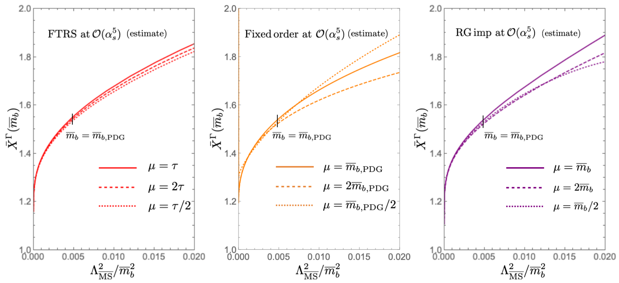
We compare ${\bar{X}}^{\Gamma}$ by the FTRS calculation with the fixed-order (FO) and RG-improved calculations. Explicitly, we define

	$\displaystyle{\bar{X}}^{\Gamma}_{\rm FO}(\overline{m}_{b})=\overline{m}_{b}\left[1+\sum_{n=0}^{2}\bar{g}_{n}(\mu_{0}/\overline{m}_{b})\alpha_{s}(\mu_{0})^{n+1}\right],$		(93)
	$\displaystyle{\bar{X}}^{\Gamma}_{\rm RG}(\overline{m}_{b})=\overline{m}_{b}\left[1+\sum_{n=0}^{2}\bar{g}_{n}(1)\alpha_{s}(\overline{m}_{b})^{n+1}\right].$		(94)

Fig. 8 shows a comparison of ${\bar{X}}^{\Gamma}_{\rm FTRS}$ , ${\bar{X}}^{\Gamma}_{\rm FO}$ and ${\bar{X}}^{\Gamma}_{\rm RG}$ . There are no significant differences in the scale dependence between them. The scale dependence of ${\bar{X}}^{\Gamma}_{\rm FTRS}$ at the current accuracy is still rather large, where the corrections up to ${\cal O}(\alpha_{s}^{3})$ are known. If the size of the $u=1$ renormalon is large in the original perturbative series, we expect that the convergence behavior of ${\bar{X}}^{\Gamma}_{\rm FTRS}$ is better than ${\bar{X}}^{\Gamma}_{\rm FO}$ or ${\bar{X}}^{\Gamma}_{\rm RG}$ , since we have eliminated it from the former.

We make an estimate of higher order results by including log dependent terms, dictated by the RGE, at the 5-loop level. We perform RG improvement of the perturbative series in $\tau$ space rather than $1/\overline{m}_{b}$ space, in accordance with the construction that there are no IR renormalons in the $\tau$ -space quantity. (Note that RG improvements in two spaces are not equivalent when we do not know the exact perturbative coefficient of the non-logarithmic term. In this treatment, the $u=1$ renormalon is induced in the perturbative series in $1/\overline{m}_{b}$ space. Then, ambiguities arise in ${\bar{X}}^{\Gamma}_{\rm FO}$ and ${\bar{X}}^{\Gamma}_{\rm RG}$ .) Fig. 8 shows a comparison of these 5-loop estimates. If $\overline{m}_{b}$ is around the physical mass of the $b$ quark, the scale dependence of the FTRS calculation is slightly better than the fixed-order and RG-improved calculations. Nevertheless, we cannot see significant differences between these three cases. In particular, the scale dependence of ${\bar{X}}^{\Gamma}_{\rm FO}$ and ${\bar{X}}^{\Gamma}_{\rm RG}$ is smaller than that of the FTRS result at the NLL level (see ref. [25]).

The above observations are consistent with the possibility that the size of the $u=1$ renormalon is small for this partial decay width. However, in order to estimate the size of the $u=1$ renormalon reliably, we need more terms of the perturbative series. On the other hand, in the lower mass range $\Lambda_{\rm\overline{MS}}^{2}/\overline{m}_{b}^{2}\gtrsim 0.01$ ( $\overline{m}_{b}\lesssim$ 3 GeV), we find a better convergence by the FTRS method than the usual fixed-order or RG-improved calculations. This can be due to circumventing the unphysical singularity of the running coupling constant in the FTRS method. It may indicate that we can make use of our method to lighter flavor observables (e.g. $D$ meson decay width).

In this analysis, although we use the $\overline{\rm MS}$ mass, it has been known that the use of other short distance masses can lead to better convergence of the perturbative series. This is because the $\overline{\rm MS}$ mass is far from the “physical” mass and needs a large perturbative correction to approximate it. In this study, we choose the $\overline{\rm MS}$ mass in order to use the FTRS method straightforwardly; if we instead use other short distance masses, additional issues arise, e.g., how to treat a factorization scale, which is introduced in many short distance masses but is not considered in the FTRS method. In addition, the disadvantage of the poor convergence can be compensated once the perturbative series of the decay and the mass relation are known to sufficiently high orders. In this regard, we showed results using estimated higher order perturbative series in Fig. 6. Thus we use the $\overline{\rm MS}$ mass for the first test of our formulation. Nevertheless, the use of other short distance masses may improve our result. We leave it as our future investigation.

5 Observable III : $B$ , $D$ meson masses

In this section we analyze the masses of the $B$ and $D$ mesons by the OPE in HQET ( $H=B^{(*)},D^{(*)}$ ). The renormalons at $u=1/2$ and $u=1$ , corresponding to the ${\cal O}(\Lambda_{\rm QCD})$ and ${\cal O}(\Lambda_{\rm QCD}^{2})$ renormalons, are subtracted simultaneously. We check consistency with theoretical expectations and extract the non-perturbative parameters $\bar{\Lambda}$ , $\mu^{2}_{\pi}$ using the $B^{(*)},D^{(*)}$ masses and our current knowledge of $\overline{m}_{b}$ , $\overline{m}_{c}$ , $\alpha_{s}(M_{Z})$ .

5.1 OPE of $H$ meson mass in HQET

The OPE of the $H$ mass is given by [45]

M_{H,\,\rm OPE}^{(s)}=m_{h}+\bar{\Lambda}+\frac{\mu^{2}_{\pi}}{2m_{h}}+w(s)X_{\rm cm}^{H}(m_{h})\frac{\mu^{2}_{G}}{2m_{h}}+{\cal O}\Big(\frac{\Lambda_{\rm QCD}^{3}}{m_{h}^{2}}\Big)\,,

(95)

where $s=0,1$ denotes the spin of $H$ ; $m_{h}$ represents the pole mass of the heavy quark ( $h=b,c$ ). $\bar{\Lambda}$ is an ${\cal O}(\Lambda_{\rm QCD})$ non-perturbative parameter defined by

\bar{\Lambda}=\lim_{m_{h}\to\infty}\big[m_{H}-m_{h}\big]\,,

(96)

which represents the contribution from light degrees of freedom. To give an unambiguous definition of $\bar{\Lambda}$ we need to specify which regularization is applied to the pole mass $m_{h}$ , and we adopt the PV prescription here. $\mu^{2}_{\pi}$ and $\mu^{2}_{G}$ are defined by eq. (81). The Wilson coefficient of $\mu^{2}_{\pi}$ is exactly one according to the reparametrization invariance, while that of $\mu^{2}_{G}$ is known up to order ${\cal O}(\alpha_{s}^{3})$ [48]. The spin dependent weight is given by $w(0)=1,\,w(1)=-1/3$ . Due to the heavy quark symmetry of HQET, the non-perturbative parameters $\bar{\Lambda}$ , $\mu^{2}_{\pi}$ , $\mu^{2}_{G}$ have common values for $H=B$ and $D$ [40].

We project out $\mu^{2}_{G}$ by taking the linear combination,

	$\displaystyle\overline{M}_{H,\,\rm OPE}$	$\displaystyle\equiv$	$\displaystyle\frac{M_{H,\,\rm OPE}^{(0)}+3M_{H,\,\rm OPE}^{(1)}}{4}$		(97)
		$\displaystyle=$	$\displaystyle m_{h}+\bar{\Lambda}+\frac{\mu^{2}_{\pi}}{2m_{h}}+{\cal O}\Big(\frac{\Lambda_{\rm QCD}^{3}}{m_{h}^{2}}\Big).$		(97)

The IR renormalons in the pole mass $m_{h}$ are canceled by $\bar{\Lambda}$ , $\mu_{\pi}^{2}$ , $\cdots$ in the OPE framework. We separate the ${\cal O}(\Lambda_{\rm QCD})$ and ${\cal O}(\Lambda_{\rm QCD}^{2})$ renormalons from $m_{h}$ by the FTRS method. Since the Wilson coefficients of $\bar{\Lambda}$ and $\mu_{\pi}^{2}$ are exactly one and the ${\cal O}(\Lambda_{\rm QCD})$ and ${\cal O}(\Lambda_{\rm QCD}^{2})$ renormalons have no logarithmic corrections, these renormalons are completely removed within our formalism (without using the extended formalism explained in App. B).

5.2 ${dm_{b}}/d{\overline{m}_{b}}$ : FTRS, fixed-order and RG-improved calculations

First, we compare the FTRS method with the fixed-order and RG-improved calculations. We are interested in the effects of the $u=1$ [ ${\cal O}(\Lambda_{\rm QCD}^{2})$ ] renormalon in particular. Hence, we calculate $dm_{b}/d\overline{m}_{b}$ , which is free from the $u=1/2$ [ ${\cal O}(\Lambda_{\rm QCD})$ ] renormalon ambiguity even in the fixed-order and RG-improved calculations. In this subsection, we use the perturbative series for the $b$ quark pole mass in the theory with four massless quarks ( $u,d,s,c$ ). In the OPE analysis in the following subsections, however, we need to pay attention to the treatment of finite (non-zero) mass effects of the $c$ quark, in order to be compatible with the flavor universality of the non-perturbative matrix elements (heavy quark symmetry). Since we do not need to care about the flavor universality in this subsection, we use the simple perturbative series for clarity.

We construct ${m_{b}^{\rm FTRS}}(\overline{m}_{b})$ as follows. To subtract the ${\cal O}(\Lambda_{\rm QCD})$ and ${\cal O}(\Lambda_{\rm QCD}^{2})$ renormalons from $m_{b}$ , we set the parameters $(a,u^{\prime})=(2,-1/2)$ . The renormalons at $u=1/2,1,3/2,\cdots$ are suppressed in momentum space. Explicitly, we have

{m_{b}^{\rm FTRS}}(\overline{m}_{b})=\overline{m}_{b}+m_{b,0}(\overline{m}_{b})+m_{b,\rm pow}(\overline{m}_{b}),

(98)

m_{b,0}(\overline{m}_{b})=-\frac{\sqrt{\overline{m}_{b}}}{2\pi^{2}}\int_{0}^{\infty}dt\,t\,e^{-t/\sqrt{\overline{m}_{b}}}{\rm Im}\,[\tilde{c}_{m}(\tau=it)]

(99)

m_{b,\rm pow}(\overline{m}_{b})=\frac{\sqrt{\overline{m}_{b}}}{4\pi^{2}i}\int_{C_{*}}d\tau\,\tau\biggl(1-\frac{\tau^{2}}{2\overline{m}_{b}}\biggr)\tilde{c}_{m}(\tau)\,,

(100)

where $c_{m}(\overline{m})$ is defined in eq. (83). After resummation of the artificial UV renormalons at $u=-1/4$ and $-3/4$ , $\tilde{c}_{m}(\tau)$ in the $\rm N^{3}LL$ approximation is calculated from ${m_{b}}/{\overline{m}_{b}}-1=\sum_{n=0}^{3}d_{n}(\mu/\overline{m}_{b})\alpha_{s}^{n+1}$ as

	$\displaystyle\tilde{c}_{m}(\tau)\biggr\|_{\rm N^{3}LL}=\frac{4\pi}{\tau}\Biggl[\biggl[\sin(2{\pi}u_{})\Gamma(4u_{})-\Big(\frac{1}{4}\frac{1}{u_{}+1/4}-\frac{1}{24}\frac{1}{u_{}+3/4}\Big)\biggr]_{u_{*}\to\hat{H}}$
	$\displaystyle~~~~~~~~~~~~~~~~~~~~~~~~~\times\sum_{n=0}^{\infty}d_{n}\alpha_{s}(\tau^{2})^{n+1}\Biggr]_{\text{up to ${\cal O}(\alpha_{s}(\tau^{2})^{4})$}}$
	$\displaystyle~~~~~~~~~~~~~~~~~~~~~~+\frac{4\pi}{\tau}\int_{0}^{1}\frac{dv}{2v}\,\Big(v^{1/2}-\frac{1}{6}v^{3/2}\Big)\sum_{n=0}^{3}d_{n}\alpha_{s}(\tau^{2}/v)^{n+1}$
	$\displaystyle~~~~~\approx\frac{4\pi}{\tau}\Bigg[0.2658a_{\tau}+0.6730a_{\tau}^{2}+1.803a_{\tau}^{3}+3.290a_{\tau}^{4}$
	$\displaystyle~~~~~~~~+\int_{0}^{1}\frac{dv}{2v}\,\Big(v^{1/2}-\frac{1}{6}v^{3/2}\Big)\Big(0.4244a_{\tau,v}+0.9401a_{\tau,v}^{2}+3.039a_{\tau,v}^{3}+12.65a_{\tau,v}^{4}\Big)\Bigg],$
			(101)

where $a_{\tau}=\alpha_{s}({\tau}^{2}),a_{\tau,v}=\alpha_{s}(\tau^{2}/v)$ . In this analysis (in Sec. 5.2), we use $d_{n}=\tilde{d}_{n}{(n_{l}=4)}$ of eqs. (147)–(149) without finite mass corrections inside loops $(m_{c}\to 0)$ , i.e., eq. (150). Scale variation in the numerical analysis is studied according to the same procedure in Sec 3.2.

We compare $dm_{b}/d\overline{m}_{b}$ by the FTRS calculation with the fixed-order (FO) and RG-improved calculations. Explicitly, we define

	$\displaystyle m_{b}^{\rm FO}(\overline{m}_{b})=\overline{m}_{b}\left[1+\sum_{n=0}^{3}d_{n}(\mu_{0}/\overline{m}_{b})\alpha_{s}(\mu_{0})^{n+1}\right],$		(102)
	$\displaystyle m_{b}^{\rm RG}(\overline{m}_{b})=\overline{m}_{b}\left[1+\sum_{n=0}^{3}d_{n}(1)\alpha_{s}(\overline{m}_{b})^{n+1}\right].$		(103)

We take the derivative of $m_{b}$ with respect to $\overline{m}_{b}$ . Then the ${\cal O}(\Lambda_{\rm QCD})$ renormalon ambiguity is absent in all three quantities, while only the FTRS calculation is free from the $u=1$ renormalon. Fig. 9 compares the scale dependence. For each hypothetical value of $\overline{m}_{b}$ , the scale $\mu$ is varied between $[\tau^{2}/2,2\tau^{2}]$ , $[\mu_{0}/2,2\mu_{0}]$ and $[\overline{m}_{b}/2,2\overline{m}_{b}]$ in the FTRS, fixed-order and RG-improved calculations, respectively. Here, we choose $\mu_{0}=17.71\Lambda_{\rm\overline{MS}}$ , which coincides with the minimal sensitivity scale of $dm_{b}^{\rm FO}/d\overline{m}_{b}$ for $\overline{m}_{b}=\overline{m}_{b,\rm PDG}=4.18$ GeV [52]. The bottom-right figure shows the scale dependence of each calculation near $\overline{m}_{b}=\overline{m}_{b,\rm PDG}$ . There is no significant difference between them. It is consistent with the result of the previous study that the $u=1$ renormalon is small and hardly visible from the currently known perturbative coefficients [28].

5.3 Internal quark mass effects in pole– $\overline{\rm MS}$ mass relation

First, we review a non-trivial aspect in eliminating the $u=1/2$ and $u=1$ renormalons in the pole masses, $m_{b}$ and $m_{c}$ , by the universal parameters $\bar{\Lambda}$ and $\mu^{2}_{\pi}$ . After that we consider an application to the FTRS method.

Naively one may expect that the IR structure of the bottom (charm) quark is described well in the theory with $n_{l}=4$ ( $n_{l}=3$ ) massless quarks. ( $n_{l}$ denotes the number of massless quarks.) Hence, the renormalons of the different quark pole masses could originate from the different IR structures. It is known, however, that internal massive quarks in loops do not contaminate the IR structure, that is, the internal charm quark with a non-zero (finite) mass does not contribute to the renormalon divergences of the bottom quark pole mass. Therefore, to be consistent with the universality of the non-perturbative parameters, we need to consider the theory with three massless quarks plus massive charm and bottom quarks in the OPE analysis. In this theory the $B$ and $D$ mesons share the same light sector and hence the same renormalon structure, and we can subtract the renormalons consistently with the universality of the non-perturbative matrix elements in HQET.

This feature is demonstrated in the large- $\beta_{0}$ approximation with a finite charm quark mass included in loops, as follows. The bottom quark pole mass in this approximation is given by the loop momentum integration,

\frac{m_{b,\rm pole}-\overline{m}_{b}}{\overline{m}_{b}}=\int d^{4}k\,F(k,\overline{m}_{b})\,\frac{1}{k^{2}}\,\frac{\alpha_{s}^{(4)}(\mu)}{1-\alpha_{s}^{(4)}(\mu)\Pi(k^{2},\overline{m}_{c})},

(104)

where $F(k,\overline{m}_{b})$ is a kinematic function and $\alpha_{s}^{(n_{f})}$ represents the strong coupling constant of the $n_{f}$ -flavor theory. We have rewritten $\alpha_{s}^{(5)}$ by $\alpha_{s}^{(4)}$ , which absorbs the effect of the bottom quark loops. $\Pi(k^{2},\overline{m}_{c})$ is the one-loop vacuum polarization which includes a massive charm quark loop,

\Pi(k^{2},\overline{m}_{c})=\Pi_{\rm light}(k^{2})+\Pi_{c}(k^{2},\overline{m}_{c}),

(105)

where $\Pi_{\rm light}$ represents the contribution from the light degrees of freedom (gluons and massless quarks) while $\Pi_{c}$ represents the charm quark contribution. In the IR region $k^{2}\simeq 0$ , they are given by

\Pi_{\rm light}(k^{2})=b_{0}^{(3)}\left[\log\left(-\frac{\mu^{2}}{k^{2}}\right)+\frac{5}{3}\right],

(106)

\Pi_{c}(k^{2},\overline{m}_{c})=-\frac{1}{6\pi}\log\left(\frac{\mu^{2}}{\overline{m}_{c}^{2}}\right)+{\cal O}\left(\frac{k^{2}}{\overline{m}_{c}^{2}}\right)\,,

(107)

with $b_{0}^{(n_{l})}=(11-2n_{l}/3)/(4\pi)$ . $\Pi_{c}$ does not have $\log(k^{2})$ behavior in the IR region [49], since the charm quark mass works as an IR regulator in the fermion loop integration. As a result the charm quark contributions do not give renormalons.

We can absorb the $\log(\mu^{2}/\overline{m}_{c}^{2})$ term in eq. (107) if we use the coupling constant of the 3-flavor theory,

\displaystyle\frac{\alpha_{s}^{(4)}(\mu)}{1-\alpha_{s}^{(4)}(\mu)\Pi(k^{2},\overline{m}_{c})}=\frac{\alpha_{s}^{(3)}(\mu)}{1-\alpha_{s}^{(3)}(\mu)\Pi_{\rm light}(k^{2})+\mathcal{O}(k^{2}/\overline{m}_{c}^{2})},

(108)

due to the one loop threshold correction in the $\overline{\rm MS}$ scheme

\frac{1}{\alpha_{s}^{(4)}(\mu)}=\frac{1}{\alpha_{s}^{(3)}(\mu)}-\frac{1}{6\pi}\log(\mu^{2}/\overline{m}_{c}^{2}).

(109)

After this rewriting, one can clearly see that the renormalon we encounter coincides with the one in the $n_{f}=3$ theory:

\frac{m_{b,\rm pole}-\overline{m}_{b}}{\overline{m}_{b}}\approx K\sum_{n=0}^{\infty}(2b_{0})^{n}n![\alpha_{s}^{(3)}(\overline{m}_{b})]^{n+1}\,.

(110)

In fact, it was pointed out that one should use $\alpha_{s}^{(3)}$ rather than $\alpha_{s}^{(4)}$ as the expansion parameter [50].

We now show that, in order for the FTRS method to work with our parameter choice $(a,u^{\prime})=(2,-1/2)$ , it is necessary to express the perturbative series in the 3-flavor coupling constant. In fact, renormalons remain in $\tau$ space if we use the 4-flavor coupling constant. With the 4-flavor coupling constant, from eqs. (106) and (107), the Borel transform close to the first IR renormalon is given by

B^{\text{4-flavor}}(u)\approx\left(\frac{\mu^{2}e^{5/3}}{\overline{m}_{b}^{2}}\right)^{\frac{b_{0}^{(3)}}{b_{0}^{(4)}}u}\left(\frac{\mu^{2}}{\overline{m}_{c}^{2}}\right)^{\frac{u}{6\pi b_{0}^{(4)}}}\frac{1}{1-2\frac{b_{0}^{(3)}}{b_{0}^{(4)}}u},

(111)

where $u=b_{0}^{(4)}t$ . The singularity is located at $u=b_{0}^{(4)}/(2b_{0}^{(3)})$ . Then the Borel transform of the $\tau$ -space perturbative series is given by

	$\displaystyle\tilde{B}^{\text{4-flavor}}(u)\approx\left(\frac{\mu^{2}e^{5/3}}{\tau^{2a}}\right)^{\frac{b_{0}^{(3)}}{b_{0}^{(4)}}u}\left(\frac{\mu^{2}}{\overline{m}_{c}^{2}}\right)^{\frac{u}{6\pi b_{0}^{(4)}}}\frac{1}{1-2\frac{b_{0}^{(3)}}{b_{0}^{(4)}}u}\sin\left(\pi a\left(\frac{b_{0}^{(3)}}{b_{0}^{(4)}}u+u^{\prime}\right)\right)$
	$\displaystyle~~~~~~~~~~~~~~~~~~~\times\Gamma\left(2a\left(\frac{b_{0}^{(3)}}{b_{0}^{(4)}}u+u^{\prime}\right)+2\right).$		(112)

The singularity at $u=b_{0}^{(4)}/[2b_{0}^{(3)}]$ cannot be eliminated in $\tau$ space with the parameter set $(a,u^{\prime})=(2,-1/2)$ , which is chosen to eliminate the $u=1/2$ renormalon.¹⁶¹⁶ 16 One can eliminate the renormalons by setting the parameters to $(a,u^{\prime})=(2,-b_{0}^{(3)}/(2b_{0}^{(4)}))$ . Using the 3-flavor coupling constant instead, the Borel transform has the $u=1/2$ renormalon,

B^{\text{3-flavor}}(u)\approx\left(\frac{\mu^{2}e^{5/3}}{\overline{m}_{b}^{2}}\right)^{u}\frac{1}{1-2u},

(113)

hence, we can properly eliminate the $u=1/2$ renormalon in $\tau$ space with $(a,u^{\prime})=(2,-1/2)$ :

	$\displaystyle\tilde{B}^{\text{3-flavor}}(u)\approx\left(\frac{\mu^{2}e^{5/3}}{\overline{m}_{b}^{2}}\right)^{u}\frac{1}{1-2u}\sin\left(\pi a\left(u+u^{\prime}\right)\right)\Gamma\left(2a\left(u+u^{\prime}\right)+2\right)$
	$\displaystyle~~~~~~~~~~~~~\approx\mathcal{O}\left(\left(u-\frac{1}{2}\right)^{0}\right).$		(114)

Based on the above consideration, we will use $\alpha_{s}^{(3)}$ in the following calculations. In App. A, we give the explicit perturbative series of the pole- $\overline{\rm MS}$ mass relation for the bottom and charm quarks [eqs. (151) and (152)] in terms of $\alpha_{s}^{(3)}$ . Here we use the most precise perturbative coefficients available today: in the 5-flavor theory, the finite charm mass effects are included in the bottom pole mass, while the non-decoupling effects of the bottom mass are included in the charm pole mass, respectively, up to the $\mathcal{O}(\alpha_{s}^{3})$ order [51]. Then we use the matching relations to rewrite the coupling constant $\alpha_{s}^{(5)}\to\alpha_{s}^{(3)}$ and the $\overline{\rm MS}$ mass $\overline{m}_{c}^{(5)}\to\overline{m}_{c}^{(4)}$ (which is needed to use the input mass parameter by the Particle Data Group [52].) The perturbative series are numerically close to each other and also they are close to the pole- $\overline{\rm MS}$ mass relation for a heavy quark with three-massless quarks only [eq. (153)]. These features indicate that these two perturbative series indeed exhibit the renormalon divergence of the $n_{l}=3$ flavor theory, as expected from the above argument in the large- $\beta_{0}$ approximation. It is especially noteworthy that the renormalon behavior of the bottom quark pole mass is dominated only by the three light flavors, whose typical scales are less than $\Lambda_{\rm QCD}$ , and not affected by the charm quark, also beyond the large- $\beta_{0}$ approximation. For this reason, we approximate the $\mathcal{O}(\alpha_{s}^{4})$ coefficients of the finite mass corrections, which are not known today, by that of the heavy quark pole mass with three massless quarks only, for both bottom and charm quarks, i.e., $\delta d_{3}=0$ (when expressed by $\alpha_{s}^{(3)}$ ).

5.4 Extracting $\bar{\Lambda}_{\rm FTRS},\,(\mu^{2}_{\pi})_{\rm FTRS}$

Using $m_{h}^{\rm FTRS}$ , we define

\overline{M}_{H,\,\rm OPE}=m_{h}^{\rm FTRS}+\bar{\Lambda}_{\rm FTRS}+\frac{(\mu^{2}_{\pi})_{\rm FTRS}}{2m_{h}^{\rm FTRS}}+{\cal O}\Big(\frac{\Lambda_{\rm QCD}^{3}}{m_{h}^{2}}\Big).

(115)

$m_{b}^{\rm FTRS}$ ( $m_{c}^{\rm FTRS}$ ) is given by eqs. (98)–(101) with $d_{n}=\tilde{d}_{n}({n_{l}=3})+\delta d_{n}$ in eq. (151) (eq. (152)) up to ${\cal O}(\alpha_{s}^{4})$ , which includes non-zero mass corrections from the charm quark (bottom quark). Explicitly $\tilde{c}_{m}$ are given by

	$\displaystyle\tilde{c}_{m}(\tau)\biggr\|_{m_{b},\,{\rm N^{3}LL}}\!\!\!\!\!\!\!$		$\displaystyle\approx\frac{4\pi}{\tau}\Bigg[0.2658a_{\tau}+0.7407a_{\tau}^{2}+2.240a_{\tau}^{3}+5.096a_{\tau}^{4}$
			$\displaystyle+\int_{0}^{1}\frac{dv}{2v}\,\Big(v^{1/2}-\frac{1}{6}v^{3/2}\Big)\Big(0.4244a_{\tau,v}+1.037a_{\tau,v}^{2}+3.744a_{\tau,v}^{3}+17.44a_{\tau,v}^{4}\Big)\Bigg],$

	$\displaystyle\tilde{c}_{m}(\tau)\biggr\|_{m_{c},\,{\rm N^{3}LL}}\!\!\!\!\!\!\!$		$\displaystyle\approx\frac{4\pi}{\tau}\Bigg[0.2658a_{\tau}+0.7447a_{\tau}^{2}+2.252a_{\tau}^{3}+5.080a_{\tau}^{4}$
			$\displaystyle+\int_{0}^{1}\frac{dv}{2v}\,\Big(v^{1/2}-\frac{1}{6}v^{3/2}\Big)\Big(0.4244a_{\tau,v}+1.044a_{\tau,v}^{2}+3.757a_{\tau,v}^{3}+17.44a_{\tau,v}^{4}\Big)\Bigg],$

where $a_{\tau}=\alpha_{s}({\tau}^{2})$ , $a_{\tau,v}=\alpha_{s}(\tau^{2}/v)$ . Scale variation in the numerical analysis is studied according to the same procedure in Sec 3.2.

We compare $\overline{M}_{B,\rm OPE}$ and $\overline{M}_{D,\rm OPE}$ with the experimental values

\overline{M}_{B,{\rm exp}}=5.313\,{\rm GeV},\quad\overline{M}_{D,{\rm exp}}=1.971\,{\rm GeV},

(118)

to determine the values of $\bar{\Lambda}_{\rm FTRS}$ and $(\mu^{2}_{\pi})_{\rm FTRS}$ . The input parameters of $\overline{M}_{H,\,\rm OPE}$ are taken as [52],

\overline{m}_{b}^{(5)}=4.18^{+0.03}_{-0.02}\,{\rm GeV},\quad\overline{m}_{c}^{(4)}=1.27\pm 0.02\,{\rm GeV},

(119)

and

\Lambda_{\rm\overline{MS}}^{n_{f}=3}=0.332\pm{0.015}\,\rm GeV\,,

(120)

corresponding to $\alpha_{s}^{n_{f}=5}(M_{Z})=0.1179\pm 0.0010$ . The above $\Lambda_{\rm\overline{MS}}$ is obtained with the four-loop beta function and three-loop matching relation. We use the above value ${\Lambda_{\rm\overline{MS}}^{n_{f}=3}}|_{\text{4-loop}}$ as the input of $\Lambda_{\rm\overline{MS}}^{n_{f}=3}|_{\text{5-loop}}$ ; we discard the difference between ${\Lambda_{\rm\overline{MS}}^{n_{f}=3}}|_{\text{4-loop}}$ and ${\Lambda_{\rm\overline{MS}}^{n_{f}=3}}|_{\text{5-loop}}$ . The result reads

	$\displaystyle\bar{\Lambda}_{\rm FTRS}=0.495(15)_{\mu}(49)_{\overline{m}_{b}}(12)_{\overline{m}_{c}}(13)_{\alpha_{s}}(0)_{\rm f.m.}\text{GeV}\,,$		(121)
	$\displaystyle(\mu_{\pi}^{2})_{\rm FTRS}=-0.12(13)_{\mu}(15)_{\overline{m}_{b}}(11)_{\overline{m}_{c}}(4)_{\alpha_{s}}(0)_{\rm f.m.}\text{GeV}^{2},$		(122)

where the errors denote, respectively, that from the scale dependence for $\tau^{2}/2\leq\mu\leq 2\tau^{2}$ , from the errors of the input $\overline{m}_{b}$ , $\overline{m}_{c}$ , $\alpha_{s}$ , and from turning off the $\overline{m}_{c}/\overline{m}_{b}$ corrections of $d_{2}$ and use $d_{2}(n_{l}=3)$ . We note that the removal of the finite mass effects on the $\mathcal{O}(\alpha_{s}^{3})$ coefficient does not change the result at the precision level we work. Combining the errors in quadrature, we obtain

\displaystyle\bar{\Lambda}_{\rm FTRS}=0.495\pm 0.053~\text{GeV}\,,~~~~~(\mu_{\pi}^{2})_{\rm FTRS}=-0.12\pm 0.23~\text{GeV}^{2}\,.

(123)

The error from the scale dependence is a measure of perturbative ambiguity. With our parameter choice, the renormalons at $u=1/2$ and $1$ should be absent from our result. For $\bar{\Lambda}_{\rm FTRS}$ , about 3 per cent error shows successful subtraction of the $u=1/2$ renormalon. On the other hand, the scale dependence of $(\mu_{\pi}^{2})_{\rm FTRS}$ is not smaller than ${\cal O}(\Lambda_{\rm QCD}^{2})$ . We estimate that this is not because of the contribution from the $u=1$ renormalon but due to the insufficient number of known terms of the perturbative series. A 5-loop examination by using the 5-loop beta function combined with the estimated 5-loop coefficient in the large- $\beta_{0}$ approximation [ $d_{n}$ ’s are given by eq. (151) and eq. (152) up to ${\cal O}(\alpha_{s}^{5})$ ] gives the following result:

\bar{\Lambda}^{\rm(est)}_{\rm FTRS}\Big|_{\rm 5-loop}=0.488(4)_{\mu}\text{GeV}\,,\,~~(\mu_{\pi}^{2})^{\rm(est)}_{\rm FTRS}\Big|_{\rm 5-loop}=-0.09(7)_{\mu}\text{GeV}^{2}.

(124)

This indicates that the scale dependence of $\bar{\Lambda}_{\rm FTRS}$ and $(\mu_{\pi}^{2})_{\rm FTRS}$ can be straightforwardly reduced at higher orders.

As mentioned above, the inclusion of the finite mass effects at $\mathcal{O}(\alpha_{s}^{3})$ gives only tiny effects. It would be interesting to examine what happens if we completely neglect the finite mass effects. With the perturbative series of a heavy quark with three massless flavors only, for both bottom and charm quarks [eq. (153)], we obtain $\bar{\Lambda}_{\rm FTRS}\big|_{n_{l}=3}=0.493\,\text{GeV}\,,\,(\mu_{\pi}^{2})_{\rm FTRS}\big|_{n_{l}=3}=-0.11\,\text{GeV}^{2},$ where $\mu=\tau^{2}$ . The values hardly change from the above results [eqs. (121) and (122)], where we take into account the finite bottom and charm mass effects.

Let us compare our results for $\bar{\Lambda}$ and $\mu_{\pi}^{2}$ with other determinations. Ref. [12] obtained

\displaystyle\bar{\Lambda}_{\rm PV}=0.435(31)~{\rm GeV}\,,~~~(\mu_{\pi}^{2})_{\rm PV}=0.05(22)~{\rm GeV}^{2}\,.

(125)

In this fit, only the ${\cal O}(\Lambda_{\rm QCD})$ renormalon is subtracted, while the ${\cal O}(1/m_{h})$ corrections are included. They estimate that the error of $\mu_{\pi}^{2}$ originates from the ${\cal O}(\Lambda_{\rm QCD}^{2})$ renormalon. However, our analysis indicates that it is rather due to the lack of known perturbative coefficients, since the size of the ${\cal O}(\Lambda_{\rm QCD}^{2})$ renormalon is small. (This is estimated by the comparison between the predictions with and without the ${\cal O}(\Lambda_{\rm QCD}^{2})$ renormalon subtraction.) Ref. [28] obtained

\displaystyle\bar{\Lambda}_{\rm PV}=477(\mu)^{-8}_{+17}(Z_{m})^{+11}_{-12}(\alpha_{s})^{-8}_{+9}({\cal O}(1/m_{h}))^{+46}_{-46}~{\rm MeV}\,,

(126)

in which only the ${\cal O}(\Lambda_{\rm QCD})$ renormalon is subtracted and the ${\cal O}(1/m_{h})$ corrections are ignored (including the $\mu_{\pi}^{2}$ term). Both of these determinations use the PV scheme and are consistent with our determination within the assigned errors.

To further examine the convergence property of the FTRS method, we perform an FTRS calculation of the bottom and charm quark pole masses (relevant to the above study) by changing the order of the approximation. The result is as follows.

$\displaystyle{\rm N^{2}LL}$	$\displaystyle:~~~~~~$	$\displaystyle m_{b}^{\rm FTRS}=4.811(27)~\text{GeV},~~~m_{c}^{\rm FTRS}=1.527(34)~\text{GeV},$	(127)
$\displaystyle{\rm N^{3}LL}$	$\displaystyle:~~~~~~$	$\displaystyle m_{b}^{\rm FTRS}=4.831~\,(8)~\text{GeV},~~~m_{c}^{\rm FTRS}=1.516(31)~\text{GeV},$	(128)
$\displaystyle{\rm N^{4}LL}$	$\displaystyle{\rm(estimate)}:~$	$\displaystyle m_{b}^{\rm FTRS}=4.835~\,(6)~\text{GeV},~~~m_{c}^{\rm FTRS}=1.513(20)~\text{GeV}.$	(129)

The numbers inside parentheses denote the errors from scale variation within $\mu\in[\tau/2,2\tau]$ . In the N⁴LL estimate, we use the coefficient of the ${\cal O}(\alpha_{s}^{5})$ term in the large- $\beta_{0}$ approximation. This result indicates convergence of the perturbative series.

6 Summary and conclusions

Towards high precision calculations of QCD effects, it is important to establish a formulation incorporating IR renormalon cancellation, beyond the ${\cal O}(\Lambda_{\rm QCD})$ renormalon of the quark pole mass. In this paper, we advocate a new method (FTRS method) within the OPE framework, which realizes separation and cancellation of IR renormalons of a general observable. The method can cancel multiple renormalons simultaneously. We presented first test analyses of this method applied to three observables (Adler function, $B$ -meson semileptonic decay width, and $B$ , $D$ meson masses). We confirmed good consistency with theoretical expectations. In particular we determined $\bar{\Lambda}$ and $\mu^{2}_{\pi}$ by subtracting ${\cal O}(\Lambda_{\rm QCD})$ and ${\cal O}(\Lambda_{\rm QCD}^{2})$ renormalons simultaneously for the first time.

The FTRS method is based on the following idea and construction. We express the leading Wilson coefficient of an observable by a one-parameter integral, in which the IR renormalons of the integrand are suppressed. The integral is constructed by the Fourier transform. Due to a property of the Fourier transform, one can adjust parameters in the transform to suppress the desired renormalons of the integrand. Then one can combine the RG and contour deformation to separate and subtract the renormalons of the observable. The result coincides with the renormalon-subtracted Wilson coefficient in the PV prescription at large orders. This is a generalization of the method used for the static QCD potential, for which ample tests have already been carried out.

One might have guessed that, in order to separate and eliminate renormalons of a Wilson coefficient by organizing it in $1/Q^{2}$ expansion, analyses of the IR structures of the individual observables are mandatory by investigating the details of loop integrals (e.g., using the expansion-by-regions technique). As it turned out, it is possible to construct the necessary expansion of the Wilson coefficient without knowing the deep structures. The only knowledge of the usual perturbative coefficients is sufficient. The obtained formula has a concise form. For instance, we do not need to perform fits to extract the normalization of individual renormalons.

It is also interesting that one can derive the same formula in another way, which is more closely connected to the Wilsonian picture, by introducing a factorization scale in the artificial “momentum space.” It may be useful to develop a physical insight into the FTRS formulation.

In the latter part of the paper, we performed test analyses of the FTRS method. In the first example, we subtracted the ${\cal O}(\Lambda_{\rm QCD}^{4})$ renormalon from the Adler function so that the gluon condensate is also well defined. The scale dependence of the FTRS calculation is smaller than the fixed-order and RG-improved calculations, showing improvement of convergence by the renormalon subtraction. From comparison with a phenomenological model, consistency with the OPE is observed. Then we estimated the values of the gluon condensate and $\Lambda_{\rm\overline{MS}}^{n_{f}=2}$ from this comparison, the latter of which agrees with its lattice determinations from various observables. The matching was performed in the range where the non-perturbative $1/Q^{4}$ contribution plays a significant role, and the consistency with the OPE seems non-trivial. Our estimate of the 5-loop correction indicates that we may need to take care of the $u=-1$ UV renormalon in the Adler function to improve accuracy by going to higher orders.

In the second example, we subtracted the ${\cal O}(\Lambda_{\rm QCD}^{2})$ renormalon from the $B\to X_{u}l\overline{\nu}$ decay width, after canceling the ${\cal O}(\Lambda_{\rm QCD})$ renormalons by using the $\overline{\rm MS}$ mass. Incorporating the recently calculated ${\cal O}(\alpha_{s}^{3})$ corrections, we scarcely observed differences in the scale dependence of the FTRS, fixed-order and RG-improved calculations. We estimated a higher-order correction using the 5-loop beta function. In this estimate the FTRS calculation showed smaller scale dependence than the fixed-order and RG-improved calculations. It indicates that we can improve accuracy at higher orders by the ${\cal O}(\Lambda_{\rm QCD}^{2})$ renormalon subtraction.

In the last example, we subtracted the ${\cal O}(\Lambda_{\rm QCD})$ and ${\cal O}(\Lambda_{\rm QCD}^{2})$ renormalons simultaneously from the $B$ and $D$ meson masses. We determined $\bar{\Lambda}$ and $\mu_{\pi}^{2}$ , which became well defined by the renormalon subtraction. With the perturbative corrections up to ${\cal O}(\alpha_{s}^{4})$ , we compared the derivative of the $b$ quark pole mass with respect to the $\overline{\rm MS}$ mass, $dm_{b}/d\overline{m}_{b}$ , between the FTRS calculation, fixed-order calculation, and RG-improved calculation. The scale dependence is similar (except when we choose a very small scale). This is consistent with the previous observation that the $u=1$ renormalon in the heavy quark pole mass is small. Comparing to the experimental values of the $B,\,D$ meson masses, we determined the universal non-perturbative parameters $\bar{\Lambda}_{\rm FTRS}$ and $(\mu_{\pi}^{2})_{\rm FTRS}$ taking the PDG values of $\overline{m}_{b},\,\overline{m}_{c},\,\alpha_{s}(M_{Z})$ as inputs. We obtained

\displaystyle\bar{\Lambda}_{\rm FTRS}=0.495\pm 0.053~\text{GeV}\,,~~~~~(\mu_{\pi}^{2})_{\rm FTRS}=-0.12\pm 0.23~\text{GeV}^{2}\,.

(130)

To ensure universality (heavy quark symmetry) of $\bar{\Lambda}_{\rm FTRS}$ and $(\mu_{\pi}^{2})_{\rm FTRS}$ we need to work in the theory with three massless plus massive $c$ , $b$ quarks consistently. Furthermore, expansion in the 3-flavor coupling constant $\alpha_{s}^{(3)}(\tau^{2})$ is necessary to fully eliminate the ${\cal O}(\Lambda_{\rm QCD})$ and ${\cal O}(\Lambda_{\rm QCD}^{2})$ renormalons in the FTRS method. The scale dependence of $\bar{\Lambda}_{\rm FTRS}$ is small (0.015 GeV), whereas $(\mu_{\pi}^{2})_{\rm FTRS}$ has relatively large scale dependence (0.13 GeV²) with respect to the ${\cal O}(\Lambda_{\rm QCD}^{2})$ renormalon subtraction. We estimate that the latter feature is due to the insufficient number of known perturbative coefficients. A 5-loop estimate indicates that the error would reduce if higher order perturbative calculation of the pole mass is achieved.

In all the above analyses we observed good consistency with theoretical expectations, such as better convergence and stability, by subtracting renormalons beyond the ${\cal O}(\Lambda_{\rm QCD})$ renormalon. Nevertheless, we need to know more terms of the relevant perturbative series in order to make conclusive statements about the effects of subtracting the renormalons. Our analyses also show that the 5-loop QCD beta function is a crucial ingredient in improving accuracies. Application of the FTRS method to the determination of fundamental physical parameters is under preparation. It is desirable that higher order perturbative calculations of Wilson coefficients will be advanced in conjunction. We thus anticipate that the FTRS method can be a useful theoretical tool for precision QCD calculations in the near future.

In these first analyses we used the FTRS method ignoring the $\log(Q)$ corrections and the anomalous dimensions $\gamma(\alpha_{s})$ of the subtracted renormalons. (Some of the renormalons have no corrections exactly.) In principle, these corrections can be incorporated using the method discussed in App. B. Its application to practical analyses is left to our future investigations.

Acknowledgements

Y.H. acknowledges support from GP-PU at Tohoku University. The work of Y.H. was also supported in part by Grant-in-Aid for JSPS Fellows (No. 21J10226) from MEXT, Japan. The works of Y.S. and H.T., respectively, were supported in part by Grant-in-Aid for scientific research (Nos. 20K03923 and 19K14711) from MEXT, Japan.

Appendix

Appendix A List of perturbative coefficients

In this appendix, we collect the perturbative coefficients necessary for the analyses in this paper.

The QCD $\beta$ function is known up to ${\cal O}(\alpha_{s}^{6})$ (5-loop accuracy) [37].

\beta(\alpha_{s})=-\sum_{i=0}^{4}b_{i}\alpha_{s}^{i+2},

(131)

b_{0}=\frac{1}{4\pi}\Big(11-\frac{2}{3}n_{f}\Big),\quad b_{1}=\frac{1}{(4\pi)^{2}}\Big(102-\frac{38}{3}n_{f}\Big),

(132)

b_{2}=\frac{1}{(4\pi)^{3}}\Big(\frac{2857}{2}-\frac{5033}{18}n_{f}+\frac{325}{54}n_{f}^{2}\Big),

(133)

	$\displaystyle b_{3}=\frac{1}{(4\pi)^{4}}\Big[\frac{149753}{6}$	$\displaystyle+$	$\displaystyle 3564\zeta_{3}-\Bigg(\frac{1078361}{162}+\frac{6508}{27}\zeta_{3}\Big)n_{f}$		(134)
		$\displaystyle+$	$\displaystyle\Big(\frac{50065}{162}+\frac{6472}{81}\zeta_{3}\Big)n_{f}^{2}+\frac{1093}{729}n_{f}^{3}\Bigg],$		(134)

$\displaystyle b_{4}$	$\displaystyle=$	$\displaystyle\frac{1}{(4\pi)^{5}}\Bigg[\frac{8157455}{16}+\frac{621885}{2}\zeta_{3}-\frac{88209}{2}\zeta_{4}-288090\zeta_{5}$	(135)
	$\displaystyle+$	$\displaystyle n_{f}\left(-\frac{336460813}{1944}-\frac{4811164}{81}\zeta_{3}+\frac{33935}{6}\zeta_{4}+\frac{1358995}{27}\zeta_{5}\right)$
	$\displaystyle+$	$\displaystyle n_{f}^{2}\left(\frac{25960913}{1944}+\frac{698531}{81}\zeta_{3}-\frac{10526}{9}\zeta_{4}-\frac{381760}{81}\zeta_{5}\right)$
	$\displaystyle+$	$\displaystyle n_{f}^{3}\left(-\frac{630559}{5832}-\frac{48722}{243}\zeta_{3}+\frac{1618}{27}\zeta_{4}+\frac{460}{9}\zeta_{5}\right)+n_{f}^{4}\left(\frac{1205}{2916}-\frac{152}{81}\zeta_{3}\right)\Bigg].$

$n_{f}$ is the number of active quark flavors, and $\zeta_{n}=\zeta(n)=\sum_{k=1}^{\infty}k^{-n}$ denotes the Riemann zeta function.

The Adler function is known up to ${\cal O}(\alpha_{s}^{4})$ [34, 35].

D(Q^{2})_{PT}=3\sum_{f}Q_{f}^{2}+\sum_{n=0}^{3}a_{n}\alpha_{s}(Q)^{n+1},

(136)

where

a_{n}=3\sum_{f}Q_{f}^{2}a_{n}^{NS}+3\Big(\sum_{f}Q_{f}\Big)^{2}a_{n}^{SI},

(137)

a_{0}^{NS}=\frac{1}{\pi},\quad a_{0}^{SI}=0,

(138)

a_{1}^{NS}=3\sum_{f}Q_{f}^{2}\frac{1}{\pi^{2}}\left[\frac{365}{24}-{11\zeta_{3}}+n_{f}\left(\frac{2}{3}\zeta_{3}-\frac{11}{12}\right)\right],~~a_{1}^{SI}=0,

(139)

	$\displaystyle a_{2}^{NS}$	$\displaystyle=$	$\displaystyle\frac{1}{\pi^{3}}\Bigg[\frac{62645}{288}-\frac{1103\zeta_{3}}{4}+\frac{275\zeta_{5}}{6}$		(140)
			$\displaystyle~~~~~+n_{f}\left(-\frac{7847}{216}+\frac{262\zeta_{3}}{9}-\frac{25\zeta_{5}}{9}\right)+n_{f}^{2}\left(\frac{151}{162}-\frac{19\zeta_{3}}{27}\right)\Bigg],$		(140)

a_{2}^{SI}=\frac{1}{\pi^{3}}\Bigg[\frac{55}{216}-\frac{5\zeta_{3}}{9}\Bigg],

(141)

$\displaystyle a_{3}^{NS}$	$\displaystyle=$	$\displaystyle\frac{1}{\pi^{4}}\Bigg[\frac{144939499}{20736}+\frac{5445\zeta_{3}^{2}}{8}-\frac{5693495\zeta_{3}}{864}+\frac{65945\zeta_{5}}{288}-\frac{7315\zeta_{7}}{48}$	(142)
		$\displaystyle~~~+n_{f}\left(-\frac{13044007}{10368}-55\zeta_{3}^{2}+\frac{12205\zeta_{3}}{12}+\frac{29675\zeta_{5}}{432}+\frac{665\zeta_{7}}{72}\right)$
		$\displaystyle~~~+n_{f}^{2}\left(\frac{1045381}{15552}+\frac{5\zeta_{3}^{2}}{6}-\frac{40655\zeta_{3}}{864}-\frac{260\zeta_{5}}{27}\right)$
		$\displaystyle~~~+n_{f}^{3}\left(-\frac{6131}{5832}+\frac{203\zeta_{3}}{324}+\frac{5\zeta_{5}}{18}\right)\Bigg],$

\displaystyle a_{3}^{SI}

\displaystyle=

\displaystyle\frac{1}{\pi^{4}}\Bigg[\frac{5795}{576}-\frac{55\zeta_{3}^{2}}{12}-\frac{8245\zeta_{3}}{432}+\frac{2825\zeta_{5}}{216}+\left(-\frac{745}{1296}+\frac{5\zeta_{3}^{2}}{18}+\frac{65\zeta_{3}}{72}-\frac{25\zeta_{5}}{36}\right)n_{f}\Bigg]\,.

$Q_{f}$ represents the electric charge of the quark $f$ . ( $2/3$ for the up-type quark and $-1/3$ for the down-type quark.)

The pole- $\overline{\rm MS}$ mass relation is known up to ${\cal O}(\alpha_{s}^{4})$ in the limit that all the masses of the quarks in internal loops are zero [46, 47]. The corrections $\delta d_{n}$ from the non-zero mass of one of the internal quarks (or the non-decoupling effects of an internal heavy quark) are known up to ${\cal O}(\alpha_{s}^{3})$ [51]. These are given as follows.

\frac{m_{h}}{\overline{m}_{h}}=c_{m}(\overline{m}_{h})=1+\sum_{n=0}^{3}d_{n}\alpha_{s}(\overline{m}_{h})^{n+1},

(144)

where $\alpha_{s}(\overline{m}_{h})=\alpha_{s}^{(n_{l})}(\overline{m}_{h})$ with $n_{l}=n_{f}-1$ . (There are $n_{l}$ massless and one massive internal quarks, besides the heavy quark $h$ .)

d_{0}=\frac{4}{3\pi},

(145)

and we decompose $d_{n}$ into two parts as

d_{n}=\tilde{d}_{n}+\delta d_{n}\quad{\rm for}\quad n\geq 1.

(146)

\tilde{d}_{1}=\frac{1}{\pi^{2}}\Bigg[\left(-\frac{71}{144}-\frac{\pi^{2}}{18}\right){n_{l}}-\frac{\zeta_{3}}{6}+\frac{\pi^{2}}{3}+\frac{307}{32}+\frac{1}{9}\pi^{2}\log(2)\Bigg]\,,

(147)

$\displaystyle\tilde{d}_{2}$	$\displaystyle=$	$\displaystyle\frac{1}{\pi^{3}}\Bigg[n_{l}^{2}\left(\frac{7\zeta_{3}}{54}+\frac{2353}{23328}+\frac{13\pi^{2}}{324}\right)+n_{l}\Big(\frac{8\text{Li}_{4}\left(\frac{1}{2}\right)}{27}-\frac{241\zeta_{3}}{72}-\frac{231847}{23328}-\frac{991\pi^{2}}{648}+\frac{61\pi^{4}}{1944}$	(148)
	$\displaystyle+$	$\displaystyle\frac{2}{81}\pi^{2}\log^{2}(2)+\frac{\log^{4}(2)}{81}-\frac{11}{81}\pi^{2}\log(2)\Big)-\frac{220\text{Li}_{4}\left(\frac{1}{2}\right)}{27}+\frac{1975\zeta_{5}}{216}-\frac{1439\pi^{2}\zeta_{3}}{432}+\frac{58\zeta_{3}}{27}$
	$\displaystyle-$	$\displaystyle\frac{695\pi^{4}}{7776}+\frac{652841\pi^{2}}{38880}+\frac{8462917}{93312}-\frac{55\log^{4}(2)}{162}-\frac{22}{81}\pi^{2}\log^{2}(2)-\frac{575}{162}\pi^{2}\log(2)\Bigg].$

The complete analytical formula of $\tilde{d}_{3}$ is still unknown, and numerically it is given by

\tilde{d}_{3}\approx-0.006962n_{l}^{3}+0.4455n_{l}^{2}-7.651n_{l}+36.57.

(149)

In Sec. 5.2, we use the series with the coefficient $\tilde{d}_{n}$ up to $n=3$ with $n_{l}=4$ ,

\frac{m_{b}}{\overline{m}_{b}}\approx 1+0.424413\alpha_{s}+0.940051\alpha_{s}^{2}+3.03854\alpha_{s}^{3}+12.6474\alpha_{s}^{4}\,.

(150)

The full forms of the corrections $\delta d_{n}$ are too lengthy to be shown here. The series we used in Sec. 5.4, including the non-zero $m_{c}$ corrections up to ${\cal O}(\alpha_{s}^{3})$ , is given by

\frac{m_{b}}{\overline{m}_{b}^{(5)}}\approx 1+0.424413\alpha_{s}+1.03744\alpha_{s}^{2}+3.74358\alpha_{s}^{3}+17.4376\alpha_{s}^{4}+97.5872\alpha_{s}^{5},

(151)

where $\alpha_{s}=\alpha_{s}^{(3)}(\overline{m}_{b})$ with $\overline{m}_{b}=\overline{m}_{b}^{(5)}$ , and

\frac{m_{c}}{\overline{m}_{c}^{(4)}}\approx 1+0.424413\alpha_{s}+1.04375\alpha_{s}^{2}+3.75736\alpha_{s}^{3}+17.4376\alpha_{s}^{4}+97.5872\alpha_{s}^{5},

(152)

where $\alpha_{s}=\alpha_{s}^{(3)}(\overline{m}_{c})$ with $\overline{m}_{c}=\overline{m}_{c}^{(4)}$ and non-decoupling bottom effects are included. In obtaining the right-hand sides, we used the inputs $\overline{m}_{c}^{(4)}=1.27~{\text{GeV}}$ and $\overline{m}_{b}^{(5)}=4.18~{\text{GeV}}$ . In each formula, ${\cal O}(\alpha_{s}^{4})$ correction is $\tilde{d}_{3}(n_{l}=3)$ , and ${\cal O}(\alpha_{s}^{5})$ correction is approximated in the large- $\beta_{0}$ approximation. In our central analysis (to obtain eqs. (121) and (122)) we use the series up to $\mathcal{O}(\alpha_{s}^{4})$ . Both of ${\cal O}(\alpha_{s}^{2})$ and ${\cal O}(\alpha_{s}^{3})$ corrections are quite similar to each other and each series can be approximated by $\sum_{n}\tilde{d}_{n}\alpha_{s}^{n+1}$ with $n_{l}=3$ , given by

\frac{m_{h}}{\overline{m}_{h}}\approx 1+0.424413\alpha_{s}+1.04556\alpha_{s}^{2}+3.75086\alpha_{s}^{3}+17.4376\alpha_{s}^{4}.

(153)

The partial decay width $\Gamma(B\to X_{u}l\overline{\nu})$ is known up to ${\cal O}(\alpha_{s}^{3})$ [41, 42], where all the quarks inside loops are massless. It is given by

\Gamma(m_{b})_{PT}=\frac{G_{F}^{2}|V_{ub}|^{2}}{192\pi^{3}}m_{b}^{5}X^{\Gamma}(m_{b}),

(154)

X^{\Gamma}(m_{b})=1+g_{0}\alpha_{s}(m_{b})+g_{1}\alpha_{s}(m_{b})^{2}+g_{2}\alpha_{s}(m_{b})^{3},

(155)

where $\alpha_{s}(m_{b})=\alpha_{s}^{(n_{l})}(m_{b})$ .

\displaystyle g_{0}=\frac{1}{\pi}\Bigg(\frac{25}{6}-\frac{2\pi^{2}}{3}\Bigg),

(156)

	$\displaystyle g_{1}$	$\displaystyle=$	$\displaystyle\frac{1}{\pi^{2}}\Bigg[\frac{7660327}{93312}-\frac{6959\zeta_{3}}{162}+\frac{289\pi^{4}}{648}-\frac{106775\pi^{2}}{11664}-\frac{53}{27}\pi^{2}\log(2)$		(157)
			$\displaystyle~~+\left(-\frac{1009}{576}+\frac{4\zeta_{3}}{3}+\frac{77\pi^{2}}{432}\right)n_{l}\Bigg].$		(157)

The order $\alpha_{s}^{3}$ correction is calculated with uncertainty of about 10 %, using expansion in $1-m_{c}/m_{b}$ up to 12th order, which leads to

g_{2}=\frac{4}{3\pi^{3}}\big(-202\pm 20\big)\,,

(158)

for $m_{c}=0$ . (The effect of the error in the above value is negligible in our analysis.)

Appendix B Including logarithmic corrections to FTRS method

In Sec. 2.2, we saw the suppression of renormalons in “momentum space” by an appropriate choice of the parameters $(a,u^{\prime})$ , see eq. (18). It can be extended to a more general case with logarithmic (perturbative) corrections of the renormalons or non-zero values of the anomalous dimensions of the corresponding operators. We demonstrate how these can be incorporated into the FTRS method.

For heuristic reasons we present most argument in expansion in $\log(Q_{0}^{2}/Q^{2})$ with respect to an arbitrary chosen scale $Q=Q_{0}$ . In this way we can start from the limit where we know the answer already (the case without logarithmic corrections). Nonetheless, the expansion in $\log(Q_{0}^{2}/Q^{2})$ can be resummed using RG. At the end of this appendix we show how to resum $\log(Q_{0}^{2}/Q^{2})$ ’s and obtain $Q_{0}$ independent expressions.

First, let us consider the case for suppressing only the leading renormalon at $u=u_{*}$ . The renormalon ambiguity has the form $\delta X_{u_{*}}\propto(b_{0}\alpha_{s}(Q))^{\gamma_{0}/b_{0}}Q^{-2u_{*}}\sum_{n}s_{n}(1)\alpha_{s}(Q)^{n}$ according to eq. (13). We expand $\alpha_{s}(Q)$ in $\log(Q_{0}^{2}/Q^{2})$ about $Q=Q_{0}$ using

\alpha_{s}(Q)=\sum_{n=0}^{\infty}\frac{\log^{n}(Q_{0}^{2}/Q^{2})}{n!}\Big[-\beta(\alpha_{s}(Q_{0}))\frac{\partial}{\partial\alpha_{s}(Q_{0})}\Big]^{n}\alpha_{s}(Q_{0}),

(159)

where $Q_{0}$ is an arbitrary expansion point.¹⁷¹⁷ 17 It is natural to take $Q_{0}$ within the energy range where we use the OPE, such that $\alpha_{s}(Q_{0})\log(Q_{0}^{2}/Q^{2})$ can be regarded as a small parameter. Then $\delta X_{u_{*}}$ of eq. (13) can be written in the form

\delta X_{u_{*}}=A(u_{*})\sum_{n=0}^{\infty}q_{n}\log^{n}(Q^{-2})Q^{-2u_{*}}=A(u_{*})\sum_{n=0}^{\infty}q_{n}\Big(\frac{\partial}{\partial u_{*}}\Big)^{n}Q^{-2u_{*}},

(160)

A(u_{*})=\frac{\pi}{b_{0}}\frac{N_{u_{*}}}{\Gamma(1+\nu_{u_{*}})}{u_{*}}^{1+\nu_{u_{*}}}\Lambda_{\rm\overline{MS}}^{2u_{*}},\quad\nu_{u_{*}}=u_{*}\frac{b_{1}}{b_{0}^{2}}-\frac{\gamma_{0}}{b_{0}}.

(161)

$q_{n}$ is given by a combination of $s_{i}$ , $\alpha_{s}(Q_{0})$ , $\log Q_{0}^{2}$ , and the coefficients of the beta function and anomalous dimension ( $b_{i}$ and $\gamma_{i}$ ).

To construct $\tilde{X}(\tau)$ , define the series $\sum_{m=0}^{\infty}p_{m}x^{m}$ by

\sum_{m=0}^{\infty}p_{m}x^{m}=\dfrac{1}{\sum_{n=0}^{\infty}q_{n}x^{n}}\quad\stackrel{{\scriptstyle\text{equiv.}}}{{\Longleftrightarrow}}\quad\sum_{m,n=0}^{\infty}p_{m}q_{n}x^{m+n}=1,

(162)

or,

p_{0}=1/q_{0}\,,~~~~~\sum_{i=0}^{N}p_{i}q_{N-i}=0~~{\rm for}~~N=1,2,3,\cdots.

(163)

Then we can define

\tilde{X}(\tau)=\sum_{m}p_{m}\Big(\frac{\partial}{\partial u^{\prime}}\Big)^{m}\int d^{3}\vec{x}\,e^{-i\vec{\tau}\cdot\vec{x}}r^{2au^{\prime}}X(r^{-a});\quad r=Q^{-1/a},

(164)

which is a generalized version of eq. (16). In fact,

$\displaystyle\delta\tilde{X}$	$\displaystyle=$	$\displaystyle\sum_{m}p_{m}\Big(\frac{\partial}{\partial u^{\prime}}\Big)^{m}\int d^{3}\vec{x}\,e^{-i\vec{\tau}\cdot\vec{x}}r^{2au^{\prime}}A(u_{})\sum_{n=0}^{\infty}q_{n}\Big(\frac{\partial}{\partial u_{}}\Big)^{n}r^{2au_{*}}$	(165)
	$\displaystyle=$	$\displaystyle A(u_{})\sum_{m,n}p_{m}q_{n}\Big(\frac{\partial}{\partial u^{\prime}}\Big)^{m}\Big(\frac{\partial}{\partial u_{}}\Big)^{n}f\big(a(u_{*}+u^{\prime});\tau\big)$
	$\displaystyle=$	$\displaystyle A(u_{})\sum_{m,n}p_{m}q_{n}\Big(\frac{\partial}{\partial u^{\prime}}\Big)^{m+n}f\big(a(u_{}+u^{\prime});\tau\big)$
	$\displaystyle=$	$\displaystyle A(u_{})f\big(a(u_{}+u^{\prime});\tau\big),$

where

f(s;\tau)=\int d^{3}\vec{x}\,e^{-i\vec{\tau}\cdot\vec{x}}r^{2s}=-4\pi\,\frac{\sin(\pi s)\Gamma(2s+2)}{\tau^{2s+3}}.

(166)

To suppress the renormalon, we can take the same $(a,u^{\prime})$ as the ones without the logarithmic corrections, e.g., $u^{\prime}=-u_{*}$ and $a=1$ . Then $\delta\tilde{X}_{u=u_{*}}=0$ up to an arbitrary order in the $\log(Q_{0}^{2}/Q^{2})$ expansion. This means that we can construct an appropriate $\tilde{X}$ using the sequence $c_{n}$ [cf. eq. (21)] and Fourier transform.

The inverse transform can be constructed as

\displaystyle X(r^{-a})=r^{-2au^{\prime}}\sum_{n=0}^{\infty}q_{n}(2a\log(r))^{n}\int\frac{d^{3}\vec{\tau}}{(2\pi)^{3}}\,e^{i\vec{\tau}\cdot\vec{x}}\tilde{X}(\tau)\,.

(167)

In fact, the right-hand side can be written as

	$\displaystyle\!\!\!r^{-2au^{\prime}}\sum_{m,n}p_{m}q_{n}\int d^{3}\vec{x^{\prime}}\int\frac{d^{3}\vec{\tau}}{(2\pi)^{3}}\,e^{-i\vec{\tau}\cdot(\vec{x^{\prime}}-\vec{x})}r^{\prime 2au^{\prime}}(2a\log(r))^{n}(2a\log(r^{\prime}))^{m}X(r^{\prime-a})$	(168)
$\displaystyle=$	$\displaystyle r^{-2au^{\prime}}\sum_{m,n}p_{m}q_{n}\int d^{3}\vec{x^{\prime}}\delta^{3}(\vec{x^{\prime}}-\vec{x})r^{2au^{\prime}}(2a\log(r))^{m+n}X(r^{-a})$
$\displaystyle=$	$\displaystyle r^{-2au^{\prime}}\sum_{m,n}p_{m}q_{n}r^{2au^{\prime}}(2a\log(r))^{m+n}X(r^{-a})$
$\displaystyle=$	$\displaystyle X(r^{-a}).$

The formulation in Sec. 2.2 is a special case where $q_{1}=q_{2}=\cdots=0$ .

Secondly, we suppress the leading and next-to-leading renormalons simultaneously. For simplicity of calculation, let us assume that they are at $u=u_{*},\,u_{*}+1$ , so that we take $a=1$ . For $k=0,1$ , we write the renormalons as

\delta X_{k}\equiv\delta X_{u=u_{*}+k}=A^{(k)}\sum_{n=0}^{\infty}q^{(k)}_{n}\Big(\frac{\partial}{\partial u_{*}}\Big)^{n}Q^{-2(u_{*}+k)},

(169)

with

\quad A^{(k)}=\frac{\pi}{b_{0}}\frac{N_{u_{*}+k}}{\Gamma(1+\nu_{u_{*}+k})}{(u_{*}+k)}^{1+\nu_{u_{*}+k}}\Lambda_{\rm\overline{MS}}^{2(u_{*}+k)}.

(170)

Similarly to the previous case, we define $\tilde{X}(\tau)$ as (note that $a=1$ )

\tilde{X}(\tau)=\sum_{l=0}^{1}\tau^{2l}\sum_{m}p_{m}^{(l)}\Big(\frac{\partial}{\partial u^{\prime}}\Big)^{m}\int d^{3}\vec{x}\,e^{-i\vec{\tau}\cdot\vec{x}}r^{2(u^{\prime}+l)}X(r^{-1}).

(171)

To suppress the renormalons at $u=u_{*},\,u_{*}+1$ simultaneously, the following equations need to be satisfied for $k=0,1$ :

\delta\tilde{X}_{k}(\tau)=0\,\Leftrightarrow\,\sum_{N=0}^{\infty}\Bigg[\sum_{l=0}^{1}\sum_{i=0}^{N}\tau^{2l}p_{i}^{(l)}q_{N-i}^{(k)}\Big(\frac{\partial}{\partial u^{\prime}}\Big)^{N}f(u_{*}+u^{\prime}+l+k;\tau)\Bigg]=0.

(172)

As a trial analysis, let us truncate the summation at a fixed $N$ and see if we can find a solution for $\{p_{i}^{(l)}\}$ . The condition reads

\tau^{2s+3}\sum_{i=0}^{N}\bigg[p_{i}^{(0)}q_{N-i}^{(k)}\Big(\frac{\partial}{\partial s}\Big)^{N}f(s;\tau)+p_{i}^{(1)}q_{N-i}^{(k)}\Big(\frac{\partial}{\partial s}\Big)^{N}\tau^{2}f(s+1;\tau)\bigg]\,\Biggr|_{s=u_{*}+u^{\prime}+k}=0,

(173)

for $k=0,1$ . Let us set $u^{\prime}=-u_{*}$ . Noting that $f(s;\tau),\tau^{2}f(s+1;\tau)\propto 1/\tau^{2s+3}$ , the left-hand side is an $(N\!-\!1)$ th-order polynomial of $\log\tau$ , and we write $\tau^{2}f(s+1;\tau)=-(2s+3)(2s+2)f(s;\tau)=g(s;\tau)$ . Hence,

\tau^{2s+3}\sum_{i=0}^{N}\bigg[p_{i}^{(0)}\frac{\partial^{N}f(s;\tau)}{\partial s^{N}}+p_{i}^{(1)}\frac{\partial^{N}g(s;\tau)}{\partial s^{N}}\bigg]q_{N-i}^{(k)}\Biggr|_{s=k}=0,

(174)

For $N=0$ the condition is satisfied for arbitrary $(p_{0}^{(0)},p_{0}^{(1)})$ since $f(k;\tau)=g(k;\tau)=0$ for $k=0,1$ . For general $N$ , equating each coefficient of $\log^{m}(\tau)$ to zero in eq. (174), there are $2N$ linear equations for $2(N+1)$ variables $\{p_{0}^{(0)},p_{0}^{(1)}\},\cdots,\{p_{N}^{(0)},p_{N}^{(1)}\}$ , which indicates that there is a non-trivial solution for $\{p_{i}^{(l)}\}$ .

We can construct a non-trivial solution in a more sophisticated way as follows. We define

G_{k,l}(r)=\sum_{n}q_{n}^{(k)}\Big(\frac{\partial}{\partial u_{*}}\Big)^{n}r^{2(u_{*}+u^{\prime}+l+k)},

(175)

and $F_{l}(r)$ satisfying

\left(\begin{array}[]{cc}G_{0,0}&G_{1,0}\\ G_{0,1}&G_{1,1}\\ \end{array}\right)\left(\begin{array}[]{c}F_{0}(r)\\ F_{1}(r)\\ \end{array}\right)=\left(\begin{array}[]{c}\alpha_{0}\\ \alpha_{1}r^{2}\\ \end{array}\right)r^{2(u_{*}+u^{\prime})},

(176)

where $\alpha_{0},\alpha_{1}$ are $r$ -independent arbitrary coefficients.¹⁸¹⁸ 18 These parameters correspond to $\{p_{0}^{(0)},p_{0}^{(1)}\}$ . In the case that the matrix on the left-hand side does not have its inverse, we adjust $\alpha_{0}/\alpha_{1}$ such that $F_{l}(r)$ have a non-trivial solution. In particular, $\alpha_{k},\,F_{l}(r)$ are $\tau$ -independent. If we define

\tilde{X}(\tau)=\sum_{l=0}^{1}\int d^{3}\vec{x}\,e^{-i\vec{\tau}\cdot\vec{x}}r^{2(u^{\prime}+l)}X(r^{-1})F_{l}(r)\,,

(177)

we find that $\delta\tilde{X}_{k}(\tau)=0$ for $k=0,1$ .

$\displaystyle\because\delta\tilde{X}_{k}(\tau)$	$\displaystyle=$	$\displaystyle\sum_{l=0}^{1}\int d^{3}\vec{x}\,e^{-i\vec{\tau}\cdot\vec{x}}r^{2(u^{\prime}+l)}\delta X_{k}(r^{-1})F_{l}(r)$	(178)
	$\displaystyle=$	$\displaystyle A^{(k)}\sum_{l=0}^{1}\int d^{3}\vec{x}\,e^{-i\vec{\tau}\cdot\vec{x}}\sum_{n=0}^{\infty}q^{(k)}_{n}\Big(\frac{\partial}{\partial u_{}}\Big)^{n}r^{2(u_{}+u^{\prime}+l+k)}F_{l}(r)$
	$\displaystyle=$	$\displaystyle A^{(k)}\int d^{3}\vec{x}\,e^{-i\vec{\tau}\cdot\vec{x}}\sum_{l=0}^{1}G_{k,l}(r)F_{l}(r)$
	$\displaystyle=$	$\displaystyle A^{(k)}\alpha_{k}\int d^{3}\vec{x}\,e^{-i\vec{\tau}\cdot\vec{x}}r^{2(u_{}+u^{\prime}+k)}=A^{(k)}\alpha_{k}f(u_{}+u^{\prime}+k;\tau)=0.$

The inverse transform is given by

\displaystyle X(r^{-1})=\frac{r^{-2u^{\prime}}}{\alpha_{k}}\sum_{n}q_{n}^{(k)}\Big(2\log(r)\Big)^{n}\int\frac{d^{3}\vec{\tau}}{(2\pi)^{3}}e^{i\vec{\tau}\cdot\vec{x}}\tilde{X}(\tau)\,.

(179)

We can construct it for either $k=0$ or $1$ . (The results are the same.) In fact the right-hand side can be written as

			$\displaystyle\!\!\!\frac{r^{-2u^{\prime}}}{\alpha_{k}}\sum_{l,n}q_{n}^{(k)}\Big(2\log(r)\Big)^{n}\int d^{3}\vec{x^{\prime}}\int\frac{d^{3}\vec{\tau}}{(2\pi)^{3}}e^{-i\vec{\tau}\cdot(\vec{x^{\prime}}-\vec{x})}r^{\prime 2(u^{\prime}+l)}X(r^{\prime-1})F_{l}(r)$		(180)
		$\displaystyle=$	$\displaystyle\frac{r^{-2(u_{*}+u^{\prime}+k)}}{\alpha_{k}}\sum_{l}G_{k,l}(r)F_{l}(r)X(r^{-1})=X(r^{-1}).$		(180)

Finally we present the formulas corresponding to eqs. (164), (167), (175) and (179), after resummation of $\log(Q_{0}^{2}/Q^{2})$ ’s. According to eqs. (13) and (160), the relation between the expansion coefficients in $\log(Q_{0}^{2}/Q^{2})$ and in $\alpha_{s}(Q)$ is given by

\displaystyle\sum_{n=0}^{\infty}q_{n}\log^{n}(Q^{-2})=(b_{0}\alpha_{s}(Q))^{\gamma_{0}/b_{0}}\sum_{m=0}^{\infty}s_{m}(1)\,\alpha_{s}(Q)^{m}\,.

(181)

Then it is readily seen that the following expression is equivalent to eq. (164):

\tilde{X}(\tau)=\int d^{3}\vec{x}\,\frac{e^{-i\vec{\tau}\cdot\vec{x}}\,r^{2au^{\prime}}X(r^{-a})}{(b_{0}\alpha_{s}(r^{-a}))^{\gamma_{0}/b_{0}}\sum_{m}s_{m}(1)\,\alpha_{s}(r^{-a})^{m}}\,.

(182)

This is an RG invariant expression. To obtain an explicit expression of $\tilde{X}(\tau)$ up to N^kLL, we express the integrand in expansion in $\alpha_{s}\equiv\alpha_{s}(\mu)$ , Fourier transform order by order in $\alpha_{s}$ up to the $k$ -th order, and then set $\mu=\tau$ . Eq. (167) can be written as

\displaystyle X(r^{-a})=r^{-2au^{\prime}}\,(b_{0}\alpha_{s}(r^{-a}))^{\gamma_{0}/b_{0}}\,\sum_{m}s_{m}(1)\,\alpha_{s}(r^{-a})^{m}\,\int\frac{d^{3}\vec{\tau}}{(2\pi)^{3}}\,e^{i\vec{\tau}\cdot\vec{x}}\tilde{X}(\tau)\,.

(183)

Similarly the relation between the expansion coefficients in the case with two renormalons reads

\displaystyle\sum_{n=0}^{\infty}q_{n}^{(k)}\log^{n}(Q^{-2})=(b_{0}\alpha_{s}(Q))^{\delta_{k}}\sum_{m=0}^{\infty}s_{m}^{(k)}(1)\,\alpha_{s}(Q)^{m}\,,

(184)

where $\delta_{k}=\gamma_{0}^{(k)}/b_{0}$ . The following formulas achieve resummation of logarithms in eqs. (175) and (179):

	$\displaystyle G_{k,l}(r)=(b_{0}\alpha_{s}(r^{-1}))^{\delta_{k}}\sum_{m}s_{m}^{(k)}(1)\,\alpha_{s}(r^{-1})^{m}\,r^{2(u_{*}+u^{\prime}+l+k)},$		(185)
	$\displaystyle X(r^{-1})=\frac{r^{-2u^{\prime}}}{\alpha_{k}}\,(b_{0}\alpha_{s}(r^{-1}))^{\delta_{k}}\sum_{m}s_{m}^{(k)}(1)\,\alpha_{s}(r^{-1})^{m}\,\int\frac{d^{3}\vec{\tau}}{(2\pi)^{3}}e^{i\vec{\tau}\cdot\vec{x}}\tilde{X}(\tau)\,.$		(186)

We anticipate that the formulation presented in this appendix can be extended to the case $a\neq 1$ and $k=2,3,4,\cdots$ .

Appendix C Relation between contour integrals of Borel transform and Fourier transform

In this appendix, we derive a relation between a regularized inverse Borel transform and a regularized inverse Fourier transform. The relation is used to show equivalence of the renormalon-subtracted Wilson coefficient in the usual PV prescription and that in the FTRS method.

We consider¹⁹¹⁹ 19 The reason why we limit $k$ to this range is that we do not know the QCD beta function beyond five loops and hence in the argument below the singularity structure in the complex $p$ plane cannot be made definite. the observable in the $\tau$ space $\tilde{X}(\tau)=\tilde{X}^{(k)}(\tau)$ in the N^kLL approximation for $0\leq k\leq 4$ , as given by eq. (22). From it, the perturbative coefficients of $X(Q)=\sum_{n}{c}_{n}(\mu/Q)\alpha_{s}^{n+1}$ can be computed up to arbitrarily high orders, by inverse Fourier transformation at each order of expansion in $\alpha_{s}$ . We assume that the Borel transform of $X(Q)$ ,

\displaystyle B_{X}(u)=\sum_{n=0}^{\infty}\frac{c_{n}}{n!}\left(\frac{u}{b_{0}}\right)^{n}\,,

(187)

does not have singularities in the right half $u$ -plane, ${\rm Re}\,u>0$ , except on the positive real $u$ -axis.²⁰²⁰ 20 For $k=0$ (LL) the assumption indeed holds, see below. Although we believe that this assumption can be checked for $1\leq k\leq 4$ , up to now we do not know the proof or disproof. If $|u|$ is smaller than the distance to the renormalon closest to the origin, the series converges and $B_{X}(u)$ is single-valued. At larger $|u|$ , $B_{X}(u)$ is defined by analytic continuation. For $k=0$ the closest renormalon is a pole, while for $1\leq k\leq 4$ it is a branch point, where the branch cut extends along the real axis to the right [1].

Let us define

	$\displaystyle X_{+}(Q)=\frac{r^{-2au^{\prime}-1}}{2\pi^{2}}\int_{C_{-}}d\tau\,\tau\,\sin\left(\tau r\right)\tilde{X}(\tau)~~~;~~~r=Q^{-1/a},$		(188)
	$\displaystyle B_{X+}(u)=\oint\frac{dp}{2\pi i}\,e^{up/b_{0}}\big[X_{+}(Q)\big]_{\alpha_{s}\to 1/p}\,.$		(189)

$\tilde{X}$ has a singularity corresponding to the (Landau) singularity of $[\alpha_{s}(\tau^{a})]_{\rm N^{k}LL}$ at $\tau>0$ . Along the $\tau$ integration contour $C_{-}(\tau)$ the singularity is circumvented to the lower half plane. Thus, $X_{+}$ is well defined. In the second equation, $X_{+}$ is regarded as a function of $\alpha_{s}\equiv\alpha_{s}(\mu)$ and is rewritten in terms of $p=1/\alpha_{s}$ . The integral contour of $p$ is taken as a closed path surrounding all the singularities of $\big[{X}_{+}(Q)\big]_{\alpha_{s}\to 1/p}$ counterclockwise; see Fig. 10. This contour is obtained by a continuous deformation of the closed contour surrounding the origin $p=0$ in a small $|p|$ region.

In the case that we apply eqs. (188) and (189) to the series expansion in $\alpha_{s}$ (up to arbitrary order), the expansion of $\tilde{X}(\tau)$ has no singularity at $\tau\in{\bf R}_{>0}$ . Then, $C_{-}(\tau)$ can be deformed to the positive real $\tau$ axis, and the expansion of $X_{+}(Q)$ coincides with that of $X(Q)$ ; the singularities of the expansion of $\big[{X}(Q)\big]_{\alpha_{s}\to 1/p}$ are multiple poles at the origin $p=0$ , and the expansion of $B_{X+}$ reduces to eq. (187), which follows readily by the residue theorem. Hence, $B_{X+}$ coincides with $B_{X}$ for small $|u|$ , or in other words, $B_{X+}$ is defined as an analytic continuation of $B_{X}$ .

We define the regularized Borel summation representation of $X(Q)=\sum_{n}{c}_{n}(\mu/Q)\alpha_{s}^{n+1}$ as

\displaystyle{X}(Q)_{\rm BI,+}=\frac{1}{b_{0}}\int_{C_{+}}du\,e^{-\frac{u}{b_{0}\alpha_{s}}}B_{X+}(u)=i\int_{0}^{\infty}ds\,e^{-\frac{is}{\alpha_{s}}}B_{{X+}}(ib_{0}s)\,,

(190)

where the integration contour of $u$ is rotated to the positive imaginary axis $(u=ib_{0}s)$ ²¹²¹ 21 This equality is invalid if $B_{X}(u)$ contains singularities in the first quadrant of complex Borel $u$ -plane. We assume that the contribution from such singularities is negligible in the high energy region, while it would be a restriction in the low energy region. For the Adler function, this kind of restriction has been discussed recently [57]. .

The reason why we choose the contour $C_{-}(\tau)$ in eq. (188) rather than $C_{+}(\tau)$ is as follows. Let us explain in the case that $\tilde{X}(\tau)$ is given by the LL approximation, $\tilde{X}\propto[\alpha_{s}(\tau^{a})]_{\rm LL}$ . (We explain the NLL approximation and beyond later.) Thus,

\displaystyle{X}(r^{-a})_{\rm BI,+}

\displaystyle=

\displaystyle\frac{r^{-2au^{\prime}-1}}{4\pi^{3}}\oint dp\int_{0}^{\infty}\!\!ds\,e^{is(p-1/\alpha_{s})}\int_{C_{-}}d\tau\,\tau\,\sin\left(\tau r\right)\big[\tilde{X}(\tau)\big]_{\alpha_{s}\to 1/p}\,,

(191)

where the integration contour of $p$ surrounds the pole of $\tilde{X}$ at²²²² 22 This is the only singularity of $\tilde{X}$ in the LL approximation. $p=b_{0}\log(\mu^{2}/\tau^{2a})$ , which originates from $[\alpha_{s}(\tau^{a})]_{\rm LL}=1/[p-b_{0}\log(\mu^{2}/\tau^{2a})]$ . We would like to integrate over $s$ first. To ensure convergence at $s\to\infty$ , the imaginary part of $p$ should be non-negative. (Note $\alpha_{s}>0$ .) By taking the path of $\tau$ (slightly) in the lower-half plane, i.e., along $C_{-}(\tau)$ , the pole $p=b_{0}\log(\mu^{2}/\tau^{2a})$ lies in the upper-half $p$ plane, and the entire contour of $p$ can be taken in the upper-half plane. After integration over $s$ , we have

\displaystyle{X}(Q)_{\rm BI,+}

\displaystyle=

\displaystyle\frac{ir^{-2au^{\prime}-1}}{4\pi^{3}}\oint dp\frac{1}{p-1/\alpha_{s}}\int_{C_{-}}d\tau\,\tau\,\sin\left(\tau r\right)\big[\tilde{X}(\tau)\big]_{\alpha_{s}\to 1/p}\,.

(192)

This argument also shows that $B_{X+}(u)$ is a natural integral representation of $B_{X}(u)$ for $u$ in the upper-half plane.

Next we integrate over $p$ . There are two poles at $p=1/\alpha_{s}$ and $p=b_{0}\log(\mu^{2}/\tau^{2a})$ . The two poles are well separated as $\tau$ moves along $C_{-}(\tau)$ , see Fig. 11. In fact these two poles coincide only if $\tau^{a}=\Lambda_{\rm\overline{MS}}^{\rm LL}$ but this is circumvented on $C_{-}(\tau)$ . Hence, the closed contour of $p$ can always be taken to surround only the pole at $p=b_{0}\log(\mu^{2}/\tau^{2a})$ . The integrand reduces to zero sufficiently rapidly $\sim 1/|p|^{2}$ as $|p|\to\infty$ . This means that we can take the residue at $p=1/\alpha_{s}$ and obtain

\displaystyle{X}(Q)_{\rm BI,+}=\frac{1}{b_{0}}\int_{C_{+}}du\,e^{-\frac{u}{b_{0}\alpha_{s}}}B_{X}(u)=\frac{r^{-2au^{\prime}-1}}{2\pi^{2}}\int_{C_{-}}d\tau\,\tau\,\sin\left(\tau r\right)\tilde{X}(\tau)\,.

(193)

This is the relation between the regularized inverse Borel transform and the regularized inverse Fourier transform, which we set out to derive.²³²³ 23 In the case that we expand in $\alpha_{s}$ , regularizations are unnecessary. The difference is that the singularities of $\tilde{X}$ in the $p$ plane stay fixed at the origin, so that we do not need to rotate the integration contour of $u$ but it can be kept on the positive real axis. Similarly, $X(Q)_{\rm BI,-}$ is given by changing $C_{\pm}\to C_{\mp}$ in eq. (193). Taking the average of these relations, the equivalence of $[X(Q)]_{\rm PV}$ in eq. (15) and $[X(Q)]_{\rm FTRS}$ in eq. (20) is shown. We emphasize again that it is crucial that $\tilde{X}(\tau)$ is free of IR renormalons and well-defined (while $X(Q)$ is not).

In the case that $\tilde{X}(\tau)$ is given by the NLL approximation or beyond, the above argument needs to be modified as follows.

We set $\tilde{X}=\tilde{X}^{(k)}\propto\sum_{n=0}^{k}\tilde{c}_{n}(0)\alpha_{s}(\tau^{a})^{n+1}$ for a given $k\in\{1,2,3,4\}$ . According to our current knowledge of RGE at N^kLL, $\alpha_{s}(\tau^{a})$ diverges at $\tau=\tau_{*}\in\mathbf{R}$ if the running starts from $\mu>\tau^{a}_{*}$ with the initial condition $\alpha_{s}(\mu)=1/p$ . This causes a singularity on the positive real $p$ -axis for given values of $\tau$ and $\mu$ . The relation between $p$ and $\alpha_{s}(\tau^{a})$ is determined implicitly by

\displaystyle\log\biggl(\frac{\mu^{2}}{\tau^{2a}}\biggr)=-\int_{1/p}^{\alpha_{s}(\tau^{a})}\!\!\!\!dx\,\frac{1}{\beta(x)}\,,~~~~~~~\beta(\alpha_{s})=-\sum_{n=0}^{k}b_{n}\,\alpha_{s}^{n+2}\,.

(194)

One can analyze the positions of the singularities of $\big[\tilde{X}(\tau)\big]_{\alpha_{s}\to 1/p}$ in the complex $p$ plane and find the following feature. If $\tau\in{\bf R}_{>0}$ , we can choose $\exists p_{\rm ref}\in{\bf R}_{>0}$ independent of $\tau$ such that all the singularities except one (let us call it $p_{*,1}$ ) are located to the left of $p_{\rm ref}$ . We can choose $\alpha_{s}$ such that $1/\alpha_{s}>p_{\rm ref}$ . In the region $\tau^{a}<\mu$ , $p_{*,1}$ is real positive and collides with $1/\alpha_{s}$ at $\tau=\tau_{*}$ . In this region, if $\tau$ is shifted slightly to the lower half plane, $p_{*,1}$ is shifted slightly to the upper half plane. Thus, $p_{*,1}$ plays the role of the only singularity in the LL case if $\tau^{a}<\mu$ , although $p_{*,1}$ is a branch point rather than a pole. In the region $\tau^{a}>\mu$ , $p_{*,1}$ is also located to the left of $p_{\rm ref}$ .

We separate the integral along $C_{-}(\tau)$ of eq. (191) into the regions ${\rm Re}\,\tau^{a}>\mu$ and ${\rm Re}\,\tau^{a}<\mu$ . In the latter integral, we further separate the integral corresponding to the contour of $p$ wrapping the branch cut of $p_{*,1}$ from the rest. The branch cut of $p_{*,1}$ is taken to extend to $+i\infty$ . For this particular integral, we treat it similarly to the LL case and integrate over $s$ . For the rest of the integrals, rather than integrating over $s$ from 0 to $\infty$ , we integrate over $u$ from 0 to $\infty$ . (Namely, we transform back from $s$ to $u$ , and instead of integrating along the positive imaginary $u$ -axis, we integrate along the positive real $u$ -axis.) The integral over $u$ converges, since ${\rm Re}\,p-1/\alpha_{s}<0$ for any $p$ along the contour of $p$ which is closed to the left; see Fig. 12. After collecting all the integrals, we obtain eq. (192) again. The essence of the above procedure is that we can find a path to eq. (192) by an analytic continuation. The remaining procedure is the same as the LL case.

Below we present an analysis of the singularities of $\big[\tilde{X}(\tau)\big]_{\alpha_{s}\to 1/p}$ in the complex $p$ plane. We consider the case $\tau\in{\bf R}_{>0}$ . The integral in eq. (194) can be evaluated as

	$\displaystyle-\int_{1/p}^{\alpha_{s}(\tau^{a})}\!\!\!\!dx\,\frac{1}{\beta(x)}=\int_{1/\alpha_{s}(\tau^{a})}^{p}\!\!\!\!dq\,\,\frac{q^{k}}{b_{0}q^{k}+b_{1}q^{k-1}+\cdots+b_{k}}$
	$\displaystyle=\frac{1}{b_{0}}\left(p-\frac{1}{\alpha_{s}(\tau^{a})}\right)+\sum_{j=1}^{k}R_{j}\log\left(\frac{p_{j}-p}{p_{j}-1/\alpha_{s}(\tau^{a})}\right)=\log\biggl(\frac{\mu^{2}}{\tau^{2a}}\biggr)\,.$		(195)

Here, the complex roots of $-p^{k+2}\beta(1/p)=b_{0}p^{k}+b_{1}p^{k-1}+\cdots+b_{k}=0$ are denoted as ${p}_{j}$ ( $1\leq j\leq k$ ). $R_{j}$ is the residue of $p^{k}/[-p^{k+2}\beta(1/p)]$ at $p=p_{j}$ . The roots $p_{j}$ are logarithmic branch points of $\alpha_{s}(\tau^{a})$ , hence, they are singularities of $\big[\tilde{X}(\tau)\big]_{\alpha_{s}\to 1/p}$ . They are branch points independent of $\tau$ . The other class of singularities originate from divergence of $\alpha_{s}(\tau^{a})$ , and the positions of those singularities ( $p=p_{*,i}$ ) are determined by

	$\displaystyle\log\biggl(\frac{\mu^{2}}{\tau^{2a}}\biggr)=\int_{0}^{p_{*,i}}dq\,\,\frac{q^{k}}{b_{0}q^{k}+b_{1}q^{k-1}+\cdots+b_{k}}$
	$\displaystyle~~~~~~~~~~~~~=\frac{p_{,i}}{b_{0}}+\sum_{j=1}^{k}R_{j}\log(1-p_{,i}/p_{j})\,.$		(196)

They are branch points, $\alpha_{s}(\tau^{a})\sim(p-p_{*,i})^{-1/(k+1)}$ .

When $\tau^{a}/\mu\simeq 1$ , $p_{*,i}$ ( $1\leq i\leq k+1$ ) are located close to the origin and determined approximately by $(k+1)b_{k}\log(\mu^{2}/\tau^{2a})=(p_{*,i})^{k+1}$ . In the region $0<\tau^{a}<\mu$ , we take $p_{*,1}$ as the one corresponding to the Landau singularity $\tau_{*}$ . That is, $p_{*,1}$ is real positive and moves from $+\infty$ to 0 as $\tau^{a}$ is raised from 0 to $\mu$ . The behavior of other $p_{*,i}$ as $\tau\to 0$ belongs to either of the following categories:

(a)

$p_{*,i}$ goes towards left, i.e., ${\rm Re}\,p_{*,i}\to-\infty$ while ${\rm Im}\,p_{*,i}/{\rm Re}\,p_{*,i}\to 0$ .
(b)

$p_{*,i}\in{\bf R}$ and converges towards one of $p_{j}$ ’s which is also real.
(c)

$p_{*,i}$ approaches one of $p_{j}$ ’s as $p_{*,i}$ rotates around this fixed point infinitely many times (hence it enters the different sheets).
(d)

$p_{*,i}$ rotates around one of $p_{j}$ ’s infinitely many times (hence it enters the different sheets) as the distance to this fixed point increases.

In the region $\tau^{a}>\mu$ , as $\tau\to\infty$ the behavior of every $p_{*,i}$ (including $p_{*,1}$ ) belongs to either of the above categories. As an example we show the trajectories of $p_{*,i}$ for $k=1$ (NLL case) in Fig. 13.

Appendix D FTRS formula in a Wilsonian picture

We derive the FTRS formula eq. (32) by introducing a factorization scale ${\mu}_{f}$ to separate UV and IR regions in the “momentum space.” This has a closer connection to the original idea of Wilson, who developed the OPE framework to separate UV and IR contributions.

Let us introduce the factorization scale ${\mu}_{f}$ in a Wilsonian OPE framework as

\displaystyle\Lambda_{\rm QCD}\ll{\mu}_{f}\ll Q=r^{-a}.

(197)

In this framework, the Wilson coefficient, which corresponds to the UV contribution to $X(Q)$ , can be computed using perturbative QCD. We introduce an IR cut off in the momentum-space integral and resum logarithms by RG:

	$\displaystyle X_{\rm UV}(Q=r^{-a};\tilde{\mu}_{f})\equiv r^{-2au^{\prime}}{\hbox to18.0pt{ \hbox to-1.0pt{$\displaystyle\int$} \raise-15.0pt\hbox{$\scriptstyle\tau>\tilde{\mu}_{f}$} }}~\frac{d^{3}\vec{\tau}}{(2\pi)^{3}}\,e^{i\vec{\tau}\cdot\vec{x}}\,\tilde{X}(\tau)$
	$\displaystyle=\frac{r^{-2au^{\prime}-1}}{2\pi^{2}}\int_{\tilde{\mu}_{f}}^{\infty}d\tau\,\tau\sin(\tau r)\tilde{X}(\tau)=\frac{r^{-2au^{\prime}-1}}{2\pi^{2}}\,{\rm Im}\int_{\tilde{\mu}_{f}}^{\infty}d\tau\,\tau e^{i\tau r}\tilde{X}(\tau)\,,$		(198)

where $\tilde{\mu}_{f}=\mu_{f}^{1/a}$ , and $\tilde{X}(\tau)=\tilde{X}^{(k)}(\tau)$ of eq. (22), i.e., that in the N^kLL approximation. The integral is well defined, since the singularity of the running coupling constant is not included in the integral region.

We can obtain a short-distance expansion of $X_{\rm UV}$ as follows. We separate the integral contour into the difference of two contours $C_{a}-C_{b}$ in the complex $\tau$ -plane:

\displaystyle X_{\rm UV}=\frac{r^{-2au^{\prime}-1}}{2\pi^{2}}\,{\rm Im}\,\int_{C_{a}-C_{b}}d\tau\,\tau e^{i\tau r}\tilde{X}(\tau)\,,

(199)

see Fig. 14.

The integral path $C_{a}$ can be deformed to the positive imaginary axis as

\displaystyle\frac{r^{-2au^{\prime}-1}}{2\pi^{2}}\,{\rm Im}\,\int_{C_{a}}d\tau\,\tau e^{i\tau r}\tilde{X}(\tau)=\frac{-r^{-2au^{\prime}-1}}{2\pi^{2}}\int_{0}^{\infty}dt\,t\,e^{-tr}\,{\rm Im}\,[\tilde{X}(it)]\,,

(200)

where $\tau=it$ . This contribution coincides with $\bar{X}_{0}(Q)$ defined in eq. (33).

Since $\tilde{\mu}_{f}r\ll 1$ , along the contour $C_{b}$ it is justified to expand the Fourier factor as

\displaystyle e^{i\tau r}=\sum_{m=0}^{\infty}\frac{(i\tau r)^{m}}{m!}=1+i\tau r+\frac{1}{2}(i\tau r)^{2}+\cdots.

(201)

Then the integral along $C_{b}$ can be written as

\displaystyle\frac{r^{-2au^{\prime}-1}}{2\pi^{2}}\,{\rm Im}\int_{C_{b}}d\tau\,\tau e^{i\tau r}\tilde{X}(\tau)=\sum_{m=0}^{\infty}\frac{Q^{2u^{\prime}-(m-1)/a}}{2\pi^{2}m!}\,{\rm Im}\,i^{m}\int_{C_{b}}d\tau\,\tau^{m+1}\tilde{X}(\tau)\,.

(202)

For even $m$ ’s the integral contour can be deformed to $C_{*}$ (Fig. 1), which surrounds the branch cut of the running coupling constant ( $m=2n$ ):

	$\displaystyle{\rm Im}\,i^{2n}\int_{C_{b}}d\tau\,\tau^{2n+1}\tilde{X}(\tau)=\frac{(-1)^{n}}{2i}\int_{C_{b}-C_{b}^{*}}d\tau\,\tau^{2n+1}\tilde{X}(\tau)$
	$\displaystyle~~~~~~~~~~~~~~~~~~~~~~~~~~~~~~~=\frac{(-1)^{n+1}}{2i}\int_{C_{*}}d\tau\,\tau^{2n+1}\tilde{X}(\tau)\,,$		(203)

where we used $[\alpha_{s}(q)]^{*}=\alpha_{s}(q^{*})$ . Although originally these integrals appear to be dependent on $\tilde{\mu}_{f}$ , in fact they reveal to be independent of $\tilde{\mu}_{f}$ . Each integral along the closed contour $C_{*}$ is independent of the intermediate point $\tilde{\mu}_{f}$ , since the integral contour is continuously deformable with the end points kept fixed. Thus, this part coincides with $\bar{X}_{\rm pow}(Q)$ defined in eq. (34), which is in fact evaluated in expansion in $\tau r$ .

In contrast, integrals corresponding to odd $m$ ’s cannot be expressed as integrals along a closed contour and are generally dependent on $\tilde{\mu}_{f}$ ( $m=2n+1$ ):²⁴²⁴ 24 The difference originates from the fact that the integrals can be written only as ones along $C_{b}+C_{b}^{*}$ rather than $C_{b}-C_{b}^{*}$ , since $i$ remains in eq. (201).

\displaystyle{\rm Im}\,i^{2n+1}\int_{C_{b}}d\tau\,\tau^{2n+2}\tilde{X}(\tau)={(-1)^{n}}\,{\rm Re}\int_{C_{b}}d\tau\,\tau^{2(n+1)}\tilde{X}(\tau)\,.

(204)

Combining these, we obtain

	$\displaystyle X_{\rm UV}(r;\tilde{\mu}_{f})=\bar{X}_{0}(Q)+\bar{X}_{\rm pow}(Q)+[\delta X(Q;\tilde{\mu}_{f})]_{\rm Wilsonian}$
	$\displaystyle~~~~~~~~~~~~~~=[X(Q)]_{\rm FTRS}+[\delta X(Q;\tilde{\mu}_{f})]_{\rm Wilsonian}\,,$		(205)

where

\displaystyle[\delta X(Q;\tilde{\mu}_{f})]_{\text{Wilsonian}}=-\sum_{n=0}^{\infty}\frac{(-1)^{n}}{(2n+1)!\pi^{2}}\frac{1}{Q^{2(-u^{\prime}+n/a)}}\,{\rm Re}\int_{C_{b}}d\tau\,\tau^{2(n+1)}\tilde{X}(\tau)\,.

(206)

Thus, we have separated $X_{\rm UV}(r;\tilde{\mu}_{f})$ into the part insensitive to the factorization scale (IR cut off) $\tilde{\mu}_{f}$ and the part which is sensitive to it. The former can be regarded as a genuinely UV part of $X_{\rm UV}$ and in fact, coincides with the renormalon-free Wilson coefficient $[X(Q)]_{\rm FTRS}$ . The latter has a form similar to $[\delta X]_{\rm FTRS}$ defined in eq. (39) and can be regarded as corresponding to the contributions from the IR renormalons in the Wilsonian picture. Note that, since $\tilde{X}$ is (largely) free from renormalons, the IR sensitivity manifests itself only through dependence on $\tilde{\mu}_{f}$ and we do not need to look into the details of the IR structure of $\tilde{X}$ . This is the reason why we can separate (the dominant part of) the IR renormalons in a one-parameter integral form in the Wilsonian picture.

It should be noted, however, that the prescription for subtracting IR contributions are different between the Wilsonian and FTRS methods, as the latter subtracts only the $\tilde{\mu}_{f}$ independent part. The $\tilde{\mu}_{f}$ dependent part generally generates power dependences on ${\mu}_{f}/Q$ , which can give large effects and destabilize phenomenological analyses. On the other hand, in the end such $\tilde{\mu}_{f}$ dependences cancel against those in the non-perturbative matrix elements in a physical observable, since an observable is independent of $\tilde{\mu}_{f}$ . The $\tilde{\mu}_{f}$ independent subtraction scheme of the FTRS (or PV) prescription is favorable in the sense that it avoids possible large power corrections in ${\mu}_{f}/Q$ at intermediate stages. (Note that ${\mu}_{f}\gg\Lambda_{\rm QCD}$ .)

Appendix E Resummation of artificial UV renormalons

We derive the formula for resumming the artificial UV renormalons at $u=-u^{\prime}-(2k+3)/(2a)$ ( $k=0,1,2,\cdots$ ) generated by the Fourier transform, cf. eq. (18). We use this formula to calculate the momentum-space series in eqs. (63), (92), (101), () and ().

As an example, we consider a Wilson coefficient $X(Q)$ which includes IR renormalons at $u=1,2$ , whose perturbative expansion up to ${\cal O}(\alpha_{s}^{k+1})$ is given by

X(Q)=\sum_{n=0}^{k}c_{n}\alpha_{s}(Q)^{n+1}.

(207)

To suppress the IR renormlaons, we define the Fourier transform $\tilde{X}(\tau)$ by choosing $(a,u^{\prime})=(1,-1)$ as

\displaystyle\tilde{X}(\tau)

\displaystyle=

\displaystyle\frac{4\pi}{\tau}\sum_{n=0}^{k}\tilde{c}_{n}\alpha_{s}(\tau)^{n+1}\,,

(208)

where $\tilde{c}_{n}$ ’s are determined from

	$\displaystyle\Big[\sin(\pi u_{})\Gamma(2u_{})\Big]_{u_{*}\to\hat{H}}\sum_{n=0}^{\infty}c_{n}\alpha_{s}^{n+1}(\tau)=\sum_{n=0}^{\infty}\tilde{c}_{n}\alpha_{s}(\tau)^{n+1}\,,$		(209)
	$\displaystyle\hat{H}=-\beta\big(\alpha_{s}(\tau)\big)\frac{\partial}{\partial\alpha_{s}(\tau)}=\sum_{i=0}^{\infty}b_{i}\alpha_{s}(\tau)^{i+2}\frac{\partial}{\partial\alpha_{s}(\tau)}\,,$		(210)

by equating both sides of eq. (209) at each order of series expansion in $\alpha_{s}(\tau)$ . More explicitly, the left-hand side of eq. (209) is given by

\displaystyle\sum_{m=0}^{\infty}\frac{1}{m!}\frac{d^{m}}{du_{*}^{m}}\sin(\pi u_{*})\Gamma(2u_{*})\Bigg|_{u_{*}=0}\hat{H}^{m}\sum_{n=0}^{\infty}c_{n}\alpha_{s}(\tau)^{n+1}\,.

(211)

According to eq. (18), $\sin(\pi u_{*})\Gamma(2u_{*})$ generates UV renormalons at $u_{*}=-1/2,-3/2,\cdots$ . Hence, the $\alpha_{s}$ series expansion includes the behavior $\tilde{c}_{n}\sim(-1)^{n}n!$ . They cause ambiguities in the $\tau$ integral for the truncated calculation, while the UV renormalon effect can be resummed for an all-order series.

Let us resum the contributions from the first two UV renormalons at $u=-1/2$ and $-3/2$ . We decompose $\sin(\pi u_{*})\Gamma(2u_{*})$ into two parts as

	$\displaystyle\sin(\pi u_{})\Gamma(2u_{})$	$\displaystyle=$	$\displaystyle\Bigg[\sin(\pi u_{})\Gamma(2u_{})-\frac{1}{2u_{}+1}+\frac{1}{6}\frac{1}{2u_{}+3}\Bigg]$		(212)
			$\displaystyle+\Bigg[\frac{1}{2u_{}+1}-\frac{1}{6}\,\frac{1}{2u_{}+3}\Bigg].$		(212)

The second term is the sum of the UV renormalon poles at $u=-1/2$ and $-3/2$ . These poles are removed in the first square brackets. Thus, the series expansion after subtracting the UV renormalons is determined from

	$\displaystyle\Biggl[\sin(\pi u_{})\Gamma(2u_{})-\frac{1}{2u_{}+1}+\frac{1}{6}\frac{1}{2u_{}+3}\Biggr]_{u_{*}\to\hat{H}}\sum_{n=0}^{\infty}c_{n}\alpha_{s}^{n+1}(\tau)=\sum_{n=0}^{\infty}\tilde{c}^{\rm subt}_{n}\alpha_{s}(\tau)^{n+1}\,.$
			(213)

On the other hand, the resummed contribution can be calculated as follows. Using the formula

\frac{1}{A}=\int_{0}^{\infty}ds\,e^{-sA},

(214)

we can resum the pole part as

	$\displaystyle\Delta S^{\rm resum}=\Bigg[\frac{1}{2\hat{H}+1}-\frac{1}{6}\frac{1}{2\hat{H}+3}\Bigg]\sum_{n=0}^{k}c_{n}\alpha_{s}(\tau)^{n+1}$
	$\displaystyle~~~~~=\int_{0}^{\infty}ds\,\Big(e^{-s(2\hat{H}+1)}-\frac{1}{6}e^{-s(2\hat{H}+3)}\Big)\sum_{n=0}^{k}c_{n}\alpha_{s}(\tau)^{n+1}$
	$\displaystyle~~~~~=\int_{0}^{\infty}ds\,\Big(e^{-s}-\frac{1}{6}e^{-3s}\Big)\sum_{n=0}^{k}c_{n}\alpha_{s}(\tau e^{s})^{n+1}$
	$\displaystyle~~~~~=\int_{0}^{1}\frac{dv}{v}\,\Big(v-\frac{1}{6}v^{3}\Big)\sum_{n=0}^{k}c_{n}\alpha_{s}(\tau/v)^{n+1},$		(215)

since for an arbitrary function $h(\alpha_{s}(\mu))$ ,

e^{-2s\hat{H}}h(\alpha_{s}(\mu))=h(\alpha_{s}(\mu e^{s})).

(216)

Thus, our formula is given by

\displaystyle\tilde{X}(\tau)

\displaystyle=

\displaystyle\frac{4\pi}{\tau}\left[\sum_{n=0}^{k}\tilde{c}^{\rm subt}_{n}\alpha_{s}(\tau)^{n+1}+\Delta S^{\rm resum}\right]\,.

(217)

The point is that we evaluate $\dfrac{1}{2\hat{H}+1}$ and $\dfrac{1}{2\hat{H}+3}$ not by Taylor expansion but as a running effect of the coupling constant $\alpha_{s}$ . Contributions from UV renormalons further from the origin can be resummed in a similar manner.

We perform the $\tau$ -integral of the UV renormalon resummed part, $4\pi\Delta S^{\rm resum}/\tau$ , and give the corresponding $Q$ -space quantity by the sum of $\bar{X}_{0}^{\rm resum}$ and $\bar{X}_{\rm pow}^{\rm resum}$ [cf. eqs. (33) and (34)] in the following way. We can calculate $\bar{X}_{0}^{\rm resum}$ as

$\displaystyle\bar{X}_{0}^{\rm resum}$	$\displaystyle(Q)=\frac{2}{\pi Q}\int_{0}^{1}\frac{dv}{v}\,\Big(v-\frac{1}{6}v^{3}\Big)\int_{0}^{\infty}dt\,e^{-t/Q}{\rm Re}\,\Big[\sum_{n=0}^{k}c_{n}\alpha_{s}(it/v)^{n+1}\Big]$
	$\displaystyle=\frac{2}{\pi Q}\int_{0}^{1}\frac{dv}{v}\,\Big(v-\frac{1}{6}v^{3}\Big)\int_{0}^{\infty}dx\,v\,e^{-xv/Q}{\rm Re}\,\Big[\sum_{n=0}^{k}c_{n}\alpha_{s}(ix)^{n+1}\Big]$
	$\displaystyle=\frac{2}{\pi Q}\int_{0}^{\infty}dx\,{\rm Re}\,\Big[\sum_{n=0}^{k}c_{n}\alpha_{s}(ix)^{n+1}\Big]\int_{0}^{1}dv\,\Big(v-\frac{1}{6}v^{3}\Big)e^{-xv/Q}.$	(218)

In the second equality we changed the integration variable as $x=tv$ , and in the last equality we interchanged the order of the two integrals. One can perform the last $s$ -integral analytically. Hence it is sufficient to perform numerical integration only once (for the $x$ -integral) even for $\bar{X}_{0}^{\rm resum}(Q)$ .

$\bar{X}_{\rm pow}^{\rm resum}(Q)$ can be calculated as

		$\displaystyle\!\!\!\bar{X}_{\rm pow}^{\rm resum}(Q)=\frac{1}{\pi iQ}\int_{0}^{1}\frac{dv}{v}\,\Big(v-\frac{1}{6}v^{3}\Big)\int_{C_{*}}d\tau\,\cos(\tau/Q)\sum_{n=0}^{k}c_{n}\alpha_{s}(\tau/v)^{n+1}$
		$\displaystyle~~~~=\frac{1}{\pi iQ}\int_{0}^{1}\frac{dv}{v}\,\Big(v-\frac{1}{6}v^{3}\Big)\int_{C_{*}}dz\,v\cos(zv/Q)\sum_{n=0}^{k}c_{n}\alpha_{s}(z)^{n+1}$
		$\displaystyle~~~~=\sum_{m=0}^{\infty}\frac{(-1)^{m}}{(2m)!}\int_{0}^{1}dv\,\Big(v-\frac{1}{6}v^{3}\Big)v^{2m}\int_{C_{*}}\frac{dz}{\pi i}\,\frac{z^{2m}}{Q^{2m+1}}\sum_{n=0}^{k}c_{n}\alpha_{s}(z)^{n+1}$
		$\displaystyle~~~~=\sum_{m=0}^{\infty}\frac{(-1)^{m}}{(2m)!}\frac{5m+11}{12(m+1)(m+2)}\int_{C_{*}}\frac{dz}{\pi i}\,\frac{z^{2m}}{Q^{2m+1}}\sum_{n=0}^{k}c_{n}\alpha_{s}(z)^{n+1}.$		(219)

In the second equality we changed the integration variable as $z=\tau/v$ and used the fact that the integration contour can be taken the same after the change of the variable due to the analyticity of the integrand. In the third equality we expanded $\cos(zv/Q)$ . In the last equality, we performed the $v$ -integral analytically. A numerical integration is required only for the $z$ -integral.

In sec. 2.3, we use the modified formula for the resummation such that all the artificial UV renormalons are resummed. We decompose $\sin(\pi u_{*})\Gamma(2u_{*})$ into two parts as

\displaystyle\Big[\sin(\pi u_{*})\Gamma(2u_{*})-(1-u_{*})(2-u_{*})f(u_{*})\Big]+(1-u_{*})(2-u_{*})f(u_{*}).

(220)

The function $f(u_{*})$ is the sum of the UV renormalons of

\frac{\sin\big(\pi u_{*})\Gamma\big(2u_{*}\big)}{(1-u_{*})(2-u_{*})}

(221)

at $u_{*}=-(2m+1)/2$ ( $m=0,1,2,\cdots$ ), given by

$\displaystyle f(u_{*})$	$\displaystyle=$	$\displaystyle\sum_{m=0}^{\infty}\frac{(-1)^{m}}{(2m+1)!(2m+3)(2m+5)}\frac{1}{2u_{*}+2m+1}$	(222)
	$\displaystyle=$	$\displaystyle\int_{0}^{\infty}ds\,e^{-2u_{*}s}\sum_{m=0}^{\infty}\frac{(-1)^{m}}{(2m+1)!(2m+3)(2m+5)}e^{-s(2m+1)}$
	$\displaystyle=$	$\displaystyle\int_{0}^{\infty}ds\,e^{-2u_{*}s}\Big(3e^{4s}\sin\big(e^{-s}\big)-3e^{3s}\cos\big(e^{-s}\big)-e^{2s}\sin\big(e^{-s}\big)\Big)$
	$\displaystyle=$	$\displaystyle\int_{0}^{1}dv\,v^{2u_{*}}\frac{3\sin\big(v\big)-3v\cos\big(v\big)-v^{2}\sin\big(v\big)}{v^{5}}.$

The first term of eq. (220) is free from all the UV renormalon poles, and it has the structure that the IR renormalon poles at $u_{*}=1$ and $u_{*}=2$ are suppressed. Thus, we can obtain the following series expansion,

	$\displaystyle\Biggl[\sin(\pi u_{})\Gamma(2u_{})-(1-u_{})(2-u_{})f(u_{})\Biggr]_{u_{}\to\hat{H}}\sum_{n=0}^{\infty}c_{n}\alpha_{s}^{n+1}(\tau)=\sum_{n=0}^{\infty}\tilde{c}^{\rm subt}_{n}\alpha_{s}(\tau)^{n+1}\,,$
			(223)

which is free of all the artificial UV renormalons, and does not have IR renormalons at $u=1$ and $u=2$ which is included in the original series $X(Q)$ . This formula gives eq. (47), which shows a good convergence.

On the other hand, for the second term of eq. (220), we must resum all the artificial UV renormalon poles according to the same procedure as in eq. (215). The formula is given by

$\displaystyle\Delta S^{\rm resum}$	$\displaystyle=$	$\displaystyle(1-\hat{H})(2-\hat{H})f(\hat{H})\sum_{n=0}^{k}c_{n}\alpha_{s}(\tau)^{n+1}$	(224)
	$\displaystyle=$	$\displaystyle\int_{0}^{1}dv\frac{6\sin\big(v\big)-6v\cos\big(v\big)-2v^{2}\sin\big(v\big)}{v^{5}}$
		$\displaystyle~~~~~~~~~~~~~\times(1-\hat{H})(2-\hat{H})\sum_{n=0}^{k}c_{n}\alpha_{s}(\tau/v)^{n+1}\bigg\|_{{\rm up\,to\,}{\cal O}(\alpha_{s}(\tau/v)^{k+1})}.$

Since eqs. (211) and (223) do not contain IR renormalons, the perturbative series in eq. (224) also does not have IR renormalons. In the case that we use the one-loop beta function (then $\hat{H}=b_{0}\alpha_{s}^{2}(\partial/\partial\alpha_{s})$ ), the perturbative series in eq. (224) is given by

	$\displaystyle(1-\hat{H})(2-\hat{H})\sum_{n=0}^{k}c_{n}\alpha_{s}(\tau/v)^{n+1}\bigg\|_{{\rm up\,to\,}{\cal O}(\alpha_{s}(\tau/v)^{k+1})}$
	$\displaystyle~~~~=c_{0}\alpha_{s}(\tau/v)+\big(c_{1}-3c_{0}\big)\alpha_{s}(\tau/v)^{2}$
	$\displaystyle~~~~~~~+\sum_{n=2}^{k}\big(c_{n}-3nc_{n-1}+2n(n-1)c_{n-2}\big)\alpha_{s}(\tau/v)^{n+1}\bigg\|_{{\rm up\,to\,}{\cal O}(\alpha_{s}(\tau/v)^{k+1})}\,,$		(225)

where we can see that the IR renormalons at $u=1$ and $u=2$ are eliminated explicitly.

$\bar{X}_{0}^{\rm resum}(Q)$ and $\bar{X}_{\rm pow}^{\rm resum}(Q)$ can be calculated in the same way as in eqs. (218) and (219).

Appendix F Phenomenological model of $R$ -ratio

Ref. [36] proposed a model function for the $R$ -ratio (for $n_{f}=3$ ), which is given by

$\displaystyle R(s)$	$\displaystyle=$	$\displaystyle\theta\left(\sqrt{s}-2m_{\pi^{\pm}}\right)\theta\left(4.4m_{\pi^{\pm}}-\sqrt{s}\right)\frac{1}{4}\left[1-\frac{4m_{\pi\pm}^{2}}{s}\right]^{3/2}\left(0.6473+f_{0}(\sqrt{s})\right)$	(226)
	$\displaystyle+$	$\displaystyle\theta\left(\sqrt{s}-4.4m_{\pi^{\pm}}\right)\theta\left(M_{3}-\sqrt{s}\right)\left(\sum_{i=1}^{2}f_{i}(\sqrt{s})\right)$
	$\displaystyle+$	$\displaystyle f_{3}(\sqrt{s})+3\left(\sum_{f=u,d,s}Q_{f}^{2}\right)\theta\left(\sqrt{s}-M_{3}\right),$

where

f_{i}(\sqrt{s})=\frac{C_{i}\Gamma_{i}^{2}}{4(\sqrt{s}-M_{i})^{2}+\Gamma_{i}^{2}}\,,

(227)

and the values of the parameters are given as in the table below.

\begin{array}[]{|c|c|c|c|}\hline\cr\quad i&\quad C_{i}&\quad M_{i}/\mathrm{GeV}&\quad\Gamma_{i}/\mathrm{GeV}\\ \hline\cr 0&655.5&0.7819&0.0358\\ 1&8.5&0.7650&0.130\\ 2&11.5&0.7820&0.00829\\ 3&50.0&1.0195&0.00426\\ \hline\cr\end{array}

(228)

$f_{0},f_{1}$ and $f_{2}$ represent the peaks of the $\rho$ and $\omega$ mesons; $f_{3}$ corresponds to that of the $\phi$ meson which is $s$ -flavor. The last term represents the lowest-order perturbative contribution $\propto\sum_{f}Q_{f}^{2}$ .

For application to the $n_{f}=2$ case, we replace

f_{3}\to 0,

(229)

\sum_{f=u,d,s}Q_{f}^{2}\to\sum_{f=u,d}Q_{f}^{2}.

(230)

Appendix G Effects of unsuppressed singularities on $[X(Q)]_{\rm FTRS}$

We analyze effects of unsuppressed singularities in the Borel plane on the result of the FTRS method $[X(Q)]_{\rm FTRS}$ . Namely, we analyze the case where the assumption (iii) in Sec. 2.2 [below eq. (34)] is violated.

Suppose that an observable in the $\tau$ space (momentum space) $\tilde{Y}(\tau)$ has two unsuppressed singularities in the right-half Borel plane at $u=Re^{i\theta}$ and $u=Re^{-i\theta}$ , which are complex conjugate to each other to guarantee the observable to be real ( $R>0$ , $0\leq\theta<\pi/2$ ). For analyzing the leading-order behavior, it is sufficient to set $b_{1}=b_{2}=\cdots=0$ . Explicitly, we consider²⁵²⁵ 25 This corresponds to the Borel transform (in the momentum space) $B_{\tilde{Y}}(u)=\frac{1}{2}\frac{e^{i\theta_{0}}}{u-Re^{i\theta}}+(\text{c.c.})\,.$

\tilde{Y}(\tau)=\frac{4\pi}{\tau}\sum_{n=0}^{\infty}\frac{n!}{R^{n+1}}\cos(n\theta+\theta_{0})\,b_{0}^{n}\alpha_{s}(\tau)^{n+1}\,,

(231)

with, for definiteness, the parameter choice $(a,u^{\prime})=(1,-1)$ . (Since the singularities remain unsuppressed, $Re^{i\theta}\notin\mathbf{Z}$ .) The series of the FTRS method truncated at ${\cal O}(\alpha_{s}^{k+1})$ is given by

\big[Y(Q)\big]_{\rm FTRS}^{(k)}=\sum_{n=0}^{k}\big({\rm Re}[I_{n}]+J_{n}\big)\,,

(232)

where

$\displaystyle I_{n}$	$\displaystyle=\frac{2}{\pi Q}\int_{0}^{\infty}dt\,e^{-t/Q}\frac{n!}{R^{n+1}}\cos(n\theta+\theta_{0})\,b_{0}^{n}\alpha_{s}(it)^{n+1}$	(233)
	$\displaystyle=\frac{2}{\pi b_{0}Q}\int_{0}^{\infty}dt\,e^{-t/Q}\frac{n!}{R^{n+1}}\cos(n\theta+\theta_{0})\,\frac{1}{\big[\log(t^{2}/\Lambda_{\rm QCD}^{2})+i\pi\big]^{n+1}}$
	$\displaystyle=\frac{2}{\pi b_{0}}\frac{n!}{R^{n+1}}\cos(n\theta+\theta_{0})\,\int_{0}^{\infty}ds\,e^{-s}\frac{1}{\big[\log(s^{2})+\log(Q^{2}/\Lambda_{\rm QCD}^{2})+i\pi\big]^{n+1}}$

denotes each term of $\bar{Y}_{0}(Q)$ before taking the real part. On the other hand, each term of the power series part $\bar{Y}_{\rm pow}(Q)$ is evaluated by the Cauchy theorem to be

$\displaystyle J_{n}$	$\displaystyle=\frac{1}{\pi iQ}\int_{C_{*}}d\tau\,\cos(\tau/Q)\frac{n!}{R^{n+1}}\cos(n\theta+\theta_{0})\,b_{0}^{n}\alpha_{s}(\tau)^{n+1}$	(234)
	$\displaystyle=\frac{1}{\pi ib_{0}Q}\int_{C_{*}}d\tau\,\sum_{m=0}^{\infty}\frac{(-1)^{2m}}{(2m)!}(\tau/Q)^{2m}\frac{n!}{R^{n+1}}\cos(n\theta+\theta_{0})\,\frac{1}{\log^{n+1}(\tau^{2}/\Lambda_{\rm QCD}^{2})}$
	$\displaystyle=\frac{1}{b_{0}R}\cos(n\theta+\theta_{0})\,\sum_{m=0}^{\infty}\frac{(-1)^{2m}}{(2m)!}\Bigg(\frac{2m+1}{2R}\Bigg)^{n}\bigg(\frac{\Lambda_{\rm QCD}}{Q}\bigg)^{2m+1}.$

Since $|\cos(n\theta+\theta_{0})|\leq 1$ , we can set upper bounds as $|{\rm Re}[I_{n}]|\leq|I_{n}|\leq|I_{n}|_{\cos(n\theta+\theta_{0})\to 1}$ and $|J_{n}|\leq|J_{n}|_{\cos(n\theta+\theta_{0})\to 1}$ . Hence, we ignore the cosine factor in the order estimate below. The cosine factor simply gives an oscillatory factor with modulus one as $n$ is varied.

We examine $|J_{n}|$ for each power of $\Lambda_{\rm QCD}/Q$ , i.e., for each $m$ . For $m<R-\frac{1}{2}$ , $|J_{n}^{(m)}|$ reduces to zero as $n$ increases, and the sum $\sum_{n}J_{n}^{(m)}$ is convergent. For $m=R-\frac{1}{2}$ , (if such $m$ exists), $|J_{n}^{(m)}|$ is independent of $n$ and therefore the sum $\sum_{n}J_{n}^{(m)}$ diverges. For $m>R-\frac{1}{2}$ , the sum $\sum_{n}J_{n}^{(m)}$ is more rapidly divergent. For a small $n$ , $|J_{n}^{(m)}|$ becomes smaller for larger $m$ by higher power suppression of $\Lambda_{\rm QCD}/Q\ll 1$ . As $n$ is increased, the higher power terms of $\Lambda_{\rm QCD}/Q$ (higher $m$ terms) become relatively more important, and at $n\approx n_{*}(R,Q)$ , the first divergent term $J_{n}^{(m_{R})}$ and the last convergent term $J_{n}^{(m_{R}-1)}$ becomes comparable in magnitude, where $m_{R}$ is the smallest integer satisfying $m_{R}\geq R-\frac{1}{2}$ , and

	$\displaystyle n_{*}(R,Q)\approx\frac{\log(Q^{2}/\Lambda_{\rm QCD}^{2})+\log[(2R-2)(2R-1)]}{-\log\Bigl(1-\frac{1}{R}\Bigr)}$		(235)
	$\displaystyle~~~~~~~~~~~~\to\frac{R}{b_{0}\alpha_{s}(Q)}~~\text{for}~~R\gg 1~\text{and}~\log(Q^{2}/\Lambda_{\rm QCD}^{2})\gg\log(R^{2})\,.$		(236)

$J_{n_{*}}^{(m)}$ for higher $m$ are smaller in magnitude than $J_{n_{*}}^{(m_{R},m_{R}-1)}$ . For $n\hbox{ \raise 3.0pt\hbox to0.0pt{$>$}\raise-3.0pt\hbox{$\sim$} }n_{*}(R,Q)$ , $|J_{n}^{(m_{R})}|$ exceeds $|J_{n}^{(m_{R}-1)}|$ and also $J_{n}^{(m)}$ for higher $m$ increases rapidly with $n$ . The magnitude of the minimal term $J_{n_{*}}^{(m_{R})}$ can be estimated to be order $(\Lambda_{\rm QCD}^{2}/Q^{2})^{R}$ . [ $\sum_{m\geq m_{R}}J_{n_{*}}^{(m)}$ is also order $(\Lambda_{\rm QCD}^{2}/Q^{2})^{R}$ .]

We turn to an estimate of $I_{n}$ . For $\log(Q^{2}/\Lambda_{\rm QCD}^{2})\gg n$ , $I_{n}$ can be approximated by expanding the integral in eq. (233) by $\log(s^{2})$ . Thus, the leading asymptotic form is given by

I_{n}\sim I_{n}^{\rm(est)}\equiv\frac{2}{\pi b_{0}}\,\frac{n!}{[R\,\{\log(Q^{2}/\Lambda_{\rm QCD}^{2})+i\pi\}]^{n+1}}\,.

(237)

As long as $n<R\log(Q^{2}/\Lambda_{\rm QCD}^{2})=R/[b_{0}\alpha_{s}(Q)]$ , $|I_{n}^{\rm(est)}|$ decreases with increasing $n$ . At $n\approx R/[b_{0}\alpha_{s}(Q)]$ , $|I_{n}^{\rm(est)}|$ becomes smallest and order $(\Lambda_{\rm QCD}^{2}/Q^{2})^{R}$ . However, the estimate $I_{n}\sim I_{n}^{\rm(est)}$ is not valid at $n\approx R/[b_{0}\alpha_{s}(Q)]$ . In fact, $|I_{n}|$ is much smaller than $|I_{n}^{\rm(est)}|$ as $n$ becomes large, due to a highly oscillatory behavior of the integrand of eq. (233) for large $n$ . We were unable to find a good approximate formula for $I_{n}$ around $n\sim n_{*}(R,Q)$ . Instead we show the numerical evaluation of the ratio $|I_{n}^{\rm(est)}|/|I_{n}|$ (which is independent of $R$ ) for a wide range of $n$ and $\log(Q^{2}/\Lambda_{\rm QCD}^{2})$ in Tab. 2. It should suffice to ensure that $|I_{n}|\ll|J_{n}|$ around $n\sim n_{*}$ for any practical purposes.

[Uncaptioned image] — Table 2: Numerical evaluation of the ratio $|I_{n}^{\rm(est)}|/|I_{n}|$ for various values of $n$ and $\log(Q^{2}/\Lambda_{\rm QCD}^{2})$ . This ratio is independent of $R$ and increases rapidly from order one as $n$ increases.

Thus, the major diverging behavior emerges from the power series part $J_{n}$ and its uncertainty can be estimated as order $(\Lambda_{\rm QCD}^{2}/Q^{2})^{R}$ in parallel with the conventional estimate of renormalon.

As a last comment, it may make sense to expand the power series part $Y_{\rm pow}(Q)$ in $\Lambda_{\rm QCD}^{2}/Q^{2}$ and truncate it at $m=m_{R}-1$ , if the position of the unsuppressed singularities can be estimated. This is because, at $n\geq n_{*}(R,Q)$ , $J_{n}^{(m)}$ grows rapidly for higher $m$ and tends to deteriorate the behavior of $[Y(Q)]_{\rm FTRS}^{(k)}$ in the small $Q$ region for a fixed $k$ , see Fig. 3. This is not the case if unsuppressed singularities are absent or negligible, as we assume in the main body of our analysis, where it makes hardly any differences to our analysis results whether we truncate $X_{\rm pow}(Q)$ by expanding it in $\Lambda_{\rm QCD}^{2}/Q^{2}$ or not.

References

[1] M. Beneke, “Renormalons, ” Phys. Rept. 317 (1999) 1 [hep-ph/9807443].
[2] K. G. Wilson, “Nonlagrangian Models of Current Algebra,” Phys. Rev. 179 (1969) 1499.
[3] A. Pineda, Ph.D. Thesis (1998).
[4] A. H. Hoang, M. C. Smith, T. Stelzer and S. Willenbrock, “Quarkonia and the pole mass,” Phys. Rev. D 59, 114014 (1999) [arXiv:hep-ph/9804227 [hep-ph]].
[5] M. Beneke, “A Quark mass definition adequate for threshold problems,” Phys. Lett. B 434, 115-125 (1998) [arXiv:hep-ph/9804241 [hep-ph]].
[6] I. I. Y. Bigi, M. A. Shifman, N. G. Uraltsev and A. I. Vainshtein, “The Pole Mass of the Heavy Quark. Perturbation Theory and Beyond, ” Phys. Rev. D 50 (1994) 2234 [hep-ph/9402360].
[7] M. Neubert and C. T. Sachrajda, “Cancellation of Renormalon Ambiguities in the Heavy Quark Effective Theory,” Nucl. Phys. B 438 (1995), 235-260 [arXiv:hep-ph/9407394 [hep-ph]].
[8] P. Ball, M. Beneke and V. M. Braun, “Resummation of Running Coupling Effects in Semileptonic B Meson Decays and Extraction of —V(Cb)—,” Phys. Rev. D 52 (1995), 3929-3948 [arXiv:hep-ph/9503492 [hep-ph]].
[9] A. A. Penin and N. Zerf, “Bottom Quark Mass from $\Upsilon$ Sum Rules to ${\cal O}(\alpha_{s}^{3})$ ,” JHEP 04 (2014), 120 [arXiv:1401.7035 [hep-ph]].
[10] Y. Kiyo, G. Mishima and Y. Sumino, “Determination of M_C and M_B from Quarkonium 1S Energy Levels in Perturbative QCD, ” Phys. Lett. B 752 (2016) 122 Erratum: [Phys. Lett. B 772 (2017) 878] [arXiv:1510.07072 [hep-ph]].
[11] M. Beneke, A. Maier, J. Piclum and T. Rauh, “Nnnlo Determination of the Bottom-Quark Mass from Non-Relativistic Sum Rules,” PoS RADCOR2015 (2016), 035 [arXiv:1601.02949 [hep-ph]].
[12] A. Bazavov et al. [Fermilab Lattice, MILC and TUMQCD], “Up-, Down-, Strange-, Charm-, and Bottom-Quark Masses from Four-Flavor Lattice QCD,” Phys. Rev. D 98 (2018) no.5, 054517 [arXiv:1802.04248 [hep-lat]].
[13] C. Peset, A. Pineda and J. Segovia, “The Charm/Bottom Quark Mass from Heavy Quarkonium at N³LO,” JHEP 09 (2018), 167 [arXiv:1806.05197 [hep-ph]].
[14] A. H. Hoang, Z. Ligeti and A. V. Manohar, “B Decays in the Upsilon Expansion, ” Phys. Rev. D 59 (1999) 074017 [hep-ph/9811239].
[15] A. Alberti, P. Gambino, K. J. Healey and S. Nandi, “Precision Determination of the Cabibbo-Kobayashi-Maskawa Element $V_{cb}$ , ” Phys. Rev. Lett. 114 (2015) no. 6, 061802 [arXiv:1411.6560 [hep-ph]].
[16] A. Bazavov, N. Brambilla, X. Garcia Tormo, i, P. Petreczky, J. Soto and A. Vairo, “Determination of $\alpha_{s}$ from the QCD static energy,” Phys. Rev. D 86 (2012), 114031 [arXiv:1205.6155 [hep-ph]].
[17] Y. Sumino, Phys. Lett. B 571 (2003), 173-183 doi:10.1016/j.physletb.2003.05.010 [arXiv:hep-ph/0303120 [hep-ph]].
[18] Y. Sumino, “Static QCD potential at $r<\Lambda_{\rm QCD}^{-1}$ : Perturbative expansion and operator-product expansion,” Phys. Rev. D 76, 114009 (2007) [arXiv:hep-ph/0505034 [hep-ph]].
[19] Y. Sumino, Phys. Lett. B 595 (2004), 387-392 doi:10.1016/j.physletb.2004.06.065 [arXiv:hep-ph/0403242 [hep-ph]].
[20] Y. Sumino, [arXiv:1411.7853 [hep-ph]].
[21] H. Takaura, T. Kaneko, Y. Kiyo and Y. Sumino, “Determination of $\alpha_{s}$ from static QCD potential with renormalon subtraction,” Phys. Lett. B 789, 598-602 (2019) [arXiv:1808.01632 [hep-ph]].
[22] H. Takaura, T. Kaneko, Y. Kiyo and Y. Sumino, “Determination of $\alpha_{s}$ from static QCD potential: OPE with renormalon subtraction and lattice QCD,” JHEP 04, 155 (2019) [arXiv:1808.01643 [hep-ph]].
[23] C. Ayala, X. Lobregat and A. Pineda, “Hyperasymptotic approximation to the plaquette and determination of the gluon condensate,” [arXiv:2009.01285 [hep-ph]].
[24] Y. Sumino and H. Takaura, “On Renormalons of Static QCD Potential at $u=1/2$ and $3/2$ ,” JHEP 05 (2020), 116 [arXiv:2001.00770 [hep-ph]].
[25] Y. Hayashi, Y. Sumino and H. Takaura, “New method for renormalon subtraction using Fourier transform,” doi:10.1016/j.physletb.2021.136414 [arXiv:2012.15670 [hep-ph]].
[26] A. H. Mueller, “On the Structure of Infrared Renormalons in Physical Processes at High-Energies,” Nucl. Phys. B 250 (1985) 327.
[27] C. Ayala, X. Lobregat and A. Pineda, “Superasymptotic and Hyperasymptotic Approximation to the Operator Product Expansion,” Phys. Rev. D 99 (2019) no.7, 074019 [arXiv:1902.07736 [hep-th]].
[28] C. Ayala, X. Lobregat and A. Pineda, “Hyperasymptotic Approximation to the Top, Bottom and Charm Pole Mass,” Phys. Rev. D 101 (2020) no.3, 034002 [arXiv:1909.01370 [hep-ph]].
[29] C. Ayala, X. Lobregat and A. Pineda, “Determination of $\alpha(M_{z})$ from an Hyperasymptotic Approximation to the Energy of a Static Quark-Antiquark Pair,” [arXiv:2005.12301 [hep-ph]].
[30] H. Takaura, “Formulation for renormalon-free perturbative predictions beyond large- $\beta_{0}$ approximation,” JHEP 10 (2020), 039 [arXiv:2002.00428 [hep-ph]].
[31] T. Lee, “Normalization Constants of Large Order Behavior,” Phys. Lett. B 462 (1999), 1-6 [arXiv:hep-ph/9908225 [hep-ph]].
[32] N. Brambilla, A. Pineda, J. Soto and A. Vairo, “The Infrared behavior of the static potential in perturbative QCD,” Phys. Rev. D 60, 091502 (1999) [arXiv:hep-ph/9903355 [hep-ph]].
[33] T. Lee, “Surviving the renormalon in heavy quark potential,” Phys. Rev. D 67, 014020 (2003) [arXiv:hep-ph/0210032 [hep-ph]].
[34] P. A. Baikov, K. G. Chetyrkin and J. H. Kuhn, “Adler Function, Bjorken Sum Rule, and the Crewther Relation to Order $\alpha_{S}^{4}$ in a General Gauge Theory,” Phys. Rev. Lett. 104 (2010) 132004 [arXiv:1001.3606 [hep-ph]].
[35] P. A. Baikov, K. G. Chetyrkin, J. H. Kuhn and J. Rittinger, “Adler Function, Sum Rules and Crewther Relation of Order $\mathcal{O}(\alpha^{4}_{s})$ : the Singlet Case,” Phys. Lett. B 714, 62-65 (2012) [arXiv:1206.1288 [hep-ph]].
[36] D. Bernecker and H. B. Meyer, “Vector Correlators in Lattice QCD: Methods and Applications,” Eur. Phys. J. A 47 (2011) 148 [arXiv:1107.4388 [hep-lat]].
[37] P. A. Baikov, K. G. Chetyrkin and J. H. Kühn, “Higgs Decay, Z Decay and the QCD Beta-Function,” Acta Phys. Polon. B 48 (2017), 2135 [arXiv:1711.05592 [hep-ph]].
[38] S. Aoki et al. [Flavour Lattice Averaging Group], “Flag Review 2019: Flavour Lattice Averaging Group (Flag),” Eur. Phys. J. C 80 (2020) no.2, 113 [arXiv:1902.08191 [hep-lat]].
[39] M. Beneke, “Large Order Perturbation Theory for a Physical Quantity,” Nucl. Phys. B 405 (1993), 424-450
[40] A. V. Manohar and M. B. Wise, “Heavy Quark Physics,” Camb. Monogr. Part. Phys. Nucl. Phys. Cosmol. 10 (2000) 1.
[41] A. Pak and A. Czarnecki, “Heavy-To-Heavy Quark Decays at NNLO,” Phys. Rev. D 78 (2008) 114015 [arXiv:0808.3509 [hep-ph]].
[42] M. Fael, K. Schönwald and M. Steinhauser, “Third Order Corrections to the Semi-Leptonic $b\to c$ and the Muon Decays,” [arXiv:2011.13654 [hep-ph]].
[43] T. Becher, H. Boos and E. Lunghi, “Kinetic Corrections to $B\to X_{C}\ell\bar{\nu}$ at One Loop,” JHEP 12 (2007), 062 [arXiv:0708.0855 [hep-ph]].
[44] A. Alberti, P. Gambino and S. Nandi, “Perturbative Corrections to Power Suppressed Effects in Semileptonic B Decays,” JHEP 01 (2014), 147 [arXiv:1311.7381 [hep-ph]].
[45] A. F. Falk and M. Neubert, “Second Order Power Corrections in the Heavy Quark Effective Theory. 1. Formalism and Meson Form-Factors,” Phys. Rev. D 47 (1993), 2965-2981 [arXiv:hep-ph/9209268 [hep-ph]].
[46] P. Marquard, A. V. Smirnov, V. A. Smirnov and M. Steinhauser, “Quark Mass Relations to Four-Loop Order in Perturbative QCD,” Phys. Rev. Lett. 114 (2015) no.14, 142002 [arXiv:1502.01030 [hep-ph]].
[47] P. Marquard, A. V. Smirnov, V. A. Smirnov, M. Steinhauser and D. Wellmann, “ $\overline{\rm Ms}$ -On-Shell Quark Mass Relation Up to Four Loops in QCD and a General Su $(N)$ Gauge Group,” Phys. Rev. D 94 (2016) no.7, 074025 [arXiv:1606.06754 [hep-ph]].
[48] A. G. Grozin, P. Marquard, J. H. Piclum and M. Steinhauser, “Three-Loop Chromomagnetic Interaction in HQET,” Nucl. Phys. B 789 (2008), 277-293 [arXiv:0707.1388 [hep-ph]].
[49] P. Ball, M. Beneke and V. M. Braun, “Resummation of (Beta0 Alpha-S $)^{N}$ Corrections in QCD: Techniques and Applications to the Tau Hadronic Width and the Heavy Quark Pole Mass,” Nucl. Phys. B 452 (1995), 563-625 [arXiv:hep-ph/9502300 [hep-ph]].
[50] C. Ayala, G. Cvetič and A. Pineda, “The Bottom Quark Mass from the $\bm{\Upsilon}(1S)$ System at Nnnlo,” JHEP 09 (2014), 045 [arXiv:1407.2128 [hep-ph]].
[51] M. Fael, K. Schönwald and M. Steinhauser, “Exact Results for $Z_{m}^{\rm OS}$ and $Z_{2}^{\rm Os}$ with Two Mass Scales and Up to Three Loops,” JHEP 10 (2020), 087 [arXiv:2008.01102 [hep-ph]].
[52] P. A. Zyla et al. [Particle Data Group], “Review of Particle Physics,” PTEP 2020, no.8, 083C01 (2020)
[53] T. Lee, “Estimation of the Large Order Behavior of the Plaquette,” Phys. Lett. B 711 (2012), 360-363 [arXiv:1112.4433 [hep-ph]].
[54] K. G. Chetyrkin, V. P. Spiridonov and S. G. Gorishnii, “WILSON EXPANSION FOR CORRELATORS OF VECTOR CURRENTS AT THE TWO LOOP LEVEL: DIMENSION FOUR OPERATORS,” Phys. Lett. B 160 (1985), 149-153
[55] G. S. Bali, C. Bauer and A. Pineda, “Model-independent determination of the gluon condensate in four-dimensional SU(3) gauge theory,” Phys. Rev. Lett. 113 (2014), 092001 [arXiv:1403.6477 [hep-ph]].
[56] T. Lee, “Extracting gluon condensate from the average plaquette,” Nucl. Part. Phys. Proc. 258-259 (2015), 181-184 [arXiv:1503.07988 [hep-ph]].
[57] A. H. Hoang and C. Regner, “Borel Representation of $\tau$ Hadronic Spectral Function Moments in Contour-Improved Perturbation Theory,” [arXiv:2008.00578 [hep-ph]].

1 Introduction

2 Theoretical formulation

2.1 OPE framework and renormalon subtraction

2.2 Renormalon subtraction using Fourier transform

Relation between PV prescription and Fourier transform

How to compute: Contour deformation and expansion in Q−2/aQ^{-2/a}

2.3 Application of FTRS method to simplified models

3 Observable I : Adler function

3.1 OPE and renormalon

3.2 FTRS formula and phenomenological model

3.3 Consistency checks and estimate of ⟨G2⟩FTRS\langle G^{2}\rangle_{\rm FTRS}

4 Observable II : 𝑩B semileptonic decay width 𝚪⁡(𝑩→𝑿𝒖​𝒍​𝝂¯)\Gamma(B\to X_{u}l\overline{\nu})

4.1 OPE in HQET and 𝒖=𝟏/𝟐u=1/2 renormalon cancellation

4.2 u=1u=1 renormalon subtraction by FTRS method

4.3 Convergence properties and 𝒖=𝟏u=1 renormalon

5 Observable III : 𝑩B, 𝑫D meson masses

5.1 OPE of 𝑯H meson mass in HQET

5.2 𝒅​𝒎𝒃/𝒅​𝒎¯𝒃{dm_{b}}/d{\overline{m}_{b}}: FTRS, fixed-order and RG-improved calculations

5.3 Internal quark mass effects in pole–𝐌𝐒¯\overline{\rm MS} mass relation

5.4 Extracting 𝚲¯𝐅𝐓𝐑𝐒,(𝝁𝝅𝟐)𝐅𝐓𝐑𝐒\bar{\Lambda}_{\rm FTRS},\,(\mu^{2}_{\pi})_{\rm FTRS}

6 Summary and conclusions

Acknowledgements

Appendix

Appendix A List of perturbative coefficients

Appendix B Including logarithmic corrections to FTRS method

Appendix C Relation between contour integrals of Borel transform and Fourier transform

Appendix D FTRS formula in a Wilsonian picture

Appendix E Resummation of artificial UV renormalons

Appendix F Phenomenological model of 𝑹R-ratio

Appendix G Effects of unsuppressed singularities on [𝑿⁡(𝑸)]𝐅𝐓𝐑𝐒[X(Q)]_{\rm FTRS}

References

How to compute: Contour deformation and expansion in $Q^{-2/a}$

3.3 Consistency checks and estimate of $\langle G^{2}\rangle_{\rm FTRS}$

4 Observable II : $B$ semileptonic decay width
$\Gamma(B\to X_{u}l\overline{\nu})$

4.1 OPE in HQET and $u=1/2$ renormalon cancellation

4.2 $u=1$ renormalon subtraction by FTRS method

4.3 Convergence properties and $u=1$ renormalon

5 Observable III : $B$ , $D$ meson masses

5.1 OPE of $H$ meson mass in HQET

5.2 ${dm_{b}}/d{\overline{m}_{b}}$ : FTRS, fixed-order and RG-improved calculations

5.3 Internal quark mass effects in pole– $\overline{\rm MS}$ mass relation

5.4 Extracting $\bar{\Lambda}_{\rm FTRS},\,(\mu^{2}_{\pi})_{\rm FTRS}$

Appendix F Phenomenological model of $R$ -ratio

Appendix G Effects of unsuppressed singularities on $[X(Q)]_{\rm FTRS}$