Unsupervised Representation Disentanglement of Text:
An Evaluation on Synthetic Datasets
Abstract
To highlight the challenges of achieving representation disentanglement for text domain in an unsupervised setting, in this paper we select a representative set of successfully applied models from the image domain. We evaluate these models on 6 disentanglement metrics, as well as on downstream classification tasks and homotopy. To facilitate the evaluation, we propose two synthetic datasets with known generative factors. Our experiments highlight the existing gap in the text domain and illustrate that certain elements such as representation sparsity (as an inductive bias), or representation coupling with the decoder could impact disentanglement. To the best of our knowledge, our work is the first attempt on the intersection of unsupervised representation disentanglement and text, and provides the experimental framework and datasets for examining future developments in this direction.11 1 Code and datasets are available at https://github.com/lanzhang128/disentanglement
1 Introduction
Learning task-agnostic unsupervised representations of data has been the center of attention across various areas of Machine Learning and more specifically NLP. However, little is known about the way these continuous representations organise information about data. In recent years, the NLP community has focused on the question of design and selection of suitable linguistic tasks to probe the presence of syntactic or semantic phenomena in representations as a whole (Bosc and Vincent 2020; Voita and Titov 2020; Torroba Hennigen et al. 2020; Pimentel et al. 2020; Hewitt and Liang 2019; Ettinger et al. 2018; Marvin and Linzen 2018; Conneau et al. 2018). Nonetheless, a fine-grain understanding of information organisation in coordinates of a continuous representation is yet to be achieved.
Arguably, a necessity to move in this direction is agreeing on the cognitive process behind language generation (fusing semantic, syntactic, and lexical components), which can then be reflected in the design of representation learning frameworks. However, this still remains generally as an area of debate and perhaps less pertinent in the era of self-supervised masked language models and the resulting surge of new state-of-the-art results.
Even in the presence of such an agreement, learning to disentangle the surface realization of the underlying factors of data (e.g., semantics, syntactic, lexical) in the representation space is a non-trivial task. Additionally, there is no established study for evaluating such models in NLP. A handful of recent works have looked into disentanglement for text by splitting the representation space into predefined disentangled subspaces such as style and content Cheng et al. 2020; John et al. 2019, or syntax and semantics Balasubramanian et al. 2021; Bao et al. 2019; Chen et al. 2019, and rely on supervision during training. However, a generalizable and realistic approach needs to be unsupervised and capable of identifying the underlying factors solely via the regularities presented in data.
In areas such as image processing, the same question has been receiving a lot of attention and inspired a wave of methods for learning and evaluating unsupervised representation disentanglement (Ross and Doshi-Velez 2021; Mathieu et al. 2019; Kim and Mnih 2018; Burgess et al. 2018; Higgins et al. 2018; Higgins et al. 2017) and creation of large scale datasets Dittadi et al. 2021. It has been argued that disentanglement is the means towards representation interpretability Mathieu et al. 2019, generalization Montero et al. 2021, and robustness Bengio et al. 2013; Bengio 2013. However, these benefits are yet to be realized and evaluated in text domain.
In this work we take a representative set of unsupervised disentanglement learning frameworks widely used in image domain (§2.1) and apply them to two artificially created corpora with known underlying generative factors (§3). Having known generative factors (while being ignored during the training phase) allows us to evaluate the performance of these models on imposing representation disentanglement via 6 disentanglement metrics (§2.2; §4.1). Additionally, taking the highest scoring models and corresponding representations, we investigate the impact of representation disentanglement on two downstream text classification tasks (§4.3), and dimension-wise homotopy (§4.4).
We show that existing disentanglement models, when evaluated on a wide range of metrics, are inconsistent and highly sensitive to model initialisation. However, where disentanglement is achieved, it shows its positive impact on improving downstream task performance. Our work highlights the potential and existing challenges of disentanglement on text. We hope our proposed datasets, accessible description of disentanglement metrics and models, and experimental framework will set the path for developments of models specific to for text.
2 Disentanglement Models and Metrics
Let denote data points and denote latent variables in the latent representation space, and assume data points are generated by the combination of two random process: The first random process samples a point from the latent space with prior distribution of , denoted by . The second random process generates a point from the data space, denoted by .
We consider as a disentangled representation for , if the changes in single latent dimensions of are sensitive to changes in single generative factors of while being relatively invariant to changes in other factors Bengio et al. 2013. Several probabilistic models are designed to reveal this process, here we look at some of the most widely used ones.
2.1 Disentanglement Models
A prominent approach for learning disentangled representations is through adjusting Variational Auto-Encoders (VAEs) (Kingma and Welling 2014) objective function, which decompose the representation space into independently learned coordinates. We start by introducing vanilla VAE, and then cover some of its widely used extensions that encourage disentanglement:
VAE
uses a combination of a probabilistic encoder and decoder , parameterised by and , to learn this statistical relationship between and . The VAEs are trained by maximizing the lower bound of the logarithmic data distribution , called evidence lower bound,
|
|
The first term of is the expectation of the logarithm of data likelihood under the posterior distribution of . The second term is KL-divergence, measuring the distance between the posterior distribution and the prior distribution and can be seen as a regularisation.
-VAE
(Higgins et al. 2017) adds a hyperparameter to control the regularisation from the KL-term via the following objective function:
|
|
Reconstructing under -VAE (with the right value of ) framework encourages encoding data points on a set of representational axes on which nearby points along those dimensions are also close in original data space Burgess et al. 2018.
CCI-VAE
(Burgess et al. 2018) extends -VAE via constraint optimisation:
|
|
where is a positive real value which represents the target KL-divergence term value. This has an information-theoretic interpretation, where the placed constraint on the KL term is seen as the amount of information transmitted from a sender (encoder) to a receiver (decoder) via the message () Alemi et al. 2018, and impacts the sharpness of the posterior distribution Prokhorov et al. 2019. This constraint allows the model to prioritize underlying factors of data according to the availability of channel capacity and their contributions to the reconstruction loss improvement.
MAT-VAE
Mathieu et al. 2019 introduces an additional term to -VAE, ,
|
|
where is computed using maximum mean discrepancy (Gretton et al. 2012, MMD) and is the scalar weight. This term regularises the aggregated posterior with a factorised spike-and-slab prior Mitchell and Beauchamp 1988, which aims for disentanglement via clustering and sparsifying the representations of .
2.1.1 Issue of KL-Collapse
In text modelling, the presence of powerful auto-regressive decoders poses a common optimisation challenge for training VAEs called posterior collapse, where the learned posterior distribution , collapses to the prior . Posterior collapse results in the latent variables being ignored by the decoder. Several strategies have been proposed to alleviate this problem from different angles such as choice of decoders (Yang et al. 2017; Bowman et al. 2016), adding more dependency between encoder and decoder (Dieng et al. 2019), adjusting the training process (Bowman et al. 2016; He et al. 2019), imposing direct constraints to the KL term (Pelsmaeker and Aziz 2020; Razavi et al. 2019; Burgess et al. 2018; Higgins et al. 2017). In this work, both -VAE (with ) and CCI-VAE are effective methods to avoid KL-collpase.
2.2 Disentanglement Metrics
In this section we provide a short overview of six widely used disentanglement metrics, highlighting their key differences and commonalities, and refer the readers to the corresponding papers for exact details of computations.
Eastwood and Williams 2018 define three criteria for disentangled representations: disentanglement, which measures the degree of one dimension only encoding information about no more than one generative factor; completeness, which measures whether a generative factor is only captured by one latent variable; informativeness, which measures the degree by which representations capture exact values of the generative factors.22 2 These criteria are referred to modularity, compactness and explicitness by Ridgeway and Mozer 2018. They design a series of classification tasks to predict the value of a generative factor based on the latent code, and extract the relative importance of each latent code for each task to calculate disentanglement and completeness scores. Informativeness score is measured by the accuracy of the classifier directly. Other existing metrics reflect at least one of these three criteria, as summarised in Table 1.
Higgins et al. 2017 focus on disentanglement and propose to use the absolute difference of two groups of representations with the same value on one generative factor to predict this generative factor. For perfectly disentangled representations, latent dimensions not encoding information about this generative factor would have zero difference. Hence, even simple linear classifiers could easily identify the generative factors based on the changes of values. Kim and Mnih 2018 consider both disentanglement and completeness by first finding the dimension which has the largest variance when fixing the value on one generative factor, and then using the found dimension to predict that generative factor. Kumar et al. 2018 propose a series of classification tasks each of which uses a single latent variable to predict the value of a generative factor and treat the average of the difference between the top two accuracy scores for each generative factor as the final disentanglement score.
Apart from designing classification tasks for disentanglement evaluation, another method is based on estimating the mutual information (MI) between a single dimension of the latent variable and a single generative factor. Chen et al. 2018 propose to use the average of the gap (difference) between the largest normalised MI (by the information entropy of the generative factor) and the second largest normalised MI over all generative factors as the disentanglement score, whereas the modularity metric of Ridgeway and Mozer 2018 measures whether a single latent variable has the highest MI with only one generative factor and none with others.
| Metric | Dis. | Com. | Info. | Ex.1 | Ex.2 |
|---|---|---|---|---|---|
| Higgins et al. 2017 | Yes | No | No | 100 | 100 |
| Ridgeway and Mozer 2018 | Yes | No | No | 100 | 100 |
| Kim and Mnih 2018 | Yes | Yes | No | 100 | 100 |
| Chen et al. 2018 | No | Yes | No | 81.05 | 5.73 |
| Eastwood and Williams 2018 | Yes | Yes | Yes | 66.47 | 63.45 |
| Kumar et al. 2018 | No | Yes | Yes | 4.68 | 3.98 |
The algorithmic details for computing the above metrics are provided in Appendix A.
Empirical Difference.
To highlight the empirical difference between these metrics, we use a toy set built by permuting four letters: A B C D. Each letter representing a generative factor with 20 choices of assignments (i.e, where ). We consider two settings where each generative factor is embedded in a single dimension (denoted by Ex.1), or two dimensions (denoted by Ex.2). In each setting we uniformly sample 20 values from -1 to 1 to represent 20 assignments per factor and use them to allocate the assignments into distinctive bins per each corresponding dimension. By concatenating dimensions for each generative factor, we construct two ideal disentangled representations for data points in this toy dataset, amounting to 4 and 8 dimensional representations, respectively. Using these representations (skipping the encoding step), we measured the above metrics. Table 1 (Ex.1 and Ex.2 columns) summarises the results, illustrating that out of the 6 metrics, Higgins et al. 2017; Ridgeway and Mozer 2018; Kim and Mnih 2018 are the only ones that reach the potential maximum (i.e., 100), while Chen et al. 2018 exhibits its sensitivity towards completeness when we allocate two dimensions per factors.
Data Requirement.
Measuring the mentioned disentanglement metrics requires a dataset satisfying the following attributes:
- 1.
A set where each of its elements is a generative factor which should be disentangled through representations;
- 2.
For each element , a value space which is the domain of ;
- 3.
For each value , a sample space which contains observations who has value on generative factor while everything else is arbitrary.
We present two synthetic datasets (§3) that meet these criteria and use them in our experiments (§4).
3 Generative Synthetic Datasets
The use of synthetic datasets is the common practice for evaluating disentanglement in image domain (Dittadi et al. 2021; Higgins et al. 2017; Kim and Mnih 2018). Generative simplistic datasets in image domain define independent generative factors (e.g. shape, color) behind the data generation. However, a comparable resource is missing in text domain. We develop two synthetic generative datasets with varying degrees of difficulty to analyse and measure disentanglement: The YNOC dataset (§3.1) which has only three structures and generative factors appearing in every sentence, and the POS dataset (§3.2) which has more structures while some generative factors are not guaranteed to appear in every sentence. The YNOC dataset offers a simpler setting for disentanglement.
3.1 YNOC Dataset
Sentences in YNOC are generated by 4 generative factors: Year (Y), Name (N), Occupation (O), and City (C), describing the occupation of a person. Since we often use different means to express the same message, we considered three templates to generate YNOC sentences:
- Template I.
-
in Y, N was a/an O in C.
- Template II.
-
in Y’s C, N was a/an O.
- Template III.
-
N was a/an O in C in Y.
The templates were then converted into real sentences using 10 years, 40 names, 20 occupations, and 30 cities. This amounted to a total of 720K sentences, split as (60%,20%,20%) into training, validation, and test sets.
| Simple Sentence Structures | # of Sentences |
|---|---|
| n. v. n. end-punc. | 200 |
| n. v. adj. n. end-punc. | 1,000 |
| n. adv. v. n. end-punc. | 1,000 |
| n. adv. v. adj. n. end-punc. | 5,000 |
| n. v. prep. n. end-punc. | 1,000 |
| n. v. prep. adj. n. end-punc. | 5,000 |
| n. adv. v. prep. n. end-punc. | 5,000 |
| n. adv. v. prep. adj. n. end-punc. | 25,000 |
| adj. n. v. n. end-punc. | 1,000 |
| adj. n. v. adj. n. end-punc. | 4,000 |
| adj. n. adv. v. n. end-punc. | 5,000 |
| adj. n. adv. v. adj. n. end-punc. | 20,000 |
| adj. n. v. prep. n. end-punc. | 5,000 |
| adj. n. v. prep. adj. n. end-punc. | 20,000 |
| adj. n. adv. v. prep. n. end-punc. | 25,000 |
| adj. n. adv. v. prep. adj. n. end-punc. | 100,000 |
| n. [dogs cats foxes horses tigers] | |
| v. [want need have get require] | |
| adv. [really recently gradually frequently eventually] | |
| adj. [happy big small beautiful fantastic] | |
| prep. [on in for to of] | |
| conj1. [although because when where whereas] | |
| conj2. [and or] | |
| comma [,] | |
| end-punc. [. !] | |
3.2 POS Dataset
We use part-of-speech (POS) tags to simulate the structure of sentences and define a base grammar as “n. v. n. end-punc.”, where ‘n.’ denotes noun, ‘v.’ denotes verb and ‘end-punc.’ denotes the punctuation which appears at the end of sentences. Then we define simple sentence structures as “(adj.) n. (adv.) v. (prep.) (adj.) n. end-punc.”, where ‘adj.’ denotes adjective, ‘adv.’ denotes adverb, ‘prep.’ denotes preposition, and ‘()’ marks the arbitrary inclusion/removal of the corresponding POS tag. We populate the structures with simple structures presented in Table 2.
Next, we define complex sentence structures as combinations of two simple sentence structures by applying one of the following three rules:
- Rule I.
-
conj1. S1 comma S2 end-punc.
- Rule II.
-
S1 conj1. S2 end-punc.
- Rule III.
-
S1 comma conj2. S2 end-punc.
where ‘conj1.’ and ‘conj2.’ denote two different kinds of conjunction, ‘comma’ denotes ‘,’ and ‘S1’ and ‘S2’ are two simple sentence structures without ‘end-punc.’ We limit the number of POS tags that appear in ‘S1’ and ‘S2’ to 9 to control the complexity of generating sentences and obtain 279 complex structures in total. A maximum of 5 words is chosen for each POS to construct our sentences.
The frequency of appearance for each word in a sentence is limited to one. Although this construction does not focus on sentences being ‘‘realistic’’, it simulate natural text in terms of the presence of an underlying grammar and rules over POS tags.33 3 For structures which can produce more than 10k sentences (e.g. longer structures), we randomly choose 10k. We deliberately ignore semantics, since isolating semantics in terms of generative factors potentially involves analysis over multiple dimensions (combinatorial space) and quantifying grouped disentanglement requires suitable disentanglement metrics to be developed. We leave further exploration of this to our future work.
We split the dataset into training, validation and test sets with proportion 60%, 20%, 20%. This proportion is used for every structure to ensure they have representative sentences in each portion of the data splits. The final size of (training, validation, test) sets are (1723680, 574560, 574560). All three sets are unbiased on word selection for each POS tag: e.g., all 5 noun POS vocabs from Table 2 have equal frequency (i.e., 20%). Exactly the same proportions are preserved for validation and test sets.
Through the process of the generation, we can define each POS tag as one ground truth generative factor for sentences.44 4 While we consider POS tags as the generative factors in this paper, further sub-categorisation of POS tags based on position (e.g., first-noun and second-noun, etc) or grammatical roles (e.g., subject-noun and object-noun, etc) is a possibility for future investigation. Because the choices of words for different POS tags are independent, these generative factors are independent. However, for the same POS, the choices of words are dependent and POS tags are dependent on the structures as well. It is noteworthy that in contrast to the image domain where all generative factors are always present in the data, in POS dataset this cannot be guaranteed, making it a more challenging setting.
4 Experiments and Analysis
| YNOC | POS | |||||||
|---|---|---|---|---|---|---|---|---|
| Model | KL | Rec. | AU | Top-3 | KL | Rec. | AU | Top-3 |
| AE | - | 1 | - | 3 | ||||
| Vanilla-VAE | 0 | 3 | ||||||
| -VAE () | 3 | 3 | ||||||
| -VAE () | 1 | 3 | ||||||
| -VAE () | 1 | 1 | ||||||
| CCI-VAE () | 1 | 0 | ||||||
| CCI-VAE () | 2 | 1 | ||||||
| MAT-VAE () | 2 | 3 | ||||||
| MAT-VAE () | 7 | 1 | ||||||
| AE | VAE | -VAE | CCI-VAE | MAT-VAE | |||||
|---|---|---|---|---|---|---|---|---|---|
| YNOC | |||||||||
| POS | |||||||||
In this section, we examine the introduced disentanglement models on text. We measure the disentanglement scores of each model on our two synthetic datasets and quantify how well-correlated these metrics are with reconstruction loss, active units, and KL (§4.1). We then look at various strategies for coupling the latent code during decoding and highlight their impacts on training and disentanglement behaviors (§4.2). We continue our analysis by showing how the representation learned by the highest scoring model (on disentanglement metrics) performs compared to vanilla VAE in two text classification tasks (§4.3), and finish our analysis by looking at these models’ generative behaviors (§4.4).
Training Configuration.
We adopt the VAE architecture from Bowman et al. 2016, using a LSTM encoder-decoder. Unless stated otherwise, (word embedding, LSTM, representation embedding) dimensionalities for YNOC and POS datasets are (4D, 32D, 4D) and (4D, 64D, 8D), respectively, and we use the latent code to initialize the hidden state of the LSTM decoder. We use greedy decoding. All models are trained from multiple random starts using Adam (Kingma and Ba 2015) with learning rate 0.001 for 10 epochs. We set batch size to 256 and 512 for YNOC and POS, respectively.
4.1 Disentanglement Metrics
Taking the models (§2.1) and also an Autoencoder (AE) as a baseline we use the YNOC and POS datasets to report average KL-divergence (KL), reconstruction loss (Rec.), and number of active units (AU)55 5 is active if . in Table 3, and illustrate disentanglement metrics’ scores in Figure 1.
As demonstrated in Table 3, different models pose various behaviors, noteworthy of those are: (1) the positive correlation of with AU which intuitively means the increase of channel capacity demands more dimensions of the representation to carry information which then translates into having a better reconstruction of data, (2) the negative correlation between the increase of and decrease of reconstruction loss, (3) the best Rec. and AU are achieved by AE and MAT-VAE whereas the worst one is achieved by the (collapsed) vanilla-VAE, (4) the MAT-VAE () model which induces more sparse representations 66 6 Sparsity is measured using Hoyer Hurley and Rickard 2009. In this paper we report this as the average Hoyer over data points’ posterior means. Hoyer for data point with posterior mean is calculated as where is the dimensionality of the representations and , where , and is the standard deviation. performs the best on both datasets, indicating the positive impact of representation sparsity as an inductive bias.
As illustrated in Figure 1, the difference between means of each disentanglement score on various models is relatively small, and due to large standard deviation on metrics, it is difficult to single out a superior model. This verifies findings of Locatello et al. 2019 on image domain. In Table 3 (Top-3 column) we report the number of appearances of a model among the top 3 highest scoring models on at least one disentanglement metric. The ranking suggests that -VAE with smaller values reach better disentangled representations, and MAT-VAE performing superior on YNOC and poorly on POS, highlighting its more challenging nature. For MAT-VAE we also observe an interesting correlation between sparsity and disentanglement: for instance on YNOC, MAT-VAE () achieves the highest Hoyer (See Table 4) and occurs 7 times among Top-3 (see Table 3). Interestingly, the success of MAT-VAE does not translate to POS dataset, where it underperforms AE. These two observations suggest that sparsity could be a facilitator for disentanglement, but achieving a stable level of sparsity remains as a challenge. The more recent development in the direction of sparsity, HSVAE Prokhorov et al. 2020, addresses the stability issue of MAT-VAE but we leave its exploration to future work.

| Coupling Methods | |||||
|---|---|---|---|---|---|
| Init. | Concat. | Init.Concat. | Concat. w/o Emb. | ||
| YNOC | KL | ||||
| Rec. | |||||
| AU | |||||
| POS | KL | ||||
| Rec. | |||||
| AU | |||||
To further analyse the inconsistency between different metrics we calculate the Pearson product-moment correlation coefficient between them and KL, -Rec, AU, Hoyer on POS and YNOC datasets. See the heatmap in Figure 2. While text-specific metrics are yet to be developed, our experiment suggests Higgins et al. 2017 is a good candidate to try first for text domain as it seems to be the one with strong correlation with Hoyer, AU, -Rec, and KL and has the highest level of agreement (overall) with other metrics.
4.2 Coupling Latent Code and Decoder
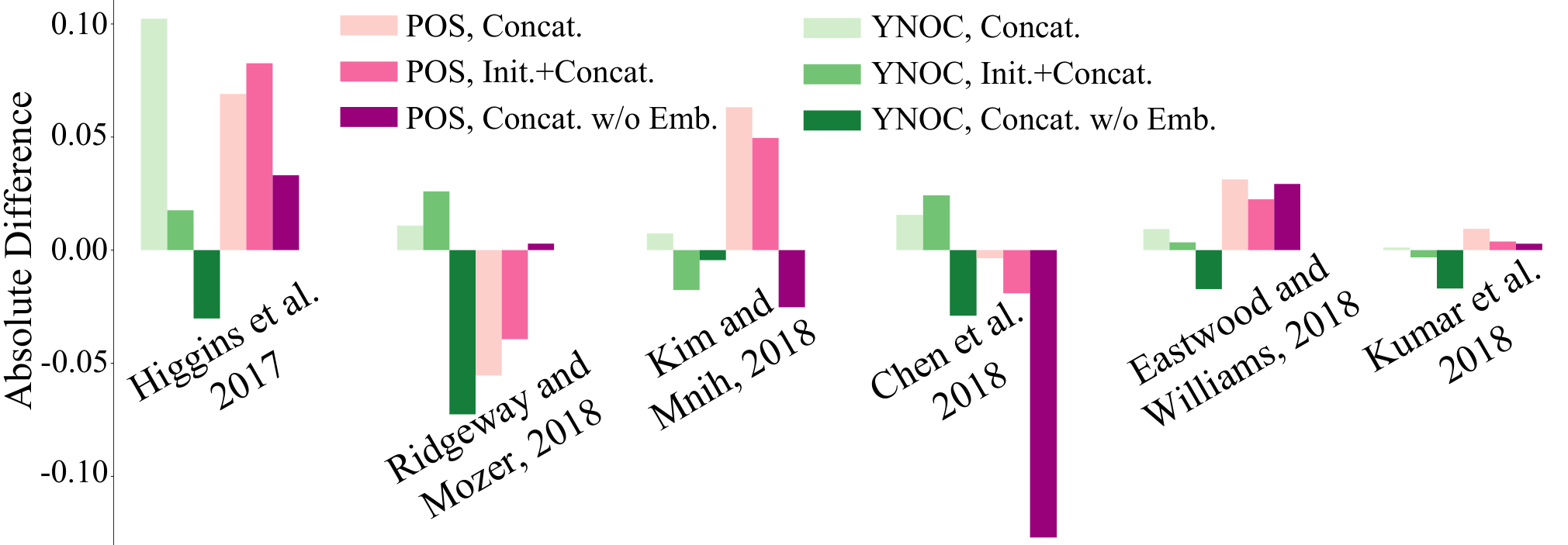
In VAEs, we typically feed the decoder with the latent code as well as word embeddings during training. The method to couple the latent code with decoder could have some effects on disentanglement for text. To highlight this, we train with 4 different coupling strategies: Init, Concat, Init Concat, Concat w/o Emb. See Figure 3(a) for an accessible visualisation. To analyse the impact of coupling, we opt for CCI-VAE which allows the comparisons to be made for the same value of KL.
We first use Concat w/o Emb to find an optimal KL in vanilla VAEs, which is then used as the to train CCI-VAEs using the other coupling metrics on YNOC and POS datasets. For YNOC, , and for POS, . This is to keep KL-divergence and reconstruction loss at the same level for fair comparison across different strategies. We report results in Table 5. Among the investigated coupling methods, the key distinguishing factor for disentanglement is their impacts on AU which is the highest for Concat.
Next, using Init as the baseline, we measure the absolute difference between disentanglement scores of different coupling methods in Figure 3(b). In general, using concatenation can bring a large improvement in disentanglement. Using both initialization and concatenation do not lead to a better result. Despite our expectation, not feeding word embeddings into decoder during training does not encourage disentanglement due to the added reliance on the latent code.
A confounding factor which could pollute this analysis is the role of strong auto-regressive decoding of VAEs and the type of information captured by the decoder in such scenario. While a preliminary analysis has been provided recently Bosc and Vincent 2020, this has been vastly under-explored and requires more explicit attempts. We leave deeper investigation of this to future work.
4.3 Disentanglement and Classification
To examine the performance of these models on real-world downstream task setting, we consider the classification task. For our classification datasets, we use DBpedia (14 classes) and Yahoo Question (10 classes) (Zhang et al. 2015). Each class of these two datasets has (10k, 1k, 1k) randomly chosen sentences in (train, dev, test) sets. We train Vanilla-VAE, -VAE (), CCI-VAE (), and MAT-VAE () from Table 3 on DBpedia and Yahoo (without the labels), then freeze the trained encoders and place a classifier on top to use the mean vector representations from the encoder as a feature to train a classifier.
We set the dimensionality of word embedding, LSTM, and the latent space to 128, 512, 32, respectively. The VAE models are trained using a batch size of 64, for 6 epochs with Adam (learning rate 0.001). For the classifier, we use a single linear layer with 1024 neurons, followed by a Softmax and train it for 15 epochs, using Adam (learning rate 0.001) and batch size 512. We illustrate the mean and standard deviation across 3 runs of models in Figure 4.
We observe that the ranking of classification accuracy among the models on DBpedia is consistent with their Top-3 performance in Table 3, with MAT-VAE outperforming the other three variants. We see roughly the same trend for Yahoo, with MAT-VAE being the dominating model. This indicates that disentangled representations are likely to be easier to discriminate, although the role of sparsely learned representations could contribute to MAT-VAE’s success as well Prokhorov et al. 2020.
4.4 Disentanglement and Generation
| Start | ||||
| , | , | |||
| ,, | , | |||
| , | , | |||
| End |
To observe the effect of disentanglement in homotopy Bowman et al. 2016, we use the exactly same toy dataset introduced in §2.1 and assess the homotopy behaviour of the highest scoring VAE vs. an ideal representation. To conduct homotopy, we interpolate between two sampled sequences’ representations and pass the intermediate representations to decoder to generate the output. We use 4D word embedding, 16D LSTM, 4D latent space. We report the results for the VAEs scoring the highest on disentanglement (w.r.t. Higgins et al. 2017 denoted as VAE-Higg) and completeness (w.r.t. Chen et al. 2018 denoted as VAE-Chen). The VAE-Higg and VAE-Chen are -VAE with and MAT-VAE with , respectively.
Additionally, to highlight the role of generative factor in generation, we conduct a dimension-wise homotopy, transitioning from the first to the last sentence by interpolating between the dimensions one-by-one. This is implemented as follows: (i) using prior distribution77 7 Instead of prior, we sample two sentences from test set and use their representations. This is to avoid the situation where samples are not in the well-estimated region of the posterior. we sample two latent codes denoted by , ; (ii) for -th dimension, using as the start, we interpolate along the -th dimension towards . Table 6 illustrates this for a 3D latent code example.
Results:
Table 7 reports the outputs for standard homotopy (top block) and dimension-wise homotopy. The results for standard homotopy demonstrate that the presence of ideally disentangled representation translates into disentangled generation in general. However, both VAE-Higg and VAE-Chen seem to mainly be producing variations of the letter in the first position (letter A) during the interpolation. The same observation holds in the dimension-wise experiments. VAE-Chen also produces variations of the letter in the second position (letter B) along with the variation of letter A, which suggests the lesser importance of completeness for disentangled representations.
| Ideal | VAE-Higg | VAE-Chen | |
| A9 B17 C13 D3 | A12 B14 C14 D12 | A9 B4 C10 D15 | |
| Homotopy | A20 B17 C1 D3 | A12 B14 C14 D12 | A7 B4 C10 D15 |
| A4 B17 C12 D6 | A8 B14 C14 D12 | A14 B4 C10 D15 | |
| A3 B1 C6 D6 | A20 B14 C14 D12 | A20 B19 C10 D15 | |
| A13 B1 C6 D20 | A15 B14 C14 D12 | A8 B19 C10 D15 | |
| A15 B2 C8 D10 | A4 B14 C14 D12 | A12 B19 C10 D15 | |
| A9 B17 C13 D3 | A12 B14 C14 D12 | A9 B4 C10 D15 | |
| Dim 1 | A20 B17 C13 D3 | A12 B14 C14 D12 | A7 B4 C10 D15 |
| A4 B17 C13 D3 | A8 B14 C14 D12 | A4 B19 C10 D15 | |
| A3 B17 C13 D3 | A20 B14 C14 D12 | A8 B19 C10 D15 | |
| A13 B17 C13 D3 | A18 B14 C14 D12 | A12 B19 C10 D15 | |
| A15 B17 C13 D3 | A4 B14 C14 D12 | A12 B19 C10 D15 | |
| Dim 2 | A15 B17 C13 D3 | A4 B14 C14 D12 | A12 B19 C10 D15 |
| A15 B17 C13 D3 | A4 B14 C14 D12 | A12 B19 C10 D15 | |
| A15 B17 C13 D3 | A4 B14 C14 D12 | A12 B19 C10 D15 | |
| A15 B1 C13 D3 | A4 B14 C14 D12 | A12 B19 C10 D15 | |
| A15 B2 C13 D3 | A4 B14 C14 D12 | A12 B19 C10 D15 | |
| Dim 3 | A15 B2 C1 D3 | A4 B14 C14 D12 | A12 B19 C10 D15 |
| A15 B2 C12 D3 | A4 B14 C14 D12 | A12 B19 C10 D15 | |
| A15 B2 C6 D3 | A4 B14 C14 D12 | A12 B19 C10 D15 | |
| A15 B2 C6 D3 | A4 B14 C14 D12 | A12 B19 C10 D15 | |
| A15 B2 C8 D3 | A4 B14 C14 D12 | A12 B19 C10 D15 | |
| Dim 4 | A15 B2 C8 D3 | A4 B14 C14 D12 | A12 B19 C10 D15 |
| A15 B2 C8 D6 | A4 B14 C14 D12 | A12 B19 C10 D15 | |
| A15 B2 C8 D6 | A4 B14 C14 D12 | A12 B19 C10 D15 | |
| A15 B2 C8 D20 | A4 B14 C14 D12 | A12 B19 C10 D15 | |
| A15 B2 C8 D10 | A4 B14 C14 D12 | A12 B19 C10 D15 |
This indicates that despite the relative superior performance of certain models on the metrics and classification tasks, the amount of disentanglement present in the representation is not sufficient enough to be reflected by the generative behavior of these models. As a future work, we would look into the role of auto-regressive decoding and teacher-forcing as confounding factors that can potentially affect the disentanglement process.
5 Conclusion and Future Directions
We evaluated a set of recent unsupervised disentanglement learning frameworks widely used in image domain on two artificially created corpora with known underlying generative factors. Our experiments highlight the existing gaps in text domain, the daunting tasks state-of-the-art models from image domain face on text, and the confounding elements that pose further challenges towards representation disentanglement in text domain. Motivated by our findings, in future, we will explore the role of inductive biases such as representation sparsity in achieving representation disentanglement. Additionally, we will look into alternative forms of decoding and training which may compromise reconstruction quality but increase the reliance of decoding on the representation, hence allowing for a more controlled analysis and evaluation.
Our synthetic datasets and experimental framework provide a set of quantitative and qualitative measures to facilitate and future research in developing new models, datasets, and evaluation metrics specific for text.
References
- Alemi et al. (2018) Alexander Alemi, Ben Poole, Ian Fischer, Joshua Dillon, Rif A Saurous, and Kevin Murphy. 2018. Fixing a broken elbo. In International Conference on Machine Learning, pages 159–168. PMLR.
- Balasubramanian et al. (2021) Vikash Balasubramanian, Ivan Kobyzev, Hareesh Bahuleyan, Ilya Shapiro, and Olga Vechtomova. 2021. Polarized-VAE: Proximity based disentangled representation learning for text generation. In Proceedings of the 16th Conference of the European Chapter of the Association for Computational Linguistics: Main Volume, pages 416–423, Online. Association for Computational Linguistics.
- Bao et al. (2019) Yu Bao, Hao Zhou, Shujian Huang, Lei Li, Lili Mou, Olga Vechtomova, Xin-yu Dai, and Jiajun Chen. 2019. Generating sentences from disentangled syntactic and semantic spaces. In Proceedings of the 57th Annual Meeting of the Association for Computational Linguistics, pages 6008–6019, Florence, Italy. Association for Computational Linguistics.
- Bengio et al. (2013) Y. Bengio, A. Courville, and P. Vincent. 2013. Representation learning: A review and new perspectives. IEEE Transactions on Pattern Analysis and Machine Intelligence, 35(8):1798–1828.
- Bengio (2013) Yoshua Bengio. 2013. Deep learning of representations: Looking forward. In Statistical Language and Speech Processing - First International Conference, SLSP 2013, Tarragona, Spain, July 29-31, 2013. Proceedings, volume 7978 of Lecture Notes in Computer Science, pages 1–37. Springer.
- Bosc and Vincent (2020) Tom Bosc and Pascal Vincent. 2020. Do sequence-to-sequence VAEs learn global features of sentences? In Proceedings of the 2020 Conference on Empirical Methods in Natural Language Processing (EMNLP), pages 4296–4318, Online. Association for Computational Linguistics.
- Bowman et al. (2016) Samuel R. Bowman, Luke Vilnis, Oriol Vinyals, Andrew M. Dai, Rafal Józefowicz, and Samy Bengio. 2016. Generating sentences from a continuous space. In Proceedings of the 20th SIGNLL Conference on Computational Natural Language Learning, CoNLL 2016, pages 10–21, Berlin, Germany. ACL.
- Burgess et al. (2018) Christopher P. Burgess, Irina Higgins, Arka Pal, Loïc Matthey, Nick Watters, Guillaume Desjardins, and Alexander Lerchner. 2018. Understanding disentangling in -vae. CoRR, abs/1804.03599.
- Chen et al. (2019) Mingda Chen, Qingming Tang, Sam Wiseman, and Kevin Gimpel. 2019. A multi-task approach for disentangling syntax and semantics in sentence representations. In Proceedings of the 2019 Conference of the North American Chapter of the Association for Computational Linguistics: Human Language Technologies, Volume 1 (Long and Short Papers), pages 2453–2464, Minneapolis, Minnesota. Association for Computational Linguistics.
- Chen et al. (2018) Ricky T. Q. Chen, Xuechen Li, Roger B Grosse, and David K Duvenaud. 2018. Isolating sources of disentanglement in variational autoencoders. In Advances in Neural Information Processing Systems, volume 31, pages 2610–2620. Curran Associates, Inc.
- Cheng et al. (2020) Pengyu Cheng, Martin Renqiang Min, Dinghan Shen, Christopher Malon, Yizhe Zhang, Yitong Li, and Lawrence Carin. 2020. Improving disentangled text representation learning with information-theoretic guidance. In Proceedings of the 58th Annual Meeting of the Association for Computational Linguistics, pages 7530–7541, Online. Association for Computational Linguistics.
- Conneau et al. (2018) Alexis Conneau, German Kruszewski, Guillaume Lample, Loïc Barrault, and Marco Baroni. 2018. What you can cram into a single $&!#* vector: Probing sentence embeddings for linguistic properties. In Proceedings of the 56th Annual Meeting of the Association for Computational Linguistics (Volume 1: Long Papers), pages 2126–2136, Melbourne, Australia. Association for Computational Linguistics.
- Dieng et al. (2019) Adji B. Dieng, Yoon Kim, Alexander M. Rush, and David M. Blei. 2019. Avoiding latent variable collapse with generative skip models. In The 22nd International Conference on Artificial Intelligence and Statistics, AISTATS 2019, volume 89 of Proceedings of Machine Learning Research, pages 2397–2405, Naha, Okinawa, Japan. PMLR.
- Dittadi et al. (2021) Andrea Dittadi, Frederik Träuble, Francesco Locatello, Manuel Wuthrich, Vaibhav Agrawal, Ole Winther, Stefan Bauer, and Bernhard Schölkopf. 2021. On the transfer of disentangled representations in realistic settings. In International Conference on Learning Representations.
- Eastwood and Williams (2018) Cian Eastwood and Christopher K. I. Williams. 2018. A framework for the quantitative evaluation of disentangled representations. In International Conference on Learning Representations.
- Ettinger et al. (2018) Allyson Ettinger, Ahmed Elgohary, Colin Phillips, and Philip Resnik. 2018. Assessing composition in sentence vector representations. In Proceedings of the 27th International Conference on Computational Linguistics, pages 1790–1801, Santa Fe, New Mexico, USA. Association for Computational Linguistics.
- Gretton et al. (2012) Arthur Gretton, Karsten M. Borgwardt, Malte J. Rasch, Bernhard Schölkopf, and Alexander Smola. 2012. A kernel two-sample test. Journal of Machine Learning Research, 13(25):723–773.
- He et al. (2019) Junxian He, Daniel Spokoyny, Graham Neubig, and Taylor Berg-Kirkpatrick. 2019. Lagging inference networks and posterior collapse in variational autoencoders. In 7th International Conference on Learning Representations, ICLR 2019, New Orleans, LA, USA.
- Hewitt and Liang (2019) John Hewitt and Percy Liang. 2019. Designing and interpreting probes with control tasks. In Proceedings of the 2019 Conference on Empirical Methods in Natural Language Processing and the 9th International Joint Conference on Natural Language Processing (EMNLP-IJCNLP), pages 2733–2743, Hong Kong, China. Association for Computational Linguistics.
- Higgins et al. (2018) Irina Higgins, David Amos, David Pfau, Sébastien Racanière, Loïc Matthey, Danilo J. Rezende, and Alexander Lerchner. 2018. Towards a definition of disentangled representations. CoRR, abs/1812.02230.
- Higgins et al. (2017) Irina Higgins, Loïc Matthey, Arka Pal, Christopher Burgess, Xavier Glorot, Matthew Botvinick, Shakir Mohamed, and Alexander Lerchner. 2017. beta-vae: Learning basic visual concepts with a constrained variational framework. In 5th International Conference on Learning Representations, ICLR 2017, Conference Track Proceedings, Toulon, France.
- Hurley and Rickard (2009) N. Hurley and S. Rickard. 2009. Comparing measures of sparsity. IEEE Transactions on Information Theory, 55(10):4723–4741.
- John et al. (2019) Vineet John, Lili Mou, Hareesh Bahuleyan, and Olga Vechtomova. 2019. Disentangled representation learning for non-parallel text style transfer. In Proceedings of the 57th Annual Meeting of the Association for Computational Linguistics, pages 424–434, Florence, Italy. Association for Computational Linguistics.
- Kim and Mnih (2018) Hyunjik Kim and Andriy Mnih. 2018. Disentangling by factorising. In Proceedings of the 35th International Conference on Machine Learning, ICML 2018, volume 80 of Proceedings of Machine Learning Research, pages 2649–2658, Stockholmsmässan, Stockholm Sweden. PMLR.
- Kingma and Ba (2015) Diederik P. Kingma and Jimmy Ba. 2015. Adam: A method for stochastic optimization. In 3rd International Conference on Learning Representations, ICLR 2015, Conference Track Proceedings, San Diego, CA, USA.
- Kingma and Welling (2014) Diederik P. Kingma and Max Welling. 2014. Auto-encoding variational bayes. In 2nd International Conference on Learning Representations, ICLR 2014, Banff, AB, Canada, April 14-16, 2014, Conference Track Proceedings.
- Kumar et al. (2018) Abhishek Kumar, Prasanna Sattigeri, and Avinash Balakrishnan. 2018. VARIATIONAL INFERENCE OF DISENTANGLED LATENT CONCEPTS FROM UNLABELED OBSERVATIONS. In International Conference on Learning Representations.
- Locatello et al. (2019) Francesco Locatello, Stefan Bauer, Mario Lucic, Gunnar Raetsch, Sylvain Gelly, Bernhard Schölkopf, and Olivier Bachem. 2019. Challenging common assumptions in the unsupervised learning of disentangled representations. In Proceedings of the 36th International Conference on Machine Learning, ICML 2019, volume 97 of Proceedings of Machine Learning Research, pages 4114–4124, Long Beach, California, USA. PMLR.
- Marvin and Linzen (2018) Rebecca Marvin and Tal Linzen. 2018. Targeted syntactic evaluation of language models. In Proceedings of the 2018 Conference on Empirical Methods in Natural Language Processing, pages 1192–1202, Brussels, Belgium. Association for Computational Linguistics.
- Mathieu et al. (2019) Emile Mathieu, Tom Rainforth, N Siddharth, and Yee Whye Teh. 2019. Disentangling disentanglement in variational autoencoders. In Proceedings of the 36th International Conference on Machine Learning, volume 97 of Proceedings of Machine Learning Research, pages 4402–4412. PMLR.
- Mitchell and Beauchamp (1988) T. J. Mitchell and J. J. Beauchamp. 1988. Bayesian variable selection in linear regression. Journal of the American Statistical Association, 83(404):1023–1032.
- Montero et al. (2021) Milton Llera Montero, Casimir JH Ludwig, Rui Ponte Costa, Gaurav Malhotra, and Jeffrey Bowers. 2021. The role of disentanglement in generalisation. In International Conference on Learning Representations.
- Pelsmaeker and Aziz (2020) Tom Pelsmaeker and Wilker Aziz. 2020. Effective estimation of deep generative language models. In Proceedings of the 58th Annual Meeting of the Association for Computational Linguistics, pages 7220–7236, Online. Association for Computational Linguistics.
- Pimentel et al. (2020) Tiago Pimentel, Josef Valvoda, Rowan Hall Maudslay, Ran Zmigrod, Adina Williams, and Ryan Cotterell. 2020. Information-theoretic probing for linguistic structure. In Proceedings of the 58th Annual Meeting of the Association for Computational Linguistics, pages 4609–4622, Online. Association for Computational Linguistics.
- Prokhorov et al. (2020) Victor Prokhorov, Yingzhen Li, Ehsan Shareghi, and Nigel Collier. 2020. Hierarchical sparse variational autoencoder for text encoding. arXiv preprint arXiv:2009.12421.
- Prokhorov et al. (2019) Victor Prokhorov, Ehsan Shareghi, Yingzhen Li, Mohammad Taher Pilehvar, and Nigel Collier. 2019. On the importance of the Kullback-Leibler divergence term in variational autoencoders for text generation. In Proceedings of the 3rd Workshop on Neural Generation and Translation, pages 118–127, Hong Kong. Association for Computational Linguistics.
- Razavi et al. (2019) Ali Razavi, Aäron van den Oord, Ben Poole, and Oriol Vinyals. 2019. Preventing posterior collapse with delta-vaes. In 7th International Conference on Learning Representations, ICLR 2019, New Orleans, LA, USA.
- Ridgeway and Mozer (2018) Karl Ridgeway and Michael C Mozer. 2018. Learning deep disentangled embeddings with the f-statistic loss. In Advances in Neural Information Processing Systems, volume 31, pages 185–194. Curran Associates, Inc.
- Ross and Doshi-Velez (2021) Andrew Slavin Ross and Finale Doshi-Velez. 2021. Benchmarks, algorithms, and metrics for hierarchical disentanglement. CoRR, abs/2102.05185.
- Torroba Hennigen et al. (2020) Lucas Torroba Hennigen, Adina Williams, and Ryan Cotterell. 2020. Intrinsic probing through dimension selection. In Proceedings of the 2020 Conference on Empirical Methods in Natural Language Processing (EMNLP), pages 197–216, Online. Association for Computational Linguistics.
- Voita and Titov (2020) Elena Voita and Ivan Titov. 2020. Information-theoretic probing with minimum description length. In Proceedings of the 2020 Conference on Empirical Methods in Natural Language Processing (EMNLP), pages 183–196, Online. Association for Computational Linguistics.
- Yang et al. (2017) Zichao Yang, Zhiting Hu, Ruslan Salakhutdinov, and Taylor Berg-Kirkpatrick. 2017. Improved variational autoencoders for text modeling using dilated convolutions. In Proceedings of the 34th International Conference on Machine Learning, ICML 2017, volume 70 of Proceedings of Machine Learning Research, pages 3881–3890, Sydney, NSW, Australia. PMLR.
- Zhang et al. (2015) Xiang Zhang, Junbo Zhao, and Yann LeCun. 2015. Character-level convolutional networks for text classification. In Proceedings of the 28th International Conference on Neural Information Processing Systems - Volume 1, NIPS’15, page 649–657, Cambridge, MA, USA. MIT Press.
Appendix A Disentanglement Metrics Algorithms
To evaluate representations learned by a model on a dataset having the attributes of Data Requirement, we further require a series of representation space , who has a bijection mapping with . Hence, when sampling representations which have the same value on one generative factor, we only need to sample in one .
Under these notations, we write the pseudo code of metrics in Algorithm 1-6. For Algorithm 5 and 6, although we only use one criterion in the main paper, we still provide the details for other criteria. We set and for Algorithm 1 and 2, and for Algorithm 3, 4, 5, and 6.
Modularity:
Explicitness: