跳到论文正文
W Papers独立论文阅读器 arXiv:2106.03510 论文正文 计算阅读时间 · 0%
引用这篇论文根据当前论文元数据生成,正式投稿前建议核对。


License: CC BY 4.0
arXiv:2106.03510v2 [math.PR] 15 Jul 2022

Cooling down stochastic differential equations:
almost sure convergence

Steffen Dereich Address: Steffen Dereich
Institut für Mathematische Stochastik
Fachbereich 10: Mathematik und Informatik
Westfälische Wilhelms-Universität Münster
Orléans-Ring 10
48149 Münster
Germany
Email address: steffen.dereich@wwu.de
and Sebastian Kassing Address: Sebastian Kassing
Institut für Mathematische Stochastik
Fachbereich 10: Mathematik und Informatik
Westfälische Wilhelms-Universität Münster
Orléans-Ring 10
48149 Münster
Germany
Email address: sebastian.kassing@wwu.de
Abstract.

We consider almost sure convergence of the SDE d​Xt=αt​d​t+βt​d​WtdX_{t}=\alpha_{t}\,dt+\beta_{t}\,dW_{t} under the existence of a C2C^{2}-Lyapunov function F:ℝd→ℝF:{\mathbb{R}}^{d}\to{\mathbb{R}}. More explicitly, we show that on the event that the process stays local we have almost sure convergence in the Lyapunov function (F⁡(Xt))t≥0(F(X_{t}))_{t\geq 0} as well as ∇F​(Xt)→0\nabla F(X_{t})\to 0, if |βt|=𝒪⁡(t−β)|\beta_{t}|=\mathcal{O}(t^{-\beta}) for a β>1/2\beta>1/2. If, additionally, one assumes that FF is a Łojasiewicz-function, we get almost sure convergence of the process itself, given that |βt|=𝒪⁡(t−β)|\beta_{t}|=\mathcal{O}(t^{-\beta}) for a β>1\beta>1. The assumptions are shown to be optimal in the sense that there is a divergent counterexample where |βt||\beta_{t}| is of order t−1t^{-1}.

Key words and phrases: 
Stochastic gradient flow; Brownian particle; cooling down; Łojasiewicz-inequality; almost sure convergence
2020 Mathematics Subject Classification
Primary 60J60; Secondary 60H10, 65C35

1. Introduction

Let (Ω,(ℱt)t≥0,ℱ,ℙ)(\Omega,(\mathcal{F}_{t})_{t\geq 0},\mathcal{F},{\mathbb{P}}) be a filtered probability space satisfying the usual conditions and suppose that (Xt)t≥0(X_{t})_{t\geq 0} is a continuous semimartingale satisfying the equation

(1) Xt−X0=∫0tαs​𝑑s+∫0tβs​d​Ws,\displaystyle X_{t}-X_{0}=\int_{0}^{t}\alpha_{s}\,ds+\int_{0}^{t}\beta_{s}\,dW_{s},

for all t≥0t\geq 0, where

  • •

    (αt)t≥0(\alpha_{t})_{t\geq 0} is a progressive, ℝd{\mathbb{R}}^{d}-valued process,

  • •

    (βt)t≥0(\beta_{t})_{t\geq 0} is a progressive ℝd×d′{\mathbb{R}}^{d\times d^{\prime}}-valued process and

  • •

    (Wt)t≥0(W_{t})_{t\geq 0} is an ℝd′{\mathbb{R}}^{d^{\prime}}-valued (ℱt)t≥0(\mathcal{F}_{t})_{t\geq 0}-Brownian motion with initial value W0=0W_{0}=0.

In this article, we analyse convergence of (Xt)t≥0(X_{t})_{t\geq 0} under the assumption that the drift term satisfies a Lyapunov kind of condition and the diffusivity converges to zero sufficiently fast. More explicitly, we denote by F:ℝd→ℝF:{\mathbb{R}}^{d}\to{\mathbb{R}} a C2C^{2}-function, by f:=∇Ff:=\nabla F its gradient and by H:=Hess​FH:=\text{Hess}\,F the Hessian of FF and consider the following event

ℂ:={lim inft→∞\displaystyle{\mathbb{C}}:=\Bigl\{\liminf_{t\to\infty} ⟨f⁡(Xt),−αt⟩|f⁡(Xt)|2>0,lim inft→∞|f⁡(Xt)||αt|>0,\displaystyle\frac{\langle f(X_{t}),-\alpha_{t}\rangle}{|f(X_{t})|^{2}}>0,\,\liminf_{t\to\infty}\frac{|f(X_{t})|}{|\alpha_{t}|}>0,
∫0∞|βs|F2ds<∞ andlim supt→∞|βt|<∞},\displaystyle\quad\int_{0}^{\infty}|\beta_{s}|_{F}^{2}\,ds<\infty\,\text{ and}\ \limsup\limits_{t\to\infty}|\beta_{t}|<\infty\Bigr\},

where we interpret 00\frac{0}{0} as ∞\infty and, for a matrix A∈ℝd×d′A\in{\mathbb{R}}^{d\times d^{\prime}}, |A|F|A|_{F} (resp. |A||A|) denotes the Frobenius norm (resp. spectral norm). Intuitively, on ℂ{\mathbb{C}} the drift term (αt)t≥0(\alpha_{t})_{t\geq 0} is comparable in size and direction to the negative gradient of the Lyapunov function, i.e., (−∇F​(Xt))t≥0(-\nabla F(X_{t}))_{t\geq 0}, and the size of the diffusivity (βt)t≥0(\beta_{t})_{t\geq 0} can be controlled at late times. The first and second condition in the definition of the event ℂ{\mathbb{C}} are obviously satisfied if we consider the solution to the SDE

(2) d​Xt=−∇F​(Xt)​d​t+βt​d​Wt,\displaystyle dX_{t}=-\nabla F(X_{t})\,dt+\beta_{t}\,dW_{t},

which represents the canonical stochastic version of the gradient flow ODE

x˙t=−∇F​(xt).\dot{x}_{t}=-\nabla F(x_{t}).

However, the current framework allows more flexibility in the drift term. We will restrict attention to certain events: set

𝔹:={lim inft→∞F(Xt)>−∞,lim supt→∞|αt|<∞ and lim supε→0lim supt→∞y∈B⁡(Xt,ε)|H(y)|<∞}\mathbb{B}:=\Biggl\{\liminf_{t\to\infty}F(X_{t})>-\infty,\,\limsup_{t\to\infty}|\alpha_{t}|<\infty\text{ and }\limsup_{\varepsilon\to 0}\limsup_{\begin{subarray}{c}t\to\infty\\ y\in B(X_{t},\varepsilon)\end{subarray}}|H(y)|<\infty\Biggr\}

and

𝕃:={lim supt→∞|Xt|<∞}.{\mathbb{L}}:=\Bigl\{\limsup_{t\to\infty}|X_{t}|<\infty\Bigr\}.

We separately show almost sure convergence of (F⁡(Xt))t≥0,(f⁡(Xt))t≥0(F(X_{t}))_{t\geq 0},(f(X_{t}))_{t\geq 0} and (Xt)t≥0(X_{t})_{t\geq 0} under mild assumptions on the diffusivity and the underlying Lyapunov function which are shown to be optimal (c.f. Chapter 4). The SDE (2) is the continuous-time counterpart for the stochastic gradient descent scheme (when (βt)t≥0(\beta_{t})_{t\geq 0} is chosen properly, see [LTE17]) and, thus, a helpful tool for gaining intuition and insight on the behaviour of SGD. It also appears naturally in applications from Physics and Chemistry. For example, (2) can be viewed as the pathwise solution to the Fokker–Planck equation (see [Gar85]) in a physical system, where FF models the energy and (βt)t≥0(\beta_{t})_{t\geq 0} an external source of perturbation11 1 (2/βt2)t≥0(2/\beta_{t}^{2})_{t\geq 0} is sometimes referred to as the inverse temperature, e.g. [CHS87, JKO98], or as the chemical Langevin equation describing a chemical reaction evolving in time ([vK92], [Gil00], [SSG14]). In our analysis, we allow general non-convex energy landscapes and focus on the case where the perturbation fades within time.

There are several asymptotic results for the solution (Xt)t≥0(X_{t})_{t\geq 0} of (2) when choosing a deterministic diffusivity (βt)t≥0(\beta_{t})_{t\geq 0}. Inspired by simulated annealing, [GH86] and [CHS87] proved that for (βt)t≥0=(2​c/log⁡(t+1))t≥0(\beta_{t})_{t\geq 0}=(\sqrt{2c/\log(t+1)})_{t\geq 0} with sufficiently large c>0c>0 and under additional assumptions on the target function FF, the solution of (2) converges weakly to a distribution π\pi concentrated on the global minima of FF independent of the initial value X0=x∈ℝdX_{0}=x\in{\mathbb{R}}^{d}, even in the case of non-convex target functions FF. More precisely, π\pi is the weak limit of the Gibbs densities πt(x)∝exp(−2F(x)/βt2)\pi_{t}(x)\propto\exp(-2F(x)/\beta^{2}_{t}). In this regime, [HKS89] showed that if the diffusion process is defined on a compact manifold, then (F⁡(Xt))t≥0(F(X_{t}))_{t\geq 0} converges to the optimal value in probability if and only if c>c∗c>c^{*}, where c∗c^{*} denotes the minimal potential energy necessary to connect every point with a global minimum using a continuous path. Recently, this result has been generalised by [FT21] to diffusions on ℝd{\mathbb{R}}^{d} in the case where F∈C∞F\in C^{\infty} is assumed to satisfy lim|x|→∞F⁡(x)=∞\lim_{|x|\to\infty}F(x)=\infty and ∫ℝde−α0​F​(x)​𝑑x<∞\int_{{\mathbb{R}}^{d}}e^{-\alpha_{0}F(x)}\,dx<\infty for some α0>0\alpha_{0}>0. In that case one has lim inft→∞|Xt|<∞\liminf_{t\to\infty}|X_{t}|<\infty, almost surely.

However, in this particular scenario we cannot hope for the individual paths of the solution (Xt)t≥0(X_{t})_{t\geq 0} to converge. Conversely, the diffusivity (βt)t≥0(\beta_{t})_{t\geq 0} considered here converges significantly faster to zero. Therefore, we cannot guarantee that the process (Xt)t≥0(X_{t})_{t\geq 0} started in the basin of attraction of a bad local minimum is able to overcome a barrier in the landscape in order to converge to a global minimum (see Section 3.3) and the distribution of the limit points of (Xt)t≥0(X_{t})_{t\geq 0} depends heavily on the distribution of the initial value X0X_{0}. As we will indicate below, the gradient flow converges if FF is a Łojasiewicz-landscape, in the sense of Definition 1.4, and the gradient flow does not escape to infinity. The main contribution of this article is the analysis in how far this is still the case when additionally incorporating a stochastic perturbation. We stress that we analyse the asymptotic behaviour of the system as time tends to infinite which is significantly different from the analysis of families of SDEs where the diffusivity decays with a family index ε>0\varepsilon>0, see e.g. [FW12].

First, we will provide a short proof for almost sure convergence of (F⁡(Xt))t≥0(F(X_{t}))_{t\geq 0} and (f⁡(Xt))t≥0(f(X_{t}))_{t\geq 0} with limt→∞f⁡(Xt)=0\lim_{t\to\infty}f(X_{t})=0 on the event ℂ∩𝔹{\mathbb{C}}\cap\mathbb{B}. We conclude that we have a.s. convergence of (Xt)t≥0(X_{t})_{t\geq 0} on the event ℂ∩𝕃{\mathbb{C}}\cap{\mathbb{L}} in the case where where the set of critical points 𝒞:={x∈ℝd:f⁡(x)=0}\mathcal{C}:=\{x\in{\mathbb{R}}^{d}:f(x)=0\} is at most countable.

Theorem 1.1.

On ℂ∩𝔹{\mathbb{C}}\cap\mathbb{B}, almost surely, (F⁡(Xt))t≥0(F(X_{t}))_{t\geq 0} converges to a finite value and limt→∞f⁡(Xt)=0\lim_{t\to\infty}f(X_{t})=0 as well as lim supt0→∞∫t0∞⟨f⁡(Xs),−αs⟩​𝑑s<∞\limsup_{t_{0}\to\infty}\int_{t_{0}}^{\infty}\langle f(X_{s}),-\alpha_{s}\rangle\,ds<\infty. If the set of critical points of FF is at most countable, then, on ℂ∩𝕃{\mathbb{C}}\cap{\mathbb{L}}, almost surely, (Xt)t≥0(X_{t})_{t\geq 0} converges.

Theorem 1.1 is an immediate consequence of the more general Proposition 2.1 below.

Remark 1.2.

Note that as FF is C2C^{2} we clearly have ℂ∩𝕃⊂ℂ∩𝔹{\mathbb{C}}\cap{\mathbb{L}}\subset{\mathbb{C}}\cap\mathbb{B} so that the first statement of Theorem 1.1 also holds on ℂ∩𝕃{\mathbb{C}}\cap{\mathbb{L}}. Moreover, for a Lyapunov function FF with lim inf|x|→∞|f⁡(x)|>0\liminf_{|x|\to\infty}|f(x)|>0 the first statement implies that

ℂ∩𝔹=ℂ∩𝕃.{\mathbb{C}}\cap\mathbb{B}={\mathbb{C}}\cap{\mathbb{L}}.
Remark 1.3.

A standard approach for proving convergence statements similar to those given in Theorem 1.1 is the theory of asymptotic pseudotrajectories (see [Ben99], especially Corollary 6.7). While these methods may lead to different and typically weaker assumptions on the perturbation (βt)t≥0(\beta_{t})_{t\geq 0}, Theorem 1.1 will mainly be used to prove Theorem 1.6 below. In order to be self-contained we stated Theorem 1.1 in such a way that it can easily be applied in Theorem 1.6 and has a direct and brief proof.

In the case where the set of critical points of FF contains a continuum of elements the situation is more subtle. Even in the case without random perturbations convergence of the solution (xt)t≥0(x_{t})_{t\geq 0} to the ODE

(3) x˙t=−∇F​(xt)\displaystyle\dot{x}_{t}=-\nabla F(x_{t})

is a non-trivial issue: one can find C∞C^{\infty}-functions FF together with solutions (xt)t≥0(x_{t})_{t\geq 0} that stay on compact sets but do not converge, see example 3 on page 14 of [PdM82]. Counterexamples of this structure have been known for a long time (see e.g. [Cur44]) and include the famous Mexican hat function [AMA05]. To guarantee convergence (at least in the case where the solution stays on a compact set), one needs to impose additional assumptions. An appropriate assumption is the validity of a Łojasiewicz-inequality, see Definition 1.4 below. This assumption has the appeal that it is satisfied by analytic functions, see [Łoj63, Łoj65]. With the help of the inequality (4) Łojasiewicz showed in [Łoj84] that any integral curve of the gradient flow equation (3) for an analytic function FF that has an accumulation point has a unique limit. A proof of that assertion can also be found in [Har12] or [CMI14].

In this article, we device a probabilistic counterpart to the classical analytic approach. We will derive moment estimates of F⁡(Xt)F(X_{t}) for Łojasiewicz-functions F:ℝd→ℝF:{\mathbb{R}}^{d}\to{\mathbb{R}} on ℂ∩𝕃{\mathbb{C}}\cap{\mathbb{L}} under the additional assumption that we can asymptotically bound the diffusivity (βt)t≥0(\beta_{t})_{t\geq 0} by a locally-bounded deterministic function σ:[0,∞)→[0,∞)\sigma:[0,\infty)\to[0,\infty) to deduce almost sure convergence of (∫0tαs​𝑑s)t≥0(\int_{0}^{t}\alpha_{s}\,ds)_{t\geq 0} and thus, almost sure convergence of (Xt)t≥0(X_{t})_{t\geq 0}.

Definition 1.4.

We call the function F:ℝd→ℝF:{\mathbb{R}}^{d}\to{\mathbb{R}} Łojasiewicz-function, if for every x∈𝒞:=f−1​({0})x\in\mathcal{C}:=f^{-1}(\{0\}), the Łojasiewicz-inequality is true on a neighbourhood UxU_{x} of xx with parameters Ł>0\L>0 and θ∈[12,1)\theta\in[\frac{1}{2},1), i.e., for all y∈Uxy\in U_{x}

(4) |f⁡(y)|≥Ł​|F⁡(y)−F⁡(x)|θ.\displaystyle|f(y)|\geq\L\,|F(y)-F(x)|^{\theta}.
Remark 1.5.

Note that for all x∉𝒞x\notin\mathcal{C} and θ∈[12,1)\theta\in[\frac{1}{2},1) there trivially exist a neighbourhood UxU_{x} and constant Ł>0\L>0 such that the Łojasiewicz-inequality with parameter Ł\L and θ\theta hold on UxU_{x}.

The main contribution of this article concerns convergence of the SDE in the case where the Lyapunov function is a Łojasiewicz-function.

Theorem 1.6.

Let FF be a Łojasiewicz-function and (σt)t≥0=((t+1)−σ)t≥0(\sigma_{t})_{t\geq 0}=((t+1)^{-\sigma})_{t\geq 0} with σ>1\sigma>1. Then, on ℂ∩𝕃∩{lim supt→∞|βt|σt<∞}{\mathbb{C}}\cap{\mathbb{L}}\cap\bigl\{\limsup_{t\to\infty}\frac{|\beta_{t}|}{\sigma_{t}}<\infty\bigr\}, the process (Xt)t≥0(X_{t})_{t\geq 0} satisfying (1) converges, almost surely, to a critical point of FF.

The proof of the theorem is accomplished in Section 3. The theorem is optimal in the sense that its conclusion is not true for the choice (σt)t≥0=((t+1)−1)t≥0(\sigma_{t})_{t\geq 0}=((t+1)^{-1})_{t\geq 0}. More explicitly, we provide an SDE for which ℂ∩𝕃∩{lim supt→∞(t+1)|βt|<∞}{\mathbb{C}}\cap{\mathbb{L}}\cap\bigl\{\limsup_{t\to\infty}(t+1)|\beta_{t}|<\infty\bigr\} is an almost sure set and for which (Xt)t≥0(X_{t})_{t\geq 0} diverges, almost surely, in Section 4.

Remark 1.7.

Choose (αt)t≥0=(−f⁡(Xt))t≥0(\alpha_{t})_{t\geq 0}=(-f(X_{t}))_{t\geq 0} and consider the solution to the SDE (2). In that case we have for (σt)t≥0(\sigma_{t})_{t\geq 0} as in Theorem 1.6 that {lim supt→∞|βt|σt<∞}⊂ℂ.\bigl\{\limsup_{t\to\infty}\frac{|\beta_{t}|}{\sigma_{t}}<\infty\bigr\}\subset{\mathbb{C}}. Now, assume that F∈C2F\in C^{2} satisfies lim|x|→∞F⁡(x)=∞\lim_{|x|\to\infty}F(x)=\infty. In Appendix A we derive sufficient conditions that guarantee locality of the process (Xt)t≥0(X_{t})_{t\geq 0}. In particular, we show that if the Hessian of FF is uniformly bounded (i.e. supx∈ℝd|H⁡(x)|<∞\sup_{x\in{\mathbb{R}}^{d}}|H(x)|<\infty) then {∫0∞|βs|F2ds<∞}⊂𝕃\bigl\{\int_{0}^{\infty}|\beta_{s}|_{F}^{2}\,ds<\infty\bigr\}\subset{\mathbb{L}}. Also, we get for any compact set K⊂ℝdK\subset{\mathbb{R}}^{d}

{\displaystyle\Bigl\{ 1l{Xt∉K}(−|f(Xt)|2+12tr((βt)†H(Xt)βt))≤0 for all large t\displaystyle 1\hskip-2.78857pt\mathrm{l}_{\{X_{t}\notin K\}}(-|f(X_{t})|^{2}+\frac{1}{2}\mathrm{tr}((\beta_{t})^{\dagger}H(X_{t})\beta_{t}))\leq 0\text{ for all large }t
and ∫0∞1l{Xs∈K}|βs|F2ds<∞}⊂𝕃.\displaystyle\text{ and }\int_{0}^{\infty}1\hskip-2.78857pt\mathrm{l}_{\{X_{s}\in K\}}|\beta_{s}|_{F}^{2}\,ds<\infty\Bigr\}\subset{\mathbb{L}}.

The proof of Theorem 1.6 is based on moment estimates for F⁡(Xt)F(X_{t}) restricted to particular events, see Proposition 3.1 below. In the particular case where we approach a local minimum these estimates entail the following moment estimate.

Theorem 1.8.

Let K⊂ℝdK\subset{\mathbb{R}}^{d} be a compact set, Ł>0\L>0, θ∈(1/2,1)\theta\in(1/2,1), ℓ∈ℝ\ell\in{\mathbb{R}}, Cβ>0C_{\beta}>0 and σ∈[0,∞)\sigma\in[0,\infty). Suppose that for all y∈Ky\in K

F⁡(y)≥ℓ​and ​|f⁡(y)|≥Ł​(F⁡(y)−ℓ)θ.F(y)\geq\ell\ \text{and }\ |f(y)|\geq\L(F(y)-\ell)^{\theta}.

Consider the stopping time

T:=inf{t≥0:Xt∉K,⟨f⁡(Xt),−αt⟩|f⁡(Xt)|2≤ρ,|βt|≥Cβ(t+1)−σ}.T:=\inf\Bigl\{t\geq 0:X_{t}\notin K,\frac{\langle f(X_{t}),-\alpha_{t}\rangle}{|f(X_{t})|^{2}}\leq\rho\ ,\ |\beta_{t}|\geq C_{\beta}(t+1)^{-\sigma}\Bigr\}.

Then there exists C≥0C\geq 0 so that for all t≥0t\geq 0

𝔼[1l{T>t}(F(Xt)−ℓ)]≤C(t+1)−(σθ∧12​θ−1).{\mathbb{E}}[1\hskip-2.78857pt\mathrm{l}_{\{T>t\}}(F(X_{t})-\ell)]\leq C(t+1)^{-(\frac{\sigma}{\theta}\wedge\frac{1}{2\theta-1})}.

Theorem 1.8 will be a consequence of Proposition 3.1 and Remark 3.2 below. Note that if σ≥θ/(2​θ−1)\sigma\geq\theta/(2\theta-1) we essentially get the same order of convergence as in the case without random perturbations. If the drift terms vanishes at a slower rate, i.e. σ<θ/(2​θ−1)\sigma<\theta/(2\theta-1), this effects the order of decay of the expected function value (F⁡(Xt)−ℓ)t≥0(F(X_{t})-\ell)_{t\geq 0}.

Notation.

For a vector v∈ℝdv\in{\mathbb{R}}^{d} we denote by |v||v| the Euclidean norm induced by the scalar product, i.e. |v|2=⟨v,v⟩|v|^{2}=\langle v,v\rangle. For a matrix A∈ℝd×d′A\in{\mathbb{R}}^{d\times d^{\prime}} we denote by |A||A| the spectral norm and by |A|F|A|_{F} the Frobenius norm, i.e.

|A|:=max|x|≠0⁡|A​x||x| and |A|F:=tr⁡(A†​A).|A|:=\max\limits_{|x|\neq 0}\frac{|Ax|}{|x|}\quad\text{ and }\quad|A|_{F}:=\sqrt{\mathrm{tr}(A^{\dagger}A)}.

For t0≥0t_{0}\geq 0 and a real-valued continuous semimartingale (Ys)s≥t0(Y_{s})_{s\geq t_{0}} we denote by ⟨Y⟩=(⟨Y⟩s)s≥t0\langle Y\rangle=(\langle Y\rangle_{s})_{s\geq t_{0}} its quadratic variation process.

2. Proof of Theorem 1.1

In this section we prove a slight generalisation of Theorem 1.1.

Proposition 2.1.

Consider

ℂ1:={\displaystyle{\mathbb{C}}_{1}:=\Bigl\{ lim inft→∞F⁡(Xt)>−∞,lim supt→∞|βt|​<∞,lim inft→∞⟨f⁡(Xt),−αt⟩|f⁡(Xt)|2>​0​ and\displaystyle\liminf_{t\to\infty}F(X_{t})>-\infty,\ \limsup_{t\to\infty}|\beta_{t}|<\infty,\ \liminf_{t\to\infty}\frac{\langle f(X_{t}),-\alpha_{t}\rangle}{|f(X_{t})|^{2}}>0\,\text{ and }
(∫0ttr(βs†H(Xs)βs)ds)t≥0 converges to a finite value}\displaystyle\Bigl(\int_{0}^{t}\mathrm{tr}(\beta_{s}^{\dagger}H(X_{s})\beta_{s})\,ds\Bigr)_{t\geq 0}\text{ converges to a finite value}\Bigr\}
ℂ2:=ℂ1∩{lim supt→∞|αt|<∞,lim supε→0lim supt→∞y∈B⁡(Xt,ε)|H(y)|<∞,∫0∞|βs|F2<∞},{\mathbb{C}}_{2}:={\mathbb{C}}_{1}\cap\Bigl\{\limsup_{t\to\infty}|\alpha_{t}|<\infty,\,\limsup_{\varepsilon\to 0}\limsup_{\begin{subarray}{c}t\to\infty\\ y\in B(X_{t},\varepsilon)\end{subarray}}|H(y)|<\infty,\int_{0}^{\infty}|\beta_{s}|_{F}^{2}<\infty\Bigr\},

and

ℂ3:=ℂ2∩{lim inft→∞|Xt|<∞},{\mathbb{C}}_{3}:={\mathbb{C}}_{2}\cap\Bigl\{\liminf_{t\to\infty}|X_{t}|<\infty\Bigr\},

where we interpret 00\frac{0}{0} as ∞\infty. On ℂ1{\mathbb{C}}_{1}, almost surely, (F⁡(Xt))t≥0(F(X_{t}))_{t\geq 0} converges to a finite value and lim supt0→∞∫t0∞⟨f⁡(Xs),−αs⟩​𝑑s<∞\limsup_{t_{0}\to\infty}\int_{t_{0}}^{\infty}\langle f(X_{s}),-\alpha_{s}\rangle\,ds<\infty. On ℂ2{\mathbb{C}}_{2}, almost surely, limt→∞f⁡(Xt)=0\lim_{t\to\infty}f(X_{t})=0. If the set of critical points of FF is at most countable, then, on ℂ3{\mathbb{C}}_{3}, almost surely, (Xt)t≥0(X_{t})_{t\geq 0} converges.22 2 Note that ℂ3{\mathbb{C}}_{3} entails ℂ1{\mathbb{C}}_{1} and ℂ2{\mathbb{C}}_{2}.

Note that ℂ∩𝔹⊂ℂ2{\mathbb{C}}\cap\mathbb{B}\subset{\mathbb{C}}_{2} since ∫0∞|βs|F2​𝑑s<∞\int_{0}^{\infty}|\beta_{s}|_{F}^{2}\,ds<\infty and lim supt→∞|H⁡(Xt)|<∞\limsup_{t\to\infty}|H(X_{t})|<\infty imply convergence of

(∫0ttr⁡(βs†​H​(Xs)​βs)​𝑑s)t≥0.\Bigl(\int_{0}^{t}\mathrm{tr}(\beta_{s}^{\dagger}H(X_{s})\beta_{s})\,ds\Bigr)_{t\geq 0}.

Therefore, Theorem 1.1 directly follows from Proposition 2.1.

Proof of Proposition 2.1.

Let t0,C1,C2≥0t_{0},C_{1},C_{2}\geq 0 and set

T:=T(t0,C1,C2):=inf{t≥t0:\displaystyle T:=T^{(t_{0},C_{1},C_{2})}:=\inf\Bigl\{t\geq t_{0}:\ F⁡(Xt)<−C1∨∫t0ttr⁡(βt†​H​(Xt)​βt)​𝑑s>C1∨|βt|>C1,\displaystyle F(X_{t})<-C_{1}\,\vee\,\int_{t_{0}}^{t}\mathrm{tr}(\beta_{t}^{\dagger}H(X_{t})\beta_{t})\,ds>C_{1}\,\vee\,|\beta_{t}|>C_{1},
or ⟨f(Xt),αt⟩>−C2|f(Xt)|2}\displaystyle\text{ \ or \ }\langle f(X_{t}),\alpha_{t}\rangle>-C_{2}|f(X_{t})|^{2}\Bigr\}

By Itô’s formula one has

(5) d​F​(Xt)\displaystyle dF(X_{t}) =⟨f(Xt),αt⟩dt+⟨f(Xt)),βdWt⟩+12tr(βt†H(Xt)βt)dt.\displaystyle=\langle f(X_{t}),\alpha_{t}\rangle\,dt+\langle f(X_{t})),\beta\,dW_{t}\rangle+\frac{1}{2}\mathrm{tr}(\beta_{t}^{\dagger}H(X_{t})\beta_{t})\,dt.

We let

(Mt)t≥t0:=(∫t0t∧T⟨f⁡(Xt),β​d​Wt⟩)t≥t0(M_{t})_{t\geq t_{0}}:=\Bigl(\int_{t_{0}}^{t\wedge T}\langle f(X_{t}),\beta\,dW_{t}\rangle\Bigr)_{t\geq t_{0}}

and note that its variation process satisfies

⟨M⟩t=∫t0t∧T|βs†​f​(Xs)|2​𝑑s≤C1​∫t0t∧T|f⁡(Xs)|2​𝑑s.\langle M\rangle_{t}=\int_{t_{0}}^{t\wedge T}|\beta^{\dagger}_{s}f(X_{s})|^{2}\,ds\leq C_{1}\int_{t_{0}}^{t\wedge T}|f(X_{s})|^{2}\,ds.

On the other hand,

∫t0t∧T⟨f(Xs),αs⟩ds≤−C2∫t0t∧T|f(Xs)|2ds.\int_{t_{0}}^{t\wedge T}\langle f(X_{s}),\alpha_{s}\rangle\,ds\leq-C_{2}\int_{t_{0}}^{t\wedge T}|f(X_{s})|^{2}\,ds.

Consequently,

∫t0t∧T⟨f⁡(Xs),αs⟩​𝑑s+Mt≤Mt−C2C1​⟨M⟩t\int_{t_{0}}^{t\wedge T}\langle f(X_{s}),\alpha_{s}\rangle\,ds+M_{t}\leq M_{t}-\frac{C_{2}}{C_{1}}\langle M\rangle_{t}

We conclude that for t≥t0t\geq t_{0}

F⁡(Xt∧T)⏟≥−C1−F⁡(Xt0)\displaystyle\underbrace{F(X_{t\wedge T})}_{\geq-C_{1}}-F(X_{t_{0}}) =∫t0t∧T⟨f⁡(Xs),αs⟩​ds+Mt⏟≤Mt−C2C1​⟨M⟩t+12​∫t0t∧Ttr⁡(βs†​H​(Xs)​βs)​ds⏟≤C1.\displaystyle=\underbrace{\int_{t_{0}}^{t\wedge T}\langle f(X_{s}),\alpha_{s}\rangle\,ds+M_{t}}_{\leq M_{t}-\frac{C_{2}}{C_{1}}\langle M\rangle_{t}}+\frac{1}{2}\underbrace{\int_{t_{0}}^{t\wedge T}\mathrm{tr}(\beta_{s}^{\dagger}H(X_{s})\beta_{s})\,ds}_{\leq C_{1}}.

Note that on {⟨M⟩∞=∞}\{\langle M\rangle_{\infty}=\infty\}, almost surely, Mt−C2C1​⟨M⟩t→−∞M_{t}-\frac{C_{2}}{C_{1}}\langle M\rangle_{t}\to-\infty. Since the left-hand side is bounded from below we get that ⟨M⟩∞<∞\langle M\rangle_{\infty}<\infty, a.s., so that the martingale (Mt)t≥t0(M_{t})_{t\geq t_{0}} converges almost surely to a finite value. Consequently,

−∫t0t∧T⟨f(Xs),αs⟩ds≤F(Xt0)+Mt+32C1-\int_{t_{0}}^{t\wedge T}\langle f(X_{s}),\alpha_{s}\rangle\,ds\leq F(X_{t_{0}})+M_{t}+\frac{3}{2}C_{1}

and the left-hand side is increasing in tt with a finite limit. Consequently, on

{(∫0ttr⁡(βs†​H​(Xs)​βs)​𝑑s)t≥0​ converges},\Big\{\Big(\int_{0}^{t}\mathrm{tr}(\beta_{s}^{\dagger}H(X_{s})\beta_{s})\,ds\Big)_{t\geq 0}\text{ converges}\Big\},

we have that (F⁡(Xt∧T))t≥0(F(X_{t\wedge T}))_{t\geq 0} converges and −∫t0T⟨f(Xs),αs⟩ds<∞-\int_{t_{0}}^{T}\langle f(X_{s}),\alpha_{s}\rangle\,ds<\infty, almost surely. We note that

ℂ1={(∫0ttr(βs†H(Xs)βs)ds)t≥0 converges}∩⋃n∈ℕ{T(n,n,1/n)=∞}{\mathbb{C}}_{1}=\Big\{\Big(\int_{0}^{t}\mathrm{tr}(\beta_{s}^{\dagger}H(X_{s})\beta_{s})\,ds\Big)_{t\geq 0}\text{ converges}\Big\}\cap\bigcup_{n\in{\mathbb{N}}}\{T^{(n,n,1/n)}=\infty\}

which implies the first statement.

To show the second statement we set

T~:=T~(t0,C1,C2):=T(t0,C1,C2)∧inf{t≥t0:|αt|∨supy∈B⁡(Xt,C2)|H⁡(y)|∨∫t0t|βs|F2​𝑑s>C1}\tilde{T}:=\tilde{T}^{(t_{0},C_{1},C_{2})}:=T^{(t_{0},C_{1},C_{2})}\wedge\inf\Bigl\{t\geq t_{0}:|\alpha_{t}|\vee\sup_{y\in B(X_{t},C_{2})}|H(y)|\vee\int_{t_{0}}^{t}|\beta_{s}|^{2}_{F}\,ds>C_{1}\Bigr\}

and note that it satisfies to show that f⁡(Xt)→0f(X_{t})\to 0, almost surely, on {T~(t0,C1,C2)=∞}\{\tilde{T}^{(t_{0},C_{1},C_{2})}=\infty\}, since

ℂ2=⋃n∈ℕ{T~(n,n,1/n)=∞}.{\mathbb{C}}_{2}=\bigcup_{n\in{\mathbb{N}}}\{\tilde{T}^{(n,n,1/n)}=\infty\}.

Consider

(M~t)t≥t0:=(∫t0t∧T~βs​d​Ws)t≥t0​ and ​(Bt)t≥t0:=(∫t0t∧T~⟨f⁡(Xs),αs⟩​𝑑s)t≥t0(\tilde{M}_{t})_{t\geq t_{0}}:=\Bigl(\int_{t_{0}}^{t\wedge\tilde{T}}\beta_{s}\,dW_{s}\Bigr)_{t\geq t_{0}}\text{ \ and \ }(B_{t})_{t\geq t_{0}}:=\Bigl(\int_{t_{0}}^{t\wedge\tilde{T}}\langle f(X_{s}),\alpha_{s}\rangle\,ds\Bigr)_{t\geq t_{0}}

Note that (M~t)t≥t0(\tilde{M}_{t})_{t\geq t_{0}} is a multivariate martingale with

⟨M~⟩t=∫0t∧T~|βs|F2​𝑑s≤C1.\langle\tilde{M}\rangle_{t}=\int_{0}^{t\wedge\tilde{T}}|\beta_{s}|_{F}^{2}\,ds\leq C_{1}.

Hence, (M~t)t≥t0(\tilde{M}_{t})_{t\geq t_{0}} converges almost surely and together with the proof of the first statement we get that

Ω0:={(M~t)t≥t0​ and ​(Bt)t≥t0​ converge}\Omega_{0}:=\bigl\{(\tilde{M}_{t})_{t\geq t_{0}}\text{ and }(B_{t})_{t\geq t_{0}}\text{ converge}\bigr\}

is an almost sure event. Suppose now that there exists ω∈Ω0∩{T~=∞}\omega\in\Omega_{0}\cap\{\tilde{T}=\infty\} for which (f⁡(Xt​(ω)))t≥0(f(X_{t}(\omega)))_{t\geq 0} does not converge to zero. Then there exist δ>0\delta>0 and an increasing [t0,∞)[t_{0},\infty)-valued sequence (tk)k∈ℕ(t_{k})_{k\in{\mathbb{N}}} converging to infinity with

|f⁡(Xtk​(ω))|>δ|f(X_{t_{k}}(\omega))|>\delta

for all k∈ℕk\in{\mathbb{N}}. Pick ε∈(0,C2)\varepsilon\in(0,C_{2}) with C1​ε≤δ/2C_{1}\varepsilon\leq\delta/2. By thinning the original sequence (tk)k∈ℕ(t_{k})_{k\in{\mathbb{N}}} we can ensure that ([tk,tk+ε/(2C1)]:k∈ℕ)([t_{k},t_{k}+\varepsilon/(2C_{1})]:k\in{\mathbb{N}}) are disjoint intervals and that for all k∈ℕk\in{\mathbb{N}}

supt≥tk|M~t​(ω)−M~tk​(ω)|<ε/2.\sup\limits_{t\geq t_{k}}|\tilde{M}_{t}(\omega)-\tilde{M}_{t_{k}}(\omega)|<\varepsilon/2.

For k∈ℕk\in{\mathbb{N}} and t∈[tk,tk+ε/(2​C1)]t\in[t_{k},t_{k}+\varepsilon/(2C_{1})] one has

|Xt​(ω)−Xtk​(ω)|\displaystyle|X_{t}(\omega)-X_{t_{k}}(\omega)| ≤∫tkt|αs​(ω)|​𝑑s+|M~t​(ω)−M~tk​(ω)|\displaystyle\leq\int_{t_{k}}^{t}|\alpha_{s}(\omega)|\,ds+|\tilde{M}_{t}(\omega)-\tilde{M}_{t_{k}}(\omega)|
≤C1​(t−tk)+ε/2≤ε\displaystyle\leq C_{1}(t-t_{k})+\varepsilon/2\leq\varepsilon

Moreover, since ε<C2\varepsilon<C_{2} we conclude for x=Xt​(ω)x=X_{t}(\omega) and y=Xtk​(ω)y=X_{t_{k}}(\omega) that

|f⁡(y)−f⁡(x)|≤|H⁡(ξ)||y−x|≤C1​|y−x|,\displaystyle|f(y)-f(x)|\leq|H(\xi)|\,|y-x|\leq C_{1}|y-x|,

where ξ\xi lies on the segment joining xx and yy. Hence,

|f⁡(Xt​(ω))|≥|f⁡(Xtk​(ω))|−|f⁡(Xt)−f⁡(Xtk​(ω))|⏟≤δ/2≥δ/2,|f(X_{t}(\omega))|\geq|f(X_{t_{k}}(\omega))|-\underbrace{|f(X_{t})-f(X_{t_{k}}(\omega))|}_{\leq\delta/2}\geq\delta/2,

so that

∫tktk+ε/(2​C1)|f⁡(Xt​(ω))|2​𝑑t≥(δ2)2​ε2​C1.\int_{t_{k}}^{t_{k}+\varepsilon/(2C_{1})}|f(X_{t}(\omega))|^{2}\,dt\geq\Bigl(\frac{\delta}{2}\Bigr)^{2}\frac{\varepsilon}{2C_{1}}.

This entails that ∫t0∞|f⁡(Xt)|2​𝑑t=∞\int_{t_{0}}^{\infty}|f(X_{t})|^{2}\,dt=\infty and, hence,

−Bt(ω)=∫t0t⟨f(Xs(ω)),−αs(ω)⟩ds≥C2∫t0t|f(Xs(ω)|2ds→∞.-B_{t}(\omega)=\int_{t_{0}}^{t}\langle f(X_{s}(\omega)),-\alpha_{s}(\omega)\rangle\,ds\geq C_{2}\int_{t_{0}}^{t}|f(X_{s}(\omega)|^{2}\,ds\to\infty.

This contradicts that (Bt​(ω))t≥t0(B_{t}(\omega))_{t\geq t_{0}} converges to a finite value, by choice of ω\omega.

It remains to prove almost sure convergence of (Xt)t≥0(X_{t})_{t\geq 0} on ℂ3{\mathbb{C}}_{3} in the case where the set 𝒞:={x∈ℝd:f⁡(x)=0}\mathcal{C}:=\{x\in{\mathbb{R}}^{d}:f(x)=0\} is at most countable. Take ω∈Ω\omega\in\Omega for which limt→∞f⁡(Xt​(ω))=0\lim_{t\to\infty}f(X_{t}(\omega))=0 and set r:=lim supt→∞|Xt​(ω)|<∞r:=\limsup_{t\to\infty}|X_{t}(\omega)|<\infty. We show by contradiction that (Xt​(ω))t≥0(X_{t}(\omega))_{t\geq 0} converges. Suppose that (Xt​(ω))t≥0(X_{t}(\omega))_{t\geq 0} would not converge. Then there would exist a coordinate i∈{1,…,d}i\in\{1,\dots,d\} and reals a<ba<b such that the set of accumulation points

𝒦:=⋂n∈ℕ{Xt(i)(ω):t≥n,Xt(ω)∈B⁡(0,r+1)¯}\mathcal{K}:=\bigcap_{n\in{\mathbb{N}}}\bigl\{X^{(i)}_{t}(\omega):t\geq n,X_{t}(\omega)\in\overline{B(0,r+1)}\bigr\}

is a compact set containing [a,b][a,b]. By applying the principle of nested intervals we can produce for every u∈[a,b]u\in[a,b] an accumulation point η⁡(u)\eta(u) of (Xt​(ω))t≥0(X_{t}(\omega))_{t\geq 0} with iith coordinate equal to uu. Recall that f⁡(Xt)→0f(X_{t})\to 0 so that η⁡(u)\eta(u) is a critical point of FF. We thus observe that there is an injective mapping taking [a,b][a,b] to the set of critical points of FF which contradicts the assumption.

∎

3. Proof of Theorem 1.6

The proof of Theorem 1.6 is arranged as follows. In Section 3.1, we provide moment estimates for the Lyapunov function seen by the SDE in a neighbourhood UU of a point y∈ℝdy\in{\mathbb{R}}^{d} so that the Łojasiewicz-inequality is satisfied on UU with parameters Ł>0\L>0 and θ∈(12,1)\theta\in(\frac{1}{2},1). To that purpose we fix a particular critical level and “take out” realisations that undershoot the critical level by a certain amount (lower dropout). In the case where no perturbation is present (βt≡0\beta_{t}\equiv 0), we recover the convergence rate for the respective ODE (3) derived in [Łoj84], i.e.

|F⁡(xt)−F⁡(y)|≤C​(t+1)−12​θ−1.|F(x_{t})-F(y)|\leq C(t+1)^{-\frac{1}{2\theta-1}}.

We show that the convergence rate is maintained in the SDE setting as long as |βt|≤C~​(t+1)−θ2​θ−1|\beta_{t}|\leq\tilde{C}(t+1)^{-\frac{\theta}{2\theta-1}} for sufficiently large tt. In Section 3.2, we provide estimates for the drift term (∫0tαs​𝑑s)t≥0(\int_{0}^{t}\alpha_{s}\,ds)_{t\geq 0} in the setting of Section 3.1 on the event that no dropout occurs. In Section 3.3, we provide estimates that later allow us to show that when a dropout occurs for a particular critical level it is very likely that the limit of the Lyapunov function lies strictly below that critical level. Finally, in Section 3.4 we combine the results of the previous subsections to achieve the proof of Theorem 1.6.

3.1. Convergence rate for the target value in the case without lower dropout

Proposition 3.1.

Suppose that the following assumptions are satisfied:

Assumptions on the error term. Let θ∈(12,1)\theta\in(\frac{1}{2},1), (vt)t≥0(v_{t})_{t\geq 0} be a continuously differentiable, decaying, positive function and (σt)t≥0(\sigma_{t})_{t\geq 0} be a right-continuous and locally integrable function, so that there exist constants κ1,κ2>0\kappa_{1},\kappa_{2}>0 such that for all t≥0t\geq 0

(6) −v˙tvt≤κ1​vt2​θ−1 and κ2​vt2​θ≥σt2.\displaystyle-\frac{\dot{v}_{t}}{v_{t}}\leq\kappa_{1}v_{t}^{2\theta-1}\quad\text{ and }\quad\kappa_{2}v_{t}^{2\theta}\geq\sigma^{2}_{t}.

No lower dropout/Łojasiewicz-inequality. Let ℓ∈ℝ\ell\in{\mathbb{R}}, Ł>0\L>0 and (wt)t≥0=(Cw​vt)t≥0(w_{t})_{t\geq 0}=(C_{w}v_{t})_{t\geq 0} for a Cw≥0C_{w}\geq 0. Let TT be a stopping time, such that for all t≥0t\geq 0, on {T>t}\{T>t\},

|f⁡(Xt)|≥Ł​|F⁡(Xt)−ℓ|θ,F⁡(Xt)−ℓ≥−wt\displaystyle|f(X_{t})|\geq\L|F(X_{t})-\ell|^{\theta}\ ,\ F(X_{t})-\ell\geq-w_{t}

as well as

−⟨f⁡(Xt),αt⟩≥ρ​|f⁡(Xt)|2,12​tr​(βt†​H​(Xt)​βt)≤σt2\displaystyle-\langle f(X_{t}),\alpha_{t}\rangle\geq\rho|f(X_{t})|^{2},\ \ \mbox{$\frac{1}{2}$}\mathrm{tr}(\beta_{t}^{\dagger}H(X_{t})\beta_{t})\leq\sigma^{2}_{t}

for a ρ>0\rho>0. Additionally, suppose that for every t>0t>0

(7) 𝔼⁡[∫0t∧T|βs†​f​(Xs)|2​𝑑s]<∞.\displaystyle{\mathbb{E}}\Bigl[\int_{0}^{t\wedge T}|\beta_{s}^{\dagger}f(X_{s})|^{2}\,ds\Bigr]<\infty.

Result. Suppose that the above assumptions hold and

𝔼[1l{T>0}(F(X0)−ℓ)]≤R.{\mathbb{E}}[1\hskip-2.78857pt\mathrm{l}_{\{T>0\}}(F(X_{0})-\ell)]\leq R.

Then there exist α,η>0\alpha,\eta>0 such that, for all t≥0t\geq 0, one has

(8) 𝔼[1l{T>t}(F(Xt)−ℓ+wt)]≤Φt(R)+αvt,\displaystyle{\mathbb{E}}\bigl[1\hskip-2.78857pt\mathrm{l}_{\{T>t\}}(F(X_{t})-\ell+w_{t})\bigr]\leq\Phi^{(R)}_{t}+\alpha v_{t},

where

Φt(R)=R(((2θ−1)ηR2​θ−1)t+1)−1/(2θ−1).\Phi^{(R)}_{t}=R\Bigl(\big((2\theta-1)\eta R^{2\theta-1}\big)t+1\Bigr)^{-1/(2\theta-1)}.
Proof.

We assume without loss of generality that ℓ=0\ell=0. By Itô’s formula

(9) d​F​(Xt)=⟨f⁡(Xt),αt⟩​d​t+⟨f⁡(Xt),βt​d​Wt⟩+12​tr​(βt†​H​(Xt)​βt)​d​t.\displaystyle dF(X_{t})=\langle f(X_{t}),\alpha_{t}\rangle\,dt+\langle f(X_{t}),\beta_{t}\,dW_{t}\rangle+\frac{1}{2}\mathrm{tr}(\beta_{t}^{\dagger}H(X_{t})\beta_{t})\,dt.

Let (Zt)t≥0:=(1l{T>t}(F(Xt)+wt))t≥0(Z_{t})_{t\geq 0}:=(1\hskip-2.78857pt\mathrm{l}_{\{T>t\}}(F(X_{t})+w_{t}))_{t\geq 0}. By choice of TT, (Zt)t≥0(Z_{t})_{t\geq 0} is a non-negative process and we have

(10) dZt=1l{T>t}(⟨f(Xt),αt⟩+12tr(βt†H(Xt)βt)+w˙t)dt+dMt−dξt,\displaystyle dZ_{t}=1\hskip-2.78857pt\mathrm{l}_{\{T>t\}}\bigl(\langle f(X_{t}),\alpha_{t}\rangle+\frac{1}{2}\mathrm{tr}(\beta_{t}^{\dagger}H(X_{t})\beta_{t})+\dot{w}_{t}\bigr)\,dt+dM_{t}-d\xi_{t},

where (Mt)t≥0(M_{t})_{t\geq 0} denotes the L2L^{2}-martingale

(Mt)t≥0:=(∫0T∧t⟨f(Xs)),βsdWs⟩)t≥0,(M_{t})_{t\geq 0}:=\Bigl(\int_{0}^{T\wedge t}\langle f(X_{s})),\beta_{s}\,dW_{s}\rangle\Bigr)_{t\geq 0},

see assumption (7), and (ξt)t≥0(\xi_{t})_{t\geq 0} is an increasing process given by

ξt:={0, if ​t<T​ or ​T=0,F⁡(XT)+wT, else.\xi_{t}:=\begin{cases}0,&\text{ if }t<T\text{ or }T=0,\\ F(X_{T})+w_{T},&\text{ else}.\end{cases}

For all t≥0t\geq 0, we let ζt:=𝔼⁡[Zt]\zeta_{t}:={\mathbb{E}}[Z_{t}]. In the first step we show that (ζt)t≥0(\zeta_{t})_{t\geq 0} is right-continuous and has no upward jumps. By definition, (Zt)t≥0(Z_{t})_{t\geq 0} is right-continuous and it is straight-forward to verify the continuity theorem for integration (Note that ZtZ_{t} is non-negative and ⟨f⁡(Xt),αt⟩≤0\langle f(X_{t}),\alpha_{t}\rangle\leq 0 on {t<T}\{t<T\}). To verify that (ζt)t≥0(\zeta_{t})_{t\geq 0} has no upward jump at t>0t>0 we note that for ε∈(0,t)\varepsilon\in(0,t)

ζt−ζt−ε=𝔼[Zt−Zt−ε]≤𝔼[∫t−εt1l{s<T}12tr(βs†H(Xs)βs)ds]→0\zeta_{t}-\zeta_{t-\varepsilon}={\mathbb{E}}[Z_{t}-Z_{t-\varepsilon}]\leq{\mathbb{E}}\Bigl[\int_{t-\varepsilon}^{t}1\hskip-2.78857pt\mathrm{l}_{\{s<T\}}\frac{1}{2}\mathrm{tr}(\beta_{s}^{\dagger}H(X_{s})\beta_{s})\,ds\Bigr]\to 0

as ε↓0\varepsilon\downarrow 0.

Take α≥Cw\alpha\geq C_{w} and η>0\eta>0 such that for all a,b>0a,b>0

(11) ρ​Ł2​2−(2​θ−1)​(a+b)2​θ>η​a2​θ+ρ​Ł2​Cw2​θ+κ2+κ1​αα2​θ​b2​θ.\displaystyle\rho\L^{2}2^{-(2\theta-1)}(a+b)^{2\theta}>\eta\,a^{2\theta}+\frac{\rho\L^{2}C_{w}^{2\theta}+\kappa_{2}+\kappa_{1}\alpha}{\alpha^{2\theta}}\,b^{2\theta}.

We will now show that ζt≤ζ¯t:=Φt(R)+α​vt\zeta_{t}\leq\bar{\zeta}_{t}:=\Phi^{(R)}_{t}+\alpha v_{t} for all t≥0t\geq 0. Note that ζ0≤R+Cw​v0≤Φ0(R)+α​v0=ζ¯0\zeta_{0}\leq R+C_{w}v_{0}\leq\Phi_{0}^{(R)}+\alpha v_{0}=\bar{\zeta}_{0} since α≥Cw\alpha\geq C_{w} so that the inequality is at least true for t=0t=0. We prove the statement by contradiction. Suppose the time

τ:=inf{s≥0:ζs>ζ¯s}\tau:=\inf\{s\geq 0:\zeta_{s}>\bar{\zeta}_{s}\}

is finite. Since ζ−ζ¯\zeta-\bar{\zeta} has no upwards jumps and starts in a non-positive value we have ζτ=ζ¯τ\zeta_{\tau}=\bar{\zeta}_{\tau}. We consider the slope of the right secant of ζ\zeta with supporting points τ\tau and τ+ε\tau+\varepsilon for ε>0\varepsilon>0. Using the Łojasiewicz-inequality we get that on {T>t}\{T>t\}

⟨f⁡(Xt),αt⟩\displaystyle\langle f(X_{t}),\alpha_{t}\rangle ≤−ρ​|f⁡(Xt)|2≤−ρ​Ł2​|F⁡(Xt)|2​θ\displaystyle\leq-\rho|f(X_{t})|^{2}\leq-\rho\L^{2}|F(X_{t})|^{2\theta}
≤−ρ​Ł2​(2−(2​θ−1)​|F⁡(Xt)+wt|2​θ−wt2​θ)\displaystyle\leq-\rho\L^{2}\bigl(2^{-(2\theta-1)}|F(X_{t})+w_{t}|^{2\theta}-w_{t}^{2\theta}\bigr)

so that with (10) and 12​tr​(βt†​H​(Xt)​βt)≤σ2​(t)\frac{1}{2}\mathrm{tr}(\beta^{\dagger}_{t}H(X_{t})\beta_{t})\leq\sigma^{2}(t)

ζτ+ε−ζτε≤𝔼[1ε∫ττ+ε1l{T>t}(−ρŁ2(2−(2​θ−1)|Zt|2​θ−wt2​θ)+σt2)dt].\frac{\zeta_{\tau+\varepsilon}-\zeta_{\tau}}{\varepsilon}\leq{\mathbb{E}}\Bigl[\frac{1}{\varepsilon}\int_{\tau}^{\tau+\varepsilon}1\hskip-2.78857pt\mathrm{l}_{\{T>t\}}\bigl(-\rho\L^{2}\bigl(2^{-(2\theta-1)}|Z_{t}|^{2\theta}-w_{t}^{2\theta}\bigr)+\sigma_{t}^{2}\bigr)\,dt\Bigr].

By non-negativity and right-continuity of (Zt)t≥0(Z_{t})_{t\geq 0} and convexity of |⋅|2​θ|\cdot|^{2\theta} one has

lim infε↓0𝔼[1ε∫ττ+ε1l{T>t}|Zt|2​θdt]≥𝔼[|Zτ|2​θ]≥|𝔼[Zτ]|2​θ=ζ¯τ2​θ.\liminf_{\varepsilon\downarrow 0}{\mathbb{E}}\Bigl[\frac{1}{\varepsilon}\int_{\tau}^{\tau+\varepsilon}1\hskip-2.78857pt\mathrm{l}_{\{T>t\}}|Z_{t}|^{2\theta}\,dt\Bigr]\geq{\mathbb{E}}[|Z_{\tau}|^{2\theta}]\geq|{\mathbb{E}}[Z_{\tau}]|^{2\theta}=\bar{\zeta}_{\tau}^{2\theta}.

Consequently,

(12) lim supε↓0ζτ+ε−ζτε≤−ρ​Ł2​(2−(2​θ−1)​ζ¯τ2​θ−wτ2​θ)+στ2\displaystyle\limsup_{\varepsilon\downarrow 0}\frac{\zeta_{\tau+\varepsilon}-\zeta_{\tau}}{\varepsilon}\leq-\rho\L^{2}(2^{-(2\theta-1)}\bar{\zeta}_{\tau}^{2\theta}-w_{\tau}^{2\theta})+\sigma_{\tau}^{2}

Conversely, (Φt(R))t≥0(\Phi^{(R)}_{t})_{t\geq 0} is the solution of the differential equation

Φ˙t(R)=−η​(Φt(R))2​θ,Φ0(R)=R\displaystyle\dot{\Phi}^{(R)}_{t}=-\eta(\Phi^{(R)}_{t})^{2\theta},\Phi^{(R)}_{0}=R

so that

ζ¯˙τ=−η​(Φτ(R))2​θ+α​v˙τ.\dot{\bar{\zeta}}_{\tau}=-\eta(\Phi^{(R)}_{\tau})^{2\theta}+\alpha\dot{v}_{\tau}.

Note that if the right-hand side of (12) is strictly smaller than ζ¯˙τ\dot{\bar{\zeta}}_{\tau}, i.e., if

(13) −ρ​Ł2​(2−(2​θ−1)​ζ¯τ2​θ−wτ2​θ)+στ2<−η​(Φτ(R))2​θ+α​v˙τ,\displaystyle-\rho\L^{2}(2^{-(2\theta-1)}\bar{\zeta}_{\tau}^{2\theta}-w_{\tau}^{2\theta})+\sigma_{\tau}^{2}<-\eta(\Phi^{(R)}_{\tau})^{2\theta}+\alpha\dot{v}_{\tau},

then there exists an interval [τ,τ+ε][\tau,\tau+\varepsilon] on which ζt≤ζ¯t\zeta_{t}\leq\bar{\zeta}_{t} which entails that ζ\zeta cannot overtake ζ¯\bar{\zeta} at time τ\tau which is a contradiction to the choice of τ\tau. Using that wτ=Cw​vτw_{\tau}=C_{w}v_{\tau}, v˙τ≥−κ1​vτ2​θ\dot{v}_{\tau}\geq-\kappa_{1}v_{\tau}^{2\theta} and στ2≤κ2​vτ2​θ\sigma_{\tau}^{2}\leq\kappa_{2}v_{\tau}^{2\theta} we conclude that (13) is satisfied, if

ρ​Ł2​2−(2​θ−1)​(Φτ(R)+α​vτ⏟=ζ¯τ)2​θ>η​(Φτ(R))2​θ+ρ​Ł2​Cw2​θ+κ2+κ1​αα2​θ​(α​vτ)2​θ.\rho\L^{2}2^{-(2\theta-1)}(\underbrace{\Phi_{\tau}^{(R)}+\alpha v_{\tau}}_{=\bar{\zeta}_{\tau}})^{2\theta}>\eta(\Phi_{\tau}^{(R)})^{2\theta}+\frac{\rho\L^{2}C_{w}^{2\theta}+\kappa_{2}+\kappa_{1}\alpha}{\alpha^{2\theta}}(\alpha v_{\tau})^{2\theta}.

By choice of α\alpha and η\eta the latter inequality holds so that we produced a contradiction. This finishes the proof. ∎

Remark 3.2.

We discuss Proposition 3.1 in the case where the critical level ℓ\ell is a local minimum and choose Cw=0C_{w}=0 in the proposition. For given θ∈(12,1)\theta\in(\frac{1}{2},1), we note that for vt=(t+1)−1/(2θ−1)v_{t}=(t+1)^{-1/(2\theta-1)} the condition on the left-hand side of (6) is satisfied for an appropriate constant κ1\kappa_{1} and if σt=𝒪((t+1)−θ/(2θ−1))\sigma_{t}=\mathcal{O}((t+1)^{-\theta/(2\theta-1)}), then also the second condition is satisfied for an appropriate κ2\kappa_{2}. In this case, (vt)t≥0(v_{t})_{t\geq 0} is of the same order as (Φt(R))t≥0(\Phi_{t}^{(R)})_{t\geq 0} so that

𝔼[1l{T>t}(F(Xt)−ℓ)]=𝒪((t+1)−1/(2θ−1)).{\mathbb{E}}[1\hskip-2.78857pt\mathrm{l}_{\{T>t\}}(F(X_{t})-\ell)]=\mathcal{O}\bigl((t+1)^{-1/(2\theta-1)}\bigr).

This agrees with the corresponding estimates for the ODE convergence. So if (σt)t≥0(\sigma_{t})_{t\geq 0} is of order 𝒪((t+1)−θ/(2θ−1)\mathcal{O}((t+1)^{-\theta/(2\theta-1)} we essentially get the same order of convergence as in the deterministic setting.

Now suppose that σt≈(t+1)−σ\sigma_{t}\approx(t+1)^{-\sigma} with 0≤σ<θ/(2​θ−1)0\leq\sigma<\theta/(2\theta-1). Then one can choose vt=(t+1)−σ/θv_{t}=(t+1)^{-\sigma/\theta} and constants κ1\kappa_{1} and κ2\kappa_{2} appropriately so that (6) is satisfied. So in that case

𝔼[1l{T>t}(F(Xt)−ℓ)]=𝒪((t+1)−σ/θ).{\mathbb{E}}[1\hskip-2.78857pt\mathrm{l}_{\{T>t\}}(F(X_{t})-\ell)]=\mathcal{O}\bigl((t+1)^{-\sigma/\theta}\bigr).

Altogether, we thus get for the choice σt≈(t+1)−σ\sigma_{t}\approx(t+1)^{-\sigma} with σ∈[0,∞)\sigma\in[0,\infty) that

𝔼[1l{T>t}(F(Xt)−ℓ)]=𝒪((t+1)−(σθ∧12​θ−1)).{\mathbb{E}}[1\hskip-2.78857pt\mathrm{l}_{\{T>t\}}(F(X_{t})-\ell)]=\mathcal{O}\bigl((t+1)^{-(\frac{\sigma}{\theta}\wedge\frac{1}{2\theta-1})}\bigr).

Observing that on a compact set FF, ff and the Hessian are uniformly bounded it is straight-forward to infer the statement of Theorem 1.8.

3.2. Bounding the drift term in the case where no dropout occurs

Proposition 3.3.

Suppose that TT is such that on {T≥t}\{T\geq t\}, ⟨f⁡(Xt),−αt⟩≥0\langle f(X_{t}),-\alpha_{t}\rangle\geq 0 and (F⁡(Xt))t≥0(F(X_{t}))_{t\geq 0} converges on {T=∞}\{T=\infty\}, almost surely. Let Φ:[0,∞)→[0,∞)\Phi:[0,\infty)\to[0,\infty) be a decreasing, continuously differentiable function so that t↦−Φ˙tt\mapsto-\dot{\Phi}_{t} is decreasing and

limt→∞Φt−Φ˙t=0.\lim_{t\to\infty}\frac{\Phi_{t}}{\sqrt{-\dot{\Phi}_{t}}}=0.

If for every t≥0t\geq 0,

𝔼[1l{T>t}(F(Xt)−F(XT))]+12𝔼[∫t∞1l{s≤T}tr(βs†H(Xs)βs)ds]≤Φt{\mathbb{E}}[1\hskip-2.78857pt\mathrm{l}_{\{T>t\}}(F(X_{t})-F(X_{T}))]+\frac{1}{2}{\mathbb{E}}\Bigl[\int_{t}^{\infty}1\hskip-2.78857pt\mathrm{l}_{\{s\leq T\}}\mathrm{tr}(\beta_{s}^{\dagger}H(X_{s})\beta_{s})\,ds\Bigr]\leq\Phi_{t}

and (Mt)t≥0(M_{t})_{t\geq 0} given by

Mt:=∫0t∧T⟨f⁡(Xs),βs​d​Ws⟩M_{t}:=\int_{0}^{t\wedge T}\langle f(X_{s}),\beta_{s}\,dW_{s}\rangle

is a regular martingale, then

𝔼[∫0∞1l{s<T}⟨f⁡(Xs),−αs⟩ds]≤∫0∞−Φ˙sds.{\mathbb{E}}\Bigl[\int_{0}^{\infty}1\hskip-2.78857pt\mathrm{l}_{\{s<T\}}\sqrt{\langle f(X_{s}),-\alpha_{s}\rangle}\,ds\Bigr]\leq\int_{0}^{\infty}\sqrt{-\dot{\Phi}_{s}}\,ds.
Proof.

Since (Mt)t≥0(M_{t})_{t\geq 0} is a regular martingale we get with Itô’s formula, see (9), that

Ψ⁡(t):=\displaystyle\Psi(t):= 𝔼[∫t∞1l{s<T}⟨f(Xs),−αs⟩ds]\displaystyle\ {\mathbb{E}}\Bigl[\int_{t}^{\infty}1\hskip-2.78857pt\mathrm{l}_{\{s<T\}}\langle f(X_{s}),-\alpha_{s}\rangle\,ds\Bigr]
=\displaystyle= 𝔼[1l{T>t}(F(Xt)−F(XT))]+12𝔼[∫t∞1l{T>s}tr(βs†H(Xs)βs)ds]≤Φt.\displaystyle\ {\mathbb{E}}\bigl[1\hskip-2.78857pt\mathrm{l}_{\{T>t\}}(F(X_{t})-F(X_{T}))\bigr]+\frac{1}{2}{\mathbb{E}}\Bigl[\int_{t}^{\infty}1\hskip-2.78857pt\mathrm{l}_{\{T>s\}}\mathrm{tr}(\beta_{s}^{\dagger}H(X_{s})\beta_{s})\,ds\Bigr]\leq\Phi_{t}.

The function Ψ\Psi is right-continuous and monotonically decreasing and, hence, càdlàg. We let φs:=(−Φ˙s)−1/2\varphi_{s}:=(-\dot{\Phi}_{s})^{-1/2} and note that by Cauchy-Schwarz

𝔼[∫0∞1l{s<T}⟨f⁡(Xs),−αs⟩ds]≤(∫0∞φs𝔼[1l{s<T}⟨f(Xs),−αs⟩]ds)1/2(∫0∞φs−1ds)1/2.\displaystyle{\mathbb{E}}\Bigl[\int_{0}^{\infty}1\hskip-2.78857pt\mathrm{l}_{\{s<T\}}\sqrt{\langle f(X_{s}),-\alpha_{s}\rangle}\,ds\Bigr]\leq\Bigl(\int_{0}^{\infty}\varphi_{s}{\mathbb{E}}\bigl[1\hskip-2.78857pt\mathrm{l}_{\{s<T\}}\langle f(X_{s}),-\alpha_{s}\rangle\bigr]\,ds\Bigr)^{1/2}\Bigl(\int_{0}^{\infty}\varphi_{s}^{-1}\,ds\Bigr)^{1/2}.

Moreover, using partial integration we get that

∫0∞φs𝔼[1l{s<T}⟨f(Xs),−αs⟩]ds\displaystyle\int_{0}^{\infty}\varphi_{s}{\mathbb{E}}\bigl[1\hskip-2.78857pt\mathrm{l}_{\{s<T\}}\langle f(X_{s}),-\alpha_{s}\rangle\bigr]\,ds =−∫0∞φsdΨs\displaystyle=-\int_{0}^{\infty}\varphi_{s}\,d\Psi_{s}
=−[φ​Ψ]0∞+∫0∞Ψs​d​φs.\displaystyle={-}[\varphi\Psi]_{0}^{\infty}+\int_{0}^{\infty}\Psi_{s}\,d\varphi_{s}.

(φs)s≥0(\varphi_{s})_{s\geq 0} is increasing by assumption and φs​Φs→0\varphi_{s}\Phi_{s}\to 0 as s→∞s\to\infty so that

−[φ​Ψ]0∞+∫0∞Ψs​d​φs\displaystyle{-}[\varphi\Psi]_{0}^{\infty}+\int_{0}^{\infty}\Psi_{s}\,d\varphi_{s} ≤−φ0​(Φ0−Ψ0)−[φ​Φ]0∞+∫0∞Φs​d​φs\displaystyle\leq{-}\varphi_{0}(\Phi_{0}-\Psi_{0}){-}[\varphi\Phi]_{0}^{\infty}+\int_{0}^{\infty}\Phi_{s}\,d\varphi_{s}
=−φ0​(Φ0−Ψ0)+∫0∞φs​(−Φ˙s)⏟=−Φ˙s​𝑑s.\displaystyle={-}\varphi_{0}(\Phi_{0}-\Psi_{0})+\int_{0}^{\infty}\underbrace{\varphi_{s}(-\dot{\Phi}_{s})}_{=\sqrt{-\dot{\Phi}_{s}}}\,ds.

Altogether we get that

𝔼[∫0∞1l{s<T}⟨f⁡(Xs),−αs⟩ds]≤∫0∞−Φ˙sds.{\mathbb{E}}\Bigl[\int_{0}^{\infty}1\hskip-2.78857pt\mathrm{l}_{\{s<T\}}\sqrt{\langle f(X_{s}),-\alpha_{s}\rangle}\,ds\Bigr]\leq\int_{0}^{\infty}\sqrt{-\dot{\Phi}_{s}}\,ds.

∎

3.3. Technical analysis of lower dropouts

Roughly speaking, the following two lemmas will later be used to show that for a certain critical level of the target function, a lower dropout (in the sense of the previous two propositions) entails that the Lyapunov function converges to a value strictly below the respective critical level with high probability.

Lemma 3.4.

Let (Mt)t≥0(M_{t})_{t\geq 0} be a continuous local martingale started in zero. Then for every κ>0\kappa>0

ℙ⁡(supt≥0(Mt−⟨M⟩t)≥κ)≤1κ2+∑n∈ℕ02n+1(2n+κ)2=:ϕ⁡(κ).{\mathbb{P}}\Bigl(\sup_{t\geq 0}(M_{t}-\langle M\rangle_{t})\geq\kappa\Bigr)\leq\frac{1}{\kappa^{2}}+\sum_{n\in{\mathbb{N}}_{0}}\frac{2^{n+1}}{(2^{n}+\kappa)^{2}}=:\phi(\kappa).

In particular, for every ε>0\varepsilon>0 there exists a κ>0\kappa>0 such that the above right-hand side is smaller than ε\varepsilon.

Proof.

For n∈ℕ0n\in{\mathbb{N}}_{0}, let Tn:=inf{t≥0:⟨M⟩t>2n}T_{n}:=\inf\{t\geq 0:\langle M\rangle_{t}>2^{n}\}. Then we have

supt∈[Tn,Tn+1)(Mt−⟨M⟩t)≤supt∈[0,Tn+1)Mt−2n\displaystyle\sup_{t\in[T_{n},T_{n+1})}(M_{t}-\langle M\rangle_{t})\leq\sup_{t\in[0,T_{n+1})}M_{t}-2^{n}

and

supt∈[0,T0)(Mt−⟨M⟩t)≤supt∈[0,T0)Mt.\sup_{t\in[0,T_{0})}(M_{t}-\langle M\rangle_{t})\leq\sup_{t\in[0,T_{0})}M_{t}.

We use Doob’s L2L^{2}-inequality to deduce that

ℙ⁡(supt∈[0,Tn+1)Mt≥2n+κ)≤(2n+κ)−2​𝔼​[MTn+12]≤2n+1(2n+κ)2{\mathbb{P}}\Bigl(\sup_{t\in[0,T_{n+1})}M_{t}\geq 2^{n}+\kappa\Bigr)\leq(2^{n}+\kappa)^{-2}{\mathbb{E}}[M_{T_{n+1}}^{2}]\leq\frac{2^{n+1}}{(2^{n}+\kappa)^{2}}

and

ℙ⁡(supt∈[0,T0)Mt≥κ)≤1κ2.{\mathbb{P}}\Bigl(\sup_{t\in[0,T_{0})}M_{t}\geq\kappa\Bigr)\leq\frac{1}{\kappa^{2}}.

Therefore,

ℙ⁡(supt≥0(Mt−⟨M⟩t)≥κ)≤1κ2+∑n∈ℕ02n+1(2n+κ)2.{\mathbb{P}}\Bigl(\sup_{t\geq 0}(M_{t}-\langle M\rangle_{t})\geq\kappa\Bigr)\leq\frac{1}{\kappa^{2}}+\sum_{n\in{\mathbb{N}}_{0}}\frac{2^{n+1}}{(2^{n}+\kappa)^{2}}.

∎

Lemma 3.5.

Let t0≥0t_{0}\geq 0, ρ,κ:[t0,∞)→(0,∞)\rho,\kappa:[t_{0},\infty)\to(0,\infty) be functions and t0≤T′≤Tt_{0}\leq T^{\prime}\leq T be two stopping times such that, for every t≥t0t\geq t_{0}, on {T′≤t≤T}\{T^{\prime}\leq t\leq T\},

|βt†​f​(Xt)|2≤ρT′​⟨f⁡(Xt),−αt⟩​ and ​12​∫T′ttr⁡(βs†​H​(Xs)​βs)​𝑑s≤κT′.|\beta_{t}^{\dagger}f(X_{t})|^{2}\leq\rho_{T^{\prime}}\langle f(X_{t}),-\alpha_{t}\rangle\text{ \ and \ }\frac{1}{2}\int_{T^{\prime}}^{t}\mathrm{tr}(\beta_{s}^{\dagger}H(X_{s})\beta_{s})\,ds\leq\kappa_{T^{\prime}}.

Then,

ℙ(supt∈[T′,T]\displaystyle{\mathbb{P}}\Bigl(\sup_{t\in[T^{\prime},T]} OPENF⁡(Xt)−F⁡(XT′)≥2​κT′)≤ϕ⁡(inft≥t0κtρt).\displaystyle F(X_{t})-F(X_{T^{\prime}})\geq 2\kappa_{T^{\prime}}\Bigr)\leq\phi\Bigl(\inf\limits_{t\geq t_{0}}\frac{\kappa_{t}}{\rho_{t}}\Bigr).
Proof.

We use again representation (5):

d​F​(Xt)\displaystyle dF(X_{t}) =⟨f⁡(Xt),αt⟩​d​t+⟨f⁡(Xt),βt​d​Wt⟩+12​tr​(βt†​H​(Xt)​βt)​d​t.\displaystyle=\langle f(X_{t}),\alpha_{t}\rangle\,dt+\langle f(X_{t}),\beta_{t}\,dW_{t}\rangle+\frac{1}{2}\mathrm{tr}(\beta_{t}^{\dagger}H(X_{t})\beta_{t})\,dt.

Consider the local martingale

(Mt)t≥t0:=(∫0t1l{T′≤s≤T}⟨f(Xs),βsdWs⟩)t≥t0(M_{t})_{t\geq t_{0}}:=\Bigl(\int_{0}^{t}1\hskip-2.78857pt\mathrm{l}_{\{T^{\prime}\leq s\leq T\}}\langle f(X_{s}),\beta_{s}\,dW_{s}\rangle\Bigr)_{t\geq t_{0}}

and note that

⟨M⟩t=∫0t1l{T′≤s≤T}|βs†f(Xs)|2ds≤ρT′∫0t1l{T′≤s≤T}⟨f(Xs),−αs⟩ds.\langle M\rangle_{t}=\int_{0}^{t}1\hskip-2.78857pt\mathrm{l}_{\{T^{\prime}\leq s\leq T\}}|\beta_{s}^{\dagger}f(X_{s})|^{2}\,ds\leq\rho_{T^{\prime}}\int_{0}^{t}1\hskip-2.78857pt\mathrm{l}_{\{T^{\prime}\leq s\leq T\}}\langle f(X_{s}),-\alpha_{s}\rangle\,ds.

Hence,

∫0t1l{T′≤s≤T}⟨f(Xs),αs⟩ds\displaystyle\int_{0}^{t}1\hskip-2.78857pt\mathrm{l}_{\{T^{\prime}\leq s\leq T\}}\langle f(X_{s}),\alpha_{s}\rangle\,ds +∫0t1l{T′≤s≤T}⟨f(Xs),βsdWs⟩\displaystyle+\int_{0}^{t}1\hskip-2.78857pt\mathrm{l}_{\{T^{\prime}\leq s\leq T\}}\langle f(X_{s}),\beta_{s}\,dW_{s}\rangle
≤Mt−1ρT′​⟨M⟩t=:Ξt.\displaystyle\leq M_{t}-\frac{1}{\rho_{T^{\prime}}}\langle M\rangle_{t}=:\Xi_{t}.

Note that Ξt=ρT′​(1ρT′​Mt−⟨1ρT′​M⟩t)\Xi_{t}=\rho_{T^{\prime}}(\frac{1}{\rho_{T^{\prime}}}M_{t}-\langle\frac{1}{\rho_{T^{\prime}}}M\rangle_{t}) with (1ρT′​Mt)t≥t0(\frac{1}{\rho_{T^{\prime}}}M_{t})_{t\geq t_{0}} being a continuous local martingale started in zero so that with Lemma 3.4

ℙ⁡(supt≥t0Ξt≥κT′)\displaystyle{\mathbb{P}}\Bigl(\sup_{t\geq t_{0}}\Xi_{t}\geq\kappa_{T^{\prime}}\Bigr) =ℙ⁡(supt≥t01ρT′​Mt−⟨1ρT′​M⟩t≥κT′ρT′)\displaystyle={\mathbb{P}}\Bigl(\sup_{t\geq t_{0}}\frac{1}{\rho_{T^{\prime}}}M_{t}-\langle\frac{1}{\rho_{T^{\prime}}}M\rangle_{t}\geq\frac{\kappa_{T^{\prime}}}{\rho_{T^{\prime}}}\Bigr)
≤ℙ⁡(supt≥t01ρT′​Mt−⟨1ρT′​M⟩t≥inft≥t0κtρt)≤ϕ⁡(inft≥t0κtρt).\displaystyle\leq{\mathbb{P}}\Bigl(\sup_{t\geq t_{0}}\frac{1}{\rho_{T^{\prime}}}M_{t}-\langle\frac{1}{\rho_{T^{\prime}}}M\rangle_{t}\geq\inf\limits_{t\geq t_{0}}\frac{\kappa_{t}}{\rho_{t}}\Bigr)\leq\phi\Bigl(\inf\limits_{t\geq t_{0}}\frac{\kappa_{t}}{\rho_{t}}\Bigr).

Altogether, using

supT′≤t≤TF⁡(Xt)−F⁡(XT′)≤supT′≤t≤TΞt+supT′≤t≤T12​∫T′ttr⁡(βs†​H​(Xs)​βs)​ds⏟≤κT′\displaystyle\sup_{T^{\prime}\leq t\leq T}F(X_{t})-F(X_{T^{\prime}})\leq\sup_{T^{\prime}\leq t\leq T}\Xi_{t}+\underbrace{\sup_{T^{\prime}\leq t\leq T}\frac{1}{2}\int_{T^{\prime}}^{t}\mathrm{tr}(\beta_{s}^{\dagger}H(X_{s})\beta_{s})\,ds}_{\leq\kappa_{T^{\prime}}}

we get that

ℙ⁡(supT′≤t≤TF⁡(Xt)−F⁡(XT′)≥2​κT′)\displaystyle{\mathbb{P}}\Bigl(\sup_{T^{\prime}\leq t\leq T}F(X_{t})-F(X_{T^{\prime}})\geq 2\kappa_{T^{\prime}}\Bigr) ≤ℙ⁡(supt≥t0Ξt≥κT′)≤ϕ⁡(inft≥t0κtρt).\displaystyle\leq{\mathbb{P}}\Bigl(\sup_{t\geq t_{0}}\Xi_{t}\geq\kappa_{T^{\prime}}\Bigr)\leq\phi\Bigl(\inf\limits_{t\geq t_{0}}\frac{\kappa_{t}}{\rho_{t}}\Bigr).

∎

3.4. Proof of Theorem 1.6

We cite Lemma 3.7 from [DK21].

Lemma 3.6.

Let F:ℝd→ℝF:{\mathbb{R}}^{d}\to{\mathbb{R}} be a Łojasiewicz-function with differential ff and K⊂ℝdK\subset{\mathbb{R}}^{d} be an arbitrary compact set.

  1. (1)

    The set of critical levels

    ℒK:={F⁡(x):x∈𝒞F∩K}\mathcal{L}_{K}:=\{F(x):x\in\mathcal{C}_{F}\cap K\}

    is finite so that FF has at most a countable number of critical levels.

  2. (2)

    For every critical level ℓ∈ℒK\ell\in\mathcal{L}_{K} there exists an open neighbourhood U⊃F−1​({ℓ})∩KU\supset F^{-1}(\{\ell\})\cap K, Ł>0\L>0, θ∈[12,1)\theta\in[\frac{1}{2},1) such that for every y∈Uy\in U

    |f⁡(y)|≥Ł​|F⁡(y)−ℓ|θ.|f(y)|\geq\L|F(y)-\ell|^{\theta}.
  3. (3)

    For a neighbourhood as in (2), there exists ε>0\varepsilon>0 such that

    F−1​((,,,))∩K⊂U.F^{-1}((\ell-\varepsilon,\ell+\varepsilon))\cap K\subset U.

Now we are able to prove the main result of this article.

Proof of Theorem 1.6.

For ρ,C,t0>0\rho,C,t_{0}>0 and a set K⊂ℝdK\subset{\mathbb{R}}^{d} let

Tρ,C,t0,K:=inf{t≥t0:\displaystyle T_{\rho,C,t_{0},K}:=\inf\Bigl\{t\geq t_{0}:\ ⟨f⁡(Xt),−αt⟩​<ρ​|f⁡(Xt)|2,|αt|>​C​|f⁡(Xt)|,|f⁡(Xt)|>C,\displaystyle{\langle f(X_{t}),-\alpha_{t}\rangle}<\rho|f(X_{t})|^{2},\ |\alpha_{t}|>C|f(X_{t})|,\ |f(X_{t})|>C,
|βt|2>Cσt2,12tr(βt†H(Xt)βt)>Cσt2 or Xt∉K}.\displaystyle|\beta_{t}|^{2}>C\sigma_{t}^{2},\ \frac{1}{2}\mathrm{tr}(\beta_{t}^{\dagger}H(X_{t})\beta_{t})>C\sigma_{t}^{2}\ \text{ or }\ X_{t}\notin K\Bigr\}.

Set θ0:=σ2​σ−1∈(12,1)\theta_{0}:=\frac{\sigma}{2\sigma-1}\in(\frac{1}{2},1).

1) First let UU be an open and bounded set such that for a θ∈(θ0,1)\theta\in(\theta_{0},1), an ℓ∈ℝ\ell\in{\mathbb{R}} and Ł>0\L>0, for all y∈Uy\in U

|f⁡(y)|≥Ł​|F⁡(y)−ℓ|θ.|f(y)|\geq\L\,|F(y)-\ell|^{\theta}.

1.a) We show that on {Tρ,C,t0,U=∞}\{T_{\rho,C,t_{0},U}=\infty\}, almost surely, the random set

S:={s≥0:F⁡(Xs)<ℓ−(s+1)−12​θ−1}S:=\{s\geq 0:F(X_{s})<\ell-(s+1)^{-\frac{1}{2\theta-1}}\}

is bounded.

By Proposition 2.1 we have on {Tρ,C,t0,U=∞}\{T_{\rho,C,t_{0},U}=\infty\} that, almost surely, (F⁡(Xt))t≥0(F(X_{t}))_{t\geq 0} converges and f⁡(Xt)→0f(X_{t})\to 0, which together with the Łojasiewicz-inequality implies that F⁡(Xt)→ℓF(X_{t})\to\ell.

By choice of θ\theta one has 2​σ>2​θ2​θ−12\sigma>\frac{2\theta}{2\theta-1}. Thus, for t1≥t0t_{1}\geq t_{0} large enough we get for all t≥t1t\geq t_{1}

C​σt2≤14​θ−2​(t+1)−2​θ2​θ−1.C\sigma_{t}^{2}\leq\frac{1}{4\theta-2}(t+1)^{-\frac{2\theta}{2\theta-1}}.

Let Tt1′:=inf{t≥t1:F⁡(Xt)<ℓ−(t+1)−12​θ−1}T^{\prime}_{t_{1}}:=\inf\{t\geq t_{1}:F(X_{t})<\ell-(t+1)^{-\frac{1}{2\theta-1}}\}, then one has

supTt1′≤t≤Tρ,C,t0,U∫Tt1′t12​tr​(βs†​H​(Xs)​βs)​𝑑s≤14​θ−2​∫Tt1′∞(s+1)−2​θ2​θ−1​𝑑s=12​(Tt1′+1)−12​θ−1.\sup_{T^{\prime}_{t_{1}}\leq t\leq T_{\rho,C,t_{0},U}}\int_{T^{\prime}_{t_{1}}}^{t}\frac{1}{2}\mathrm{tr}(\beta_{s}^{\dagger}H(X_{s})\beta_{s})\,ds\leq\frac{1}{4\theta-2}\int_{T^{\prime}_{t_{1}}}^{\infty}(s+1)^{-\frac{2\theta}{2\theta-1}}\,ds=\frac{1}{2}(T^{\prime}_{t_{1}}+1)^{-\frac{1}{2\theta-1}}.

Furthermore, we have for tt with Tt1′≤t<Tρ,C,t0,UT^{\prime}_{t_{1}}\leq t<T_{\rho,C,t_{0},U}

|βt†​f​(Xt)|2≤|βt†|2​|f⁡(Xt)|2≤Cρ​(Tt1′+1)−2​σ​⟨f⁡(Xt),−αt⟩|\beta_{t}^{\dagger}f(X_{t})|^{2}\leq|\beta_{t}^{\dagger}|^{2}|f(X_{t})|^{2}\leq\frac{C}{\rho}(T^{\prime}_{t_{1}}+1)^{-2\sigma}\langle f(X_{t}),-\alpha_{t}\rangle

so that, using Lemma 3.5, we get

ℙ(S∩[t1,∞)≠∅,Tρ,C,t0,U=∞)\displaystyle{\mathbb{P}}(S\cap[t_{1},\infty)\not=\emptyset,T_{\rho,C,t_{0},U}=\infty) =ℙ(Tt1′<∞,Tρ,C,t0,U=∞,F(Xt)→ℓ)\displaystyle={\mathbb{P}}(T^{\prime}_{t_{1}}<\infty,T_{\rho,C,t_{0},U}=\infty,F(X_{t})\to\ell)
≤ℙ⁡(supt∈[Tt1′,Tρ,C,t0,U)F⁡(Xt)−F⁡(XTt1′)≥(Tt1′+1)−12​θ−1)\displaystyle\leq{\mathbb{P}}\Bigl(\sup_{t\in[T^{\prime}_{t_{1}},T_{\rho,C,t_{0},U})}F(X_{t})-F(X_{T^{\prime}_{t_{1}}})\geq(T^{\prime}_{t_{1}}+1)^{-\frac{1}{2\theta-1}}\Bigr)
≤ϕ⁡(ρ2​C​(t1+1)2​σ−12​θ−1)​⟶t1→∞​0\displaystyle\leq\phi\Bigl(\frac{\rho}{2C}(t_{1}+1)^{2\sigma-\frac{1}{2\theta-1}}\Bigr)\overset{t_{1}\to\infty}{\longrightarrow}0

and for all t1≥t0t_{1}\geq t_{0}

ℙ(S is unbounded,Tρ,C,t0,U=∞)≤ℙ(S∩[t1,∞)≠∅,Tρ,C,t0,U=∞)→0.{\mathbb{P}}(S\text{ is unbounded},T_{\rho,C,t_{0},U}=\infty)\leq{\mathbb{P}}(S\cap[t_{1},\infty)\not=\emptyset,T_{\rho,C,t_{0},U}=\infty)\to 0.

1.b) Let

T¯ρ,C,t0,U:=Tρ,C,t0,U∧inf{t≥t0:Xt<ℓ−(t+1)−12​θ−1}.\bar{T}_{\rho,C,t_{0},U}:=T_{\rho,C,t_{0},U}\wedge\inf\{t\geq t_{0}:X_{t}<\ell-(t+1)^{-\frac{1}{2\theta-1}}\}.

We show that on {T¯ρ,C,t0,U=∞}\{\bar{T}_{\rho,C,t_{0},U}=\infty\} the process (Xt)t≥0(X_{t})_{t\geq 0} converges, almost surely.

We set σt′:=C​σt\sigma^{\prime}_{t}:=\sqrt{C}\sigma_{t} and vt:=wt:=(t+1)−12​θ−1v_{t}:=w_{t}:=(t+1)^{-\frac{1}{2\theta-1}} (so that Cw=1C_{w}=1) and T:=T¯ρ,C,t0,UT:=\bar{T}_{\rho,C,t_{0},U} and show that the functions satisfy the Assumptions of Proposition 3.1, Proposition 3.3 and the right-hand side of the estimate in Proposition 3.3 is finite.

First note that one can apply Proposition 3.1 for the process (Xt)t≥t0(X_{t})_{t\geq t_{0}} started at time t0t_{0} in Xt0X_{t_{0}}. In particular, we have

−v˙t=12​θ−1​(t+1)−2​θ2​θ−1=12​θ−1​vt2​θ-\dot{v}_{t}=\frac{1}{2\theta-1}(t+1)^{-\frac{2\theta}{2\theta-1}}=\frac{1}{2\theta-1}v_{t}^{2\theta}

and with 2​σ>2​θ2​θ−12\sigma>\frac{2\theta}{2\theta-1}

vt2​θ=(t+1)−2​θ2​θ−1≥1C​(σt′)2v_{t}^{2\theta}=(t+1)^{-\frac{2\theta}{2\theta-1}}\geq\frac{1}{C}(\sigma^{\prime}_{t})^{2}

so that (6) is satisfied. Further, with the definition of Tρ,C,t0,KT_{\rho,C,t_{0},K}

𝔼⁡[∫t0T|βs†​f​(Xs)|2​𝑑s]≤∫t0∞C3​σt2​𝑑t<∞,{\mathbb{E}}\Bigl[\int_{t_{0}}^{T}|\beta_{s}^{\dagger}f(X_{s})|^{2}\,ds\Bigr]\leq\int_{t_{0}}^{\infty}C^{3}\sigma_{t}^{2}\,dt<\infty,

so that (7) is satisfied. Now, we can choose η>0\eta>0 sufficiently small and α>0\alpha>0 sufficiently large so that (11) is satisfied and with the boundedness of UU and Proposition 3.1 we get for sufficiently large R,C′>0R,C^{\prime}>0 that for all t≥t0t\geq t_{0}

𝔼[1l{T>t}(F(Xt)−ℓ+wt)]≤Φt(R)+αvt≤C′(t−t0+1)−12​θ−1.{\mathbb{E}}\bigl[1\hskip-2.78857pt\mathrm{l}_{\{T>t\}}(F(X_{t})-\ell+w_{t})\bigr]\leq\Phi^{(R)}_{t}+\alpha v_{t}\leq C^{\prime}(t-t_{0}+1)^{-\frac{1}{2\theta-1}}.

Regarding Proposition 3.3 we recall that, on {T=∞}\{T=\infty\}, we almost surely have F⁡(Xt)→ℓF(X_{t})\to\ell so that F⁡(XT)F(X_{T}) is well-defined. By the definition of TT we have −F⁡(XT)≤−ℓ+wT-F(X_{T})\leq-\ell+w_{T}, where w∞=0w_{\infty}=0, and the monotonicity of (wt)(w_{t}) gives

𝔼[1l{T>t}(F(Xt)−F(XT))]≤𝔼[1l{T>t}(F(Xt)−ℓ+wt)]≤C′(t−t0+1)−12​θ−1.{\mathbb{E}}[1\hskip-2.78857pt\mathrm{l}_{\{T>t\}}(F(X_{t})-F(X_{T}))]\leq{\mathbb{E}}[1\hskip-2.78857pt\mathrm{l}_{\{T>t\}}(F(X_{t})-\ell+w_{t})]\leq C^{\prime}(t-t_{0}+1)^{-\frac{1}{2\theta-1}}.

Thus, we have

𝔼[1l{T>t}\displaystyle{\mathbb{E}}[1\hskip-2.78857pt\mathrm{l}_{\{T>t\}} (F(Xt)−F(XT))]+12𝔼[∫t∞1l{s≤T}tr(βs†H(Xs)βs)ds]\displaystyle(F(X_{t})-F(X_{T}))]+\frac{1}{2}{\mathbb{E}}\Bigl[\int_{t}^{\infty}1\hskip-2.78857pt\mathrm{l}_{\{s\leq T\}}\mathrm{tr}(\beta_{s}^{\dagger}H(X_{s})\beta_{s})\,ds\Bigr]
≤C′​(t−t0+1)−12​θ−1+C​∫t∞σs2​𝑑s≤Φt,\displaystyle\leq C^{\prime}(t-t_{0}+1)^{-\frac{1}{2\theta-1}}+C\int_{t}^{\infty}\sigma_{s}^{2}\,ds\leq\Phi_{t},

where Φt:=C′′​(t−t0+1)−12​θ−1\Phi_{t}:=C^{\prime\prime}(t-t_{0}+1)^{-\frac{1}{2\theta-1}} for sufficiently large C′′C^{\prime\prime}. Moreover, Φ˙t\dot{\Phi}_{t} is an increasing function so that t↦−Φ˙tt\mapsto-\dot{\Phi}_{t} is decreasing and using that θ<1\theta<1 we get that

Φt/−Φ˙t=2​θ−1​(C′′)θ−1/2​(Φt)1−θ→0.\Phi_{t}/\sqrt{-\dot{\Phi}_{t}}=\sqrt{2\theta-1}\,(C^{\prime\prime})^{\theta-1/2}\,(\Phi_{t})^{1-\theta}\to 0.

Moreover, (Mt)t≥t0:=(∫t0t∧T⟨f⁡(Xs),βs​d​Ws⟩)t≥t0(M_{t})_{t\geq t_{0}}:=\bigl(\int_{t_{0}}^{t\wedge T}\langle f(X_{s}),\beta_{s}\,dW_{s}\rangle\bigr)_{t\geq t_{0}} is a regular martingale as

⟨Mt⟩∞=∫t0T|βs†​f​(Xs)|2​𝑑s≤∫t0∞C3​σt2​𝑑t<∞.\langle M_{t}\rangle_{\infty}=\int_{t_{0}}^{T}|\beta_{s}^{\dagger}f(X_{s})|^{2}\,ds\leq\int_{t_{0}}^{\infty}C^{3}\sigma_{t}^{2}\,dt<\infty.

Therefore, Proposition 3.3 is applicable and we get

𝔼[∫t0∞1l{s<T}|αs|ds]\displaystyle{\mathbb{E}}\Bigl[\int_{t_{0}}^{\infty}1\hskip-2.78857pt\mathrm{l}_{\{s<T\}}|\alpha_{s}|\,ds\Bigr] ≤C𝔼[∫t0∞1l{s<T}|f(Xs)|ds]\displaystyle\leq C\,{\mathbb{E}}\Bigl[\int_{t_{0}}^{\infty}1\hskip-2.78857pt\mathrm{l}_{\{s<T\}}|f(X_{s})|\,ds\Bigr]
≤Cρ𝔼[∫t0∞1l{s<T}⟨f⁡(Xs),−αs⟩ds]\displaystyle\leq C\sqrt{\rho}\,{\mathbb{E}}\Bigl[\int_{t_{0}}^{\infty}1\hskip-2.78857pt\mathrm{l}_{\{s<T\}}\sqrt{\langle f(X_{s}),-\alpha_{s}\rangle}\,ds\Bigr]
≤C​ρ​∫t0∞−Φ˙s​𝑑s=C​ρ​C′′2​θ−1​∫t0∞(t−t0+1)−θ2​θ−1​𝑑s\displaystyle\leq C\sqrt{\rho}\,\int_{t_{0}}^{\infty}\sqrt{-\dot{\Phi}_{s}}\,ds=C\sqrt{\frac{\rho C^{\prime\prime}}{2\theta-1}}\,\int_{t_{0}}^{\infty}(t-t_{0}+1)^{-\frac{\theta}{2\theta-1}}\,ds
=C​ρ​C′′​2​θ−11−θ<∞.\displaystyle=C\sqrt{\rho C^{\prime\prime}}\frac{\sqrt{2\theta-1}}{1-\theta}<\infty.

This implies almost sure convergence of (∫t0tαs​𝑑s)t≥t0(\int_{t_{0}}^{t}\alpha_{s}\,ds)_{t\geq t_{0}}, on {T¯ρ,C,t0,U=∞}\{\bar{T}_{\rho,C,t_{0},U}=\infty\}. Note that also (∫t0∞βt​d​Wt)t≥t0(\int_{t_{0}}^{\infty}\beta_{t}\,dW_{t})_{t\geq t_{0}} converges almost surely on {T¯ρ,C,t0,U=∞}\{\bar{T}_{\rho,C,t_{0},U}=\infty\}, since

∫t0T¯ρ,C,t0,U|βs|F2​𝑑s≤∫t0∞C​σs2​𝑑s<∞.\int_{t_{0}}^{\bar{T}_{\rho,C,t_{0},U}}|\beta_{s}|_{F}^{2}\,ds\leq\int_{t_{0}}^{\infty}C\sigma_{s}^{2}\,ds<\infty.

Hence, we have almost sure convergence of

Xt−Xt0=∫t0tαt​𝑑t+∫t0tβt​d​Wt,X_{t}-X_{t_{0}}=\int_{t_{0}}^{t}\alpha_{t}\,dt+\int_{t_{0}}^{t}\beta_{t}\,dW_{t},

on {T¯ρ,C,t0,U=∞}\{\bar{T}_{\rho,C,t_{0},U}=\infty\}.

1.c) Combining 1.a) and 1.b) we conclude that on {Tρ,C,t0,U=∞}\{T_{\rho,C,t_{0},U}=\infty\} we have, almost sure, convergence of (Xt)t≥0(X_{t})_{t\geq 0}. Indeed, by 1.a) we have that up to nullsets {Tρ,C,t0,U=∞}\{T_{\rho,C,t_{0},U}=\infty\} is contained in

⋃n∈ℕ{T¯ρ,C,t0+n,U=∞}\bigcup_{n\in{\mathbb{N}}}\{\bar{T}_{\rho,C,t_{0}+n,U}=\infty\}

and by 1.b) on each of the latter sets (Xt)t≥0(X_{t})_{t\geq 0} converges almost surely.

2) Now let K⊂ℝdK\subset{\mathbb{R}}^{d} be a compact subset. We show that we have almost sure convergence of (Xt)t≥0(X_{t})_{t\geq 0} on {Tρ,C,t0,K=∞}\{T_{\rho,C,t_{0},K}=\infty\}. The statement then follows by observing that

ℂ∩𝕃∩{lim supt→∞|βt|σt<∞}=⋃n∈ℕ{T1n,n,n,[−n,n]d=∞}.{\mathbb{C}}\cap{\mathbb{L}}\cap\bigl\{\limsup_{t\to\infty}\frac{|\beta_{t}|}{\sigma_{t}}<\infty\bigr\}=\bigcup_{n\in{\mathbb{N}}}\{T_{\frac{1}{n},n,n,[-n,n]^{d}}=\infty\}.

By Lemma 3.6, KK contains finitely many critical levels, say ℓ1,…,ℓm∈ℝ\ell_{1},\dots,\ell_{m}\in{\mathbb{R}}, and there exists ε>0\varepsilon>0, Ł>0\L>0, θ∈[σ2​σ−1,1)\theta\in[\frac{\sigma}{2\sigma-1},1) and bounded open neighbourhoods Uk⊃F−1​((,,,))∩KU_{k}\supset F^{-1}((\ell_{k}-\varepsilon,\ell_{k}+\varepsilon))\cap K such that for each k=1,…,mk=1,\dots,m and y∈Uky\in U_{k},

|f⁡(y)|≥Ł​|F⁡(y)−ℓk|θ.|f(y)|\geq\L|F(y)-\ell_{k}|^{\theta}.

By Theorem 1.1, we have that on {Tρ,C,t0,K=∞}\{T_{\rho,C,t_{0},K}=\infty\}, almost surely, the limit limt→∞F⁡(Xt)\lim_{t\to\infty}F(X_{t}) exists and limt→∞f⁡(Xt)=0\lim_{t\to\infty}f(X_{t})=0. Since infy∈K\(U1∪…∪Um)|f⁡(y)|>0\inf_{y\in K\backslash(U_{1}\cup\ldots\cup U_{m})}|f(y)|>0, we get that on {Tρ,C,t0,U=∞}\{T_{\rho,C,t_{0},U}=\infty\}, almost surely, (Xt)t≥0(X_{t})_{t\geq 0} attains from a random time onwards only values in U1∪…∪UmU_{1}\cup\ldots\cup U_{m} and using the Łojasiewicz-inequality we get that (F⁡(Xt))t≥0(F(X_{t}))_{t\geq 0} converges to one of the levels ℓk\ell_{k} and, in particular, attains from a random time onwards only values in a UkU_{k} (which may be random). Hence, up to nullsets, {Tρ,C,t0,K=∞}\{T_{\rho,C,t_{0},K}=\infty\} is contained in

⋃n∈ℕ⋃k=1m{Tρ,C,t0+n,Uk=∞}.\bigcup_{n\in{\mathbb{N}}}\bigcup_{k=1}^{m}\{T_{\rho,C,t_{0}+n,U_{k}}=\infty\}.

By 1.c) we have almost sure convergence of (Xt)t≥0(X_{t})_{t\geq 0} on each of the countably many latter events. ∎

4. Optimality of Theorem 1.6

In this section, we provide an example which satisfies the assumptions of Theorem 1.6 when choosing σt=(t+1)−1\sigma_{t}=(t+1)^{-1}, but for which (Xt)t≥0(X_{t})_{t\geq 0} does not converge.

We consider a rotationally invariant Lyapunov function FF on ℝ2{\mathbb{R}}^{2}. Let

ψ:[0,∞)→[0,∞),r↦{(1−r)2,if ​r≥12,83​r3−3​r2+23,else,\psi:[0,\infty)\to[0,\infty),r\mapsto\begin{cases}(1-r)^{2},&\text{if }r\geq\frac{1}{2},\\ \frac{8}{3}r^{3}-3r^{2}+\frac{2}{3},&\text{else},\end{cases}

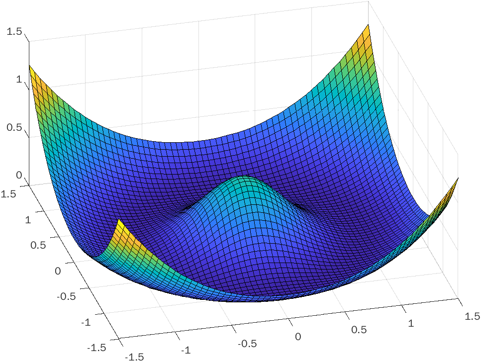
and set F:ℝ2→ℝF:{\mathbb{R}}^{2}\to{\mathbb{R}}, F⁡(x):=ψ⁡(|x|)F(x):=\psi(|x|). Note that FF is a C2C^{2}-function with critical points

𝒞:=f−1​({0})={x∈ℝ2:|x|∈{0,1}},\mathcal{C}:=f^{-1}(\{0\})=\{x\in{\mathbb{R}}^{2}:|x|\in\{0,1\}\},

where we again denote by f:=∇Ff:=\nabla F the gradient of FF. For every (x1,x2)∈ℝ2(x_{1},x_{2})\in{\mathbb{R}}^{2} we let

ort⁡(x1,x2):=(−x2,x1).\mathrm{ort}(x_{1},x_{2}):=(-x_{2},x_{1}).

and denote by φ:ℝ2→[0,1]\varphi:{\mathbb{R}}^{2}\to[0,1] a rotationally invariant C∞C^{\infty}-function with

φ|B⁡(0,2)\B⁡(0,23)≡1​ and ​φ|B⁡(0,12)∪B​(0,3)c≡0.\varphi|_{B(0,2)\backslash B(0,\frac{2}{3})}\equiv 1\text{ \ and \ }\varphi|_{B(0,\frac{1}{2})\cup B(0,3)^{c}}\equiv 0.

Consider the SDE

d​Xt=(−f⁡(Xt)+ort⁡(Xt)​||Xt|−1|)​d​t+1t+1​φ​(Xt)​d​WtdX_{t}=\Bigl(-f(X_{t})+\mathrm{ort}(X_{t})\,||X_{t}|-1|\Bigr)\,dt+\frac{1}{t+1}\varphi(X_{t})\,dW_{t}

started in a point x0∈ℝ2\{0}x_{0}\in{\mathbb{R}}^{2}\backslash\{0\}, where (Wt)t≥0(W_{t})_{t\geq 0} is a 22-dimensional Brownian motion with initial value W0=0W_{0}=0.

Theorem 4.1.
  1. (i)

    FF is a Łojasiewicz-function.

  2. (ii)

    ℙ⁡(ℂ∩𝕃)=1{\mathbb{P}}({\mathbb{C}}\cap{\mathbb{L}})=1.

  3. (iii)

    Almost surely, (Xt)t≥0(X_{t})_{t\geq 0} does not converge.

Refer to caption
Figure 1. (a) Graph of FF
Refer to caption
Figure 2. (b) Negative gradient field
Refer to caption
Figure 3. (c) Vectorfield of the drift

The proof is based on the following proposition.

Proposition 4.2.

For t≥0t\geq 0 consider the stopping time

Tt:=inf{s≥t:Xs∉B⁡(0,2)\B⁡(0,23)}.T_{t}:=\inf\bigl\{s\geq t:X_{s}\not\in B(0,2)\backslash B(0,\mbox{$\frac{2}{3}$})\bigr\}.
  1. (i)

    ℙ⁡(ℂ∩𝕃)=1{\mathbb{P}}({\mathbb{C}}\cap{\mathbb{L}})=1 and, almost surely, limt→∞|Xt|=1\lim_{t\to\infty}|X_{t}|=1. In particular, almost surely, for all sufficiently large tt, Tt=∞T_{t}=\infty.

  2. (ii)

    For every t≥0t\geq 0, (Z¯s)s≥t:=(|Xs|−1)s≥t(\bar{Z}_{s})_{s\geq t}:=(|X_{s}|-1)_{s\geq t} solves on the random time interval [t,Tt][t,T_{t}] the SDE

    d​Z¯s=(−2​Z¯s+12​1Z¯s+1​1(s+1)2)​d​s+1s+1​d​Bsd\bar{Z}_{s}=\Bigl(-2\bar{Z}_{s}+\frac{1}{2}\frac{1}{\bar{Z}_{s}+1}\frac{1}{(s+1)^{2}}\Bigr)\,ds+\frac{1}{s+1}dB_{s}

    where Bs:=∫ts1|Xu|​⟨Xu,d​Wu⟩B_{s}:=\int_{t}^{s}\frac{1}{|X_{u}|}\langle X_{u},dW_{u}\rangle is a Brownian motion.

  3. (iii)

    For t≥0t\geq 0 let (Zs(t))s≥t(Z_{s}^{(t)})_{s\geq t} denote the solution to

    (14) Zt(t)=Z¯t​ and ​d​Zs(t)=−2​Zs(t)​d​s+1s+1​d​Bs\displaystyle Z^{(t)}_{t}=\bar{Z}_{t}\text{ \ and \ }dZ^{(t)}_{s}=-2Z^{(t)}_{s}\,ds+\frac{1}{s+1}dB_{s}

    Then,

    ∫tTt|Z¯s−Zs(t)|​𝑑s≤12​1t+1.\int_{t}^{T_{t}}|\bar{Z}_{s}-Z^{(t)}_{s}|\,ds\leq\frac{1}{2}\frac{1}{t+1}.
Proof.

(i): For the choice

αt:=−f⁡(Xt)+ort⁡(Xt)||Xt|−1| and ​βt:=1t+1​φ​(Xt)​𝕀2\alpha_{t}:=-f(X_{t})+\mathrm{ort}(X_{t})\,||X_{t}|-1|\text{ \ and \ }\beta_{t}:=\frac{1}{t+1}\varphi(X_{t})\,\mathbb{I}_{2}

(Xt)t≥0(X_{t})_{t\geq 0} solves the SDE (1). We verify that the events 𝔹\mathbb{B} and ℂ{\mathbb{C}} are almost sure events. Note that the diffusivity on B⁡(0,12)∪B​(0,3)cB(0,\frac{1}{2})\cup B(0,3)^{c} is zero and that the vector field pushes (Xt)t≥0(X_{t})_{t\geq 0} towards values in B⁡(0,3)¯\B⁡(0,12)\overline{B(0,3)}\backslash B(0,\frac{1}{2}). Hence, from a deterministic time, say t0t_{0}, onwards the process (Xt)t≥0(X_{t})_{t\geq 0} stays on the compact set B⁡(0,3)¯\B⁡(0,12)\overline{B(0,3)}\backslash B(0,\frac{1}{2}). On the latter compact set FF, ∇F\nabla F and the Hessian HH of FF are uniformly bounded since FF is C2C^{2}. Therefore, 𝔹\mathbb{B} is an almost sure set.

For t≥t0t\geq t_{0}, by orthogonality of ff and ort\mathrm{ort} one has

⟨f⁡(Xt),−αt⟩=|f⁡(Xt)|2\langle f(X_{t}),-\alpha_{t}\rangle=|f(X_{t})|^{2}

and, additionally,

|αt|=|−f⁡(Xt)+ort⁡(Xt)|​|Xt​|−1||≤|f⁡(Xt)|⏟=2​|1−|Xt||+|Xt|⏟≤3​||Xt|−1|≤5|1−|Xt||=52​|f⁡(Xt)||\alpha_{t}|=|-f(X_{t})+\mathrm{ort}(X_{t})||X_{t}|-1||\leq\underbrace{|f(X_{t})|}_{=2|1-|X_{t}||}+\underbrace{|X_{t}|}_{\leq 3}\,||X_{t}|-1|\leq 5|1-|X_{t}||=\frac{5}{2}|f(X_{t})|

Moreover,

∫0∞|βs|F2​𝑑s≤∫0∞1(s+1)2|𝕀2|F2​𝑑s=2​∫0∞1(s+1)2​𝑑s<∞.\int_{0}^{\infty}|\beta_{s}|_{F}^{2}\,ds\leq\int_{0}^{\infty}\frac{1}{(s+1)^{2}}|\mathbb{I}_{2}|_{F}^{2}\,ds=2\int_{0}^{\infty}\frac{1}{(s+1)^{2}}\,ds<\infty.

Consequently, ℂ{\mathbb{C}} is an almost sure event. By Theorem 1.1, (f⁡(Xt))t≥0(f(X_{t}))_{t\geq 0} converges, almost surely, to zero so that limt→∞|Xt|=1\lim_{t\to\infty}|X_{t}|=1, almost surely.

(ii): Note that |⋅|:ℝ2∖{0}→ℝ|\cdot|:{\mathbb{R}}^{2}\setminus\{0\}\to{\mathbb{R}} is C∞C^{\infty} and, on [t,Tt][t,T_{t}], −f⁡(Xt)=−2​Z¯t​Xt|Xt|-f(X_{t})=-2\bar{Z}_{t}\frac{X_{t}}{|X_{t}|} as well as ⟨Xt,ort⁡(Xt)⟩=0\langle X_{t},\mathrm{ort}(X_{t})\rangle=0, so that with the Itô-formula we get

d​Z¯s\displaystyle d\bar{Z}_{s} =1|Xs|​⟨Xs,d​Xs⟩+12​1(s+1)2​1|Xs|​d​s\displaystyle=\frac{1}{|X_{s}|}\langle X_{s},dX_{s}\rangle+\frac{1}{2}\frac{1}{(s+1)^{2}}\frac{1}{|X_{s}|}ds
=(−2​Z¯s+12​1Z¯s+1​1(s+1)2)​d​s+1s+1​d​Bs.\displaystyle=\Bigl(-2\bar{Z}_{s}+\frac{1}{2}\frac{1}{\bar{Z}_{s}+1}\frac{1}{(s+1)^{2}}\Bigr)\,ds+\frac{1}{s+1}dB_{s}.

(iii): Fix t≥0t\geq 0 and consider (Υs(t))s≥t:=(Z¯s−Zs(t))s≥t(\Upsilon^{(t)}_{s})_{s\geq t}:=(\bar{Z}_{s}-Z^{(t)}_{s})_{s\geq t}. Then on [t,Tt][t,T_{t}]

d​Υs(t)=−2​Υs(t)​d​s+12​1Z¯s+1​1(s+1)2​d​s.d\Upsilon^{(t)}_{s}=-2\Upsilon_{s}^{(t)}\,ds+\frac{1}{2}\frac{1}{\bar{Z}_{s}+1}\frac{1}{(s+1)^{2}}\,ds.

With Υt(t)=0\Upsilon^{(t)}_{t}=0 we thus get that for t≤s≤Ttt\leq s\leq T_{t}

Υs(t)=12​∫tse−2​(s−u)​1Z¯u+1​1(u+1)2​𝑑u≤∫tse−2​(s−u)​1(u+1)2​𝑑u,\Upsilon_{s}^{(t)}=\frac{1}{2}\int_{t}^{s}e^{-2(s-u)}\frac{1}{\bar{Z}_{u}+1}\frac{1}{(u+1)^{2}}\,du\leq\int_{t}^{s}e^{-2(s-u)}\frac{1}{(u+1)^{2}}\,du,

where we used that for t≤u≤Ttt\leq u\leq T_{t}, 1Z¯u+1≤2\frac{1}{\bar{Z}_{u}+1}\leq 2. We thus get with Fubini that

∫tTt|Z¯s−Zs(t)|​𝑑s\displaystyle\int_{t}^{T_{t}}|\bar{Z}_{s}-Z_{s}^{(t)}|\,ds ≤∫t∞∫tse−2​(s−u)​1(u+1)2​𝑑u​𝑑s\displaystyle\leq\int_{t}^{\infty}\int_{t}^{s}e^{-2(s-u)}\frac{1}{(u+1)^{2}}\,du\,ds
=∫t∞∫u∞e−2​(s−u)​ds⏟=12​1(u+1)2​𝑑u=12​1t+1.\displaystyle=\int_{t}^{\infty}\underbrace{\int_{u}^{\infty}e^{-2(s-u)}\,ds}_{=\frac{1}{2}}\,\frac{1}{(u+1)^{2}}\,du=\frac{1}{2}\frac{1}{t+1}.

∎

Now, let t≥0t\geq 0 and x0∈ℝx_{0}\in{\mathbb{R}} and let (Zs)s≥t(Z_{s})_{s\geq t} be the solution of the SDE

(15) d​Zs=−2​Zs​d​s+(s+1)−1​d​Bs, with ​Zt=x0.\displaystyle dZ_{s}=-2Z_{s}\,ds+(s+1)^{-1}\,dB_{s},\text{ with }Z_{t}=x_{0}.

Using Itô’s lemma and the Dubins-Schwarz theorem it is straight-forward to see that one can represent the solution as

(Zs)s≥t=(e−2​s​B~gs)s≥t,(Z_{s})_{s\geq t}=(e^{-2s}\tilde{B}_{g_{s}})_{s\geq t},

where (B~s)s≥gt(\tilde{B}_{s})_{s\geq g_{t}} is a Brownian motion started at time gtg_{t} in B~gt=e2​t​x0\tilde{B}_{g_{t}}=e^{2t}x_{0} and (gs)s≥0(g_{s})_{s\geq 0} is given by

gs:=∫0s(u+1)−2​e4​u​𝑑u∼14​(s+1)−2​e4​s.g_{s}:=\int_{0}^{s}(u+1)^{-2}e^{4u}\,du\sim\frac{1}{4}(s+1)^{-2}e^{4s}.

Note that gs≤e4​s(s+1)2g_{s}\leq\frac{e^{4s}}{(s+1)^{2}}.

Lemma 4.3.

For every t≥0t\geq 0 and x0∈ℝx_{0}\in{\mathbb{R}} the solution (Zs)s≥t(Z_{s})_{s\geq t} of (15) satisfies

∫t∞|Zs|​𝑑s=∞,almost surely.\int_{t}^{\infty}|Z_{s}|\,ds=\infty,\qquad\text{almost surely.}
Proof.

We let for s≥ts\geq t, B¯s:=B~gs−e2​t​x0\bar{B}_{s}:=\tilde{B}_{g_{s}}-e^{2t}x_{0} and note that

|∫tu|Zs|​𝑑s−∫tu|e−2​s​B¯s|​𝑑s|≤|x0|​∫0∞e−2​s​𝑑s=12​|x0|.\Bigl|\int_{t}^{u}|Z_{s}|\,ds-\int_{t}^{u}|e^{-2s}\bar{B}_{s}|\,ds\Bigr|\leq|x_{0}|\int_{0}^{\infty}e^{-2s}\,ds=\mbox{$\frac{1}{2}$}|x_{0}|.

Hence, it suffices to show that ∫t∞|e−2​s​B¯s|​𝑑s=∞\int_{t}^{\infty}|e^{-2s}\bar{B}_{s}|\,ds=\infty, almost surely. Set

κ:=∫ℝ12​π|x|e−x2/2dx=2π.\kappa:=\int_{\mathbb{R}}\frac{1}{\sqrt{2\pi}}|x|\,e^{-x^{2}/2}\,dx=\sqrt{\frac{2}{\pi}}.

One has

𝔼⁡[∫tue−2​s​|B¯s|​𝑑s]\displaystyle{\mathbb{E}}\Bigl[\int_{t}^{u}e^{-2s}|\bar{B}_{s}|\,ds\Bigr] =∫tue−2​s​𝔼​[|B¯s|]​𝑑s=κ​∫tue−2​s​gs−gt​𝑑s.\displaystyle=\int_{t}^{u}e^{-2s}{\mathbb{E}}[|\bar{B}_{s}|]\ ds=\kappa\int_{t}^{u}e^{-2s}\sqrt{g_{s}-g_{t}}\,ds.

Using that gs∼14​(s+1)−2​e4​sg_{s}\sim\frac{1}{4}(s+1)^{-2}e^{4s} we get that

κ​∫tue−2​s​gs−gt​𝑑s∼12​κ​∫tu(s+1)−1​𝑑s∼12​κ​log⁡u.\kappa\int_{t}^{u}e^{-2s}\sqrt{g_{s}-g_{t}}\,ds\sim\mbox{$\frac{1}{2}$}\kappa\int_{t}^{u}(s+1)^{-1}\,ds\sim\mbox{$\frac{1}{2}$}\kappa\log u.

To estimate the variance we first show that for v≥u≥tv\geq u\geq t we have

(16) cov⁡(|B¯u|,|B¯v|)≤gv−gt.\displaystyle\mathrm{cov}(|\bar{B}_{u}|,|\bar{B}_{v}|)\leq g_{v}-g_{t}.

Indeed,

𝔼⁡[|B¯v​B¯u|]\displaystyle{\mathbb{E}}[|\bar{B}_{v}\bar{B}_{u}|] ≤𝔼⁡[B¯u2]+𝔼⁡[|B¯v−B¯u|]​𝔼​[|B¯u|]\displaystyle\leq{\mathbb{E}}[\bar{B}_{u}^{2}]+{\mathbb{E}}[|\bar{B}_{v}-\bar{B}_{u}|]\,{\mathbb{E}}[|\bar{B}_{u}|]
≤gu−gt+κ2​gv−gu​gu−gt\displaystyle\leq g_{u}-g_{t}+\kappa^{2}\sqrt{g_{v}-g_{u}}\sqrt{g_{u}-g_{t}}

and

𝔼⁡[|B¯v|]​𝔼​[|B¯u|]=κ2​gv−gt​gu−gt.{\mathbb{E}}[|\bar{B}_{v}|]\,{\mathbb{E}}[|\bar{B}_{u}|]=\kappa^{2}\sqrt{g_{v}-g_{t}}\sqrt{g_{u}-g_{t}}.

Thus (16) follows since gu≥gtg_{u}\geq g_{t}. We conclude that for all ℓ≥t\ell\geq t

Var⁡(∫tℓe−2​s​|B¯s|​𝑑s)\displaystyle\mathrm{Var}\Bigl(\int_{t}^{\ell}e^{-2s}|\bar{B}_{s}|\,ds\Bigr) =∫tℓ∫tℓe−2​(u+v)​cov​(|B¯u|,|B¯v|)​𝑑u​𝑑v\displaystyle=\int_{t}^{\ell}\int_{t}^{\ell}e^{-2(u+v)}\mathrm{cov}(|\bar{B}_{u}|,|\bar{B}_{v}|)\ du\,dv
≤2​∫tℓ∫uℓe−2​(u+v)​gu​𝑑v​𝑑u\displaystyle\leq 2\int_{t}^{\ell}\int_{u}^{\ell}e^{-2(u+v)}g_{u}\ dv\,du
≤∫0ℓe−4​u​gu​𝑑u≤∫0ℓ1(u+1)2​𝑑u≤1.\displaystyle\leq\int_{0}^{\ell}e^{-4u}g_{u}\,du\leq\int_{0}^{\ell}\frac{1}{(u+1)^{2}}\,du\leq 1.

Hence, as a consequence of the Chebyshev inequality one gets that

∫t∞e−2​s|B¯s|𝑑s=limu→∞∫tue−2​s​|B¯s|​𝑑s=∞,almost surely.\int_{t}^{\infty}e^{-2s}|\bar{B}_{s}|\,ds=\lim_{u\to\infty}\int_{t}^{u}e^{-2s}|\bar{B}_{s}|\,ds=\infty,\quad\text{almost surely.}

∎

Proof of Theorem 4.1.

(i): We first verify that FF is a Łojasiewicz-function. We need to analyse the critical points only. One has

Hess​F​(0)=(−600−6)\text{Hess}\,F(0)=\begin{pmatrix}-6&0\\ 0&-6\end{pmatrix}

so that the Hessian has full rank at 00 which implies validity of a Łojasiewicz-inequality with θ=12\theta=\frac{1}{2} on an appropriate neighbourhood of 00. Next, let x∈ℝ2x\in{\mathbb{R}}^{2} with |x|=1|x|=1. Since ψ′′​(1)=2\psi^{\prime\prime}(1)=2, ψ\psi satisfies a Łojasiewicz-inequality

|ψ′​(r)|≥Ł​|ψ⁡(r)−ψ⁡(1)|12|\psi^{\prime}(r)|\geq\L|\psi(r)-\psi(1)|^{\frac{1}{2}}

for all r∈[1−ε,1+ε)r\in[1-\varepsilon,1+\varepsilon) and appropriately fixed ε∈(0,12]\varepsilon\in(0,\frac{1}{2}] and Ł>0\L>0. Consequently, for y∈B⁡(0,1+ε)\B⁡(0,1−ε)y\in B(0,1+\varepsilon)\backslash B(0,1-\varepsilon) one has

|f⁡(y)|=|ψ′​(|y|)|≥Ł​|ψ⁡(|y|)−ψ⁡(1)|1/2=Ł​|F⁡(y)−F⁡(x)|1/2.|f(y)|=|\psi^{\prime}(|y|)|\geq\L\,|\psi(|y|)-\psi(1)|^{1/2}=\L\,|F(y)-F(x)|^{1/2}.

(ii): has been shown in Prop. 4.2.

(iii): We conceive (Xt)t≥0(X_{t})_{t\geq 0} as complex-valued process by letting

Yt:=Xt(1)+i​Xt(2)Y_{t}:=X^{(1)}_{t}+iX^{(2)}_{t}

and note that (since (Yt)t≥0(Y_{t})_{t\geq 0} does not hit 00) there is a continuous adapted process (Φs)s≥0(\Phi_{s})_{s\geq 0} satisfying

Ys=|Xs|​ei​Φs.Y_{s}=|X_{s}|e^{i\Phi_{s}}.

Now on [t,Tt][t,T_{t}]

d​Φs=||Xs|−1|​d​s+1|Xs|2​1s+1​⟨ort⁡(Xs),d​Ws⟩\displaystyle d\Phi_{s}=||X_{s}|-1|\,ds+\frac{1}{|X_{s}|^{2}}\frac{1}{s+1}\langle\mathrm{ort}(X_{s}),dW_{s}\rangle

so that

d​⟨Ψ⟩s=1|Xs|2​1(s+1)2​d​s.d\langle\Psi\rangle_{s}=\frac{1}{|X_{s}|^{2}}\frac{1}{(s+1)^{2}}\,ds.

We thus get that

∫tTtd​⟨Ψ⟩s=∫tTt1|Xs|2​1(s+1)2​𝑑s≤94​∫t∞1(s+1)2​𝑑s<∞\int_{t}^{T_{t}}d\langle\Psi\rangle_{s}=\int_{t}^{T_{t}}\frac{1}{|X_{s}|^{2}}\frac{1}{(s+1)^{2}}\,ds\leq\mbox{$\frac{9}{4}$}\int_{t}^{\infty}\frac{1}{(s+1)^{2}}\,ds<\infty

so that ∫tTt∧s1|Xu|2​1u+1​⟨ort⁡(Xu),d​Wu⟩\int_{t}^{T_{t}\wedge s}\frac{1}{|X_{u}|^{2}}\frac{1}{u+1}\langle\mathrm{ort}(X_{u}),dW_{u}\rangle converges almost surely as s→∞s\to\infty, say to Ψ¯(t)\bar{\Psi}^{(t)}. Consequently, on {Tt=∞}\{T_{t}=\infty\} one has as s→∞s\to\infty

Φs=∫ts||Xu|−1|​𝑑u+Φ¯(t)+o⁡(1),\Phi_{s}=\int_{t}^{s}||X_{u}|-1|\,du+\bar{\Phi}^{(t)}+o(1),

where o⁡(1)o(1) stands for a term converging to zero as s→∞s\to\infty. By Proposition 4.2 (iii) and Lemma 4.3, ∫ts||Xu|−1|𝑑u→∞\int_{t}^{s}||X_{u}|-1|\,du\to\infty as s→∞s\to\infty which shows that (Xt)t≥0(X_{t})_{t\geq 0} does not converge on {Tt=∞}\{T_{t}=\infty\}. The result follows by noticing that ⋃t∈ℕ{Tt=∞}\bigcup_{t\in{\mathbb{N}}}\{T_{t}=\infty\} is an almost sure set by Proposition 4.2 (i). ∎

Appendix A Criterion for staying local

Assume that FF satisfies lim|x|→∞F⁡(x)=∞\lim_{|x|\to\infty}F(x)=\infty and consider the set

𝕃1:={supt≥0∫0t(⟨f(Xs),αs⟩+12tr(βs†H(Xs)βs))ds<∞}.{\mathbb{L}}_{1}:=\Bigl\{\sup\limits_{t\geq 0}\int_{0}^{t}\bigl(\langle f(X_{s}),\alpha_{s}\rangle+\frac{1}{2}\mathrm{tr}(\beta_{s}^{\dagger}H(X_{s})\beta_{s})\bigr)\,ds<\infty\Bigr\}.

We will show that lim supt→∞|Xt|<∞\limsup_{t\to\infty}|X_{t}|<\infty, almost surely, on 𝕃1{\mathbb{L}}_{1}. By Itô’s formula

d​F​(Xt)=⟨f⁡(Xt),αt⟩​d​t+⟨f⁡(Xt),βt​d​Wt⟩+12​tr​(βt†​H​(Xt)​βt)​d​t.dF(X_{t})=\langle f(X_{t}),\alpha_{t}\rangle\,dt+\langle f(X_{t}),\beta_{t}\,dW_{t}\rangle+\frac{1}{2}\mathrm{tr}(\beta_{t}^{\dagger}H(X_{t})\beta_{t})\,dt.

Now, let n∈ℕn\in{\mathbb{N}} and consider the stopping time

Tn:=inf{t≥0:∫0t(⟨f⁡(Xs),αs⟩+12​tr​(βs†​H​(Xs)​βs))​𝑑s≥n}.T_{n}:=\inf\Bigl\{t\geq 0:\int_{0}^{t}\bigl(\langle f(X_{s}),\alpha_{s}\rangle+\frac{1}{2}\mathrm{tr}(\beta_{s}^{\dagger}H(X_{s})\beta_{s})\bigr)\,ds\geq n\Bigr\}.

and (Yt)t≥0(Y_{t})_{t\geq 0} given by

Yt:=F⁡(Xt)−∫0t(⟨f⁡(Xs),αs⟩+12​tr​(βs†​H​(Xs)​βs))​𝑑s.Y_{t}:=F(X_{t})-\int_{0}^{t}\bigl(\langle f(X_{s}),\alpha_{s}\rangle+\frac{1}{2}\mathrm{tr}(\beta_{s}^{\dagger}H(X_{s})\beta_{s})\bigr)\,ds.

Then, (YtTn)t≥0(Y_{t}^{T_{n}})_{t\geq 0} is a local martingale that is bounded from below and, thus, a supermartingale. With the martingale convergence theorem we get almost sure convergence of (YtTn)t≥0(Y_{t}^{T_{n}})_{t\geq 0} and, thus, on {Tn=∞}\{T_{n}=\infty\} we have that supt≥0F⁡(Xt)\sup_{t\geq 0}F(X_{t}) is finite, almost surely. Finally, note that

𝕃1=⋃n∈ℕ{Tn=∞},{\mathbb{L}}_{1}=\bigcup\limits_{n\in{\mathbb{N}}}\{T_{n}=\infty\},

so that lim supt→∞|Xt|<∞\limsup_{t\to\infty}|X_{t}|<\infty, almost surely, on 𝕃1{\mathbb{L}}_{1}. Note that for the choice (αt)t≥0=(−f⁡(Xt))t≥0(\alpha_{t})_{t\geq 0}=(-f(X_{t}))_{t\geq 0} we have

{supt≥0|H(Xt)|<∞ and ∫0∞|βs|F2ds<∞}⊂𝕃1\Bigl\{\sup\limits_{t\geq 0}|H(X_{t})|<\infty\text{ and }\int_{0}^{\infty}|\beta_{s}|_{F}^{2}\,ds<\infty\Bigr\}\subset{\mathbb{L}}_{1}

as well as for a compact set K⊂ℝdK\subset{\mathbb{R}}^{d}

{\displaystyle\Bigl\{ 1l{Xt∉K}(−|f(Xt)|2+12tr((βt)†H(Xt)βt))≤0 for all large t\displaystyle 1\hskip-2.78857pt\mathrm{l}_{\{X_{t}\notin K\}}(-|f(X_{t})|^{2}+\frac{1}{2}\mathrm{tr}((\beta_{t})^{\dagger}H(X_{t})\beta_{t}))\leq 0\text{ for all large }t
and ∫0∞1l{Xs∈K}|βs|F2ds<∞}⊂𝕃1.\displaystyle\text{ and }\int_{0}^{\infty}1\hskip-2.78857pt\mathrm{l}_{\{X_{s}\in K\}}|\beta_{s}|_{F}^{2}\,ds<\infty\Bigr\}\subset{\mathbb{L}}_{1}.

Acknowledgement. The authors would like to thank the two anonymous referees for their valuable comments. Funded by the Deutsche Forschungsgemeinschaft (DFG, German Research Foundation) under Germany’s Excellence Strategy EXC 2044–390685587, Mathematics Münster: Dynamics–Geometry–Structure.

References

  • [AMA05] P.-A. Absil, R. Mahony, and B. Andrews. Convergence of the iterates of descent methods for analytic cost functions. SIAM J. Optim., 16(2):531–547, 2005.
  • [Ben99] M. Benaïm. Dynamics of stochastic approximation algorithms. In Seminaire de probabilites XXXIII, pages 1–68. Springer, 1999.
  • [CHS87] T.-S. Chiang, C.-R. Hwang, and S. J. Sheu. Diffusion for global optimization in ℝn\mathbb{R}^{n}. SIAM Journal on Control and Optimization, 25(3):737–753, 1987.
  • [CMI14] T. Colding and W. Minicozzi II. Lojasiewicz inequalities and applications. In Surveys in Differential Geometry, XIX, pages 63–82. 2014.
  • [Cur44] H. B. Curry. The method of steepest descent for non-linear minimization problems. Quarterly of Applied Mathematics, 2(3):258–261, 1944.
  • [DK21] S. Dereich and S. Kassing. Convergence of stochastic gradient descent schemes for Łojasiewicz-landscapes. arXiv:2102.09385, 2021.
  • [FT21] N. Fournier and C. Tardif. On the simulated annealing in ℝd\mathbb{R}^{d}. J. Funct. Anal., 281(5):Paper No. 109086, 30, 2021.
  • [FW12] M. I. Freidlin and A. D. Wentzell. Random Perturbations of Dynamical Systems. Grundlehren der mathematischen Wissenschaften. Springer New York, 2012.
  • [Gar85] C. W. Gardiner. Handbook of stochastic methods, volume 3. springer Berlin, 1985.
  • [GH86] S. Geman and C.-R. Hwang. Diffusions for global optimization. SIAM Journal on Control and Optimization, 24(5):1031–1043, 1986.
  • [Gil00] D. T. Gillespie. The chemical Langevin equation. The Journal of Chemical Physics, 113(1):297–306, 2000.
  • [Har12] A. Haraux. Some applications of the Łojasiewicz gradient inequality. Communications on Pure & Applied Analysis, 11(6):2417, 2012.
  • [HKS89] R. A. Holley, S. Kusuoka, and D. W Stroock. Asymptotics of the spectral gap with applications to the theory of simulated annealing. Journal of functional analysis, 83(2):333–347, 1989.
  • [JKO98] R. Jordan, D. Kinderlehrer, and F. Otto. The variational formulation of the fokker–planck equation. SIAM journal on mathematical analysis, 29(1):1–17, 1998.
  • [Łoj63] S. Łojasiewicz. Une propriété topologique des sous-ensembles analytiques réels. Les équations aux dérivées partielles, 117:87–89, 1963.
  • [Łoj65] S. Łojasiewicz. Ensembles semi-analytiques. Lectures Notes IHES (Bures-sur-Yvette), 1965.
  • [Łoj84] S. Łojasiewicz. Sur les trajectoires du gradient d’une fonction analytique. (Trajectories of the gradient of an analytic function). Semin. Geom., Univ. Studi Bologna, 1982/1983:115–117, 1984.
  • [LTE17] Q. Li, C. Tai, and W. E. Stochastic modified equations and adaptive stochastic gradient algorithms. In Proceedings of the 34th International Conference on Machine Learning, volume 70, pages 2101–2110. PMLR, 06–11 Aug 2017.
  • [PdM82] J. Palis, Jr. and W. de Melo. Geometric theory of dynamical systems: an introduction. Springer Science & Business Media, 1982.
  • [SSG14] D. Schnoerr, G. Sanguinetti, and R. Grima. The complex chemical Langevin equation. The Journal of Chemical Physics, 141(2):07B606_1, 2014.
  • [vK92] N. G. van Kampen. Stochastic processes in physics and chemistry, volume 1. Elsevier, 1992.