Analysis of error localization of Chebyshev spectral approximations

Haiyong Wang¹¹ 1 School of Mathematics and Statistics, Huazhong University of Science and Technology, Wuhan 430074, P. R. China. E-mail: haiyongwang@hust.edu.cn ²² 2 Hubei Key Laboratory of Engineering Modeling and Scientific Computing, Huazhong University of Science and Technology, Wuhan 430074, P. R. China.

Abstract

Chebyshev spectral methods are widely used in numerical computations. When the underlying function has a singularity, it has been observed by L. N. Trefethen in 2011 that its Chebyshev interpolants exhibit an error localization property, that is, their errors in a neighborhood of the singularity are obviously larger than elsewhere. In this paper, we first present a pointwise error analysis for Chebyshev projections of functions with a singularity and prove that the rate of convergence of Chebyshev projections of degree $n$ at each point away from the singularity is one power of $n$ faster than that of at the singularity. This gives a rigorous justification for the error localization of Chebyshev projections. We then extend the framework of our analysis to Chebyshev interpolants, Chebyshev spectral differentiations and Legendre projections and justify their error localization using similar arguments. As a result, we find that Chebyshev spectral differentiations converge faster than their best counterparts except in a neighborhood of the singularity and, in the particular case where the singularity is located in the interior of interval, they converge even faster than their best counterparts in the maximum norm.

Keywords: Chebyshev projections, pointwise error estimates, error localization, best approximations, Chebyshev interpolants, spectral differentiation, Legendre projections

AMS subject classifications: 41A10, 41A25, 41A50

1 Introduction

Spectral approximations, such as Chebyshev and Legendre projections and interpolants, are invaluable and powerful methods and they play an important role in numerous practical applications, including Gauss and Clenshaw-Curtis quadrature, rootfinding and spectral methods for differential and integral equations (see, e.g., [7, 8, 10, 19, 22, 24, 26, 27, 29]). Of particular importance are Chebyshev spectral approximations, which have several remarkable advantages including: (i) they are near-best approximations, that is, their approximation quality in the maximum norm is close to that of best approximations [17, 19, 22, 29, 34]; (ii) the discrete Chebyshev transforms, i.e., the transforms between the values at the Chebyshev points and the Chebyshev expansion coefficients, can be achieved rapidly by means of the fast Fourier transform (FFT) [19, 24]; (iii) the evaluation of Chebyshev interpolants can be achieved stably and rapidly using the barycentric formula [4, 14]. Due to these attractive advantages, Chebyshev spectral approximations are widely used in many branches of numerical analysis. We refer the interested reader to [11, 19, 22, 29] for more extensive overview.

Let $\mathrm{\Omega}:=[-1,1]$ and let $T_{k}(x)$ be the Chebyshev polynomial of the first kind of degree $k$ , i.e., $T_{k}(x)=\cos(k\arccos(x))$ . It is well known that the Chebyshev polynomials $\{T_{k}(x)\}$ are orthogonal with respect to the weight function $(1-x^{2})^{-1/2}$ on $\mathrm{\Omega}$ . If $f$ satisfies the Dini-Lipschitz continuous on $\mathrm{\Omega}$ , then it has the following uniformly convergent Chebyshev series [19, Theorem 5.7]

\displaystyle f(x)=\sum_{k=0}^{\infty}{{}^{\prime}}a_{k}T_{k}(x),\quad a_{k}=\frac{2}{\pi}\int_{\Omega}\frac{f(x)T_{k}(x)}{\sqrt{1-x^{2}}}\mathrm{d}x,

(1.1)

where the prime indicates that the first term of the sum should be halved. Truncating the above infinite series after the first $n+1$ terms, we obtain the Chebyshev projection of degree $n$ of $f$ , i.e.,

\displaystyle f_{n}(x)=\sum_{k=0}^{n}{{}^{\prime}}a_{k}T_{k}(x).

(1.2)

Let $\Pi_{n}$ denote the space of polynomials of degree at most $n$ and let $p_{n}^{*}$ denote the best approximation in $\Pi_{n}$ to $f$ in the maximum norm, i.e., $\|f-p_{n}^{*}\|_{L^{\infty}(\Omega)}=\min_{h\in\Pi_{n}}\|f-h\|_{L^{\infty}(\Omega)}$ . It is well known that $p_{n}^{*}$ exists and is unique whenever $f\in\mathrm{C}(\mathrm{\Omega})$ . We are interested in the comparison of $f_{n}$ and $p_{n}^{*}$ . From the viewpoint of minimizing the maximum error of approximants, it is evident that $p_{n}^{*}$ is better than $f_{n}$ . From the viewpoint of practical convenience, however, it is evident that $f_{n}$ is preferable to $p_{n}^{*}$ since $f_{n}$ depends linearly on $f$ and its implementations can be achieved efficiently by means of the FFT. In contrast, $p_{n}^{*}$ depends nonlinearly on $f$ and its implementation must resort to iterative methods, which results in an expensive computational cost, especially when $n$ is large. We further consider the difference in approximation quality between $p_{n}^{*}$ and $f_{n}$ . A classical result associated with this issue are the following inequalities [22, Theorem 3.3]

\displaystyle\|f-p_{n}^{*}\|_{L^{\infty}(\Omega)}\leq\|f-f_{n}\|_{L^{\infty}(\Omega)}<\left(4+\frac{4}{\pi^{2}}\log n\right)\|f-p_{n}^{*}\|_{L^{\infty}(\Omega)},

(1.3)

from which we see that the maximum error of $f_{n}$ is worse than that of $p_{n}^{*}$ by at most a logarithmic factor. Direct calculation shows that $\|f-f_{n}\|_{L^{\infty}(\Omega)}<9.6\|f-p_{n}^{*}\|_{L^{\infty}(\Omega)}$ for $n\leq 10^{6}$ , which means that the maximum error of $p_{n}^{*}$ will never be better than that of $f_{n}$ by one digit even if the degree of both methods is one million. Regarding (1.3), we further ask the following question: Is $p_{n}^{*}$ really better than $f_{n}$ by a logarithmic factor? At first glance, this question has already been answered by the inequalities above. However, they only answer this question from the viewpoint of measuring the maximum error of both approximants. If we compare both approximants from the viewpoint of the rate of pointwise convergence, the inequalities above might be one-sided or even misleading. To illustrate this, we plot the error curves of $f_{n}$ and $p_{n}^{*}$ for the test function $f(x)=|x-1/2|^{\alpha}$ and we test two different values of $\alpha$ and $n$ , respectively. Throughout the paper, $p_{n}^{*}$ is calculated by the barycentric-Remez algorithm in Chebfun (see [11]). The pointwise error curves are depicted in Figure 1, which suggest that:

Refer to caption — Figure 1: Pointwise error curves of $f_{n}$ and $p_{n}^{*}$ for $n=10$ (left) and $n=100$ (right). The top row corresponds to $\alpha=1$ and the bottom row corresponds to $\alpha=3/2$ .

(i)

The error of $p_{n}^{*}$ equioscillates over the whole interval. The error of $f_{n}$ , however, is highly localized for large $n$ , that is, the maximum errors of $f_{n}$ are always attained at a small neighborhood of the singularity and the larger $n$ , the narrower the neighborhood that the pointwise error curves attain their maximum;
(ii)

Comparing the accuracy of $f_{n}$ and $p_{n}^{*}$ , we observe that the accuracy of $p_{n}^{*}$ is better than that of $f_{n}$ only in a small neighborhood of the singularity. Otherwise, the accuracy of $p_{n}^{*}$ is worse than that of $f_{n}$ .

We are not the first to notice these observations. In fact, Trefethen in [28] observed a similar phenomenon from the pointwise error curve of Chebyshev interpolant. He further made the following comments:

“Which approximation would be more useful in an application? I think the only reasonable answer is, it depends. Sometimes one really does need a guarantee about worst-case behavior. In other situations, it would be wasteful to sacrifice so much accuracy over 95% of the range just to gain one bit of accuracy in a small subinterval.”

However, no theoretical justification was given to explain these observations.

In this work, we aim to justify the error localization property of Chebyshev spectral approximations and present a detailed analysis of their pointwise rate of convergence for functions with singularities. For ease of presentation, we restrict our analysis to the following model function

\displaystyle f(x)=|x-\xi|^{\alpha}g(x),

(1.4)

where $\xi\in\Omega$ and $\alpha>0$ is not an even integer whenever $\xi\in(-1,1)$ and is not an integer whenever $\xi=\pm 1$ , and $g\in{C}^{\infty}(\Omega)$ and $g(\xi)\neq 0$ . In order to compare the pointwise rates of convergence of $f_{n}$ and $p_{n}^{*}$ , we define the set

\displaystyle V_{0}(x)=\left\{x\in\Omega:~\lim_{n\rightarrow\infty}\frac{|f(x)-f_{n}(x)|}{\|f-p_{n}^{*}\|_{L^{\infty}(\Omega)}}=0\right\}.

(1.5)

Note that we have used $\|f-p_{n}^{*}\|_{L^{\infty}(\Omega)}$ instead of $|f(x)-p_{n}^{*}(x)|$ in the denominator due to the equioscillation property of the error of $p_{n}^{*}$ . It is easily seen that the set $V_{0}(x)$ contains all the points on $\Omega$ at which $f_{n}$ converges faster than $p_{n}^{*}$ . Our main result states that the rate of convergence of $f_{n}$ is one power of $n$ faster than that of $p_{n}^{*}$ whenever $x$ is away from $\xi$ and both $f_{n}$ and $p_{n}^{*}$ converge at the same rate whenever $x=\xi$ . Therefore, we can deduce that $V_{0}(x)=\Omega\backslash\{\xi\}$ and this gives a rigorous justification of those observations displayed in Figure 1. We show that the key ingredient for explaining the error localization of $f_{n}$ is to understand the asymptotic behavior of the following two functions

\displaystyle\Psi_{\nu}^{\mathrm{C}}(\theta,n)=\sum_{k=n+1}^{\infty}\frac{\cos(k\theta)}{k^{\nu+1}},\qquad\Psi_{\nu}^{\mathrm{S}}(\theta,n)=\sum_{k=n+1}^{\infty}\frac{\sin(k\theta)}{k^{\nu+1}},

(1.6)

where $\theta\in\mathbb{R}$ , $n\in\mathbb{N}_{0}:=\mathbb{N}\cup\{0\}$ and $\nu>-1$ whenever $\theta(\mathrm{mod}~2\pi)\neq 0$ and $\nu>0$ whenever $\theta(\mathrm{mod}~2\pi)=0$ . As will be shown later, these two functions are intimately related to the Lerch’s transcendent function and its special case Hurwitz zeta function (see, e.g., [20, Chapter 25]) and their asymptotic behavior has a crucial distinction between $\theta(\mathrm{mod}~2\pi)\neq 0$ and $\theta(\mathrm{mod}~2\pi)=0$ . With this key finding in hand, we are able to clearly explain not only the error localization of Chebyshev projections, but also the same property of Chebyshev interpolants, Chebyshev spectral differentiations and Legendre projections. As a result, we show that Chebyshev spectral differentiations converge faster than their best counterparts except in a neighborhood of $\xi$ and, in the particular case where $\xi\in(-1,1)$ , they converge even faster than their best counterparts in the maximum norm. Our results provide further justification for the use of Chebyshev spectral methods in numerical computations.

The paper is organized as follows. In section 2, we present a thorough analysis of the pointwise error estimates of Chebyshev projections. In section 3, we extend our analysis to a more general setting, including superconvergent points of Chebyshev projections, Chebyshev interpolants, Chebyshev spectral differentiation and Legendre projections. In section 4, we finish this paper with some concluding remarks.

2 Pointwise error estimates of Chebyshev projections

In this section, we present pointwise error estimates of Chebyshev projections for the model function defined in (1.4). Our main result will provide a thorough understanding of the pointwise error behavior of Chebyshev projections for functions with a singularity. For notational simplicity, we introduce

\displaystyle\varphi_{\xi}^{\pm}(x)=\frac{\arccos(x)\pm\arccos(\xi)}{2},

(2.1)

and we will drop the argument $x$ in $\varphi_{\xi}^{\pm}(x)$ whenever there is no ambiguity.

Before stating our main result, we provide two useful lemmas that will be used in the proof of our main result.

Lemma 2.1.

Let $f$ be the function defined in (1.4) and let $a_{k}$ be its $k$ th Chebyshev coefficient.

(i)

If $\xi\in(-1,1)$ , then for $k\gg 1$ , we have

\displaystyle a_{k}=\mathcal{I}_{1}(\alpha,\xi)\frac{T_{k}(\xi)}{k^{\alpha+1}}+\mathcal{I}_{2}(\alpha,\xi)\frac{U_{k-1}(\xi)}{k^{\alpha+2}}+O(k^{-\alpha-3}),

(2.2)

where $U_{k}(x)$ is the Chebyshev polynomial of the second kind of degree $k$ and

	$\displaystyle\mathcal{I}_{1}(\alpha,\xi)$	$\displaystyle=-\frac{4(1-\xi^{2})^{\alpha/2}\Gamma(\alpha+1)}{\pi}\sin\left(\frac{\alpha\pi}{2}\right)g(\xi),$
	$\displaystyle\mathcal{I}_{2}(\alpha,\xi)$	$\displaystyle=-\frac{4(1-\xi^{2})^{\alpha/2}\Gamma(\alpha+2)}{\pi}\sin\left(\frac{\alpha\pi}{2}\right)\left[(1-\xi^{2})g{{}^{\prime}}(\xi)-\frac{\alpha\xi}{2}g(\xi)\right].$

(ii)

If $\xi=\pm 1$ , then for $k\gg 1$ , we have

\displaystyle a_{k}=\mathcal{B}(\alpha,\xi)\frac{T_{k}(\xi)}{k^{2\alpha+1}}+O(k^{-2\alpha-3}),\quad\mathcal{B}(\alpha,\xi)=-\frac{\sin(\alpha\pi)\Gamma(2\alpha+1)}{2^{\alpha-1}\pi}g(\xi).

(2.3)

Proof.

As for (i), it follows from Theorem 2.1 in [16]. As for (ii), it follows from Theorem 2.2 in [33]. ∎

Lemma 2.2.

Let $\Psi_{\nu}^{\mathrm{C}}(\theta,n)$ and $\Psi_{\nu}^{\mathrm{S}}(\theta,n)$ be the functions defined in (1.6). For $n\gg 1$ , the following two statements hold:

(i)

If $\theta(\mathrm{mod}~2\pi)\neq 0$ and $\nu>-1$ , we have

\displaystyle\Psi_{\nu}^{\mathrm{C}}(\theta,n)

\displaystyle=-\frac{\sin((2n+1)\theta/2)}{2\sin(\theta/2)}n^{-\nu-1}+O(n^{-\nu-2}),

(2.4)

and

\displaystyle\Psi_{\nu}^{\mathrm{S}}(\theta,n)

\displaystyle=\frac{\cos((2n+1)\theta/2)}{2\sin(\theta/2)}n^{-\nu-1}+O(n^{-\nu-2}).

(2.5)

(ii)

If $\theta(\mathrm{mod}~2\pi)=0$ and $\nu>0$ , we have

$\displaystyle\Psi_{\nu}^{\mathrm{C}}(\theta,n)$ $\displaystyle=\frac{1}{\nu}n^{-\nu}-\frac{1}{2}n^{-\nu-1}+O(n^{-\nu-2}).$ (2.6)

Proof.

We notice that

\displaystyle\Psi_{\nu}^{\mathrm{C}}(\theta,n)+i\Psi_{\nu}^{\mathrm{S}}(\theta,n)

\displaystyle=e^{i(n+1)\theta}\Phi(e^{i\theta},\nu+1,n+1),

where $i$ is the imaginary unit and $\Phi(z,s,a)$ is the Lerch’s transcendent function defined by (see, e.g., [20, §25.14(i)] and [12])

\displaystyle\Phi(z,s,a)=\sum_{k=0}^{\infty}\frac{z^{k}}{(k+a)^{s}},

(2.7)

and where $a\neq 0,-1,\ldots$ , $s\in\mathbb{C}$ whenever $|z|<1$ and $\Re(s)>1$ whenever $|z|=1$ . For other values of $z$ , $\Phi(z,s,a)$ is defined by analytic continuation. Moreover, the Lerch’s transcendent function reduces to the Hurwitz zeta functions whenever $z=1$ , i.e.,

\displaystyle\Phi(1,s,a)=\sum_{k=0}^{\infty}\frac{1}{(k+a)^{s}}:=\zeta(s,a),

(2.8)

where $\zeta(s,a)$ is the Hurwitz zeta functions [20, §25.11(i)]. As for (i), we recall from [12, Theorem 1] that $\Phi(z,s,a)=(1-z)^{-1}a^{-s}+O(a^{-s-1})$ for $z\in\mathbb{C}\setminus[1,\infty)$ , $s\in\mathbb{C}$ and $|a|\rightarrow\infty$ , and thus

\displaystyle\Psi_{\nu}^{\mathrm{C}}(\theta,n)+i\Psi_{\nu}^{\mathrm{S}}(\theta,n)=\frac{e^{i(n+1)\theta}}{1-e^{i\theta}}n^{-\nu-1}+O(n^{-\nu-2}).

The results (2.4) and (2.5) follow from the above equation by taking real and imaginary parts, respectively. As for (ii), from [20, Equation (25.11.3)] we know that $\Psi_{\nu}^{\mathrm{C}}(\theta,n)=\zeta(\nu+1,n+1)=\zeta(\nu+1,n)-n^{-\nu-1}$ . The result (2.6) then follows from the asymptotic expansion of $\zeta(\nu,n)$ in [20, Equation (25.11.43)]. This completes the proof. ∎

Several remarks are in order.

Remark 2.3.

When $|z|=1$ and $a\rightarrow\infty$ , we notice that $\Phi(z,s,a)$ behaves like $O(a^{-s})$ whenever $z\neq 1$ and $\Re(s)\in\mathbb{C}$ and behaves like $O(a^{1-s})$ whenever $z=1$ and $\Re(s)>1$ . This explains why the asymptotic behavior of $\Psi_{\nu}^{\mathrm{C}}(\theta,n)$ has an obvious distinction between $\theta(\mathrm{mod}~2\pi)\neq 0$ and $\theta(\mathrm{mod}~2\pi)=0$ . As will be shown below, this distinction turns out to be the key to explain the error localization of Chebyshev spectral approximations. We mention that this distinction also plays a key role in analyzing the rate of pointwise convergence of the modified Fourier expansions for nonperiodic functions in one or more dimensions [1, 21].

Remark 2.4.

For any $k\in\mathbb{Z}$ and $n\gg 1$ , we have

\displaystyle\Psi_{\nu}^{\mathrm{C}}(k\pi,n)=\left\{\begin{array}[]{ll}{\displaystyle O(n^{-\nu})},&\hbox{$k$ is even,}\\[12.0pt] {\displaystyle O(n^{-\nu-1})},&\hbox{$k$ is odd, }\end{array}\right.\quad\Psi_{\nu}^{\mathrm{S}}(k\pi,n)=0.

Our main result is stated in the following theorem.

Theorem 2.5.

Let $f$ be the function defined in (1.4) and let $f_{n}$ be its Chebyshev projection of degree $n$ . As $n\rightarrow\infty$ , the following statements are true.

(i)

If $\xi\in(-1,1)$ , we have for $x\neq\xi$ that

\displaystyle f(x)-f_{n}(x)

\displaystyle=-\frac{\mathcal{I}_{1}(\alpha,\xi)}{4}\left[U_{2n}(\cos(\varphi_{\xi}^{+}))+U_{2n}(\cos(\varphi_{\xi}^{-}))\right]n^{-\alpha-1}+O(n^{-\alpha-2}),

(2.11)

and for $x=\xi$

\displaystyle f(x)-f_{n}(x)=\frac{\mathcal{I}_{1}(\alpha,\xi)}{2\alpha}n^{-\alpha}-\mathcal{I}_{1}(\alpha,\xi)\frac{U_{2n}(\xi)+1}{4}n^{-\alpha-1}+O(n^{-\alpha-2}).

(2.12)

(ii)

If $\xi=1$ , we have

\displaystyle f(x)-f_{n}(x)

\displaystyle=\mathcal{B}(\alpha,\xi)\left\{\begin{array}[]{ll}{\displaystyle\frac{1}{2\alpha}n^{-2\alpha}-\frac{1}{2}n^{-2\alpha-1}+O(n^{-2\alpha-2})},&\hbox{$x=\xi$,}\\[12.0pt] {\displaystyle-\frac{U_{2n}(\cos(\varphi_{\xi}^{+}))}{2}n^{-2\alpha-1}+O(n^{-2\alpha-2})},&\hbox{$x\neq\xi$.}\end{array}\right.

If $\xi=-1$ , we have

\displaystyle f(x)-f_{n}(x)

\displaystyle=\mathcal{B}(\alpha,\xi)\left\{\begin{array}[]{ll}{\displaystyle\frac{1}{2\alpha}n^{-2\alpha}-\frac{1}{2}n^{-2\alpha-1}+O(n^{-2\alpha-2})},&\hbox{$x=\xi$,}\\[12.0pt] {\displaystyle-\frac{U_{2n}(\cos(\varphi_{\xi}^{-}))}{2}n^{-2\alpha-1}+O(n^{-2\alpha-2})},&\hbox{$x\neq\xi$.}\end{array}\right.

Here $\mathcal{I}_{1}(\alpha,\xi)$ and $\mathcal{B}(\alpha,\xi)$ are defined as in Lemma 2.1.

Proof.

First of all, it is easily seen that $f$ is Hölder continuous with exponent $\alpha$ whenever $\alpha\in(0,1)$ and is absolutely continuous on $\Omega$ whenever $\alpha\geq 1$ , and hence the Chebyshev projection $f_{n}$ converges uniformly to $f$ as $n\rightarrow\infty$ . We now consider the error estimate of $f_{n}$ and we start with the case $\xi\in(-1,1)$ . Due to the uniform convergence of $f_{n}$ to $f$ , it follows from Lemma 2.1 that

	$\displaystyle f(x)-f_{n}(x)$	$\displaystyle=\sum_{k=n+1}^{\infty}a_{k}T_{k}(x)$
		$\displaystyle=\mathcal{I}_{1}(\alpha,\xi)\sum_{k=n+1}^{\infty}\frac{T_{k}(\xi)T_{k}(x)}{k^{\alpha+1}}+\mathcal{I}_{2}(\alpha,\xi)\sum_{k=n+1}^{\infty}\frac{U_{k-1}(\xi)T_{k}(x)}{k^{\alpha+2}}+O(n^{-\alpha-2})$
		$\displaystyle=\frac{\mathcal{I}_{1}(\alpha,\xi)}{2}\sum_{k=n+1}^{\infty}\frac{\cos(2k\varphi_{\xi}^{+})+\cos(2k\varphi_{\xi}^{-})}{k^{\alpha+1}}$
		$\displaystyle\quad+\frac{\mathcal{I}_{2}(\alpha,\xi)}{2\sqrt{1-\xi^{2}}}\sum_{k=n+1}^{\infty}\frac{\sin(2k\varphi_{\xi}^{+})-\sin(2k\varphi_{\xi}^{-})}{k^{\alpha+2}}+O(n^{-\alpha-2}).$

Furthermore, by Lemma 2.2, the error of $f_{n}$ can be rewritten as

	$\displaystyle f(x)-f_{n}(x)$	$\displaystyle=\frac{\mathcal{I}_{1}(\alpha,\xi)}{2}\left[\Psi_{\alpha}^{\mathrm{C}}(2\varphi_{\xi}^{+},n)+\Psi_{\alpha}^{\mathrm{C}}(2\varphi_{\xi}^{-},n)\right]$
		$\displaystyle+\frac{\mathcal{I}_{2}(\alpha,\xi)}{2\sqrt{1-\xi^{2}}}\left[\Psi_{\alpha+1}^{\mathrm{S}}(2\varphi_{\xi}^{+},n)-\Psi_{\alpha+1}^{\mathrm{S}}(2\varphi_{\xi}^{-},n)\right]+O(n^{-\alpha-2}),$		(2.17)

where $\Psi_{\alpha}^{\mathrm{C}}(z,n)$ and $\Psi_{\alpha}^{\mathrm{S}}(z,n)$ are defined in (1.6). Let us now consider the pointwise error behavior of Chebyshev projections. In the case where $x\neq\xi$ , it is easy to check that $\varphi_{\xi}^{+}\in(0,\pi)$ and $\varphi_{\xi}^{-}\in(-\pi/2,0)\cup(0,\pi/2)$ for all $x\in[-1,1]$ . Applying Lemma 2.2 to (2) gives

	$\displaystyle f(x)-f_{n}(x)$	$\displaystyle=-\frac{\mathcal{I}_{1}(\alpha,\xi)}{4}\left[\frac{\sin((2n+1)\varphi_{\xi}^{+})}{\sin(\varphi_{\xi}^{+})}+\frac{\sin((2n+1)\varphi_{\xi}^{-})}{\sin(\varphi_{\xi}^{-})}\right]n^{-\alpha-1}+O(n^{-\alpha-2})$
		$\displaystyle=-\frac{\mathcal{I}_{1}(\alpha,\xi)}{4}\left[U_{2n}(\cos(\varphi_{\xi}^{+}))+U_{2n}(\cos(\varphi_{\xi}^{-}))\right]n^{-\alpha-1}+O(n^{-\alpha-2}).$

This proves (2.11). We next consider the case where $x=\xi$ . It is easily seen that $\varphi_{\xi}^{+}=\arccos(\xi)$ and $\varphi_{\xi}^{-}=0$ . Hence, applying Lemma 2.2 to (2) again, we obtain that

	$\displaystyle f(x)-f_{n}(x)$	$\displaystyle=\frac{\mathcal{I}_{1}(\alpha,\xi)}{2}\big[\Psi_{\alpha}^{\mathrm{C}}(2\arccos(\xi),n)+\Psi_{\alpha}^{\mathrm{C}}(0,n)\big]+O(n^{-\alpha-2})$
		$\displaystyle=\frac{\mathcal{I}_{1}(\alpha,\xi)}{2\alpha}n^{-\alpha}-\mathcal{I}_{1}(\alpha,\xi)\frac{U_{2n}(\xi)+1}{4}n^{-\alpha-1}+O(n^{-\alpha-2}).$

This proves (2.12). The pointwise error estimates of $f_{n}$ for the case $\xi=\pm 1$ can be analyzed in a similar way. In the case where $\xi=1$ , we see that $\varphi_{\xi}^{+}=\varphi_{\xi}^{-}=\arccos(x)/2\in[0,\pi/2]$ . Applying Lemma 2.2 again we obtain

\displaystyle f(x)-f_{n}(x)

\displaystyle=\mathcal{B}(\alpha,\xi)\left\{\begin{array}[]{ll}{\displaystyle-\frac{U_{2n}(\cos(\varphi_{\xi}^{+}))}{2}n^{-2\alpha-1}+O(n^{-2\alpha-2})},&~\hbox{$x\neq\xi$,}\\[12.0pt] {\displaystyle\frac{1}{2\alpha}n^{-2\alpha}-\frac{1}{2}n^{-2\alpha-1}+O(n^{-2\alpha-2})},&\hbox{ $x=\xi$.}\end{array}\right.

This proves the result for $\xi=1$ . In the case where $\xi=-1$ , we see that $\varphi_{\xi}^{\pm}=(\arccos(x)\pm\pi)/2$ and $\varphi_{\xi}^{+}\in[\pi/2,\pi]$ and $\varphi_{\xi}^{-}\in[-\pi/2,0]$ , and therefore

\displaystyle f(x)-f_{n}(x)

\displaystyle=\mathcal{B}(\alpha,\xi)\left\{\begin{array}[]{ll}{\displaystyle-\frac{U_{2n}(\cos(\varphi_{\xi}^{-}))}{2}n^{-2\alpha-1}+O(n^{-2\alpha-2})},&\hbox{$x\neq\xi$,}\\[12.0pt] {\displaystyle\frac{1}{2\alpha}n^{-2\alpha}-\frac{1}{2}n^{-2\alpha-1}+O(n^{-2\alpha-2})},&\hbox{$x=\xi$.}\end{array}\right.

This proves the result for $\xi=-1$ and the proof of Theorem 2.5 is complete. ∎

To check the pointwise error estimates stated in Theorem 2.5, we plot the pointwise error curves of $f_{n}(x)$ and the leading term on the right-hand side of (2.11) in Figure 2 for the function $f(x)=|x|^{3/2}e^{\cos(x)}$ . Clearly, we see that both curves coincide more closely as $n$ increases except in the neighborhood of the singularity, which confirms the validity of Theorem 2.5.

Remark 2.6.

As $n\rightarrow\infty$ , combining [23, Theorem 8.21.2] with the fact that $U_{n}(\pm 1)=(\pm 1)^{n}(n+1)$ we obtain

\displaystyle U_{n}(x)=\left\{\begin{array}[]{ll}{\displaystyle O(n)},&\hbox{$x=\pm 1$,}\\[5.0pt] {\displaystyle O(1)},&\hbox{$x\in(-1,1)$.}\end{array}\right.

Consequently, we can deduce from Theorem 2.5 that the rate of convergence of $f_{n}$ at each $x\neq\xi$ is one power of $n$ faster than the rate of convergence of $f_{n}$ at $x=\xi$ , and this justifies the error localization of $f_{n}$ .

In what follows, we state the error estimate of best approximations in the maximum norm and its proof can be found, e.g., in [25, Chapter 7].

Theorem 2.7.

Let $f$ be the function defined in (1.4) and let $p_{n}^{*}$ be its best approximation of degree $n$ . Then, for $n\gg 1$ , it holds that

\displaystyle\|f-p_{n}^{*}\|_{L^{\infty}(\Omega)}=\left\{\begin{array}[]{ll}O(n^{-\alpha}),&\hbox{if $\xi\in(-1,1)$,}\\[10.0pt] O(n^{-2\alpha}),&\hbox{if $\xi=\pm 1$.}\end{array}\right.

As a consequence, we can conclude from Theorem 2.5 and Theorem 2.7 as follows.

•

In the case of $\xi\in(-1,1)$ , the rate of convergence of $p_{n}^{*}$ is $O(n^{-\alpha})$ and, owing to the equioscillation property, this convergence rate is achieved uniformly over the whole interval $\Omega$ . We therefore deduce that $f_{n}$ converges one power of $n$ faster than $p_{n}^{*}$ whenever $x$ is away from $\xi$ and $f_{n}$ and $p_{n}^{*}$ converge at the same rate whenever $x=\xi$ , and this gives a clear explanation for those observations displayed in Figure 1. Moreover, similar conclusions also hold for the case $\xi=\pm 1$ .

•

Bernstein in [5, 6] initiated the study of the error of the best approximation to the function $f(x)=|x|^{\alpha}$ and he proved that the limit

\lim_{n\rightarrow\infty}n^{\alpha}\|f-p_{n}^{*}\|_{L^{\infty}(\Omega)}:=\mu(\alpha)

exists for each $\alpha>0$ and $\alpha\neq 2,4,6,\ldots$ . However, an explicit formula for $\mu(\alpha)$ is still unknown. In the special case $\alpha=1$ , it has been shown in [31] that $\mu(\alpha)=0.280169499\ldots$ by using high-precision calculations. An immediate question that comes to mind is what is the corresponding result for Chebyshev projections. To address this, from Theorem 2.5 we can deduce immediately that

\displaystyle\lim_{n\rightarrow\infty}n^{\alpha}\|f-f_{n}\|_{L^{\infty}(\Omega)}=\frac{2\Gamma(\alpha)}{\pi}\left|\sin\left(\frac{\alpha\pi}{2}\right)\right|.

(2.26)

In the case $\alpha=1$ , i.e., $f(x)=|x|$ , we see that $\lim_{n\rightarrow\infty}n^{\alpha}\|f-f_{n}\|_{L^{\infty}(\Omega)}=2/\pi$ , and hence the maximum error of $p_{n}^{*}$ is better than that of $f_{n}$ by a factor of about $2.27$ as $n\rightarrow\infty$ .

3 Extensions

In this section we extend the framework of our analysis to several closely related topics, including superconvergent points of Chebyshev projections and pointwise error estimates of Chebyshev inerpolants, Chebyshev spectral differentiation and Legendre projections. We will show that the error localization of Chebyshev inerpolants, Chebyshev spectral differentiation and Legendre projections can also be justified using similar arguments.

3.1 Superconvergence points of Chebyshev projections

Superconvergence theory has received much attention in diverse areas ranging from $h$ -version of finite element methods to collocation methods for Volterra integral equations (see, e.g., [9, 32]). In the case of spectral methods, however, only a few studies had been conducted in the literature. For instance, superconvergence points of spectral interpolation for functions analytic in a region containing $\Omega$ have been studied in [36, 39] and it was shown that the rate of convergence of Chebyshev and Jacobi-type interpolants can be improved by some algebraic factors at their superconvergence points. For functions with limited regularity, however, the rate of convergence of these spectral interpolants at their superconvergence points can not be improved anymore.

In the following, we extend our discussion to the superconvergence points of Chebyshev projections, that is, we seek a set of points $\{y_{j}^{n}\}\subseteq\Omega$ such that

\displaystyle n^{\nu}|f(y_{j}^{n})-f_{n}(y_{j}^{n})|\leq K\|f-f_{n}\|_{L^{\infty}(\Omega)},

(3.1)

where $\nu>0$ and $K$ is a generic positive constant independent of $n$ . With (3.1), one can deduce from Theorem 2.5 that $\nu=1$ for all $x\in\Omega\backslash\{\xi\}$ . Below, we will explore the case of $\nu=2$ , that is, we seek a set of points $\{y_{j}^{n}\}\subseteq\Omega$ such that the rate of convergence of $f_{n}$ at these points is faster than the maximum error of $f_{n}$ by a factor of $n^{2}$ .

We start with the case $\xi\in(-1,1)$ . Firstly, from Theorem 2.5 we know that the maximum error of $f_{n}$ on $\Omega$ satisfies $\|f-f_{n}\|_{L^{\infty}(\Omega)}=O(n^{-\alpha})$ and this error estimate is attained at the singularity $x=\xi$ . To obtain superconvergence points which satisfy (3.1) with $\nu=2$ , we impose the following condition

\displaystyle U_{2n}(\cos(\varphi_{\xi}^{+}))+U_{2n}(\cos(\varphi_{\xi}^{-}))=0,

(3.2)

where, using elementary algebraic manipulations,

\displaystyle\cos(\varphi_{\xi}^{\pm})=\frac{\sqrt{(1+x)(1+\xi)}\mp\sqrt{(1-x)(1-\xi)}}{2}.

(3.3)

It is easily verified that the left-hand side of (3.2) is a polynomial of degree at most $n$ , from which we can obtain a set of superconvergence points $\{y_{j}^{n}(\xi)\}$ . In Figure 3 we illustrate the error curves of $f_{n}$ and the errors at the superconvergence points. We can see that the error of $f_{n}$ at the superconvergence points are smaller than the maximum error of $f_{n}$ , especially when the superconvergence points are away from the singularity. Moreover, we also observe that the larger $n$ , the more superconvergence points distributed in the neighborhood of the singularity $x=\xi$ . Recall that the maximum error of $f_{n}$ is always attained at the singularity for moderate and large values of $n$ . Hence, to guarantee (3.1), we introduce a small parameter $\varepsilon$ which is independent of $n$ and $0<\varepsilon\ll 1$ . We denote by $\Omega_{\varepsilon}(\xi)$ the interval $\Omega$ except the $\varepsilon$ -neighborhood of $\xi$ , i.e., $\Omega_{\varepsilon}(\xi)=\{x\in\Omega:|x-\xi|\geq\varepsilon\}$ and denote by $S(\xi)$ the solution set of (3.2). We then define the set of superconvergence points over the interval $\Omega_{\varepsilon}(\xi)$ , i.e.,

\displaystyle S_{\varepsilon}(\xi)=\left\{y_{j}^{n}(\xi)\in S(\xi)\cap\Omega_{\varepsilon}(\xi)\right\}.

(3.4)

As a consequence of Theorem 2.5, the rate of convergence of $f_{n}$ at the points in $S_{\varepsilon}(\xi)$ is $O(n^{-\alpha-2})$ , which is faster than the maximum error of $f_{n}$ over the interval $\Omega$ by a factor of $n^{2}$ and is faster than the maximum error of $f_{n}$ over the interval $\Omega_{\varepsilon}(\xi)$ by a factor of $n$ . In Figure 4 we illustrate the maximum errors of $f_{n}$ on $\Omega$ and on $\Omega_{\varepsilon}(\xi)$ and at the set $S_{\varepsilon}(\xi)$ for two values of $\alpha$ . Clearly, we see that numerical results are in good agreement with our theoretical analysis.

Remark 3.1.

In the special case $\xi=0$ , the equation (3.2) can be solved explicitly. Specifically, from (3.3) we know that $\cos(\varphi_{\xi}^{\pm})=(\sqrt{1+x}\mp\sqrt{1-x})/2$ and thus $\cos(2\varphi_{\xi}^{\pm})=\mp\sqrt{1-x^{2}}$ . Let $W_{n}(x)$ be the Chebyshev polynomial of the fourth kind of degree $n$ (see, e.g., [19, Chapter 1]). From the definitions of $U_{n}(x)$ and $W_{n}(x)$ , we obtain that

	$\displaystyle U_{2n}(\cos(\varphi_{\xi}^{+}))+U_{2n}(\cos(\varphi_{\xi}^{-}))$	$\displaystyle=W_{n}(\cos(2\varphi_{\xi}^{+}))+W_{n}(\cos(2\varphi_{\xi}^{-}))$
		$\displaystyle=W_{n}(-\sqrt{1-x^{2}})+W_{n}(\sqrt{1-x^{2}}).$		(3.5)

Moreover, from [19, Equation (1.18)] we know that $W_{n}(x)+W_{n}(-x)=2U_{n}(x)$ whenever $n$ is even and $W_{n}(x)+W_{n}(-x)=2U_{n-1}(x)$ whenever $n$ is odd. Combining this with (3.1) we can deduce that the solution of (3.2) is $S(\xi)=\{y_{j}^{n}(\xi)=\sin(j\pi/(n+1)),j=1,\ldots,n\}$ whenever $n$ is even and $S(\xi)=\{y_{j}^{n}(\xi)=\sin(j\pi/n),j=1,\ldots,n-1\}$ whenever $n$ is odd.

Now we turn to the case $\xi=\pm 1$ . It is known that the maximum error of $f_{n}$ on $\Omega$ satisfies $\|f-f_{n}\|_{L^{\infty}(\Omega)}=O(n^{-2\alpha})$ and this error estimate is attained at $x=\xi$ . In this case, the superconvergence points can be obtained by imposing the condition $U_{2n}(\cos(\varphi_{\xi}^{-}))=0$ whenever $\xi=-1$ and $U_{2n}(\cos(\varphi_{\xi}^{+}))=0$ whenever $\xi=1$ , from which we obtain

\displaystyle S(\xi)=\left\{y_{j}^{n}(\xi)=\xi\cos\left(\frac{2\pi j}{2n+1}\right),~~j=1,\ldots,n\right\}.

(3.6)

Moreover, it is easily verified that these points are zeros of $V_{n}(x)$ whenever $\xi=-1$ and of $W_{n}(x)$ whenever $\xi=1$ , where $V_{n}(x)$ and $W_{n}(x)$ denote respectively the Chebyshev polynomials of the third and fourth kind of degree $n$ . Let $\Omega_{\varepsilon}(\xi)$ and $S_{\varepsilon}(\xi)$ be defined as before. It is easily verified that

|y_{j}^{n}(\xi)-\xi|\geq\varepsilon~~~\Longrightarrow~~~j\geq\left\lceil\frac{2n+1}{2\pi}\arccos(1-\varepsilon)\right\rceil:=n_{\varepsilon},

where $\lceil x\rceil$ denotes the ceiling of $x$ , then we obtain $S_{\varepsilon}(\xi)=\{y_{j}^{n}(\xi),j=n_{\varepsilon},\ldots,n\}$ where $y_{j}^{n}(\xi)$ is defined as in (3.6). From Theorem 2.5 we can deduce that the rate of convergence of $f_{n}$ at the superconvergence points in $S_{\varepsilon}(\xi)$ is $O(n^{-2\alpha-2})$ , which is faster than the maximum error of $f_{n}$ over the interval $\Omega$ by a factor of $n^{2}$ and is faster than the maximum error of $f_{n}$ over the interval $\Omega_{\varepsilon}(\xi)$ by a factor of $n$ . In Figure 5 we illustrate the maximum errors of $f_{n}$ on $\Omega$ and on $\Omega_{\varepsilon}(\xi)$ and at these superconvergence points $S_{\varepsilon}(\xi)$ for two different values of $\alpha$ . Clearly, we see that these numerical results are in accordance with our theoretical analysis.

3.2 Chebyshev interpolants

In this subsection we consider pointwise error estimates of Chebyshev interpolants, i.e., polynomial interpolants at the zeros or extrema of Chebyshev polynomials. As will be shown below, the results are analogous to those of Theorem 2.5, but their derivation is a little more involved.

3.2.1 Chebyshev points of the first kind

Let $\{x_{j}\}_{j=0}^{n}$ be the Chebyshev points of the first kind, i.e., $x_{j}=\cos((j+1/2)\pi/(n+1))$ , and let $p_{n}^{\mathrm{I}}$ be the unique polynomial of degree $n$ which interpolates $f$ at $\{x_{j}\}_{j=0}^{n}$ . For $k=0,\ldots,n$ , by straightforward calculations, one can verify that

\displaystyle\sum_{s=0}^{n}T_{j}(x_{s})T_{k}(x_{s})=(-1)^{\ell}\left\{\begin{array}[]{ll}{\displaystyle n+1},&~~\hbox{$k=0,~~j=2\ell(n+1)$, $\ell\in\mathbb{N}_{0}$,}\\[8.0pt] {\displaystyle\frac{n+1}{2}},&~~\hbox{$k\in\mathcal{U}_{n}$, $j=2\ell(n+1)+k$, $\ell\in\mathbb{N}_{0}$, }\\[8.0pt] {\displaystyle\frac{n+1}{2}},&~~\hbox{$k\in\mathcal{U}_{n}$, $j=2\ell(n+1)-k$, $\ell\in\mathbb{N}$, }\\[8.0pt] {\displaystyle 0},&~~\hbox{otherwise,}\end{array}\right.

where $\mathcal{U}_{n}=\{1,\ldots,n\}$ . Based on the discrete orthogonality (3.2.1), the Chebyshev interpolant $p_{n}^{\mathrm{I}}(x)$ can be written explicitly as

\displaystyle p_{n}^{\mathrm{I}}(x)=\sum_{k=0}^{n}{{}^{\prime}}b_{k}T_{k}(x),\quad b_{k}=\frac{2}{n+1}\sum_{j=0}^{n}f(x_{j})T_{k}(x_{j}),

(3.11)

and it is known that these coefficients $\{b_{0},\ldots,b_{n}\}$ can be computed rapidly by using the FFT. We now turn to the task of analyzing the pointwise error estimate of $p_{n}^{\mathrm{I}}(x)$ and the key ingredient of our analysis is the aliasing formula of Chebyshev coefficients. Specifically, plugging the Chebyshev series (1.1) into $b_{k}$ and applying (3.2.1), we obtain

	$\displaystyle b_{k}=\frac{2}{n+1}\sum_{j=0}^{n}\sum_{\ell=0}^{\infty}{{}^{\prime}}a_{\ell}T_{\ell}(x_{j})T_{k}(x_{j})$	$\displaystyle=\frac{2}{n+1}\sum_{\ell=0}^{\infty}{{}^{\prime}}a_{\ell}\sum_{j=0}^{n}T_{\ell}(x_{j})T_{k}(x_{j})$
		$\displaystyle=a_{k}+\sum_{\ell=1}^{\infty}(-1)^{\ell}\left(a_{2\ell(n+1)-k}+a_{2\ell(n+1)+k}\right).$

Combining this with (1.1) and (3.11), we get

	$\displaystyle f(x)-p_{n}^{\mathrm{I}}(x)$	$\displaystyle=\frac{a_{0}-b_{0}}{2}+\sum_{k=1}^{n}(a_{k}-b_{k})T_{k}(x)+\sum_{k=n+1}^{\infty}a_{k}T_{k}(x)$
		$\displaystyle=\sum_{k=n+1}^{\infty}a_{k}\big(T_{k}(x)+\nu(k)T_{\eta(k)}(x)\big),$		(3.12)

where $\eta(k)=|(k+n)(\mathrm{mod}~2(n+1))-n|$ and

\displaystyle\nu(k)=\left\{\begin{array}[]{ll}{\displaystyle 0},&~~\hbox{$k=(2\ell+1)(n+1)$, $\ell\in\mathbb{N}_{0}$,}\\[8.0pt] {\displaystyle(-1)^{\lfloor(k-n-1)/(2n+2)\rfloor}},&~~\hbox{otherwise.}\end{array}\right.

It is easily seen that $\{\eta(k)\}$ is an $(2n+2)$ -periodic sequence, i.e., $\eta(k)=\eta(k+2n+2)$ for each $k\geq n+2$ . In the following, for simplicity of notation, we set $\theta=\arccos(x)\in[0,\pi]$ . By using the periodic property of $\{\eta(k)\}$ , and after somewhat tedious but quite elementary calculations, we arrive at

$\displaystyle f(x)-p_{n}^{\mathrm{I}}(x)$	$\displaystyle=\sum_{k=n+1}^{\infty}a_{k}\cos(k\theta)$
	$\displaystyle~+\sum_{\ell=1}^{\infty}\cos(2(2\ell-1)(n+1)\theta)\sum_{k=2(2\ell-1)(n+1)-n}^{2(2\ell-1)(n+1)+n}a_{k}\cos(k\theta)$
	$\displaystyle~+\sum_{\ell=1}^{\infty}\sin(2(2\ell-1)(n+1)\theta)\sum_{k=2(2\ell-1)(n+1)-n}^{2(2\ell-1)(n+1)+n}a_{k}\sin(k\theta)$
	$\displaystyle~-\sum_{\ell=1}^{\infty}\cos(4\ell(n+1)\theta)\sum_{k=4\ell(n+1)-n}^{4\ell(n+1)+n}a_{k}\cos(k\theta)$	(3.15)
	$\displaystyle~-\sum_{\ell=1}^{\infty}\sin(4\ell(n+1)\theta)\sum_{k=4\ell(n+1)-n}^{4\ell(n+1)+n}a_{k}\sin(k\theta).$

Notice that the first sum on the right-hand side of (3.2.1) is exactly the remainder term of $f_{n}$ , its estimate follows immediately from Theorem 2.5. For the last four sums on the right-hand side of (3.2.1), their asymptotic estimates follow by means of Lemma 2.1 and Lemma 2.2. We omit the details of the derivation here since it is lengthy but similar to that of Theorem 2.5, and give the final results below: Let $\mathcal{N}(\xi)$ be a small neighborhood of the singularity $\xi$ in $\Omega$ and $|\mathcal{N}(\xi)|\rightarrow 0$ as $n\rightarrow\infty$ .

(i)

If $\xi\in(-1,1)$ is not an interpolation point, then for $x\neq x_{j}$ we have

\displaystyle|f(x)-p_{n}^{\mathrm{I}}(x)|=\left\{\begin{array}[]{ll}{\displaystyle O(n^{-\alpha})},&\hbox{if~$x\in\mathcal{N}(\xi)$,}\\[8.0pt] {\displaystyle O(n^{-\alpha-1})},&\hbox{otherwise.}\end{array}\right.

If $\xi\in(-1,1)$ happens to be an interpolation point, then the error of $p_{n}^{\mathrm{I}}(x)$ is zero whenever $x=\xi$ and behaves like $O(n^{-\alpha})$ whenever $x$ is very close to $\xi$ and behaves like $O(n^{-\alpha-1})$ whenever $x$ is away from $\xi$ .

(ii)

If $\xi=\pm 1$ , then for $x\neq x_{j}$ we have

\displaystyle|f(x)-p_{n}^{\mathrm{I}}(x)|=\left\{\begin{array}[]{ll}{\displaystyle O(n^{-2\alpha})},&\hbox{if~$x\in\mathcal{N}(\xi)$,}\\[8.0pt] {\displaystyle O(n^{-2\alpha-1})},&\hbox{otherwise.}\end{array}\right.

Here we remark that the leading coefficients of the error estimates of $p_{n}^{\mathrm{I}}(x)$ involve rather lengthy expression and therefore are omitted. From the above error estimates, we can see clearly that the pointwise error estimates of $p_{n}^{\mathrm{I}}(x)$ are quite similar to that of $f_{n}$ and these results justify the error localization of $p_{n}^{\mathrm{I}}(x)$ ; see Figure 6 for an illustration.

Remark 3.2.

The accuracy of $p_{n}^{\mathrm{I}}(x)$ and $p_{n}^{*}(x)$ was compared in [17] from the point of view of measuring their maximum errors and it was shown that $p_{n}^{\mathrm{I}}(x)$ is just as good as $p_{n}^{*}(x)$ in computing elementary functions, such as $f(x)=e^{x},\sin(x)$ . Here, our results ((i)) and ((ii)) provide a more thorough insight into the comparison of $p_{n}^{\mathrm{I}}(x)$ and $p_{n}^{*}(x)$ , that is, $p_{n}^{\mathrm{I}}(x)$ actually converges faster than $p_{n}^{*}(x)$ by one power of $n$ except in a neighborhood of the singularity.

3.2.2 Chebyshev points of the second kind

Let $\{x_{j}\}_{j=0}^{n}$ be the set of Chebyshev points of the second kind (also known as Chebyshev–Lobatto points or Clenshaw–Curtis points), i.e., $x_{j}=\cos(j\pi/n)$ , and let $p_{n}^{\mathrm{II}}(x)$ be the polynomial of degree $n$ which interpolates $f(x)$ at the Chebyshev points of the second kind. It is straightforward to verify that

\displaystyle\sum_{s=0}^{n}{{}^{\prime\prime}}T_{j}(x_{s})T_{k}(x_{s})=\left\{\begin{array}[]{ll}{\displaystyle n},&~~\hbox{$(j+k)\in\mathcal{V}_{n},~~|j-k|\in\mathcal{V}_{n}$,}\\[8.0pt] {\displaystyle n/2},&~~\hbox{$(j+k)\not\in\mathcal{V}_{n},~~|j-k|\in\mathcal{V}_{n}$,}\\[8.0pt] {\displaystyle n/2},&~~\hbox{$(j+k)\in\mathcal{V}_{n},~~|j-k|\not\in\mathcal{V}_{n}$,}\\[8.0pt] {\displaystyle 0},&~~\hbox{$(j+k)\not\in\mathcal{V}_{n},~~|j-k|\not\in\mathcal{V}_{n}$,}\end{array}\right.

where the double prime indicates that both the first and last terms of the summation are to be halved and $\mathcal{V}_{n}=\{k:k\in\mathbb{N}_{0}~\mbox{and}~k(\mathrm{mod}~2n)=0\}$ , the Chebyshev interpolant $p_{n}^{\mathrm{II}}(x)$ can be written explicitly as

\displaystyle p_{n}^{\mathrm{II}}(x)=\sum_{k=0}^{n}{{}^{\prime\prime}}c_{k}T_{k}(x),\quad c_{k}=\frac{2}{n}\sum_{j=0}^{n}{{}^{\prime\prime}}f(x_{j})T_{k}(x_{j}).

(3.24)

Moreover, it is well known that these coefficients $\{c_{0},\ldots,c_{n}\}$ can be computed rapidly by using the FFT in only $O(n\log n)$ operations. Now we turn to the error estimate of $p_{n}^{\mathrm{II}}(x)$ and the derivation is similar to that of $p_{n}^{\mathrm{I}}(x)$ . Plugging the Chebyshev series into $c_{k}$ and applying the discrete orthogonality (3.2.2), we obtain

	$\displaystyle c_{k}=\frac{2}{n}\sum_{j=0}^{n}{{}^{\prime\prime}}\sum_{\ell=0}^{\infty}{{}^{\prime}}a_{\ell}T_{\ell}(x_{j})T_{k}(x_{j})$	$\displaystyle=\frac{2}{n}\sum_{\ell=0}^{\infty}{{}^{\prime}}a_{\ell}\sum_{j=0}^{n}{{}^{\prime\prime}}T_{\ell}(x_{j})T_{k}(x_{j})$
		$\displaystyle=a_{k}+\sum_{\ell=1}^{\infty}(a_{2\ell n-k}+a_{2\ell n+k}).$

The combination of the last equality with (3.24) gives

\displaystyle f(x)-p_{n}^{\mathrm{II}}(x)

\displaystyle=\sum_{k=0}^{\infty}{{}^{\prime}}a_{k}T_{k}(x)-\sum_{k=0}^{n}{{}^{\prime\prime}}c_{k}T_{k}(x)=\sum_{k=n+1}^{\infty}a_{k}\left(T_{k}(x)-T_{\psi(k)}(x)\right),

(3.25)

where $\psi(k)=|(k+n-1)(\mathrm{mod}~2n)-(n-1)|$ . Moreover, it is easy to verify that $\{\psi(k)\}$ is an $2n$ -periodic sequence, i.e., $\psi(k)=\psi(k+2n)$ for each $k\geq n+1$ . By using the periodic property of $\{\psi(k)\}$ , and after some calculations, we arrive at

	$\displaystyle f(x)-p_{n}^{\mathrm{II}}(x)=\sum_{k=n+1}^{\infty}a_{k}\cos(k\theta)$	$\displaystyle-\sum_{\ell=1}^{\infty}\cos(2\ell n\theta)\sum_{k=(2\ell-1)n+1}^{(2\ell+1)n}a_{k}\cos(k\theta)$
		$\displaystyle-\sum_{\ell=1}^{\infty}\sin(2\ell n\theta)\sum_{k=(2\ell-1)n+1}^{(2\ell+1)n}a_{k}\sin(k\theta),$		(3.26)

where $\theta=\arccos(x)$ . Notice that the first sum is exactly the remainder term of $f_{n}$ , its estimate follows immediately from Theorem 2.5. For the last two sums on the right-hand side of (3.2.2), their asymptotic estimates can be obtained using Lemma 2.1 and Lemma 2.2. Here we omit the details of the derivation and give the final results below: Let $\mathcal{N}(\xi)$ be defined as in the above subsection.

(i)

If $\xi\in(-1,1)$ is not an interpolation point, then we have for $x\neq x_{j}$ that

\displaystyle|f(x)-p_{n}^{\mathrm{II}}(x)|=\left\{\begin{array}[]{ll}{\displaystyle O(n^{-\alpha})},&\hbox{if~ $x\in\mathcal{N}(\xi)$,}\\[8.0pt] {\displaystyle O(n^{-\alpha-1})},&\hbox{otherwise.}\end{array}\right.

(ii)

If $\xi=\pm 1$ , then for $x\neq x_{j}$ we have

\displaystyle|f(x)-p_{n}^{\mathrm{II}}(x)|=\left\{\begin{array}[]{ll}{\displaystyle O(n^{-2\alpha})},&\hbox{if~$x\in\mathcal{N}(\xi)$ and $x\neq\xi$,}\\[8.0pt] {\displaystyle O(n^{-2\alpha-1})},&\hbox{otherwise.}\end{array}\right.

Similar to the case of $p_{n}^{\mathrm{I}}(x)$ , the leading coefficients of the error estimates of $p_{n}^{\mathrm{II}}(x)$ also involve rather lengthy expression and therefore are omitted. We see that the pointwise error estimates of $p_{n}^{\mathrm{II}}(x)$ are quite similar to that of $f_{n}$ and $p_{n}^{\mathrm{I}}(x)$ ; see Figure 6. As a final remark, we point out that our results ((i)) and ((ii)) provide a justification for the error localization of $p_{n}^{\mathrm{II}}(x)$ , which was observed by Trefethen in [28, Myth 3].

3.3 Chebyshev spectral differentiation

In this subsection, we extend our discussion to the pointwise error estimate of Chebyshev spectral differentiation. The main result is stated as follows.

Theorem 3.3.

Let $f$ be the function defined in (1.4) for some $\alpha>1$ and let $f_{n}$ be its Chebyshev projection of degree $n$ . As $n\rightarrow\infty$ , the following pointwise error estimates are true.

(i)

If $\xi\in(-1,1)$ , we have

\displaystyle|f{{}^{\prime}}(x)-f_{n}{{}^{\prime}}(x)|

\displaystyle=\left\{\begin{array}[]{ll}{\displaystyle O(n^{-\alpha})},&\hbox{$x\in(-1,1)$,}\\[8.0pt] {\displaystyle O(n^{1-\alpha})},&\hbox{$x=\pm 1$.}\end{array}\right.

(ii)

If $\xi=\pm 1$ , we have

\displaystyle|f{{}^{\prime}}(x)-f_{n}{{}^{\prime}}(x)|

\displaystyle=\left\{\begin{array}[]{ll}{\displaystyle O(n^{-2\alpha})},&\hbox{$x\in(-1,1)$,}\\[8.0pt] {\displaystyle O(n^{1-2\alpha})},&\hbox{$x=-\xi$,}\\[8.0pt] {\displaystyle O(n^{2-2\alpha})},&\hbox{$x=\xi$.}\end{array}\right.

Proof.

We only sketch the proof in the case where $\xi\in(-1,1)$ . Recalling the fact that $T_{k}{{}^{\prime}}(x)=kU_{k-1}(x)$ for $k\in\mathbb{N}$ and using Lemma 2.1, we obtain for each $x\in(-1,1)$ that

	$\displaystyle f{{}^{\prime}}(x)-f_{n}{{}^{\prime}}(x)$	$\displaystyle=\sum_{k=n+1}^{\infty}a_{k}kU_{k-1}(x)$
		$\displaystyle=\mathcal{I}_{1}(\alpha,\xi)\sum_{k=n+1}^{\infty}\frac{T_{k}(\xi)U_{k-1}(x)}{k^{\alpha}}+\mathcal{I}_{2}(\alpha,\xi)\sum_{k=n+1}^{\infty}\frac{U_{k-1}(\xi)U_{k-1}(x)}{k^{\alpha+1}}$
		$\displaystyle~~~+O(n^{-\alpha-1})$
		$\displaystyle=\frac{\mathcal{I}_{1}(\alpha,\xi)}{2\sqrt{1-x^{2}}}\sum_{k=n+1}^{\infty}\frac{\sin(2k\varphi_{\xi}^{+})+\sin(2k\varphi_{\xi}^{-})}{k^{\alpha}}$
		$\displaystyle~~~+\frac{\mathcal{I}_{2}(\alpha,\xi)}{2\sqrt{(1-x^{2})(1-\xi^{2})}}\sum_{k=n+1}^{\infty}\frac{\cos(2k\varphi_{\xi}^{-})-\cos(2k\varphi_{\xi}^{+})}{k^{\alpha+1}}+O(n^{-\alpha-1})$
		$\displaystyle=\frac{\mathcal{I}_{1}(\alpha,\xi)}{2\sqrt{1-x^{2}}}\left[\Psi_{\alpha-1}^{\mathrm{S}}(2\varphi_{\xi}^{+},n)+\Psi_{\alpha-1}^{\mathrm{S}}(2\varphi_{\xi}^{-},n)\right]$
		$\displaystyle~~~+\frac{\mathcal{I}_{2}(\alpha,\xi)}{2\sqrt{(1-x^{2})(1-\xi^{2})}}\left[\Psi_{\alpha}^{\mathrm{C}}(2\varphi_{\xi}^{-},n)-\Psi_{\alpha}^{\mathrm{C}}(2\varphi_{\xi}^{+},n)\right]+O(n^{-\alpha-1}),$

where $\varphi_{\xi}^{+}$ and $\varphi_{\xi}^{-}$ are defined as in (2.1). Applying Lemma 2.2 to the leading two terms on the right-hand side we immediately deduce that $f{{}^{\prime}}(x)-f_{n}{{}^{\prime}}(x)=O(n^{-\alpha})$ for each $x\in(-1,1)$ . For $x=\pm 1$ , recalling the fact that $U_{k}(\pm 1)=(\pm 1)^{k}(k+1)$ for all $k\in\mathbb{N}_{0}$ we obtain

\displaystyle f{{}^{\prime}}(\pm 1)-f_{n}{{}^{\prime}}(\pm 1)

\displaystyle=\mathcal{I}_{1}(\alpha,\xi)\sum_{k=n+1}^{\infty}\frac{(\pm 1)^{k-1}T_{k}(\xi)}{k^{\alpha-1}}+O(n^{-\alpha})=O(n^{1-\alpha}),

where we have used Lemma 2.2 in the last step. This proves ((i)). The case of $\xi=\pm 1$ can be proved in a similar manner. This completes the proof. ∎

Remark 3.4.

From Theorem 3.3 we see that the maximum error of Chebyshev spectral differentiations is actually determined by the error at one of the endpoints whenever $\xi\in(-1,1)$ and by the error at the singularity whenever $\xi=\pm 1$ .

Remark 3.5.

In the case of $\xi\in(-1,1)$ , it follows from ((i)) and (2.12) that

|f(\xi)-f_{n}(\xi)|=O(n^{-\alpha}),\quad|f^{\prime}(\xi)-f_{n}{{}^{\prime}}(\xi)|=O(n^{-\alpha}).

Interestingly, we see that differentiation does not lead to a deterioration in the rate of convergence of $f_{n}$ at the singularity. Indeed, the estimates of $f-f_{n}$ and $f{{}^{\prime}}-f_{n}{{}^{\prime}}$ as $n\rightarrow\infty$ are determined by the asymptotics of $\Psi_{\alpha}^{\mathrm{C}}(2\varphi_{\xi}^{+},n)+\Psi_{\alpha}^{\mathrm{C}}(2\varphi_{\xi}^{-},n)$ and $\Psi_{\alpha-1}^{\mathrm{S}}(2\varphi_{\xi}^{+},n)+\Psi_{\alpha-1}^{\mathrm{S}}(2\varphi_{\xi}^{-},n)$ , respectively. By Lemma 2.2, we find that $\Psi_{\alpha}^{\mathrm{C}}(2\varphi_{\xi}^{+},n)=O(n^{-\alpha-1})$ and $\Psi_{\alpha-1}^{\mathrm{S}}(2\varphi_{\xi}^{+},n)=O(n^{-\alpha})$ for all $x\in\Omega$ , and $\Psi_{\alpha}^{\mathrm{C}}(2\varphi_{\xi}^{-},n)=O(n^{-\alpha-1})$ and $\Psi_{\alpha-1}^{\mathrm{S}}(2\varphi_{\xi}^{-},n)=O(n^{-\alpha})$ when $x\in\Omega\setminus\{\xi\}$ and $\Psi_{\alpha}^{\mathrm{C}}(2\varphi_{\xi}^{-},n)=O(n^{-\alpha})$ and $\Psi_{\alpha-1}^{\mathrm{S}}(2\varphi_{\xi}^{-},n)=0$ when $x=\xi$ . Hence, the asymptotic of $\Psi_{\alpha}^{\mathrm{C}}(2\varphi_{\xi}^{-},n)$ deteriorates at $x=\xi$ , but this is not the case for $\Psi_{\alpha-1}^{\mathrm{S}}(2\varphi_{\xi}^{-},n)$ .

Corollary 3.6.

Let the assumption in Theorem 3.3 be fulfilled. As $n\rightarrow\infty$ , the error estimates of Chebyshev spectral differentiation in the maximum norm are

\displaystyle\|f{{}^{\prime}}-f_{n}{{}^{\prime}}\|_{L^{\infty}(\Omega)}=\left\{\begin{array}[]{ll}{\displaystyle O(n^{1-\alpha})},&\hbox{$\xi\in(-1,1)$,}\\[8.0pt] {\displaystyle O(n^{2-2\alpha})},&\hbox{$\xi=\pm 1$.}\end{array}\right.

Moreover, the maximum error of Chebyshev spectral differentiation is attained at one of the endpoints whenever $\xi\in(-1,1)$ and at the singularity $\xi$ whenever $\xi=\pm 1$ .

Proof.

The corollary is a direct consequence of Theorem 3.3. ∎

We close this subsection by making a comparison of spectral differentiations using $f_{n}$ and $p_{n}^{*}$ . Regarding the maximum error and pointwise error of spectral differentiations using $p_{n}^{*}$ , it is still unclear whether they can be found in the literature. Numerical experiments show that

\displaystyle\|f{{}^{\prime}}-p_{n}^{*}{{}^{\prime}}\|_{L^{\infty}(\Omega)}=\left\{\begin{array}[]{ll}{\displaystyle O(n^{2-\alpha})},&\hbox{$\xi\in(-1,1)$,}\\[8.0pt] {\displaystyle O(n^{2-2\alpha})},&\hbox{$\xi=\pm 1$,}\end{array}\right.

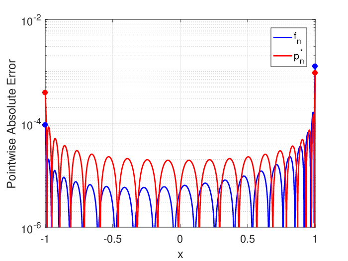
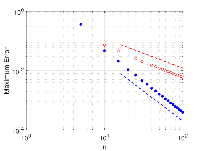
and the maximum error is always attained at one of the endpoints for large $n$ (see Figure 7). With Corollary 3.6 and (3.3), we conclude that the rate of convergence of $f_{n}$ in the maximum norm is actually one power of $n$ faster than that of $p_{n}^{*}$ whenever $\xi\in(-1,1)$ and both are the same whenever $\xi=\pm 1$ . In Figure 7 we illustrate the maximum errors and the pointwise errors of spectral differentiations using $f_{n}$ and $p_{n}^{*}$ . As expected, we see that the maximum errors of $f_{n}$ converges one power of $n$ faster than that of $p_{n}^{*}$ for $\xi\in(-1,1)$ and both converge at the same rate whenever $\xi=\pm 1$ . Moreover, concerning the pointwise errors of spectral differentiation using $f_{n}$ and $p_{n}^{*}$ , we see that Chebyshev spectral differentiations converge also faster than their best counterparts except in a small neighborhood of the singularity.

3.4 Other orthogonal projections

The error estimate of other orthogonal projections such as Legendre, Gegenbauer and Jacobi projections has attracted attention in recent years (see, e.g., [3, 18, 34, 35, 37, 38]). In [34, Figure 3] it has been observed that the error curves of Legendre projections illustrate similar character as that of Chebyshev projections. In the case of Gegenbauer and Jacobi projections, however, the situation is slightly more complicated since the errors at both endpoints may dominate the maximum error (see [35]). In the following, we restrict our attention to the case of Legendre projections and show the intrinsic connection between the error of Legendre projections and the two functions $\Psi_{\nu}^{\mathrm{C}}(x,n)$ and $\Psi_{\nu}^{\mathrm{S}}(x,n)$ defined in (1.6).

Let $f$ be the model function defined in (1.4) and let $\mathcal{P}_{n}(x)$ be its Legendre projection of degree $n$ , i.e.,

\displaystyle\mathcal{P}_{n}(x)=\sum_{k=0}^{n}a_{k}^{L}P_{k}(x),\quad a_{k}^{L}=\frac{2k+1}{2}\int_{-1}^{1}f(x)P_{k}(x)\mathrm{d}x,

(3.40)

where $P_{k}(x)$ is the Legendre polynomial of degree $k$ . By taking the Taylor series of $g(x)$ at $x=\xi$ and using [13, Equation (7.232.3)], we obtain the asymptotic behavior of the Legendre coefficients

\displaystyle a_{k}^{L}=\mathcal{E}(\alpha,\xi)\frac{\lambda_{1}(\xi)T_{k}(\xi)+\lambda_{2}(\xi)(1-\xi^{2})^{1/2}U_{k-1}(\xi)}{k^{\alpha+1/2}}+O(k^{-\alpha-3/2}),

(3.41)

where $\lambda_{j}(\xi)=(1+\xi)^{1/2}+(-1)^{j+1}(1-\xi)^{1/2}$ and

\displaystyle\mathcal{E}(\alpha,\xi)=-\sqrt{\frac{2}{\pi}}(1-\xi^{2})^{\alpha/2+1/4}\sin\left(\frac{\alpha\pi}{2}\right)\Gamma(\alpha+1)g(\xi).

On the other hand, recall from [23, Theorem 8.21.2] that

	$\displaystyle P_{k}(x)$	$\displaystyle=\sqrt{\frac{2}{\pi}}\frac{(1-x^{2})^{-1/4}}{k^{1/2}}\cos\left(\frac{2k+1}{2}\arccos(x)-\frac{\pi}{4}\right)+O(k^{-3/2})$
		$\displaystyle=\frac{(1-x^{2})^{-1/4}}{\sqrt{2\pi k}}\left[\lambda_{1}(x)T_{k}(x)+\lambda_{2}(x)(1-x^{2})^{1/2}U_{k-1}(x)\right]+O(k^{-3/2}),$		(3.42)

where the asymptotic formula on the right-hand side of (3.4) holds uniformly on the interval $[-1+\varepsilon,1-\varepsilon]$ , where $\varepsilon>0$ is small. Let us now consider the pointwise error estimate of $\mathcal{P}_{n}(x)$ and we restrict the analysis to the case where $\xi\in(-1,1)$ since the case $\xi=\pm 1$ can be treated in a similar way. Combining (3.41) and (3.4) and after some elementary calculations, we obtain for $x\in(-1,1)$ that

$\displaystyle f(x)-\mathcal{P}_{n}(x)=\frac{\mathcal{E}(\alpha,\xi)}{\sqrt{2\pi}(1-x^{2})^{1/4}}$	$\displaystyle\left[\frac{\lambda_{1}(\xi)\lambda_{1}(x)}{2}\sum_{k=n+1}^{\infty}\frac{\cos(2k\varphi_{\xi}^{+})+\cos(2k\varphi_{\xi}^{-})}{k^{\alpha+1}}\right.$
	$\displaystyle+\frac{\lambda_{1}(\xi)\lambda_{2}(x)}{2}\sum_{k=n+1}^{\infty}\frac{\sin(2k\varphi_{\xi}^{+})+\sin(2k\varphi_{\xi}^{-})}{k^{\alpha+1}}$
	$\displaystyle+\frac{\lambda_{1}(x)\lambda_{2}(\xi)}{2}\sum_{k=n+1}^{\infty}\frac{\sin(2k\varphi_{\xi}^{+})-\sin(2k\varphi_{\xi}^{-})}{k^{\alpha+1}}$	(3.43)
	$\displaystyle\left.+\frac{\lambda_{2}(x)\lambda_{2}(\xi)}{2}\sum_{k=n+1}^{\infty}\frac{\cos(2k\varphi_{\xi}^{+})-\cos(2k\varphi_{\xi}^{-})}{k^{\alpha+1}}\right]$
	$\displaystyle+O(n^{-\alpha-2}).$

Clearly, we see that the leading term of the error of $\mathcal{P}_{n}(x)$ can be represented as a linear combination of $\Psi_{\nu}^{\mathrm{C}}(x,n)$ and $\Psi_{\nu}^{\mathrm{S}}(x,n)$ . Furthermore, applying Lemma 2.2 to (3.4), we can deduce that the term inside the square bracket on the right-hand side of the last equality behaves like $O(n^{-\alpha-1})$ whenever $x$ is away from $\xi$ and behaves like $O(n^{-\alpha})$ whenever $x=\xi$ . For $x=\pm 1$ , combining the fact that $P_{k}(\pm 1)=(\pm 1)^{k}$ for all $k\in\mathbb{N}_{0}$ as well as Lemma 2.2 and (3.41) yields

	$\displaystyle f(\pm 1)-\mathcal{P}_{n}(\pm 1)$	$\displaystyle=\sum_{k=n+1}^{\infty}(\pm 1)^{k}a_{k}^{L}=\mathcal{E}(\alpha,\xi)\left(\lambda_{1}(\xi)\sum_{k=n+1}^{\infty}\frac{(\pm 1)^{k}T_{k}(\xi)}{k^{\alpha+1/2}}\right.$
		$\displaystyle~~~~~~~~~~~\left.+\lambda_{2}(\xi)\sum_{k=n+1}^{\infty}\frac{(\pm 1)^{k}(1-\xi^{2})^{1/2}U_{k-1}(\xi)}{k^{\alpha+1/2}}\right)+\cdots.$		(3.44)

We see that the leading term on the right-hand side of the last equality can also be represented by a linear combination of $\Psi_{\nu}^{\mathrm{C}}(x,n)$ and $\Psi_{\nu}^{\mathrm{S}}(x,n)$ . Combining this with Lemma 2.2 we easily obtain $f(\pm 1)-\mathcal{P}_{n}(\pm 1)=O(n^{-\alpha-1/2})$ . Hence, we conclude that the pointwise error estimate of $\mathcal{P}_{n}(x)$ is

\displaystyle|f(x)-\mathcal{P}_{n}(x)|=\left\{\begin{array}[]{ll}{\displaystyle O(n^{-\alpha})},&\hbox{if~$x=\xi$,}\\[8.0pt] {\displaystyle O(n^{-\alpha-1/2})},&\hbox{if~$x=\pm 1$,}\\[8.0pt] {\displaystyle O(n^{-\alpha-1})},&\hbox{otherwise,}\end{array}\right.

Comparing the rate of pointwise convergence of $\mathcal{P}_{n}(x)$ with $p_{n}^{*}(x)$ , we see that $\mathcal{P}_{n}(x)$ converges faster than $p_{n}^{*}(x)$ by a factor of $n$ whenever $x\in(-1,\xi)\cup(\xi,1)$ and by a factor of $n^{1/2}$ whenever $x=\pm 1$ and both $\mathcal{P}_{n}(x)$ and $p_{n}^{*}(x)$ converge at the same rate whenever $x=\xi$ , and these findings justify the error localization of Legendre projections.

Remark 3.7.

In [34] the present author has studied the optimal rates of convergence of Legendre projections in the maximum norm for analytic and piecewise analytic functions and function of the form (1.4). In the case of functions with an interior singularity, i.e., $\xi\in(-1,1)$ , it has been shown that $\mathcal{P}_{n}(x)$ and $p_{n}^{*}(x)$ converge at the same rate based on the hypothesis that the maximum error of $\mathcal{P}_{n}(x)$ is attained at $x=\xi$ . Here our pointwise error estimates in (3.4) provide a theoretical justification for this hypothesis.

Remark 3.8.

Note that we have used the uniform asymptotic expansion of Legendre polynomials in compact subsets of $(-1,1)$ in the derivation of (3.4). A similar approach for the analysis of polyharmonic-Neumann expansions was used in [2, Chapter 3].

4 Concluding remarks

We have presented a thorough analysis of the pointwise error estimate of Chebyshev spectral approximations for functions with a singularity. Our key finding is that there exists an intrinsic connection between pointwise error estimates of Chebyshev spectral approximations and the two functions $\Psi_{\nu}^{\mathrm{C}}(x,n)$ and $\Psi_{\nu}^{\mathrm{S}}(x,n)$ defined in (1.6). This connection allows us to justify rigorously the error localization of Chebyshev spectral approximations, such as why their maximum error is always attained in a small neighborhood of the singularity and why they converge faster than their best counterparts except for a small neighborhood of the singularity. We further extended the framework to Chebyshev spectral differentiations and Legendre projections and justified their error localization property using similar arguments.

Finally, we highlight several directions for future research. First, it is possible to extend the current study to more general forms of singular functions, such as

f(x)=\sum_{k=1}^{m}|x-\xi_{k}|^{\alpha_{k}}g_{k}(x),\quad f(x)=g_{0}(x)\prod_{k=1}^{m}|x-\xi_{k}|^{\alpha_{k}},

where $\{\xi_{k}\}_{k=1}^{m}\subseteq\Omega$ and $\{\alpha_{k}\}_{k=1}^{m}$ are all positive and not even integers. More precisely, the extension to the former is direct since it is a linear combination of the model function (1.4). The extension to the latter is also applicable since it can also be decomposed into a linear combination of the model function (1.4) by introducing neutralizers (see [30, Equation (4.17)]). Second, we have shown that Chebyshev spectral differentiations converge faster than their best counterparts except in a neighborhood of the singularity and, in the particular case of functions with an interior singularity, they converge even faster than their best counterparts in the maximum norm. Note that spectral differentiations are widely used in the context of spectral methods, it is of great interest to extend the study to more general settings, such as Gegenbauer and Jacobi spectral differentiations.

Acknowledgements

This work was supported by National Natural Science Foundation of China under grant number 11671160. The author would like to thank Prof. Nick Trefethen for his suggestions that improved the presentation of the paper. He would also like to thank Prof. Chengming Huang for several stimulating discussions and the anonymous referee for helpful comments on this work.

References

[1] B. Adcock, Multivariate modified Fourier series and application to boundary value problems, Numer. Math., 115(4):511-552, 2010.
[2] B. Adcock, Modified Fourier expansions: theory, construction and applications, PhD Thesis, University of Cambridge, 2010.
[3] I. Babuška and H. Hakula, Pointwise error estimate of the Legendre expansion: The known and unknown features, Comput. Methods Appl. Mech. Engrg., 345(1):748–773, 2019.
[4] J. P. Berrut and L. N. Trefethen, Barycentric Lagrange interpolation, SIAM Rev., 46(3):501–517, 2004.
[5] S. Bernstein, Sur la meilleure approximation de $|x|$ par des polynômes de degrés donnés, Acta Math., 37:1–57, 1913.
[6] S. Bernstein, Sur la meilleure approximation de $|x|^{p}$ par des polynômes de degrés très élevés, Izv. Akad. Nauk SSSR Ser. Mat., 2(2):169–190, 1938.
[7] J. P. Boyd, Chebyshev and Fourier Spectral Methods, 2nd edition, Dover Publications Inc., 2000.
[8] J. P. Boyd, Finding the zeros of a univariate equation: proxy rootfinders, Chebyshev interpolation, and the companion matrix, SIAM Rev., 55(2):375–396, 2013.
[9] H. Brunner, Collocation Methods for Volterra Integral and Related Functional Differential Equations, Cambridge University Press, 2004.
[10] C. Canuto, M. Y. Hussaini, A. Quarteroni and T. A. Zang, Spectral Methods: Fundamentals in Single Domains, Springer, 2006.
[11] T. A. Driscoll, N. Hale and L. N. Trefethen, Chebfun Guide, Pafnuty Pulications, Oxford, 2014; see also www.chebfun.org.
[12] C. Ferreira and J. L. López, Asymptotic expansions of the Hurwitz-Lerch zeta function, J. Math. Anal. Appl., 298(1):210–224, 2004.
[13] I. S. Gradshteyn and I. M. Ryzhik, Table of Integrals, Series, and Products, Seventh Edition, Academic Press, 2007.
[14] N. J. Higham, The numerical stability of barycentric Lagrange interpolation, IMA J. Numer. Anal., 24(4):547–556, 2004.
[15] A. Iserles and S. P. Nørsett, From high oscillation to rapid approximation I: modified Fourier expansions, IMA J. Numer. Anal., 28(4):862-887, 2008.
[16] M. Kzaz, Asymptotic expansion of Fourier coefficients associated to functions with low continuity, J. Comput. Appl. Math., 114(2):217–230, 2000.
[17] R.-C. Li, Near optimality of Chebyshev interpolation for elementary function computations, IEEE Trans. Comput., 53(6):678–687, 2004.
[18] W.-J. Liu, L.-L. Wang and B.-Y. Wu, Optimal error estimates for Legendre expansions of singular functions with fractional derivatives of bounded variation, Adv. Comput. Math., 47:79, 2021.
[19] J. C. Mason and D. C. Handscomb, Chebyshev Polynomials, Chapman and Hall/CRC, Boca Raton, 2003.
[20] F. W. J. Olver, D. W. Lozier, R. F. Boisvert and C. W. Clark, NIST Handbook of Mathematical Functions, Cambridge University Press, 2010.
[21] S. Olver, On the convergence rate of a modified Fourier series, Math. Comp., 78(267):1629-1645, 2009.
[22] T. J. Rivlin, Chebyshev Polynomials: From Approximation theory to Algebra & Number Theory, Second Edition, Dover Publications, Inc. Mineola, New York, 2020.
[23] G. Szegő, Orthogonal Polynomials, Vol. 23, American Mathematical Society, 1939.
[24] J. Shen, T. Tang and L.-L. Wang, Spectral Methods: Algorithms, Analysis and Applications, Springer, Heidelberg, 2011.
[25] A. F. Timan, Theory of Approximation of Functions of a Real Variable, The Machillan Company, New York, 1963.
[26] L. N. Trefethen, Spectral Methods in Matlab, SIAM, Philadelphia, 2000.
[27] L. N. Trefethen, Is Gauss quadrature better than Clenshaw-Curtis? SIAM Rev., 50(1):67–87, 2008.
[28] L. N. Trefethen, Six myths of polynomial interpolation and quadrature, Maths. Today, 47:184–188, 2011.
[29] L. N. Trefethen, Approximation Theory and Approximation Practice, SIAM, Extended Edition, 2020.
[30] P. D. Tuan and D. Elliott, Coefficients in series expansions for certain classes of functions, Math. Comp., 26(117):213–232, 1972.
[31] R. S. Varga and A. J. Carpenter, On the Bernstein conjecture in approximation theory, Constr. Approx., 1(1):333–348, 1985.
[32] L. B. Wahlbin, Superconvergence in Galerkin Finite Element Methods, Springer-Verlag, Berlin, 1995.
[33] H.-Y. Wang, On the convergence rate of Clenshaw-Curtis quadrature for integrals with algebraic endpoint singularities, J. Comput. Appl. Math., 333:87–98, 2018.
[34] H.-Y. Wang, How much faster does the best polynomial approximation converge than Legendre projection?, Numer. Math., 147(2):481–503, 2021.
[35] H.-Y. Wang, Optimal rates of convergence and error localization of Gegenbauer projections, IMA J. Numer. Anal., drac047, 2022.
[36] L.-L. Wang, X.-D. Zhao and Z.-M. Zhang, Superconvergence of Jacobi-Gauss-type spectral interpolation, J. Sci. Comput., 59(3):667–687, 2014.
[37] S.-H. Xiang and G.-D. Liu, Optimal decay rates on the asymptotics of orthogonal polynomial expansions for functions of limited regularities, Numer. Math., 145(1):117–148, 2020.
[38] S.-H. Xiang, D.-S. Kong, G.-D. Liu and L.-L. Wang, Pointwise error estimates and local superconvergence of Jacobi expansions, private communication, 2021.
[39] Z.-M. Zhang, Superconvergence points of polynomial spectral interpolation, SIAM J. Numer. Anal., 50(6):2966–2985, 2012.