Generating Relevant and Coherent Dialogue Responses using Self-separated Conditional Variational AutoEncoders
Abstract
Conditional Variational AutoEncoder (CVAE) effectively increases the diversity and informativeness of responses in open-ended dialogue generation tasks through enriching the context vector with sampled latent variables. However, due to the inherent one-to-many and many-to-one phenomena in human dialogues, the sampled latent variables may not correctly reflect the contexts’ semantics, leading to irrelevant and incoherent generated responses. To resolve this problem, we propose Self-separated Conditional Variational AutoEncoder (abbreviated as SepaCVAE) that introduces group information to regularize the latent variables, which enhances CVAE by improving the responses’ relevance and coherence while maintaining their diversity and informativeness. SepaCVAE actively divides the input data into groups, and then widens the absolute difference between data pairs from distinct groups, while narrowing the relative distance between data pairs in the same group. Empirical results from automatic evaluation and detailed analysis demonstrate that SepaCVAE can significantly boost responses in well-established open-domain dialogue datasets.
1 Introduction
When conversing with a human user, an open-domain dialogue system is expected to generate human-like responses – responses that not only are diverse and informative, but also contain relevant and cohesive information that correctly addresses the context dialogue. Through using sampled latent variables, Conditional Variational AutoEncoders (CVAE) are powerful tools to ensure diversity and informativeness of the generated responses (Bowman et al. 2016; Serban et al. 2017; Shen et al. 2017; Zhao et al. 2017; Chen et al. 2018). Yet, it is challenging for a CVAE-based dialogue generation model to keep the responses relevant and coherent. The challenge arises as human dialogues inherently exhibit the one-to-many and many-to-one phenomena (Csaky et al. 2019), meaning that the same context could lead to very different responses, and different contexts could lead to the same response, respectively. As a result, the latent variables sampled by CVAE often fail to capture the correct contextual semantics, as shown in Fig. 1, leaving open the possibility that similar contexts producing drastically different latent variables. This has two particular drawbacks:
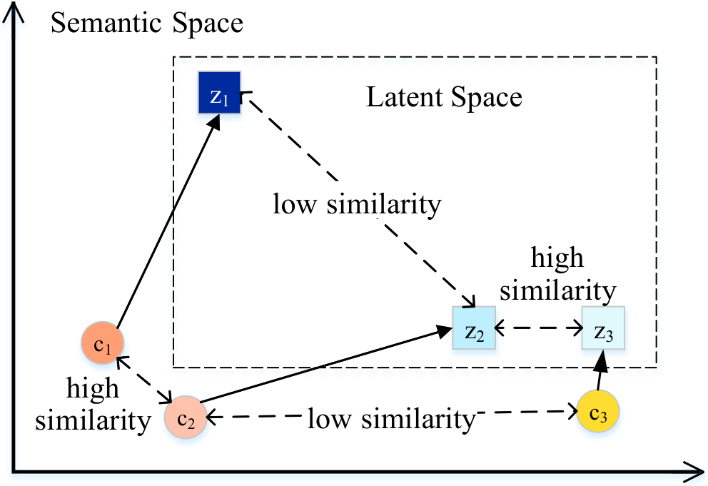
First, the discrepancy between latent variables could lead to irrelevant and incoherent generated responses. Different latent variables in a continuous latent space correspond to different responses (Bowman et al. 2016). As dissimilar latent variables may be sampled for similar contexts, the generated responses for contexts in the test set could be drastically different from responses to similar contexts in the training set. For instance, given a context “Everything about this movie is awesome!”, a standard CVAE may generate response as dissimilar as“Smartphones of the best games!.” and “Caves would never say yes, but I’d love to know.” (Gao et al. 2019). Thus this approach sacrifices too much relevance and coherence for diversity and informativeness.
Second, the disparity between contexts and latent variables hurts model generalizability. Model generalizability is often evaluated using a separate dataset taken from a similar distribution as the training set (e.g., a validation or a noisy version of the training set). High generalizability is indicated if the model can transfer favourable abilities from the training set to this second dataset, in the sense that it produces consistent responses between similar contexts across the two datasets. This suggests that the model has acquired certain semantic relations between sentences from the training set. However, if the sampled latent variable departs significantly from the contextual semantics, the model may perform quite differently on the second dataset from the training set.
To address these drawbacks, we propose a novel model, namely Self-Separated Conditional Variational Autoencoder (SepaCVAE). SepaCVAE proactively partitions the input data into a number of groups, and then widens the absolute differences between data pairs across different groups while narrowing the relative distance between data pairs within the same group. In this way, SepaCVAE aims to put the contexts that sample similar latent variables into the same groups, thereby regularizing the latent variables. The design of SepaCVAEinvolves three components that are built on top of standard CVAE. First, inspired from image augmentation, we propose a dialogue augmentation method to partition data without any prior knowledge. For this, we construct orthogonal vectors to classify data into groups, which retain the original semantic relationships of data within a group. We directly enlarge the semantic distance of the data across different groups. Then, we propose a gradient blocking algorithm to select the most suitable group for each data according to gains obtained from different groups. Here, the gains are evaluated using reconstruction loss. Finally, inspired from the contrastive learning paradigm (Cai et al. 2020; Chen et al. 2020a; Chen et al. 2020b; Mitrovic et al. 2020), we propose relationship enhancement to increase similarity between the representations of data within the same group, and differentiate the representations of data between different groups.
Contributions: Our first contribution is a theoretical analysis on why sampled latent variables fail to reflect the contexts’ semantics. The next contribution lies in the proposal of SepaCVAE to overcome issues of irrelevant and incoherent responses caused by standard CVAE. Our third contribution involves a series of experiments. The results show that our SepaCVAE can generate more relevant and coherent responses compared to existing methods.
2 Related work
2.1 Dialogue models
Open-domain dialogue generation is a challenging task in natural language processing. Early dialogue models (Shang et al. 2015; Sordoni et al. 2015b) often tend to generate dull responses. To improve the quality of these responses, two pathways have been adopted: one is to introduce external semantic information, such as dialogue history (Sordoni et al. 2015a; Serban et al. 2016), topic (Xing et al. 2017), sentiment (Huber et al. 2018), knowledge (Ghazvininejad et al. 2018), persona-style (Li et al. 2016c), and other information (Li et al. 2016a; Wang et al. 2017; Baheti et al. 2018; Feng et al. 2020b). The other is through more complex models or frameworks, such as attention mechanisms (Bahdanau et al. 2015; Luong et al. 2015), reinforcement learning (RL) (Li et al. 2016d; Zhang et al. 2018a; Liu et al. 2020), generative adversarial network (GAN) (Yu et al. 2017; Li et al. 2017a; Zhang et al. 2018b; Feng et al. 2020a), and variational reasoning (Bowman et al. 2016; Serban et al. 2017; Shen et al. 2017; Zhao et al. 2017; Chen et al. 2018).
CVAE models are conversational models that are based on variational reasoning. Many existing CVAE models have achieved state-of-the-art performance by generating diverse and informative responses. Moreover, as opposed to methods that introduce external semantic information, CVAE models use latent variables to represent such information. Hence they can be applied when external information is not available. Comparing with the models based on RL or GAN, CVAE models are simpler and can be easily trained. In addition, CVAE models can be enhanced by methods that use RL or GAN as generators to further improve their performances.
However, empirical evidences (Gao et al. 2019; Gu et al. 2019) have indicated that while the use of latent variables may make the generated responses more diverse and informative, it could also reduce relevance and coherence. To alleviate this apparent issue, CVAE models have been used in combination with external information such as persona information, dialogue history and dialogue act (Shen et al. 2017; Serban et al. 2017; Zhao et al. 2017). However, simply borrowing external information is not sufficient to resolve the one-to-many issue, especially when the amount of data is very large. No existing model resolves the core issue of the problem, that is, the latent variable inherits little semantic information from the context sentence, a consequence of the inherent one-to-many and many-to-one phenomena of human conversations. To address this issue, we propose the SepaCVAE model which trains latent variables that inherit contextual semantics.
2.2 Self-supervised method used in dialogue generation task
Recently, self-supervised methods such as contrastive learning – popularized in computer vision Chen et al. 2020a; Chen et al. 2020b – are drawing increasing attention in NLP (Wu et al. 2019; Clark et al. 2020; Cai et al. 2020). Generally speaking, the major issue with applying contrastive learning is how positive and negative examples are constructed. Many existing work explore ways to design reasonable pairs of positive and negative examples to accurately capture the semantic relations of these pairs, so that the obtained representation can be better-used on downstream tasks.
3 Problem formulation
The problem with the standard CVAE model lies in that the sampled latent variables may not accurately reflect the contextual semantics due to the apparent one-to-many (one context may correspond to many responses) and many-to-one (many contexts may also correspond to one response) phenomena. This leads to irrelevant and incoherent responses, and harms model generalizability. Our aim is to adapt sampled latent variables to capture the contextual semantics, so that the effects of these phenomena are neutralized. This will in turn be helpful to generate relevant and coherent responses. With this goal, we focus on single-turn dialogue datasets where the one-to-many situations appear more frequently than multi-turn dialogue datasets.
3.1 Preconditions
This section formally analyzes the many-to-one and one-to-many phenomena and we present several important assumptions and contextual information (i.e., preconditions) for the CVAE model.
Notations: and are parameters of CVAE’s recognition network and prior network, respectively; represents the condition information, and represent the generation target, and represents the latent variable.
Precondition 1: Bowman et al. 2016 confirmed that the latent space is continuous; the latent variable is highly correlated with the target data , meaning that different will reconstruct different .
Precondition 2: CVAE has a recognition network and a prior network to approximate the true posterior distribution and prior distribution , respectively. These distributions are assumed to follow the Gaussian distribution, e.g., .
Precondition 3: To efficiently train a CVAE model, the Stochastic Gradient Variational Bayes (SGVB) framework (Sohn et al. 2015; Yan et al. 2016; Kingma and Welling 2014) is adopted which aims to maximize the variational lower bound of the conditional log likelihood:
| (1) |
where represents Kullback–Leibler divergence. During training, the of will get smaller and smaller, and the of will get closer and closer to that corresponding to , which aims to stabilize the and make it converge.
3.2 Demonstrating the existence of the problem

We use Fig. 2 to illustrate the impact of one-to-many phenomenon and many-to-one phenomenon on a trained standard CVAE model. Consider the situation in Fig. 2(a) where the context has two different responses and . By Precondition 2, we assume two approximate posterior distributions , and one approximate prior distribution . By Precondition 3, during training, and will get closer to the latent variables that could be reconstructed to and , respectively. By Precondition 1, as is different from , should also be different from . Otherwise, the latent variables sampled from and tend to be the same, making these latent variables irrelevant to the responses. This leads to the vanishing latent variable problem (Bowman et al. 2016). Therefore, and cannot be the same, and their discrepancy can be considered stable; only in this way we can ensure one-to-one correspondence between latent variables and responses. From Precondition 3, it is easy to see that is only affected by . Hence, we ignore in Eq. (3.1) and use to analyze the trend of during training. Considering Fig. 2(a) where of and equals to . We provide details of the computation in Appendix A. The formulation can then be simplified as:
Hence, we can compute and that minimizes the above using Lagrange multiplier:
The derivation above provides insights on the problem caused by the one-to-many phenomena in Fig. 2(a): After training, the prior conditional probability , which will be used in inference. If the difference between and widens, the difference between and will also widen and will become further away from and . During inference, the latent variables sampled from have a high probability to differ from those sampled from and . These latent variables will introduce irrelevant information and contribute to the generation of irrelevant responses. In addition, as one response may correspond to different contexts and , as shown in Fig. 2(b), and tend to be the same, which contributes to the phenomenon that different context could sample similar latent variables. In a word, similar contexts could correspond to different latent variables and different contexts could correspond to similar latent variables, which explains why the latent variables can not accurately reflect the contexts’ semantics.
4 Method
In this section, we introduce in detail the proposed SepaCVAE model and its three key components, dialogue augmentation, gradient blocking, and relationship enhancement.
4.1 Self-Separated CVAE

As shown in Fig. 3, SepaCVAE uses to separate the contexts into different groups. For the one-to-many phenomenon, the contexts in different groups will have different prior distributions , which is easily affected by the different posterior distributions. As for the many-to-one phenomenon, SepaCVAE makes the contexts generate latent variables related to the response only when it contains group information . The other group would help the contexts to align with the other latent variables.
4.2 Dialogue augmentation
In SepaCVAE, we first propose dialogue augmentation (see Algorithm 1), which designs a group of orthogonal vectors to separate the contexts into different groups. These vectors are called group information.
In SepaCVAE, we apply Algorithm 1 to extend each dialogue pair to before feeding them to start training. If different contexts have the same added, then these contexts belong to the same group. In this way, all contexts will keep a certain relationship within the same group. In this work, the value is set to 8. Since we use to replace the original , the variational lower bound of SepaCVAE is re-written as:
| (2) |
4.3 Gradient blocking
Before the gradient back-propagation, we propose gradient blocking (see Algorithm 2 in Appendix B for implementation details) to filter the gradients. Since we extend the dialogue pair to , if we optimize the model through all calculated gradients, would be regarded as noise. Therefore, We choose the largest variational lower bound that is calculated through the dialogue pair with the positive group information , which can be represented as (3):
| (3) |
For each , we only pass to optimize the model.
4.4 Relationship enhancement
Through dialogue augmentation and gradient blocking, the positive for each dialogue pair is captured. We then propose relationship enhancement, which is inspired from contrastive learning, to adjust the separated results. Those responses under the same are considered to be in the same group, and thus can be seen as positive samples; similarly, those responses under different are seen as negative samples. From the perspective of contrastive learning, we design a relationship-enhancement-loss named to help our model achieve the representation learning:
| (4) | ||||
where represents the embedded generated response, represents our model’ encoder, means the number of positive samples, and means the number of negative samples.
In addition, we introduce an MLP to predict based on vector representation of the generated response . We therefore define :
| (5) |
Overall, SepaCVAE is trained by maximizing:
| (6) |
Quoting the KL annealing trick (Bowman et al. 2016), increases linearly from 0 to 1 in the first 10,000 batches.
5 Experiments
5.1 Dataset
We use two public dialogue datasets in our experiments, and change them as single-turn dialog data. The first dataset, named DailyDialog Li et al. 2017b, consists of dialogues that resemble human daily communication. The second dataset, named OpenSubtitles Tiedemann 2009, includes a large collection of conversations converted from movie transcripts in English.
5.2 Data pre-processing
In this work, we extract single-turn dialogues from two dialogue datasets, DailyDialog and OpenSubtitles. From a multi-turn dialogue , we can extract single-turn dialogues , where represents an utterance. As discussed above, compared with multi-turn dialogue dataset the single-turn dialogue dataset contains a more serious one-to-many problem. Therefore, using the single-turn dialogue dataset for experimentations can highlight the problem of general CVAE model and reflect the effect of our method.
We utilize 300-dimensional GloVe embeddings Pennington et al. 2014 to represent these dialogues in vectors. Since the tokens in GloVe do not cover all tokens in DailyDialog and OpenSubtitles datasets, we extract the token-list of GloVe to filter these datasets. Table 1 lists key statistics of the dataset after processing.
| dataset name | vocab | train | valid | test |
|---|---|---|---|---|
| DailyDialog | 10,064 | 18,406 | 2,008 | 988 |
| OpenSubtitles | 87,840 | 5M | 100K | 50K |
In addition, we count the one-to-many samples of both datasets and found that 408 contexts in DailyDialog and 90,149 contexts in OpenSubtitles have multiple responses. In particular, a context in OpenSubtitles has a maximum of 623 responses, while a context in DailyDialog has a maximum of 29 responses, which shows that the one-to-many phenomenon is more prevalent in OpenSubtitles dataset.
5.3 Automatic evaluation metrics
We use ppl (Neubig 2017), response length and distinct-n (Li et al. 2016b) to evaluate the diversity of generated responses. We also use BLEU (Papineni et al. 2002) to evaluate the degree of the word-overlap between generated responses and ground truth. Moreover, we use Embedding Average (Average) (Liu et al. 2016)) to evaluate the semantic relationship of generated responses and ground-truth responses. Finally, we introduce the coherence (Xu et al. 2018b) to assess the coherence between contexts and generated responses.
5.4 Human evaluation
We conduct human evaluation to further evaluate our model and baseline models. Following the work of Li et al. 2017a; Xu et al. 2018a, we randomly extract 200 samples from the test sets of the two dialogue datasets, respectively. Each sample contains one context and the response generated by different models. Three annotators are invited to rank the generated responses with respect to three aspects: diversity, relevance and fluency. Ties are allowed. Diversity indicates how much the generated response provides specific information, rather than generic and repeated information. Relevance means how likely the generated response is relevant to the context. Fluency specifies how likely the generated response is produced by human.
5.5 Baseline models
Our baseline models include sequence-to-sequence (Seq2Seq) model, CVAE model, and cluster-CVAE model. They are all implemented based on a 2-layer GRU kgCVAE model Zhao et al. 2017. The cluster-CVAE model represents that kgCVAE utilize the cluster results as the knowledge. We employ three cluster methods, i.e. K-means(K), Spectral(S), Agglomerative(A).
5.6 Training details
| mode | ppl | distinct-1 | distinct-2 | length | BLEU-1 | Average | coherence |
|---|---|---|---|---|---|---|---|
| Seq2Seq | 42.9.18 | 0.033.01 | 0.119.02 | 9.1.22 | 0.386.00 | 0.858.00 | 0.763.00 |
| CVAE | 13.3.09 | 0.074.00 | 0.407.01 | 11.3.33 | 0.405.01 | 0.853.00 | 0.763.00 |
| CVAE+BOW | 13.0.30 | 0.078.00 | 0.415.01 | 11.4.21 | 0.402.01 | 0.855.00 | 0.762.00 |
| K-CVAE+BOW | 13.1.11 | 0.074.00 | 0.406.01 | 11.5.14 | 0.424.00 | 0.868.00 | 0.766.00 |
| S-CVAE+BOW | 12.9.12 | 0.075.00 | 0.414.01 | 11.5.17 | 0.426.01 | 0.867.00 | 0.765.00 |
| A-CVAE+BOW | 13.0.22 | 0.076.00 | 0.418.02 | 11.6.11 | 0.418.00 | 0.863.00 | 0.765.00 |
| SepaCVAE | 9.8.17 | 0.078.00 | 0.504.01 | 11.5.10 | 0.461.00 | 0.862.00 | 0.767.00 |
| Seq2Seq | 45.9.13 | 0.002.00 | 0.010.00 | 11.8.81 | 0.236.04 | 0.465.08 | 0.281.05 |
| CVAE+BOW | 12.2.17 | 0.005.00 | 0.095.00 | 13.1.26 | 0.172.02 | 0.285.04 | 0.195.03 |
| K-CVAE+BOW | 12.1.20 | 0.006.00 | 0.098.00 | 13.1.10 | 0.203.02 | 0.311.06 | 0.200.05 |
| SepaCVAE | 2.0.06 | 0.016.00 | 0.282.01 | 12.6.11 | 0.417.00 | 0.836.01 | 0.707.01 |
| mode | distinct-1 | distinct-2 | length | BLEU-2 | BLEU-3 | Average | coherence |
|---|---|---|---|---|---|---|---|
| Seq2Seq | 0.054.01 | 0.180.03 | 9.0.32 | 0.300.01 | 0.247.00 | 0.856.00 | 0.756.01 |
| CVAE | 0.106.00 | 0.499.01 | 11.3.25 | 0.324.01 | 0.272.01 | 0.854.00 | 0.756.00 |
| CVAE+BOW | 0.114.00 | 0.514.01 | 11.2.13 | 0.326.01 | 0.274.01 | 0.856.00 | 0.755.00 |
| K-CVAE+BOW | 0.108.00 | 0.501.02 | 11.6.16 | 0.342.01 | 0.287.00 | 0.869.00 | 0.759.00 |
| S-CVAE+BOW | 0.110.00 | 0.511.01 | 11.4.19 | 0.339.00 | 0.284.00 | 0.867.00 | 0.758.00 |
| A-CVAE+BOW | 0.111.01 | 0.509.02 | 11.5.16 | 0.331.00 | 0.278.00 | 0.862.00 | 0.757.00 |
| SepaCVAE | 0.082.00 | 0.471.01 | 17.9.57 | 0.409.01 | 0.350.01 | 0.877.00 | 0.809.00 |
| Seq2Seq | 0.003.00 | 0.015.00 | 11.8.82 | 0.193.03 | 0.163.03 | 0.465.08 | 0.281.05 |
| CVAE+BOW | 0.009.00 | 0.131.00 | 13.1.24 | 0.144.02 | 0.123.02 | 0.285.04 | 0.195.03 |
| K-CVAE+BOW | 0.010.00 | 0.135.00 | 13.1.10 | 0.169.02 | 0.144.01 | 0.308.06 | 0.198.05 |
| SepaCVAE | 0.025.00 | 0.330.03 | 13.5.58 | 0.326.01 | 0.276.01 | 0.807.02 | 0.677.01 |
For a fair comparison among all models, we utilized 300-dimensional GloVe embeddings as the word embedding matrix. The numbers of hidden nodes are all set to 300. The parameter is set to 25. We set the batch sizes to 64 and 32 for DailyDialog and OpenSubtitles datasets, respectively. Adam is utilized for optimization. The parameter is set to 0.001. We train all models in 50 epochs on a RTX 2080Ti GPU card with Tensorflow, and save the generated responses when the ppl reaching minimum. Greedy search is used to generate responses for evaluation.
6 Results and Discussion
6.1 Automatic evaluation results
Table 2 and Table 3 report the automatic evaluation results of SepaCVAE and baseline models on validation and test data of both two datasets, respectively. For the validation stage, we first select and save the positive group information () for each context, and then generate responses under this . For the test data where no ground truth response is available to select the positive group information, we first generate responses for each context through group information, and then choose the most possible generated response through calculating the cosine score between the generated responses and context. Both generated responses and contexts are input into SepaCVAE’s encoder to obtain the vector representations.
Spectral and Agglomerative cluster methods would not work well under the large-scale dataset (i.e. OpenSubtitles), and the general CVAE model suffers from the vanishing latent variable problem while training on such dataset. Therefore, we remove the results of S-CVAE+BOW, A-CVAE+BOW and CVAE on Table 2 and Table 3.
As shown in Table 2 and Table 3, the results on large-scale dataset (OpenSubtitles) are better than that on small dataset (DailyDialog), that is, the results on OpenSubtitles show an obvious pattern that verifies our hypothesis. On both validation and test data of OpenSubtitles, CVAE and K-CVAE achieve better performance on diversity metric (distinct) but worse performance on relevant metrics (i.e. BLEU, Average and coherence) than Seq2Seq model. Moreover, our proposed SepaCVAE outperforms all baseline models in terms of all metrics with statistical significance. However, the results obtained on the DailyDialog dataset do not show a clear pattern. For DailyDialog’s validation data, SepaCVAE achieves good performance on diversity but on relevance the results is unimpressive. On the other hand, for test data, SepaCVAE achieves good performance on relevance but generally poor results on diversity. We believe that the reason for this phenomenon is related to the level of prevalence of the one-to-many phenomenon in the dataset. For instance, only 66,260 contexts have multiple responses among the 90,149 contexts on the OpenSubtitles that was added the cluster results. Moreover, one context has a maximum of 296 responses, which amounts to almost half of 623. Since the DailyDialog dataset is very small and contains few samples that we focus on, which cause the not specific tendency on its results. In a word, the evaluation results illustrate the effectiveness of SepaCVAE in terms of improving the relevance and coherence of responses.
6.2 Human evaluation results
| model | diversity | relevance | fluency |
|---|---|---|---|
| Seq2Seq | 3.64 | 3.12 | 2.16 |
| CVAE+BOW | 3.16 | 3.58 | 3.42 |
| K-CVAE+BOW | 3.27 | 3.71 | 3.49 |
| SepaCVAE | 2.11 | 2.95 | 3.49 |
| Ground-truth | 1.88 | 1.02 | 1.00 |
| Seq2Seq | 3.12 | 3.11 | 3.24 |
| CVAE+BOW | 2.69 | 2.98 | 3.05 |
| K-CVAE+BOW | 2.59 | 3.53 | 3.72 |
| SepaCVAE | 2.57 | 2.36 | 2.25 |
| Ground-truth | 2.49 | 1.12 | 1.02 |
The results of the human evaluation are shown in Table 4. To evaluate the consistency of the ranking results assessed by three annotators, we use Pearson’s correlation coefficient. This coefficient is 0.22 on diversity, 0.63 on relevance, and 0.70 on fluency, with and below 0.001, which indicates high correlation and agreement. Similarly with the automatic evaluation results in Table 3, this result shows that our SepaCVAE significantly outperforms baselines in term of relevance and diversity. Except the ground-truth responses, our SepaCVAE achieve the best scores of relevance and diversity metrics. The fluency result of SepaCVAE on the DailyDialog dataset is slightly worse than that of baselines, which is mainly due to the length of responses generated by SepaCVAE is almost two times than that of baselines (see Table 3). When the response lengths are similar on the Opensubtitles dataset, SepaCVAE could also achieve the best fluency score.
6.3 Effectiveness analysis
.
We further analyze the effectiveness of SepaCVAE on regularizing latent variables. For the contexts in the validation data of DailyDialog dataset, we collect their generated responses and the sampled latent variables of both SepaCVAE and baseline models on the first 2,500 batches. Then we calculate the average inner-group distance and the average inter-group distance for each context based on jointly vector representations (concatenating the context vector and the latent variable). All distances are calculated by cosine scores, and the higher the distance, the greater the similarity.
For each context, SepaCVAE outputs a positive group information , which is used to distinguish whether other contexts are in the same group. As for the standard CVAE, we set a threshold of the cosine score to replace the group information. In this work, the threshold is set to 0.9. Finally, we take the average of all contexts’ inner-group distance results and inter-group distance results as inner-dis. and inter-dis. of each batch, which are shown in Fig. 4. SepaCVAE achieves significantly higher inner-dis. than baseline (standard CVAE) model, while the inter-dis. are similar. Meanwhile, our method also gets the similar average distance of all jointly vectors with the standard CVAE.
In addition, past studies conjecture that the posterior sampled from the recognition network should cluster the responses into meaningful groups that correlate with the knowledge. Fig. 5 visualizes the posterior of responses in the validation data of DailyDialog dataset in 2D space using t-SNE (van der Maaten and Hinton 2008). We found that the learned latent space of our SepaCVAE is more correlated with the group information. These results demonstrate that SepaCVAE can effectively regularize latent variables.
6.4 Case study
| samples in training dataset | |
|---|---|
| context | would you like to have dinner with me tonight? |
| true response 1 | oh, that sounds great! |
| true response 2 | sorry, i have to work overtime. |
| sample in validation dataset | |
| similar context | i would always be ready to go shopping with you! should we talk about other basics? |
| Seq2Seq | sure. we will go to the movies. |
| CVAE | i’m not interested in your are not a good thing! |
| CVAE+BOW | it will smell and better if whatever, whatever. |
| SepaCVAE | sure, it will be happy, mary, most music is well. |
| sample in test dataset | |
| similar context | me, too. do you want to go out to celebrate my good news? |
| Seq2Seq | yes, i’m going to go to the beach. |
| CVAE | it really really talking from the street. mom. |
| CVAE+BOW | there may live in the rocks, please. |
| SepaCVAE | sure. i go with my parents. i am so excited about these friends! |
We collected the generated responses of contexts in validation and test set, which are similar to the training set, and showed a sample in Table 4. The context in training set has two contradictory responses. As we analyzed, the standard CVAE and CVAE+BOW generated irrelevant and incoherent response for the similar context in validation and test set. In contrast, our SepaCVAE outputted sure, it will be happy and sure. i go with my parents are more relevant and coherent than the response generated by baselines, and it also similar with the true response 1 (oh, that sounds great!), which means the SepaCVAE is able to handle the one-to-many situation.
7 Conclusion
In this paper, we theoretically prove that latent variables hardly reflect the semantics of contexts due to the one-to-many and many-to-one phenomena of dialogues. For the standard CVAE model, these issues lead to irrelevant and incoherent responses during the validation or test stage, and also damaging the generalization performance. To address these problems, we proposed the SepaCVAE model. There are three main technical novelties of SepaCVAE: dialogue augmentation, gradient blocking, and relationship enhancement, which enable the latent variables to reflect semantic relationships between contexts. As demonstrated in the experimental results, SepaCVAE could get the best performance for large-scale dataset.
Acknowledgements
We would like to thank the anonymous reviewers for their constructive comments. This research is supported by Beijing Natural Science Foundation (No. L181010 and 4172054), National Key R&D Program of China (No. 2016YFB0801100). Kan Li is the corresponding author.
References
- Bahdanau et al. (2015) Dzmitry Bahdanau, Kyunghyun Cho, and Yoshua Bengio. 2015. Neural machine translation by jointly learning to align and translate. In ICLR.
- Baheti et al. (2018) Ashutosh Baheti, Alan Ritter, Jiwei Li, and Bill Dolan. 2018. Generating more interesting responses in neural conversation models with distributional constraints. In EMNLP, pages 3970–3980. Association for Computational Linguistics.
- Bowman et al. (2016) Samuel R. Bowman, Luke Vilnis, Oriol Vinyals, Andrew M. Dai, Rafal Józefowicz, and Samy Bengio. 2016. Generating sentences from a continuous space. In CoNLL, pages 10–21. ACL.
- Cai et al. (2020) Hengyi Cai, Hongshen Chen, Yonghao Song, Zhuoye Ding, Yongjun Bao, Weipeng Yan, and Xiaofang Zhao. 2020. Group-wise contrastive learning for neural dialogue generation. In EMNLP, pages 793–802. Association for Computational Linguistics.
- Chen et al. (2018) Hongshen Chen, Zhaochun Ren, Jiliang Tang, Yihong Eric Zhao, and Dawei Yin. 2018. Hierarchical variational memory network for dialogue generation. In WWW, pages 1653–1662. ACM.
- Chen et al. (2020a) Ting Chen, Simon Kornblith, Mohammad Norouzi, and Geoffrey E. Hinton. 2020a. A simple framework for contrastive learning of visual representations. In ICML, volume 119 of Proceedings of Machine Learning Research, pages 1597–1607. PMLR.
- Chen et al. (2020b) Xinlei Chen, Haoqi Fan, Ross B. Girshick, and Kaiming He. 2020b. Improved baselines with momentum contrastive learning. CoRR, abs/2003.04297.
- Clark et al. (2020) Kevin Clark, Minh-Thang Luong, Quoc V. Le, and Christopher D. Manning. 2020. ELECTRA: pre-training text encoders as discriminators rather than generators. In ICLR. OpenReview.net.
- Csaky et al. (2019) Richard Csaky, Patrik Purgai, and Gábor Recski. 2019. Improving neural conversational models with entropy-based data filtering. In ACL (1), pages 5650–5669. Association for Computational Linguistics.
- Feng et al. (2020a) Shaoxiong Feng, Hongshen Chen, Kan Li, and Dawei Yin. 2020a. Posterior-gan: Towards informative and coherent response generation with posterior generative adversarial network. In AAAI, pages 7708–7715. AAAI Press.
- Feng et al. (2020b) Shaoxiong Feng, Xuancheng Ren, Hongshen Chen, Bin Sun, Kan Li, and Xu Sun. 2020b. Regularizing dialogue generation by imitating implicit scenarios. In EMNLP, pages 6592–6604. Association for Computational Linguistics.
- Gao et al. (2019) Xiang Gao, Sungjin Lee, Yizhe Zhang, Chris Brockett, Michel Galley, Jianfeng Gao, and Bill Dolan. 2019. Jointly optimizing diversity and relevance in neural response generation. In NAACL-HLT (1), pages 1229–1238. Association for Computational Linguistics.
- Ghazvininejad et al. (2018) Marjan Ghazvininejad, Chris Brockett, Ming-Wei Chang, Bill Dolan, Jianfeng Gao, Wen-tau Yih, and Michel Galley. 2018. A knowledge-grounded neural conversation model. In AAAI, pages 5110–5117. AAAI Press.
- Gu et al. (2019) Xiaodong Gu, Kyunghyun Cho, Jung-Woo Ha, and Sunghun Kim. 2019. Dialogwae: Multimodal response generation with conditional wasserstein auto-encoder. In ICLR (Poster). OpenReview.net.
- Huber et al. (2018) Bernd Huber, Daniel J. McDuff, Chris Brockett, Michel Galley, and Bill Dolan. 2018. Emotional dialogue generation using image-grounded language models. In CHI, page 277. ACM.
- Kingma and Welling (2014) Diederik P. Kingma and Max Welling. 2014. Auto-encoding variational bayes. In ICLR.
- Li et al. (2016a) Jiwei Li, Michel Galley, Chris Brockett, Jianfeng Gao, and Bill Dolan. 2016a. A diversity-promoting objective function for neural conversation models. In HLT-NAACL, pages 110–119. The Association for Computational Linguistics.
- Li et al. (2016b) Jiwei Li, Michel Galley, Chris Brockett, Jianfeng Gao, and Bill Dolan. 2016b. A diversity-promoting objective function for neural conversation models. In HLT-NAACL, pages 110–119. ACL.
- Li et al. (2016c) Jiwei Li, Michel Galley, Chris Brockett, Georgios P. Spithourakis, Jianfeng Gao, and William B. Dolan. 2016c. A persona-based neural conversation model. In ACL (1). ACL.
- Li et al. (2016d) Jiwei Li, Will Monroe, Alan Ritter, Dan Jurafsky, Michel Galley, and Jianfeng Gao. 2016d. Deep reinforcement learning for dialogue generation. In EMNLP, pages 1192–1202. ACL.
- Li et al. (2017a) Jiwei Li, Will Monroe, Tianlin Shi, Sébastien Jean, Alan Ritter, and Dan Jurafsky. 2017a. Adversarial learning for neural dialogue generation. In EMNLP, pages 2157–2169. ACL.
- Li et al. (2017b) Yanran Li, Hui Su, Xiaoyu Shen, Wenjie Li, Ziqiang Cao, and Shuzi Niu. 2017b. Dailydialog: A manually labelled multi-turn dialogue dataset. In IJCNLP(1), pages 986–995. Asian Federation of Natural Language Processing.
- Liu et al. (2016) Chia-Wei Liu, Ryan Lowe, Iulian Serban, Michael Noseworthy, Laurent Charlin, and Joelle Pineau. 2016. How NOT to evaluate your dialogue system: An empirical study of unsupervised evaluation metrics for dialogue response generation. In EMNLP, pages 2122–2132. ACL.
- Liu et al. (2020) Qian Liu, Yihong Chen, Bei Chen, Jian-Guang Lou, Zixuan Chen, Bin Zhou, and Dongmei Zhang. 2020. You impress me: Dialogue generation via mutual persona perception. In ACL, pages 1417–1427. Association for Computational Linguistics.
- Luong et al. (2015) Thang Luong, Hieu Pham, and Christopher D. Manning. 2015. Effective approaches to attention-based neural machine translation. In EMNLP, pages 1412–1421. The Association for Computational Linguistics.
- van der Maaten and Hinton (2008) Laurens van der Maaten and Geoffrey Hinton. 2008. Visualizing data using t-sne. Journal of Machine Learning Research, 9(86):2579–2605.
- Mitrovic et al. (2020) Jovana Mitrovic, Brian McWilliams, Jacob Walker, Lars Buesing, and Charles Blundell. 2020. Representation learning via invariant causal mechanisms. CoRR, abs/2010.07922.
- Neubig (2017) Graham Neubig. 2017. Neural machine translation and sequence-to-sequence models: A tutorial. CoRR, abs/1703.01619.
- Papineni et al. (2002) Kishore Papineni, Salim Roukos, Todd Ward, and Wei-Jing Zhu. 2002. Bleu: a method for automatic evaluation of machine translation. In ACL, pages 311–318. ACL.
- Pennington et al. (2014) Jeffrey Pennington, Richard Socher, and Christopher D. Manning. 2014. Glove: Global vectors for word representation. In EMNLP, pages 1532–1543. ACL.
- Serban et al. (2016) Iulian Vlad Serban, Alessandro Sordoni, Yoshua Bengio, Aaron C. Courville, and Joelle Pineau. 2016. Building end-to-end dialogue systems using generative hierarchical neural network models. In AAAI, pages 3776–3784. AAAI Press.
- Serban et al. (2017) Iulian Vlad Serban, Alessandro Sordoni, Ryan Lowe, Laurent Charlin, Joelle Pineau, Aaron C. Courville, and Yoshua Bengio. 2017. A hierarchical latent variable encoder-decoder model for generating dialogues. In AAAI, pages 3295–3301. AAAI Press.
- Shang et al. (2015) Lifeng Shang, Zhengdong Lu, and Hang Li. 2015. Neural responding machine for short-text conversation. In ACL (1), pages 1577–1586. ACL.
- Shen et al. (2017) Xiaoyu Shen, Hui Su, Yanran Li, Wenjie Li, Shuzi Niu, Yang Zhao, Akiko Aizawa, and Guoping Long. 2017. A conditional variational framework for dialog generation. In ACL (2), pages 504–509. Association for Computational Linguistics.
- Sohn et al. (2015) Kihyuk Sohn, Honglak Lee, and Xinchen Yan. 2015. Learning structured output representation using deep conditional generative models. In NIPS, pages 3483–3491.
- Sordoni et al. (2015a) Alessandro Sordoni, Yoshua Bengio, Hossein Vahabi, Christina Lioma, Jakob Grue Simonsen, and Jian-Yun Nie. 2015a. A hierarchical recurrent encoder-decoder for generative context-aware query suggestion. In CIKM, pages 553–562. ACM.
- Sordoni et al. (2015b) Alessandro Sordoni, Michel Galley, Michael Auli, Chris Brockett, Yangfeng Ji, Margaret Mitchell, Jian-Yun Nie, Jianfeng Gao, and Bill Dolan. 2015b. A neural network approach to context-sensitive generation of conversational responses. In HLT-NAACL, pages 196–205. ACL.
- Tiedemann (2009) Jörg Tiedemann. 2009. News from OPUS—A Collection of Multilingual Parallel Corpora with Tools and Interfaces.
- Wang et al. (2017) Di Wang, Nebojsa Jojic, Chris Brockett, and Eric Nyberg. 2017. Steering output style and topic in neural response generation. In EMNLP, pages 2140–2150. Association for Computational Linguistics.
- Wu et al. (2019) Jiawei Wu, Xin Wang, and William Yang Wang. 2019. Self-supervised dialogue learning. In ACL (1), pages 3857–3867. Association for Computational Linguistics.
- Xing et al. (2017) Chen Xing, Wei Wu, Yu Wu, Jie Liu, Yalou Huang, Ming Zhou, and Wei-Ying Ma. 2017. Topic aware neural response generation. In AAAI, pages 3351–3357. AAAI Press.
- Xu et al. (2018a) Jingjing Xu, Xuancheng Ren, Junyang Lin, and Xu Sun. 2018a. Diversity-promoting GAN: A cross-entropy based generative adversarial network for diversified text generation. In EMNLP, pages 3940–3949. ACL.
- Xu et al. (2018b) Xinnuo Xu, Ondrej Dusek, Ioannis Konstas, and Verena Rieser. 2018b. Better conversations by modeling, filtering, and optimizing for coherence and diversity. In EMNLP, pages 3981–3991. ACL.
- Yan et al. (2016) Xinchen Yan, Jimei Yang, Kihyuk Sohn, and Honglak Lee. 2016. Attribute2image: Conditional image generation from visual attributes. In ECCV (4), volume 9908 of Lecture Notes in Computer Science, pages 776–791. Springer.
- Yu et al. (2017) Lantao Yu, Weinan Zhang, Jun Wang, and Yong Yu. 2017. Seqgan: Sequence generative adversarial nets with policy gradient. In AAAI, pages 2852–2858. AAAI Press.
- Zhang et al. (2018a) Hainan Zhang, Yanyan Lan, Jiafeng Guo, Jun Xu, and Xueqi Cheng. 2018a. Reinforcing coherence for sequence to sequence model in dialogue generation. In IJCAI, pages 4567–4573. ijcai.org.
- Zhang et al. (2018b) Yizhe Zhang, Michel Galley, Jianfeng Gao, Zhe Gan, Xiujun Li, Chris Brockett, and Bill Dolan. 2018b. Generating informative and diverse conversational responses via adversarial information maximization. In NeurIPS, pages 1815–1825.
- Zhao et al. (2017) Tiancheng Zhao, Ran Zhao, and Maxine Eskénazi. 2017. Learning discourse-level diversity for neural dialog models using conditional variational autoencoders. In ACL (1), pages 654–664. ACL.
Appendix A The computation of prior probability distribution through KL-divergence on the one-to-many situation
We assume that , and . Then, we have:
Since the is a constant, and the , we have:
Since , the can be calculated as follow:
Let the =, we have:
According to the L’Hospital’s rule, the =.
To calculate the , we first compute the , so we have:
Let and , we have:
Therefore, the = . According to the symmetry, the =. and the .
For the , we have:
Therefore, we have:
In the same way, the equals . And then, we can know:
Since the Latent Vanish problem is not expected by the VAE and CVAE methods, the should be different from , which means the is different from the .
After that, we use the represent the , then we have:
According to the Lagrange Multiplier Method, we can calculate the conditional extremum and the extreme point (,) of .
To obtain the , we have to calculate the :
Let the equals 0, we have the =. In the same way, to obtain the , we have:
where means the base of the logarithmic formula.
Let the , since the can not be 0, we have:
Therefore, the is:
Replace the with the , we have:
We use a constant to replace , the equals .
The = means the latent variables sampled from this prior probability distribution easily tend to be different from the latent variables sampled form the posterior probability distributions. Since the latent variables are highly correlated with the generated responses, the responses generated through prior probability distribution would be different from that generated from posterior probability distributions. If the difference between and is very large, the would be large too, thus resulting in high probability of more irrelevant latent variables.
Appendix B The implementation of gradient blocking
We present the implementation of gradient blocking method in Algorithm 2. In Algorithm 2, we build a mask tensor to filter the loss results form each batch data, which can same obstruct the gradient backpropagation. Since we used gradient descent to optimize the neural model, the smallest loss result equals the largest variational lower bound. The elements in are 0 or 1, so can be considered as the selection of the existing .