跳到论文正文
W Papers独立论文阅读器 arXiv:2106.03141 论文正文 计算阅读时间 · 0%
引用这篇论文根据当前论文元数据生成,正式投稿前建议核对。


License: arXiv.org perpetual non-exclusive license
arXiv:2106.03141v2 [gr-qc] 02 Feb 2022

August 11, 2026

Classification of radial Kerr geodesic motion

Geoffrey Compère♣11 1 geoffrey.compere@ulb.be, Yan Liu♣22 2 yan.liu@ulb.be, Jiang Long♢33 3 e-mail: longjiang@hust.edu.cn

♣ Université Libre de Bruxelles and International Solvay Institutes, Campus Plaine CP231, B-1050 Brussels, Belgium

♢ School of Physics, Huazhong University of Science and Technology,
Wuhan, Hubei 430074, China

We classify radial timelike geodesic motion of the exterior nonextremal Kerr spacetime by performing a taxonomy of inequivalent root structures of the first-order radial geodesic equation, using a novel compact notation and by implementing the constraints from polar, time, and azimuthal motion. Four generic root structures with only simple roots give rise to eight nongeneric root structures when either one root becomes coincident with the horizon, one root vanishes, or two roots becomes coincident. We derive the explicit phase space of all such root systems in the basis of energy, angular momentum, and Carter’s constant and classify whether each corresponding radial geodesic motion is allowed or disallowed from the existence of polar, time, and azimuthal motion. The classification of radial motion within the ergoregion for both positive and negative energies leads to six distinguished values of the Kerr angular momentum. The classification of null radial motion and near-horizon extremal Kerr radial motion are obtained as limiting cases and compared with the literature. We explicitly parametrize the separatrix describing root systems with double roots as the union of the following three regions that are described by the same quartic respectively obtained when (1) the pericenter of bound motion becomes a double root, (2) the eccentricity of bound motion becomes zero, (3) the turning point of unbound motion becomes a double root.

1 Introduction

The direct observation of gravitational waves from binary black hole mergers [1] and the prospects of future observatories, such as LISA [2], the Einstein Telescope [3] , TianQin [4, 5] or Taiji [6, 7], strongly encourage the development of more accurate waveform models within general relativity. In particular, self-force methods [8, 9] model binaries for small (or not that small [10]) mass ratios in terms of perturbed timelike Kerr geodesics. Besides, timelike Kerr geodesics are directly relevant for the study of dark matter spikes around Kerr black holes [11]. The phase space of negative energy geodesics is also relevant to estimate the energy released from the ergoregion from the Penrose process [12, 13] in the approximation where the electromagnetic field and gravitational backreaction can be neglected. The direct imaging of the supermassive black hole M87∗ by the Event Horizon Telescope[14] and future black hole imaging prospects also encourage the comprehensive description of null Kerr geodesics. Furthermore, recent interest in two-body scattering [15] motivates an inclusive study of unbounded timelike Kerr geodesics.

The study of Kerr geodesics has a long history. The Kerr solution found in 1963 [16] describes the stationary axially symmetric solution of the vacuum Einstein equations, describing a spinning black hole. In 1968, Carter discussed the global structure of the Kerr spacetime [17] and found a nontrivial Killing tensor, which implies the existence of a third conserved quantity, the Carter constant QQ, along geodesic orbits besides the energy EE, and the (component along the Kerr axis of the) angular momentum ℓ\ell. In 1972, Wilkins studied the bound geodesics in Kerr spacetime[18] and described them in terms of their azimuthal, radial and polar frequencies, which were later given in explicit form by Schmidt [19], Drasco and Hughes [20] and Fujita and Hikida [21]. In 1973, Bardeen [22] initiated the study of equatorial timelike geodesics and general null geodesics, which were further analyzed in [23, 24, 25, 26, 27, 28, 29, 30, 31, 32]. Negative energy geodesics within the ergoregion were studied in [33, 34, 35] where it was established that only trapped orbits (i.e., emerging from the white hole and plunging into the black hole) are allowed. The decoupling of radial and polar motion was accomplished by Mino using what is now called Mino time [36]. The geodesics in the near-horizon region of high-spin Kerr were analyzed in [37, 38, 39, 40, 41, 42, 43, 44, 45, 46, 47, 48, 49, 50]. Part of the complete separatrix, as defined below, namely the separatrix between plunging and bounded orbits, was reduced to a fourth-order polynomial in terms of semilatus rectum and eccentricity [51, 52] and was further described in [53, 54, 55]. Algorithmic codes implementing (a subset of the) Kerr geodesics are publicly available [56, 57].

In the last two years, several novel analytic results on Kerr geodesics were achieved [47, 58, 59, 60, 61, 62, 63, 64, 65, 66, 48, 67, 68, 69]. Explicitly real, fully explicit, “initial data-dependent” analytical solutions, in terms of elliptic functions, were given for (i) radial and polar motion for timelike bounded orbits [59], (ii) generic (i.e., excluding zero measure sets) polar motion for null or timelike orbits [47, 48], (iii) generic radial motion for null orbits [60], and (iv) general (i.e., including zero measure sets) radial near-horizon motion in the high-spin limit [47, 48]. The only missing piece of information, in order to complete such a state-of-the-art analytical standard for all Kerr orbits, is the nongeneric polar motion and general (generic and nongeneric) radial motion for timelike geodesics, which is the main interest of this paper.

A necessary condition to obtain such analytic formulae for radial motion is to first classify the possible classes of radial motion and derive their domain of existence in the phase space of parameters. In order to describe all geodesic classes, a relevant basis of the phase space is simply the set of conserved quantities (E,Q,ℓ)(E,Q,\ell). The classification of the roots of the radial potential is nontrivial since its discriminant is a quintic in QQ, a polynomial of degree 10 in ℓ\ell, and of degree 12 in EE, which admits a priori no analytic solution in radials. Following different routes, partial results in this endeavor were recently obtained. Constant radial motion (i.e., spherical orbits) was comprehensively analyzed by Teo [67] based on earlier results [70, 71, 72, 73, 74, 58], and the resulting phase space was partially implicitly derived using QQ as the main parameter, even though more information is required to derive the full phase space, namely the bound on QQ implied by the existence of polar motion for |E|>1|E|>1 [17], the bound on ℓ\ell from orbits threading the ergosphere [33], and the classes of orbits with a root coincident with the horizon. It was also independently shown by Stein and Warburton [61] that the subset of unstable spherical orbits with |E|<1|E|<1 that describes the separatrix between bounded and plunging orbits is described by a twelveth-order polynomial in the semilatus rectum and eccentricity.

Building upon this earlier work, we classify in this paper the radial motion of timelike geodesics of the exterior nonextremal Kerr spacetime, and we describe, in particular, the complete separatrix, i.e., the codimension 1 region in phase space containing spherical orbits. We will achieve this goal by first classifying the roots of the quartic potential controlling the radial motion as a function of the conserved geodesic quantities (E,Q,ℓ)(E,Q,\ell) for all nongeneric root systems, taking into account the existence of polar motion, thereby inferring the generic cases as the codimension 0 domains bounded by the codimension 1 (and codimension 2) nongeneric cases. Secondly, we will use the bounds on radial motion implied by the existence of time and azimuthal motion within the ergoregion to infer the allowed radial geodesic classes for each generic or nongeneric root system. We will use the energy EE as our main parameter for our classification, and we will treat both non-negative and negative energies.

This paper is organized as follows. In Section 2 we first review the bound on Carter’s constant QQ inferred from the existence of polar motion, and we derive the bounds on ℓ\ell inferred from the existence of time and azimuthal motion within the ergoregion for both signs of the energy. In Section 3, we introduce a novel convenient notation for labelling the qualitatively distinct root structures of the radial geodesic potential. We first derive the list and properties of root structures in particular subcases: large EE, QQ, or ℓ\ell charges, the case where one root coincides with the outer horizon, the double root case where spherical orbits occur, the marginal case E=1E=1 where one root disappears due to the lowering of the polynomial order of the radial potential and, finally, the generic case. We conclude with the null case obtained as a limit of infinite energy. In Section 4, we introduce the position of the ergosphere and discuss the radial root systems and allowed radial motion within the ergoregion, first on the equator and then generically. We also obtain the classification of radial motion within the near-horizon region of near-extremal Kerr black holes. In Section 5, we obtain an explicit parametrization of the complete separatrix, and we finally conclude in Section 6. Several useful reviews are relegated to appendices. In Appendix A, we review the theory of discriminants of a polynomial. In Appendix B, we review the classification of geodesic orbits of Schwarzschild in our notation.

2 Bounds on the constants of motion

The Kerr geodesics are essentially determined by the radial and polar potentials,

R⁡(r)\displaystyle\hskip-6.0pt\!\!\!\!\!\!R(r) =\displaystyle\!\!\!\!=\!\!\!\! (E2−μ2)​r4+2​M​μ2​r3+(a2​(E2−μ2)−Q−ℓ2)​r2+2​M​((a​E−ℓ)2+Q)​r−a2​Q,\displaystyle(E^{2}-\mu^{2})r^{4}+2M\mu^{2}r^{3}+(a^{2}(E^{2}-\mu^{2})-Q-\ell^{2})r^{2}+2M((aE-\ell)^{2}+Q)r-a^{2}Q, (2.1)
V⁡(u)\displaystyle\hskip-6.0pt\!\!\!\!\!\!V(u) =\displaystyle\!\!\!\!=\!\!\!\! a2​(μ2−E2)​u4−(a2​(μ2−E2)+Q+ℓ2)​u2+Q,\displaystyle a^{2}(\mu^{2}-E^{2})u^{4}-(a^{2}(\mu^{2}-E^{2})+Q+\ell^{2})u^{2}+Q, (2.2)

with u=cos⁡θu=\cos\theta. Here EE, ℓ\ell, and QQ are the conserved energy, angular momentum, and Carter constant, associated with the two Killing vectors and the nontrivial Killing tensor; MM and aa are the mass and dimensionless spin of the Kerr black hole; μ\mu is the mass of the test object.

The constants of motion (E,ℓ,Q)(E,\ell,Q) are constrained by the polar motion and, for the orbits entering the ergoregion, by the time and azimuthal motion within the ergoregion. We derive these constraints in the following.

2.1 Polar motion: Bound on Carter’s constant

The well-known bound on Carter’s constant is Q≥−(a​E−ℓ)2Q\geq-(aE-\ell)^{2}. Let us discuss the stronger bound on QQ imposed by the reality of polar motion in Kerr, a≠0a\neq 0. Such bound was first discussed in [17, 18]. In this section we allow the energy EE to be of any sign.

The potential V⁡(u)V(u) defined in Eq. (2.2) has the property

V⁡(0)=Q,V⁡(1)=−ℓ2.V(0)=Q,\quad V(1)=-\ell^{2}. (2.3)

Therefore, if Q≥0Q\geq 0, there is always one root u=u0u=u_{0}, V⁡(u0)=0V(u_{0})=0. Then, there is a range of uu around u0u_{0}, for which motion exists for Q≥0Q\geq 0.

In order to discuss Q<0Q<0, we first rewrite the potential as a quadratic in z≡u2z\equiv u^{2} as

V⁡(z)=V0−a2​(E2−μ2)​(z−z0)2,V(z)=V_{0}-a^{2}(E^{2}-\mu^{2})(z-z_{0})^{2}, (2.4)

where

z0\displaystyle z_{0} ≡\displaystyle\equiv 12−ℓ2+Q2​a2​(E2−μ2),\displaystyle\frac{1}{2}-\frac{\ell^{2}+Q}{2a^{2}(E^{2}-\mu^{2})}, (2.5)
V0\displaystyle V_{0} ≡\displaystyle\equiv Q−ℓ22+14​a2​(E2−μ2)+(Q+ℓ2)24​a2​(E2−μ2).\displaystyle\frac{Q-\ell^{2}}{2}+\frac{1}{4}a^{2}(E^{2}-\mu^{2})+\frac{(Q+\ell^{2})^{2}}{4a^{2}(E^{2}-\mu^{2})}. (2.6)

For E2<μ2E^{2}<\mu^{2} and ℓ≠0\ell\neq 0, the parabola has positive curvature, V′′​(z)>0V^{\prime\prime}(z)>0 but is negative at both z=0z=0 and z=1z=1. Therefore, it is negative in the range 0≤z≤10\leq z\leq 1, and there is no possible motion. The only exception is ℓ=0\ell=0 and u2=1u^{2}=1, for which V=0V=0. The non-negative Carter constant is k=Q+a2​E2k=Q+a^{2}E^{2}. Polar motion on the north or south pole is therefore allowed for E2<μ2E^{2}<\mu^{2} when ℓ=0\ell=0 and Q≥−a2​E2Q\geq-a^{2}E^{2}.

For E2>μ2E^{2}>\mu^{2}, the parabola has negative curvature, V′′​(z)<0V^{\prime\prime}(z)<0, and its endpoints at z=0,1z=0,1 have V≤0V\leq 0. The existence of motion requires that the maximum of V⁡(z)V(z) be non-negative in the range 0<z≤10<z\leq 1. The bound z0=1z_{0}=1 is reached only for ℓ=0\ell=0, for which Q=Q0≡−a2​(E2−μ2)≥−a2​E2Q=Q_{0}\equiv-a^{2}(E^{2}-\mu^{2})\geq-a^{2}E^{2} and V0>0V_{0}>0. Motion on the north and south pole is therefore allowed in that range.

For E2>μ2E^{2}>\mu^{2} and ℓ≠0\ell\neq 0, this implies V0≥0V_{0}\geq 0 and 0<z0<10<z_{0}<1. The first inequality implies either

Q≥−(|ℓ|−a​E2−μ2)2orQ≤−(|ℓ|+a​E2−μ2)2.Q\geq-(|\ell|-a\sqrt{E^{2}-\mu^{2}})^{2}\quad\text{or}\quad Q\leq-(|\ell|+a\sqrt{E^{2}-\mu^{2}})^{2}. (2.7)

The second set of inequalities is equivalent to

−a2​(E2−μ2)−ℓ2<Q<a2​(E2−μ2)−ℓ2.-a^{2}(E^{2}-\mu^{2})-\ell^{2}<Q<a^{2}(E^{2}-\mu^{2})-\ell^{2}. (2.8)

Now the second condition of (2.7) is incompatible with (2.8). Therefore, for Q<0Q<0, ℓ≠0\ell\neq 0, we can only consider

Q≥−(|ℓ|−a​E2−μ2)2.Q\geq-(|\ell|-a\sqrt{E^{2}-\mu^{2}})^{2}. (2.9)

For E2=μ2E^{2}=\mu^{2}, the potential reduces to V⁡(u)=−(ℓ2+Q)​u2+QV(u)=-(\ell^{2}+Q)u^{2}+Q. Its roots are u02=QQ+ℓ2u_{0}^{2}=\frac{Q}{Q+\ell^{2}}. Existence of motion requires 0≤u02≤10\leq u_{0}^{2}\leq 1. This is equivalent to either Q≥0Q\geq 0 or Q<0Q<0 with ℓ=0\ell=0. For Q≥0Q\geq 0, the roots are u0=±QQ+ℓ2=±ucu_{0}=\pm\sqrt{\frac{Q}{Q+\ell^{2}}}=\pm u_{c}. In this case, the orbit librates between θ0=arccos⁡uc\theta_{0}=\arccos u_{c} and π−θ0\pi-\theta_{0}. The angular becomes largest for ℓ=0\ell=0. In this case, 0≤θ≤π0\leq\theta\leq\pi. For Q<0Q<0 and ℓ=0\ell=0, we find V⁡(u)=Q⁡(1−u2)V(u)=Q(1-u^{2}) is negative except for u=±1u=\pm 1. This corresponds to the north pole θ=0\theta=0 or θ=π\theta=\pi. We still have Q≥−a2​E2Q\geq-a^{2}E^{2}.

Therefore, so far, we have the bounds for E2>μ2E^{2}>\mu^{2},

Q≥{−a2​E2ℓ=0,−(|ℓ|−a​E2−μ2)20<|ℓ|<a​E2−μ2,0|ℓ|>a​E2−μ2.\displaystyle Q\geq\left\{\begin{array}[]{ll}-a^{2}E^{2}&\ell=0,\\ -(|\ell|-a\sqrt{E^{2}-\mu^{2}})^{2}&0<|\ell|<a\sqrt{E^{2}-\mu^{2}},\\ 0&|\ell|>a\sqrt{E^{2}-\mu^{2}}.\end{array}\right.

For E2≤μ2E^{2}\leq\mu^{2}, we have the bounds

Q≥{−a2​E2ℓ=0,0ℓ≠0.\displaystyle Q\geq\left\{\begin{array}[]{ll}-a^{2}E^{2}&\ell=0,\\ 0&\ell\not=0.\end{array}\right.

Now, there is another bound from the definition of QQ. One can easily check that for θ≠0,π\theta\neq 0,\pi,

Q=vθ2+cos2⁡θ⁡(a2​(μ2−E2)+ℓ2sin2⁡θ),Q=v_{\theta}^{2}+\cos^{2}\theta\left(a^{2}(\mu^{2}-E^{2})+\frac{\ell^{2}}{\sin^{2}\theta}\right), (2.17)

where vθ=gθ​θ​d​θ/d​τ=Σ​d​θ/d​τv_{\theta}=g_{\theta\theta}d\theta/d\tau=\Sigma d\theta/d\tau is the velocity along the polar coordinate and Σ=r2+a2​cos2⁡θ\Sigma=r^{2}+a^{2}\cos^{2}\theta. When 0≤|E|≤μ0\leq|E|\leq\mu, we find Q≥0Q\geq 0. This tightens the bound (2.1) for ℓ=0\ell=0. The equality Q=0Q=0 is only reached for equatorial geodesics, θ=π2\theta=\frac{\pi}{2}. When |E|>μ|E|>\mu, we find the lower bound

Q≥−a2​(E2−μ2).\displaystyle Q\geq-a^{2}(E^{2}-\mu^{2}). (2.18)

The equality is asymptotically reached for ℓ=0\ell=0, vθ=0v_{\theta}=0, and θ↦0,π\theta\mapsto 0,\pi. For θ=0,π\theta=0,\pi exactly, V=0V=0, vθ=0v_{\theta}=0, and QQ is strictly unconstrained, but we constrain it as (2.18) by continuity. This tightens the bound (2.1) for ℓ=0\ell=0 since −a2​(E2−μ2)>−a2​E2-a^{2}(E^{2}-\mu^{2})>-a^{2}E^{2}. In summary, we have the bounds

Q≥{00≤|E|≤μ,0|E|>μ&|ℓ|≥a​E2−μ2,−(|ℓ|−a​E2−μ2)2|E|>μ& 0≤|ℓ|<a​E2−μ2.\displaystyle\boxed{Q\geq\left\{\begin{array}[]{cc}0&0\leq|E|\leq\mu\,,\\ 0&|E|>\mu\;\&\;|\ell|\geq a\sqrt{E^{2}-\mu^{2}}\,,\\ -\left(|\ell|-a\sqrt{E^{2}-\mu^{2}}\right)^{2}&|E|>\mu\;\&\;0\leq|\ell|<a\sqrt{E^{2}-\mu^{2}}.\end{array}\right.}

The lowest bound for |E|>μ|E|>\mu and 0≤|ℓ|<a​E2−μ20\leq|\ell|<a\sqrt{E^{2}-\mu^{2}} is only reached for θ\theta constant and |ℓ|=a​E2−μ2​sin2⁡θ|\ell|=a\sqrt{E^{2}-\mu^{2}}\sin^{2}\theta. We will refer to these bounds as Q≥QB​(E,ℓ)Q\geq Q_{B}(E,\ell). For the null geodesic case μ=0\mu=0 and ℓ≠0\ell\neq 0, the bound reduces to the one stated in Eq. (24) of [60].

2.2 Time and azimuthal motion: Constraints from the ergoregion

From now on, we set M=μ=1M=\mu=144 4 These quantities can be restored by noting that E∼μE\sim\mu, r∼a∼Mr\sim a\sim M, Q∼μ2​M2Q\sim\mu^{2}M^{2}, ℓ∼μ​M\ell\sim\mu M.. Kerr spacetime is characterized by an ergosphere with radial range

r+≤r≤rergo​(θ,a)≡1+1−a2​cos2⁡θ.r_{+}\leq r\leq r_{\text{ergo}}(\theta;a)\equiv 1+\sqrt{1-a^{2}\cos^{2}\theta}. (2.23)

The region between the horizon and the ergosphere is called the ergoregion. Since ∂t\partial_{t} is spacelike in the ergosphere, negative energy E<0E<0 is allowed within the ergoregion. This ergoregion leads to constraints on geodesic motion in the t,ϕt,\phi directions for both signs of the energy which, in turn, restrict radial motion. We will derive a complete set of such constraints in this section. We consider a>0a>0 since the ergoregion disappears when a=0a=0.

A feature of the ergoregion is that ∇μt\nabla^{\mu}t is past directed timelike and gt​ϕ<0g_{t\phi}<0, which implies that d​td​τ>0\frac{dt}{d\tau}>0 and d​ϕd​τ>0\frac{d\phi}{d\tau}>0 strictly inside the ergoregion as reviewed e.g., in [75]. Since d​ϕd​τ\frac{d\phi}{d\tau} can have either sign outside the ergoregion, we may have d​ϕd​τ=0\frac{d\phi}{d\tau}=0 on the ergosphere. Timelike geodesics are therefore moving forward in coordinate time tt and corotating along the spin direction of the black hole. This gives the explicit two conditions valid for any EE

a​ℓ−a2​E​sin2⁡θ+(r2+a2)​E⁡(r2+a2)−a​ℓΔ>0,\displaystyle a\ell-a^{2}E\sin^{2}\theta+(r^{2}+a^{2})\frac{E(r^{2}+a^{2})-a\ell}{\Delta}>0, (2.24)
−a​E+ℓsin2⁡θ+a​E⁡(r2+a2)−a​ℓΔ≥0,\displaystyle-aE+\frac{\ell}{\sin^{2}\theta}+a\frac{E(r^{2}+a^{2})-a\ell}{\Delta}\geq 0, (2.25)

where Δ=r2−2​r+a2\Delta=r^{2}-2r+a^{2} and rr belongs to the region (2.23). The condition (2.25) is explicitly violated at the ergosphere for E<0E<0 but is obeyed for E≥0E\geq 0. It implies that no motion with E<0E<0 is allowed to reach the ergosphere, i.e., all negative energy motion takes place strictly within the ergoregion.

We note that the constraints (2.24)-(2.25) are odd under the flip (E,ℓ)↦−(E,ℓ)(E,\ell)\mapsto-(E,\ell). It implies that if one motion is allowed for a given radial range and given values of (E,ℓ)(E,\ell), it will be disallowed for the same radial range and opposite values −(E,ℓ)-(E,\ell), and vice-versa. There is therefore a central symmetry breaking in the phase space of radial motion in the (E,ℓ)(E,\ell) plane: each radial motion is either allowed or disallowed for either (E,ℓ)(E,\ell) or −(E,ℓ)-(E,\ell).

Orbits that reach the horizon r→r+r\rightarrow r_{+} have special properties. Since Δ→0\Delta\rightarrow 0, the second term in (2.24) or (2.25) dominates. This implies E⁡(r+2+a2)−a​ℓ≥0E(r_{+}^{2}+a^{2})-a\ell\geq 0 or, equivalently,

ℓ≤ℓ+​(E)≡EΩ+,\ell\leq\ell_{+}(E)\equiv\frac{E}{\Omega_{+}}, (2.26)

for any E∈ℝE\in\mathbb{R}. This bound coincides with the first and second laws of black hole thermodynamics T​δ​S=δ​M−Ω+​δ​J≥0T\delta S=\delta M-\Omega_{+}\delta J\geq 0 upon substituting the variations of the parameters of the black hole with the plunging probe energy and angular momentum δ​M=E\delta M=E and δ​J=ℓ\delta J=\ell. The thermodynamic bound (2.26) therefore applies for any plunging orbit. Moreover, by contraposition, if an orbit has ℓ>ℓ+​(E)\ell>\ell_{+}(E), it cannot reach the horizon. In particular, positive energy trapped orbits with ℓ>ℓ+​(E)\ell>\ell_{+}(E) are disallowed.

Negative energy geodesics have necessarily ℓ<0\ell<0. Indeed, using ℓ=gt​ϕ​ut+gϕ​ϕ​uϕ\ell=g_{t\phi}u^{t}+g_{\phi\phi}u^{\phi}, E=−gt​t​ut−gt​ϕ​uϕ<0E=-g_{tt}u^{t}-g_{t\phi}u^{\phi}<0 we find ℓ<gϕ​ϕ​gt​t−gt​ϕ2−gt​ϕ​ut<0\ell<\frac{g_{\phi\phi}g_{tt}-g_{t\phi}^{2}}{-g_{t\phi}}u^{t}<0. Since sin2⁡θ≤1\sin^{2}\theta\leq 1, we then have −a2​E≥−a2​E​sin2⁡θ-a^{2}E\geq-a^{2}E\sin^{2}\theta and ℓ≥ℓ/sin2⁡θ\ell\geq\ell/\sin^{2}\theta. Therefore, for any negative energy orbit, the bounds (2.24)-(2.25) imply the same bounds at the equator θ=π/2\theta=\pi/2. In turn, the inequalities (2.24)-(2.25) evaluated at θ=π/2\theta=\pi/2 are equivalent for E<0E<0 to

ℓ≤2​a​E2−r.\ell\leq\frac{2aE}{2-r}. (2.27)

Since r+≤r<2r_{+}\leq r<2, it implies in particular for all orbits with E<0E<0 that

ℓ≤2​a​E2−r≤2​a​E2−r+=EΩ+.\ell\leq\frac{2aE}{2-r}\leq\frac{2aE}{2-r_{+}}=\frac{E}{\Omega_{+}}. (2.28)

The thermodynamic bound (2.26) is therefore obeyed for all orbits with E<0E<0. The upper bound ℓ=ℓ+​(E)\ell=\ell_{+}(E) corresponds to root structures with one root at the horizon, see Section 3.2.

Further detailed constraints on negative energy geodesics will be discussed in Section 4.2.

3 Classification of radial geodesic motion in Kerr

Notation Denotes Notation Denotes
|| outer horizon ∙\bullet simple roots (turning points)
++ allowed region ∙⁣∙\bullet\hskip-2.0pt\bullet double roots (spherical orbits)
−- disallowed region ∙∙∙\bullet\hskip-4.0pt\bullet\hskip-4.0pt\bullet triple roots (ISSO)
⟩\rangle radial infinity |⁣∙{|\hskip-5.0pt\bullet} roots touching the horizon
Table 1: Notations for the root structures.

In this section we classify the categories of radial motion of Kerr geodesics by classifying the distinct root structures of the quartic radial potential R⁡(r)R(r) defined in Eq.(2.1). We will concentrate, for the sake of simplicity, on E≥0E\geq 0 geodesics. The negative energy geodesics will be studied in detail in Section 4. For our purposes, we introduce the following convenient notation, see Table 1. The four symbols ||, ++, −- and ⟩\rangle label respectively the black hole outer horizon, a region where motion is allowed (R>0R>0), a region where motion is disallowed (R<0R<0) and radial infinity. The four symbols ∙\bullet, ∙⁣∙\bullet\hskip-2.0pt\bullet , ∙∙∙\bullet\hskip-4.0pt\bullet\hskip-4.0pt\bullet, |⁣∙{|\hskip-5.0pt\bullet} label respectively the distinct root degeneracies: simple, double or triple root, and root touching the outer horizon. The triple root is physically associated with the Innermost Stable Spherical Orbit (ISSO).

Because of the bounds in Eqs. (2.24)-(2.25), root structures which admit a positive R⁡(r)>0R(r)>0 region might be disallowed. In that case, we will denote the ++ and ∙\bullet symbols within the root structure in red color as +{\color[rgb]{1,0,0}+} and ∙{\color[rgb]{1,0,0}\bullet}. In this section, the disallowed region will be assigned to E≥0E\geq 0 orbits, see Section 4 for the case of E<0E<0 orbits.

Our final classification to be proven in this section is given in Tables 2 and 3. Generic root structures occur in codimension 0 regions of phase space. Imposing one constraint leads to the root structures of codimension 1 while imposing two constraints leads to the root structures of codimension 2. Each root structure may correspond to distinct geodesic classes: for each allowed radial region of motion ++ there is a corresponding class (which can be further refined by the initial sign of the radial velocity), and for each double or triple root there are, in addition, spherical orbits. Simple roots correspond to turning points of motion where the velocity vanishes but not the acceleration. Double or triple roots correspond to either spherical orbits or “whirling” orbits that asymptotically approach or leave the corresponding radial location. We define a generic geodesic class as a geodesic class where both endpoints are either a simple root, the horizon or infinity. A nongeneric geodesic class is defined as geodesic class such that at least one endpoint differs from a simple root, the horizon, or infinity.

E≥1E\geq 1 or Null Root structure Number of geodesic classes
Generic |+⟩|+\rangle 1
|+∙−∙+⟩{|+\bullet-\bullet\hskip 2.0pt+\rangle} 2
Codimension 1 |+∙∙+⟩|+\bullet\hskip-4.0pt\bullet+\rangle 3
|∙−∙+⟩{|\hskip-7.0pt\bullet-\bullet+\rangle} 1
Table 2: The 2 generic and 2 nongeneric inequivalent root structures and their associated 6 distinct geodesic classes of E≥1E\geq 1 timelike/null geodesics outside the horizon (of which 3 are continuous with 0≤E<10\leq E<1 geodesic classes).
0≤E<10\leq E<1 Root structure Number of geodesic classes
Generic |+∙−⟩|+\bullet\hskip 2.0pt-\rangle 1
|+∙−∙+∙−⟩|+\bullet-\bullet+\bullet\hskip 2.0pt-\rangle 2
Codimension 1 |∙−⟩|\hskip-7.0pt\bullet-\rangle 0
|∙−∙+∙−⟩|\hskip-7.0pt\bullet-\bullet+\bullet-\rangle 1
|+∙−∙∙−⟩|+\bullet-\bullet\hskip-4.0pt\bullet-\rangle 2
|+∙∙+∙−⟩|+\bullet\hskip-4.0pt\bullet+\bullet-\rangle 3
Codimension 2 |∙−∙∙−⟩|\hskip-7.0pt\bullet-\bullet\hskip-4.0pt\bullet\hskip 2.0pt-\rangle 1
|+∙∙∙−⟩|+\bullet\hskip-4.0pt\bullet\hskip-4.0pt\bullet\hskip 2.0pt-\rangle 2
Table 3: The 2 generic and 6 nongeneric inequivalent root structures and their associated 8 distinct geodesic classes of 0≤E<10\leq E<1 timelike geodesics outside the horizon (of which 3 are continuous with E≥1E\geq 1 geodesic classes).

In Section 3.1 we discuss the root structures with large charges. In Sections 3.2 and 3.4 we investigate the two special cases where the orbits touch the horizon with zero velocity and the so-called marginal orbits with E=1E=1. In Section 3.5 we finally classify the generic nonmarginal orbits in the phase space, taking into account the bound on Carter’s constant.

3.1 Root structures for large charges

In this section, we detail the root structure of Kerr orbits for large values of either the angular momentum ℓ\ell, Carter’s constant QQ or the energy EE.

3.1.1 Large ℓ\ell limit

In the limit ℓ→∞\ell\rightarrow\infty, we consider the following cases.

  1. 1.

    E>1E>1. There are four real roots:

    r1\displaystyle r_{1} =\displaystyle= −ℓE2−1+O⁡(ℓ0),r2=Q​a22​ℓ2+O⁡(ℓ−3),\displaystyle-\frac{\ell}{\sqrt{E^{2}-1}}+O(\ell^{0}),\qquad r_{2}=\frac{Qa^{2}}{2\ell^{2}}+O(\ell^{-3}),
    r3\displaystyle r_{3} =\displaystyle= 2−4​a​Eℓ+O⁡(ℓ−2),r4=ℓE2−1+O⁡(ℓ0),\displaystyle 2-\frac{4aE}{\ell}+O(\ell^{-2}),\qquad r_{4}=\frac{\ell}{\sqrt{E^{2}-1}}+O(\ell^{0}),

    which obey r1<0<r2<r+<r3<r4r_{1}<0<r_{2}<r_{+}<r_{3}<r_{4}. This gives the root structure |+∙−∙+⟩{|+\bullet-\bullet\hskip 2.0pt+\rangle}.

  2. 2.

    E=1E=1. There are three real roots:

    r1=Q​a22​ℓ2+O⁡(ℓ−3),r2=2−4​aℓ+O⁡(ℓ−2),r3=ℓ22+O⁡(ℓ0),\displaystyle r_{1}=\frac{Qa^{2}}{2\ell^{2}}+O(\ell^{-3}),\qquad r_{2}=2-\frac{4a}{\ell}+O(\ell^{-2}),\qquad r_{3}=\frac{\ell^{2}}{2}+O(\ell^{0}), (3.1)

    which obey 0<r1<r+<r2<r30<r_{1}<r_{+}<r_{2}<r_{3}. This gives the root structure |+∙−∙+⟩{|+\bullet-\bullet\hskip 2.0pt+\rangle}.

  3. 3.

    0≤E<10\leq E<1. There are only two real roots:

    r1=Q​a22​ℓ2+O⁡(ℓ−3),r2=2−4​E​aℓ+O⁡(ℓ−2),\displaystyle r_{1}=\frac{Qa^{2}}{2\ell^{2}}+O(\ell^{-3}),\qquad r_{2}=2-\frac{4Ea}{\ell}+O(\ell^{-2}), (3.2)

    which obey 0<r1<r+<r20<r_{1}<r_{+}<r_{2}. This gives the root structure |+∙−⟩{|+\bullet\hskip 2.0pt-\rangle}.

3.1.2 Large QQ limit

In large QQ limit, all the roots are real except for the bound orbits E<1E<1 where there are only two real roots.

  1. 1.

    E=1,0≤a<1E=1,0\leq a<1. The roots are

    r1\displaystyle r_{1} =\displaystyle= 1−1−a2+(4​a​ℓ−8)​(1−1−a2)−a2​(ℓ2−4)2​1−a2​Q+O⁡(Q−2),\displaystyle 1-\sqrt{1-a^{2}}+\frac{(4a\ell-8)(1-\sqrt{1-a^{2}})-a^{2}(\ell^{2}-4)}{2\sqrt{1-a^{2}}Q}+O(Q^{-2}),
    r2\displaystyle r_{2} =\displaystyle= 1+1−a2+(8−4​a​ℓ)​(1+1−a2)+a2​(ℓ2−4)2​1−a2​Q+O⁡(Q−2),\displaystyle 1+\sqrt{1-a^{2}}+\frac{(8-4a\ell)(1+\sqrt{1-a^{2}})+a^{2}(\ell^{2}-4)}{2\sqrt{1-a^{2}}Q}+O(Q^{-2}),
    r3\displaystyle r_{3} =\displaystyle= Q2+O⁡(Q0),\displaystyle\frac{Q}{2}+O(Q^{0}), (3.3)

    which obey 0<r1<r+<r2<r3<∞0<r_{1}<r_{+}<r_{2}<r_{3}<\infty for ℓ≠ℓ+​(E)\ell\neq\ell_{+}(E). This gives the root structure |+∙−∙+⟩|+\bullet\hskip 2.0pt-\bullet\hskip 2.0pt+\rangle for ℓ≠ℓ+​(E)\ell\neq\ell_{+}(E). Note the solution is invalid for a=1a=1, which is the extreme Kerr black hole. It has another scaling for extreme Kerr.

  2. 2.

    E>1, 0≤a<1E>1,\,0\leq a<1, the four roots are

    r1\displaystyle r_{1} =\displaystyle= −QE2−1+O⁡(Q0),\displaystyle-\frac{\sqrt{Q}}{\sqrt{E^{2}-1}}+O(Q^{0}),
    r2\displaystyle r_{2} =\displaystyle= r−−(8​r−−4​a2)​E2−4​a​r−​E​ℓ+a2​ℓ22​1−a2​Q+O⁡(Q−2),\displaystyle r_{-}-\frac{(8r_{-}-4a^{2})E^{2}-4ar_{-}E\ell+a^{2}\ell^{2}}{2\sqrt{1-a^{2}}Q}+O(Q^{-2}),
    r3\displaystyle r_{3} =\displaystyle= r++(8​r+−4​a2)​E2−4​a​r+​E​ℓ+a2​ℓ22​1−a2​Q+O⁡(Q−2),\displaystyle r_{+}+\frac{(8r_{+}-4a^{2})E^{2}-4ar_{+}E\ell+a^{2}\ell^{2}}{2\sqrt{1-a^{2}}Q}+O(Q^{-2}),
    r4\displaystyle r_{4} =\displaystyle= QE2−1+O⁡(Q0),\displaystyle\frac{\sqrt{Q}}{\sqrt{E^{2}-1}}+O(Q^{0}), (3.4)

    which obey −∞<r1<0<r2<r+≤r3<r4<∞-\infty<r_{1}<0<r_{2}<r_{+}\leq r_{3}<r_{4}<\infty. We have r3=r+r_{3}=r_{+} for ℓ=ℓ+​(E)\ell=\ell_{+}(E) as defined in (3.9). This gives the root structure |+∙−∙+⟩|+\bullet\hskip 2.0pt-\bullet\hskip 2.0pt+\rangle for ℓ≠ℓ+​(E)\ell\neq\ell_{+}(E) and |∙−∙+⟩{|\hskip-7.0pt\bullet\hskip 2.0pt-\bullet\hskip 2.0pt+\rangle} for ℓ=ℓ+​(E)\ell=\ell_{+}(E).

  3. 3.

    0≤E<1,0≤a<10\leq E<1,0\leq a<1. There are only two real roots,

    r1\displaystyle r_{1} =\displaystyle= r−−(8​r−−4​a2)​E2−4​a​r−​E​ℓ+a2​ℓ22​1−a2​Q+O⁡(Q−2),\displaystyle r_{-}-\frac{(8r_{-}-4a^{2})E^{2}-4ar_{-}E\ell+a^{2}\ell^{2}}{2\sqrt{1-a^{2}}Q}+O(Q^{-2}),
    r2\displaystyle r_{2} =\displaystyle= r++(8​r+−4​a2)​E2−4​a​r+​E​ℓ+a2​ℓ22​1−a2​Q+O⁡(Q−2),\displaystyle r_{+}+\frac{(8r_{+}-4a^{2})E^{2}-4ar_{+}E\ell+a^{2}\ell^{2}}{2\sqrt{1-a^{2}}Q}+O(Q^{-2}), (3.5)

    which obey 0<r1≤r+≤r2<∞0<r_{1}\leq r_{+}\leq r_{2}<\infty. Equality r2=r+r_{2}=r_{+} occurs for ℓ=ℓ+​(E)\ell=\ell_{+}(E) as defined in (2.26). This gives the root structure |+∙−⟩|+\bullet\hskip 2.0pt-\rangle for generic ℓ\ell and the root structure |∙−⟩{|\hskip-7.0pt\bullet\hskip 2.0pt-\rangle} for ℓ=ℓ+​(E)\ell=\ell_{+}(E).

The large QQ root structure is consistent with the analysis of Section 3.2 and, in particular, with Figure 2.

3.1.3 Large EE limit

In large EE limit, there are only two real roots. When 0<a<10<a<1, the real roots are

r1\displaystyle r_{1} =\displaystyle= −32/3​a2+31/3​(a2​(−9+3​27+a2))2/33​(a2​(−9+3​27+a2))1/3+O⁡(E−1),\displaystyle\frac{-3^{2/3}a^{2}+3^{1/3}(a^{2}(-9+\sqrt{3}\sqrt{27+a^{2}}))^{2/3}}{3(a^{2}(-9+\sqrt{3}\sqrt{27+a^{2}}))^{1/3}}+O(E^{-1}),
r2\displaystyle r_{2} =\displaystyle= Q2​E2+O⁡(E−3),\displaystyle\frac{Q}{2E^{2}}+O(E^{-3}), (3.6)

which obey −∞<r1<0<r2<1-\infty<r_{1}<0<r_{2}<1. Instead when a=0a=0, the real roots are

r1=−21/3(ℓ2+Q)1/3E−2/3+O(E−4/3),r2=0,\displaystyle r_{1}=-2^{1/3}(\ell^{2}+Q)^{1/3}E^{-2/3}+O(E^{-4/3}),\qquad r_{2}=0, (3.7)

which obey −∞<r1<r2=0-\infty<r_{1}<r_{2}=0. In both cases, this gives the root structure |+⟩|+\rangle.

3.2 Orbital classes with one root at the horizon

For Schwarzschild, R⁡(r+)=16​E2≥0R(r_{+})=16E^{2}\geq 0. Motion is therefore generically (E≠0E\neq 0) allowed just outside the horizon. A root touches the horizon if and only if E=0E=0. In that case, R⁡(r)=−r⁡(r−2)​(r2+k)R(r)=-r(r-2)(r^{2}+k) with k≥0k\geq 0: the horizon root is always simple and there is no other root outside the horizon. Since for E=0E=0, R′​(r+)<0R^{\prime}(r_{+})<0, motion is disallowed just outside the horizon. We denote the root structure as |∙−⟩{\hskip 4.0pt|\hskip-5.0pt\bullet}\hskip 2.0pt-\rangle. There is therefore no allowed motion for E=0E=0. For E≳0E\gtrsim 0, the root structure is therefore |+∙−⟩|+\bullet\hskip 2.0pt-\rangle.

For generic Kerr with 0<a≤10<a\leq 1, we have at the horizon

R⁡(r+)=(a​ℓ−2​E​r+)2≥0.\displaystyle R(r_{+})=(a\ell-2Er_{+})^{2}\geq 0. (3.8)

There is a root touching the horizon if and only if

ℓ=EΩ+=2​E​r+a.\displaystyle\boxed{\ell=\frac{E}{\Omega_{+}}=\frac{2Er_{+}}{a}}\,. (3.9)

Note that this condition is independent of QQ. Motion is generically (ℓ≠ℓ+​(E)\ell\neq\ell_{+}(E)) allowed just outside the horizon. The horizon root is a double root if and only if, moreover,

Q=Q+​(E)≡r+2​(2+r+​(E2−1))r+−2.\displaystyle Q=Q_{+}(E)\equiv\frac{r_{+}^{2}(2+r_{+}(E^{2}-1))}{r_{+}-2}. (3.10)

Since ℓ+​(E)>a​E2−1\ell_{+}(E)>a\sqrt{E^{2}-1}, the positivity bound is Q≥0Q\geq 0 for ℓ=ℓ+​(E)\ell=\ell_{+}(E). We readily obtain that Q+​(E)<0Q_{+}(E)<0. We conclude that the double horizon root lies outside the phase space. After checking the sign of ∂∂Q​R′​(r+)\frac{\partial}{\partial Q}R^{\prime}(r_{+}) we conclude that for ℓ=ℓ+​(E)\ell=\ell_{+}(E) and Q>Q+​(E)Q>Q_{+}(E) the root structure takes the form |∙−⋯⟩{\hskip 4.0pt|\hskip-5.0pt\bullet}-\cdots\rangle. We do not discuss Q<Q+​(E)Q<Q_{+}(E) since it is irrelevant. For further analysis, it is useful to note that the horizon root is a triple root if, moreover,

E=E+≡1−a21+1−a2=1−r+−1,\displaystyle E=E_{+}\equiv\sqrt{\frac{\sqrt{1-a^{2}}}{1+\sqrt{1-a^{2}}}}=\sqrt{1-r_{+}^{-1}}\,, (3.11)

with 0≤E+<1/20\leq E_{+}<1/\sqrt{2}. This horizon triple root lies outside the phase space since it was already the case for the horizon double root. The horizon root cannot be a quadrupole root. We conclude that for ℓ=ℓ+​(E)\ell=\ell_{+}(E) and Q≥0Q\geq 0 there is a single root at the horizon without any further horizon touching root.

Let us now study the occurrence of double roots outside the horizon. For that purpose we impose (3.9) and consider the reduced polynomial Y⁡(r)≡R⁡(r)/(r−r+)Y(r)\equiv R(r)/(r-r_{+}). It is cubic for E≠1E\neq 1 and quadratic for E=1E=1. Double roots occur for Y⁡(r∗)=Y′​(r∗)=0Y(r_{*})=Y^{\prime}(r_{*})=0. There is a single real solution branch given by

Q\displaystyle Q =\displaystyle= Qs​(r∗)≡r∗2​((r+−2)​r∗2+2​r+2​r∗+(r+−2)​r+2)(r+−2)​(r∗+r+)​(r∗2+(r+−3)​r∗+r+),\displaystyle Q^{\text{s}}(r_{*})\equiv\frac{r_{*}^{2}((r_{+}-2)r_{*}^{2}+2r_{+}^{2}r_{*}+(r_{+}-2)r_{+}^{2})}{(r_{+}-2)(r_{*}+r_{+})(r_{*}^{2}+(r_{+}-3)r_{*}+r_{+})}, (3.12)
E\displaystyle E =\displaystyle= Es​(r∗)≡r∗​(r∗+r+−2)(r∗+r+)​(r∗2+(r+−3)​r∗+r+)\displaystyle E^{\text{s}}(r_{*})\equiv\frac{\sqrt{r_{*}}(r_{*}+r_{+}-2)}{\sqrt{(r_{*}+r_{+})(r_{*}^{2}+(r_{+}-3)r_{*}+r_{+})}} (3.13)

for all r+≤r∗<∞r_{+}\leq r_{*}<\infty. Since R′′​(r∗)<0R^{\prime\prime}(r_{*})<0 the double root corresponds to stable spherical orbits, here the superscript s{}^{\text{s}}. Of course for r∗=r+r_{*}=r_{+}, one recovers the triple root at the horizon with Q=Qs​(r+)=Q+​(E+)<0Q=Q^{\text{s}}(r_{+})=Q_{+}(E_{+})<0 and E=Es​(r+)=E+E=E^{\text{s}}(r_{+})=E_{+}, which lies outside the phase space. The function Es​(r∗)E^{\text{s}}(r_{*}) is monotonously increasing along r∗r_{*}. We call the inverse function r∗​(E)r_{*}(E) and Qs​(E)≡Qs​(r∗​(E))Q^{\text{s}}(E)\equiv Q^{\text{s}}(r_{*}(E)). For r+<r∗<∞r_{+}<r_{*}<\infty, we have E+<Es​(r∗)<1E_{+}<E^{\text{s}}(r_{*})<1. The positivity bound Qs​(r∗)≥0Q^{\text{s}}(r_{*})\geq 0 is obeyed for r∗min≤r∗<∞r^{\text{min}}_{*}\leq r_{*}<\infty where

r∗min≡r+​(r++2​r+−1)2−r+.\displaystyle r^{\text{min}}_{*}\equiv\frac{r_{+}(r_{+}+2\sqrt{r_{+}-1})}{2-r_{+}}. (3.14)

The function Qs​(r∗)Q^{\text{s}}(r_{*}) is monotonic between Qs​(r∗min)=0Q^{\text{s}}(r_{*}^{\text{min}})=0 and Qs​(+∞)=+∞Q^{\text{s}}(+\infty)=+\infty. We denote the critical energy

Ec≡Es​(r∗min)=r++2​r+−1r+​(r++4​r+−1+2).\displaystyle E_{c}\equiv E^{\text{s}}(r^{\text{min}}_{*})=\frac{r_{+}+2\sqrt{r_{+}-1}}{\sqrt{r_{+}(r_{+}+4\sqrt{r_{+}-1}+2)}}. (3.15)

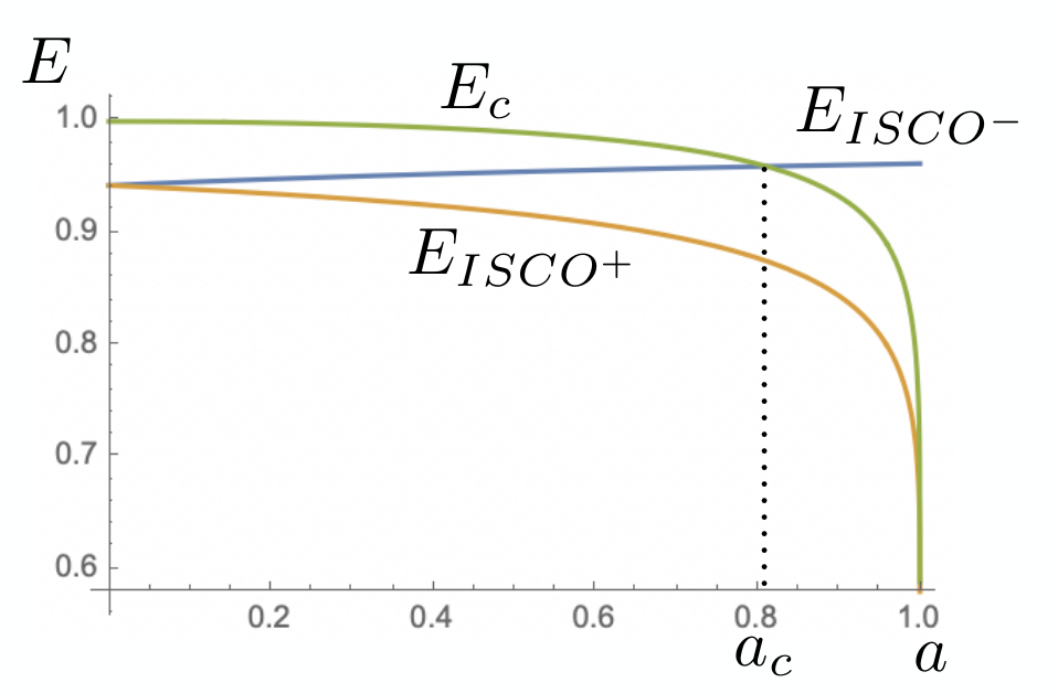
This function of aa is plotted on Figure 1. It obeys E+<EcE_{+}<E_{c} for all 0≤a≤10\leq a\leq 1.

We, therefore, obtain that for ℓ=ℓ+​(E)\ell=\ell_{+}(E), Q=Qs​(E)Q=Q^{\text{s}}(E) with Ec≤E<1E_{c}\leq E<1, spherical orbits exist in the phase space with root structure |∙−∙∙−⟩{|\hskip-7.0pt\bullet-\bullet\hskip-6.0pt\bullet\hskip 2.0pt-\rangle}. For ℓ=ℓ+​(E)\ell=\ell_{+}(E), Q≲Qs​(E)Q\lesssim Q^{\text{s}}(E), the root structure becomes |∙−∙+∙−⟩{|\hskip-7.0pt\bullet-\bullet+\bullet\hskip 2.0pt-\rangle}. Since there is no other double root outside the horizon and no horizon touching root, the root structure |∙−∙+∙−⟩{|\hskip-7.0pt\bullet-\bullet+\bullet\hskip 2.0pt-\rangle} is valid in the entire range 0≤Q≤Qs​(E)0\leq Q\leq Q^{\text{s}}(E). For ℓ=ℓ+​(E)\ell=\ell_{+}(E), Q≳Qs​(E)Q\gtrsim Q^{\text{s}}(E), the root structure becomes |∙−⟩{|\hskip-7.0pt\bullet-\rangle}. Again, since there are no further double roots and no horizon touching root, this root structure is valid for the entire range Q>max​{0,Qs​(E)}Q>\text{max}\{0,Q^{\text{s}}(E)\}. For ℓ=ℓ+​(E)\ell=\ell_{+}(E) and E≥1E\geq 1 and any Q≥0Q\geq 0 there is a single root structure since the roots never cross in the exterior region r+≤r<∞r_{+}\leq r<\infty and never become double. After explicit evaluation for a particular case we find the root structure |∙−∙+⟩{|\hskip-7.0pt\bullet-\bullet+\rangle}.

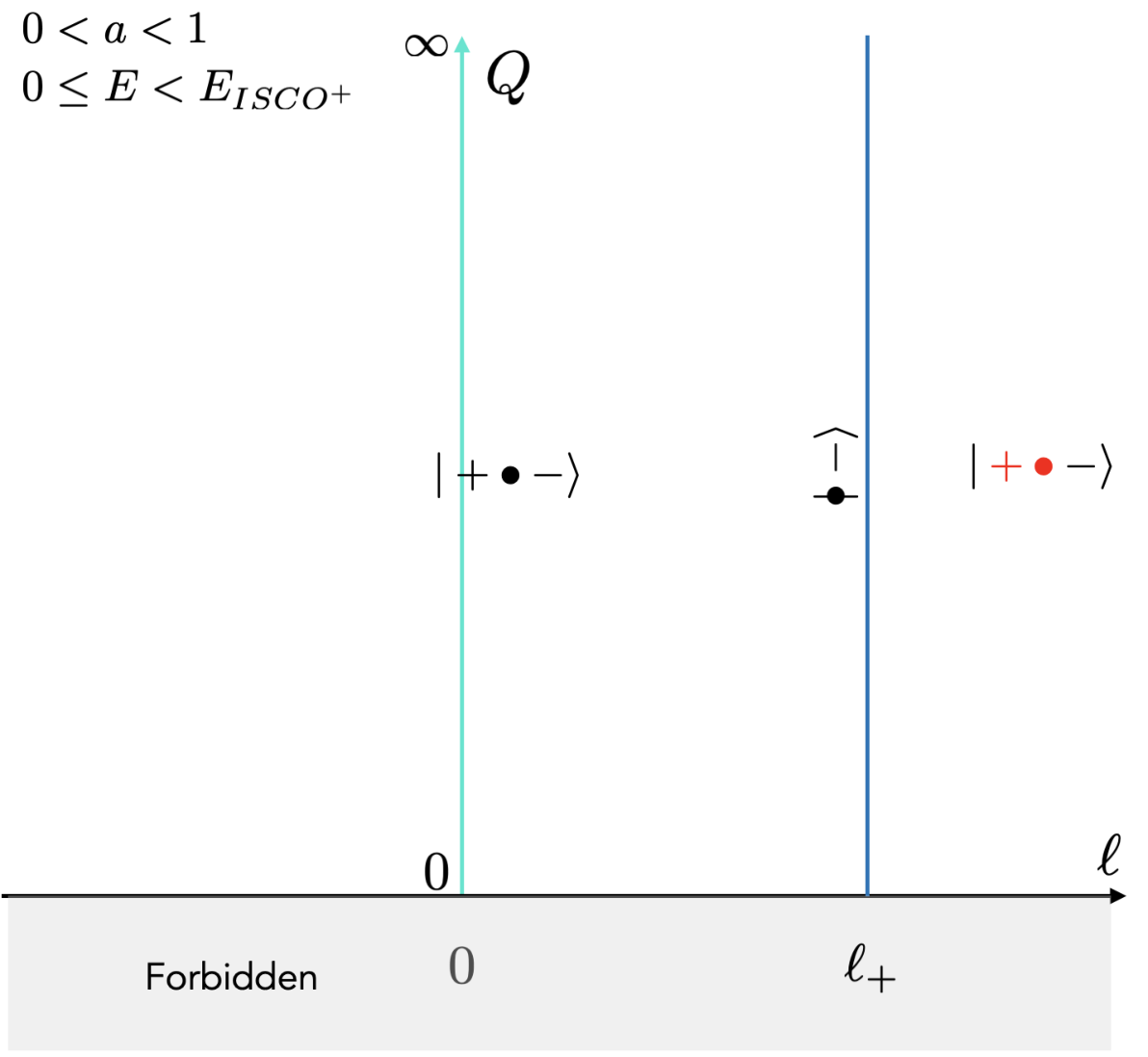
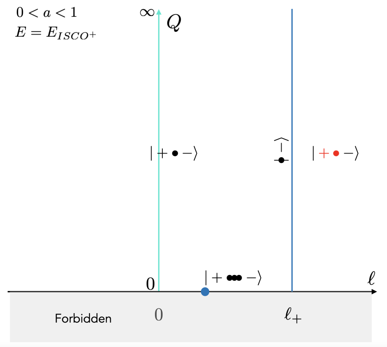
For ℓ​​ℓ+​(E)\ell\,\includegraphics[scale]{simneq.pdf}\,\ell_{+}(E) [ℓ\ell close to but not equal to ℓ+​(E)\ell_{+}(E)], the root at the horizon moves towards positive radius, which allows orbits close to the horizon. The phase space of root structures that admit at least one root at or close to the horizon is summarized on Figure 2.

We finally note that there is a special value

ac≈0.8109337526a_{c}\approx 0.8109337526 (3.16)

of aa such that the energy EcE_{c} coincides with the energy EI​S​C​O−E_{ISCO^{-}} at the retrograde ISCO as defined in (3.28) in section 3.3. For that special value of aa and the corresponding special energy E=Ec=EI​S​C​O−≈0.9598057008E=E_{c}=E_{ISCO^{-}}\approx 0.9598057008, both orbit classes |∙−∙∙−⟩{|\hskip-7.0pt\bullet-\bullet\hskip-6.0pt\bullet\hskip 2.0pt-\rangle} and |+∙∙∙−⟩|+\bullet\hskip-5.0pt\bullet\hskip-5.0pt\bullet\hskip 2.0pt-\rangle are equatorial (Q=0Q=0) orbit classes (with a distinct angular momentum).

EcE_{c} EI​S​C​O+E_{{ISCO}^{+}} EI​S​C​O−E_{{ISCO}^{-}}
a=0a=0 11 2​23\frac{2\sqrt{2}}{3} 2​23\frac{2\sqrt{2}}{3}
a=1a=1 13\frac{1}{\sqrt{3}} 13\frac{1}{\sqrt{3}} 53​3\frac{5}{3\sqrt{3}}
Table 4: Energy EcE_{c} and EI​S​C​O±E_{{ISCO}^{\pm}} in the Schwarzschild and extreme Kerr limit.

In the Schwarzschild and extreme Kerr limit, the energy EI​S​C​O±E_{{ISCO}^{\pm}} and EcE_{c} are shown in Table 4. When a=0a=0, the two ISCO branches merge as they should for the Schwarzschild black hole.
Refer to caption
Figure 1: Energy EcE_{c} (corresponding to the existence of a horizon touching root and a stable double root on the equatorial plane), prograde ISCO energy EI​S​C​O+E_{ISCO^{+}} and retrograde ISCO energy EI​S​C​O−E_{ISCO^{-}} as a function of aa. The critical rotation aca_{c} is defined at the intersection between EI​S​C​O−E_{ISCO^{-}} and EcE_{c}.
Refer to caption
Figure 2: Phase space of root structures that admit at least one root at or close to the horizon and that obey the positivity bounds.

3.3 Spherical orbits

The timelike spherical orbits of Kerr, defined from R⁡(r)=R′​(r)=0R(r)=R^{\prime}(r)=0, were elegantly summarized by Teo [67] based on earlier results [70, 71, 72, 73, 74, 58]. There are 4 classes of solutions (Ei,ℓi)(E_{i},\ell_{i}), i=a′,b′,c′,d′i=\text{a}^{\prime},\text{b}^{\prime},\text{c}^{\prime},\text{d}^{\prime}. The first two are given by

Ea′,b′​(Q,r)\displaystyle E_{\text{a}^{\prime},\text{b}^{\prime}}(Q,r) =\displaystyle= r3​(r−2)−a⁡(a​Q∓Υ⁡(Q,r))r2​r3​(r−3)−2​a​(a​Q∓Υ⁡(Q,r)),\displaystyle\frac{r^{3}(r-2)-a(aQ\mp\sqrt{\Upsilon(Q,r)})}{r^{2}\sqrt{r^{3}(r-3)-2a(aQ\mp\sqrt{\Upsilon(Q,r)})}}, (3.17)
ℓa′,b′​(Q,r)\displaystyle\ell_{\text{a}^{\prime},\text{b}^{\prime}}(Q,r) =\displaystyle= −2​a​r3+(r2+a2)​(a​Q∓Υ⁡(Q,r))r2​r3​(r−3)−2​a​(a​Q∓Υ⁡(Q,r)),\displaystyle-\frac{2ar^{3}+(r^{2}+a^{2})(aQ\mp\sqrt{\Upsilon(Q,r)})}{r^{2}\sqrt{r^{3}(r-3)-2a(aQ\mp\sqrt{\Upsilon(Q,r)})}}, (3.18)

where

Υ⁡(Q,r)=r5−Q​r3​(r−3)+a2​Q2.\displaystyle\Upsilon(Q,r)=r^{5}-Qr^{3}(r-3)+a^{2}Q^{2}. (3.19)

The third and fourth are given by (Ec′,d′,ℓc′,d′)=−(Ea′,b′,ℓa′,b′)(E_{\text{c}^{\prime},\text{d}^{\prime}},\ell_{\text{c}^{\prime},\text{d}^{\prime}})=-(E_{\text{a}^{\prime},\text{b}^{\prime}},\ell_{\text{a}^{\prime},\text{b}^{\prime}}). The first and second classes continuously join. They have positive energy in the range of parameters where they exist. The range of existence is dictated by the radii of the prograde and retrograde photon orbits, respectively r1r_{1} and r2r_{2},

r1,2≡2​[1+cos⁡(23​arccos⁡(∓a))].\displaystyle r_{1,2}\equiv 2\left[1+\cos\left(\frac{2}{3}\arccos\left(\mp a\right)\right)\right]. (3.20)

They lie in the range 1≤r1<3<r2≤41\leq r_{1}<3<r_{2}\leq 4 and are the two largest roots of Ξ≡r3−6​r2+9​r−4​a2\Xi\equiv r^{3}-6r^{2}+9r-4a^{2}. The range of existence is also determined by

Q1​(r)=r22​a2​(r⁡(r−3)−r​Ξ).\displaystyle Q_{1}(r)=\frac{r^{2}}{2a^{2}}(r(r-3)-\sqrt{r\Xi}). (3.21)

In the nonextremal case, the solution a′\text{a}^{\prime} exists for r>r1r>r_{1}: for any 0≤Q<∞0\leq Q<\infty between r1<r<r2r_{1}<r<r_{2} but for 0≤Q<Q1​(r)0\leq Q<Q_{1}(r) for r≥r2r\geq r_{2}. The solution b′\text{b}^{\prime} exists for r>r2r>r_{2} in the range 0≤Q≤Q1​(r)0\leq Q\leq Q_{1}(r). In the extremal case a=1a=1, the Boyer-Linquist radius does not resolve the near-horizon region and does not lead to a rightful parametrization at r=1r=1, see [67] for a discussion.

Prograde and retrograde orbits

The solution a′\text{a}^{\prime} is either prograde or retrograde while the solution b′\text{b}^{\prime} is retrograde. The subset of polar orbits (ℓ=0\ell=0) within the solution a′\text{a}^{\prime} set are given by Q=Q0​(r)Q=Q_{0}(r) where

Q0​(r)≡r2​(Δ2+4​r2​(r−1))(r2+a2)​(r​Δ−(r2−a2)).\displaystyle Q_{0}(r)\equiv\frac{r^{2}(\Delta^{2}+4r^{2}(r-1))}{(r^{2}+a^{2})(r\Delta-(r^{2}-a^{2}))}. (3.22)

The angular momentum ℓ>0\ell>0 for Q<Q0​(r)Q<Q_{0}(r) while ℓ<0\ell<0 for Q>Q0​(r)Q>Q_{0}(r). In the range r≥r2r\geq r_{2} where Q1​(r)Q_{1}(r) is real, it obeys Q0​(r)≤Q1​(r)Q_{0}(r)\leq Q_{1}(r). We have Q0​(r)≥0Q_{0}(r)\geq 0 for r≥r0r\geq r_{0} where

r0≡1+2​3−a23​cos⁡(13​arccos⁡(3​(1−a2)3−a2​33−a2)).\displaystyle r_{0}\equiv 1+2\sqrt{\frac{3-a^{2}}{3}}\cos\left(\frac{1}{3}\arccos\left(\frac{3(1-a^{2})}{3-a^{2}}\sqrt{\frac{3}{3-a^{2}}}\right)\right). (3.23)
Marginally stable spherical orbits

The marginally stable spherical orbits R⁡(r)=R′​(r)=R′′​(r)=0R(r)=R^{\prime}(r)=R^{\prime\prime}(r)=0 obey Q=Qm​s​(r)Q=Q_{ms}(r), where

Qm​s​(r)≡−r5/2​[(Δ−2​r)2−4​a2]4​a2​(r3/2−r−Δ).\displaystyle Q_{ms}(r)\equiv-\frac{r^{5/2}[(\sqrt{\Delta}-2\sqrt{r})^{2}-4a^{2}]}{4a^{2}(r^{3/2}-\sqrt{r}-\sqrt{\Delta})}. (3.24)

In the range r≥r2r\geq r_{2}, where Q1​(r)Q_{1}(r) is real, Qm​s​(r)≤Q1​(r)Q_{ms}(r)\leq Q_{1}(r). The locus where Qm​s​(r)=Q1​(r)Q_{ms}(r)=Q_{1}(r) is r=rm​s∗r=r_{ms}^{*} where

rm​s∗≡[114+72​cos⁡(13​arccos⁡(143+200​a2343))].\displaystyle r_{ms}^{*}\equiv\left[\frac{11}{4}+\frac{7}{2}\cos\left(\frac{1}{3}\arccos\left(\frac{143+200a^{2}}{343}\right)\right)\right]. (3.25)

When Q=0Q=0, the prograde and retrograde marginally stable orbits are located at r=rm​s±r=r_{ms}^{\pm}, where

rm​s±\displaystyle r_{ms}^{\pm} ≡\displaystyle\equiv {3+Z2∓(3−Z1)​(3+Z1+2​Z2)},\displaystyle\left\{3+Z_{2}\mp\sqrt{(3-Z_{1})(3+Z_{1}+2Z_{2})}\right\}, (3.26)
Z1\displaystyle Z_{1} ≡\displaystyle\equiv 1+(1−a2)1/3​[(1+a)1/3+(1−a)1/3],Z2≡3​a2+(Z1)2.\displaystyle 1+(1-a^{2})^{1/3}\left[(1+a)^{1/3}+(1-a)^{1/3}\right],\qquad Z_{2}\equiv\sqrt{3a^{2}+(Z_{1})^{2}}.

The class a′\text{a}^{\prime} of marginally stable orbits lie in the range rm​s+≤r≤rm​s∗r_{ms}^{+}\leq r\leq r_{ms}^{*}. Stability occurs for 0≤Q<Qm​s​(r)0\leq Q<Q_{ms}(r), and unstability for Qm​s​(r)<Q<∞Q_{ms}(r)<Q<\infty. The class b′\text{b}^{\prime} of marginally stable orbits smoothly joins in the next range rm​s∗≤r≤rm​s−r_{ms}^{*}\leq r\leq r_{ms}^{-}. Unstability occurs for 0≤Q<Qm​s​(r)0\leq Q<Q_{ms}(r) and stability for Qm​s​(r)<Q≤Q1​(r)Q_{ms}(r)<Q\leq Q_{1}(r). The energy of the prograde and retrograde ISCO (Q=0Q=0) orbits are respectively given by

EI​S​C​O+\displaystyle E_{ISCO^{+}} =\displaystyle= Ea′​(0,rm​s+),\displaystyle E_{\text{a}^{\prime}}(0,r^{+}_{ms}), (3.27)
EI​S​C​O−\displaystyle E_{ISCO^{-}} =\displaystyle= Eb′​(0,rm​s−).\displaystyle E_{\text{b}^{\prime}}(0,r^{-}_{ms}). (3.28)
Marginally bound spherical orbits

The marginally bound spherical orbits R⁡(r)=R′​(r)=0R(r)=R^{\prime}(r)=0 and E2=1E^{2}=1 obey Q=Qm​b​(r)Q=Q_{mb}(r) where

Qm​b​(r)≡−r2​[r​(r−2)2−a2]a2​(r−1)2.\displaystyle Q_{mb}(r)\equiv-\frac{r^{2}[r(\sqrt{r}-2)^{2}-a^{2}]}{a^{2}(\sqrt{r}-1)^{2}}. (3.29)

When Q=0Q=0, the prograde and retrograde marginally bound circular orbits lie at r=rm​b+≡(1+1−a)2r=r_{mb}^{+}\equiv(1+\sqrt{1-a})^{2} and r=rm​b−≡(1+1+a)2r=r_{mb}^{-}\equiv(1+\sqrt{1+a})^{2}.

In the range r≥r2r\geq r_{2}, where Q1​(r)Q_{1}(r) is real, Qm​b​(r)≤Q1​(r)Q_{mb}(r)\leq Q_{1}(r). Equality Qm​b​(r)=Q1​(r)Q_{mb}(r)=Q_{1}(r) occurs at r=rm​b∗r=r_{mb}^{*}, where rm​b∗r_{mb}^{*} is the largest real root of the quintic r2​Ξ−Δ2=0r^{2}\Xi-\Delta^{2}=0. Note that the largest root flips only at a=155/2​2​1293/2−383a=\frac{1}{5^{5/2}\sqrt{2}}\sqrt{129^{3/2}-383}. It obeys rm​b+≤rm​b∗≤rm​b−r_{mb}^{+}\leq r_{mb}^{*}\leq r_{mb}^{-}.

The class a′\text{a}^{\prime} of marginally bound orbits lie in the range rm​b+≤r≤rm​b∗r_{mb}^{+}\leq r\leq r_{mb}^{*}. Bound orbits have 0≤Q<Qm​b​(r)0\leq Q<Q_{mb}(r), and unbound spherical orbits have Qm​b​(r)<Q<∞Q_{mb}(r)<Q<\infty. The class b′\text{b}^{\prime} of marginally bound orbits lie in the range rm​b∗≤r≤rm​b−r_{mb}^{*}\leq r\leq r_{mb}^{-}. Unbound spherical orbits occur for 0≤Q<Qm​b​(r)0\leq Q<Q_{mb}(r), and bound spherical orbits occur for Qm​b​(r)<Q≤Q1​(r)Q_{mb}(r)<Q\leq Q_{1}(r).

3.4 Marginal orbits

Marginal orbits are by definition orbits such that E=1E=1. The radial potential is

R⁡(r)=2​(r3−12​(Q+ℓ2)​r2+(Q+(ℓ−a)2)​r−a2​Q2).R(r)=2(r^{3}-\frac{1}{2}(Q+\ell^{2})r^{2}+(Q+(\ell-a)^{2})r-\frac{a^{2}Q}{2}). (3.30)

The horizon is located at r+=1+1−a2r_{+}=1+\sqrt{1-a^{2}}. Since R⁡(∞)>0R(\infty)>0, the root structure always takes the form |⋯+⟩|\dots+\rangle. The potential has the cubic discriminant Δ3=−108​(qr24+pr327)\Delta_{3}=-108(\frac{q_{r}^{2}}{4}+\frac{p^{3}_{r}}{27}), where

pr\displaystyle p_{r} =\displaystyle= Q+(ℓ−a)2−112​(Q+ℓ2)2,\displaystyle Q+(\ell-a)^{2}-\frac{1}{12}(Q+\ell^{2})^{2}, (3.31)
qr\displaystyle q_{r} =\displaystyle= −1108​(Q+ℓ2)3+16​(Q+ℓ2)​(Q+(ℓ−a)2)−12​Q​a2.\displaystyle-\frac{1}{108}(Q+\ell^{2})^{3}+\frac{1}{6}(Q+\ell^{2})(Q+(\ell-a)^{2})-\frac{1}{2}Qa^{2}. (3.32)

3.4.1 Double root structure

Double roots r∗r_{*} (where R⁡(r∗)=R′​(r∗)=0R(r_{*})=R^{\prime}(r_{*})=0 or Δ3=0\Delta_{3}=0) occur for two solution branches denoted as a,b\text{a},\text{b} (a is associated with the upper sign):

Q=Qa,b​(r∗)\displaystyle Q=Q_{\text{a},\text{b}}(r_{*}) ≡\displaystyle\equiv r∗2​(a2−(r∗±2)2​r∗)a2​(r∗±1)2,\displaystyle\frac{r_{*}^{2}(a^{2}-(\sqrt{r_{*}}\pm 2)^{2}r_{*})}{a^{2}(\sqrt{r_{*}}\pm 1)^{2}}, (3.33)
ℓ=ℓa,b​(r∗)\displaystyle\ell=\ell_{\text{a},\text{b}}(r_{*}) ≡\displaystyle\equiv a2±2​r∗3/2+r∗2a⁡(1±r∗).\displaystyle\frac{a^{2}\pm 2r_{*}^{3/2}+r_{*}^{2}}{a(1\pm\sqrt{r_{*}})}. (3.34)

These branches exist for the range r+≤r∗<∞r_{+}\leq r_{*}<\infty. The branches intersect in the exterior region only at the horizon where ℓa,b​(r+)=2​r+a\ell_{\text{a},\text{b}}(r_{+})=\frac{2r_{+}}{a}, Qa,b​(r+)=2​(2+r+−4​r+a2)<0Q_{\text{a},\text{b}}(r_{+})=2(2+r_{+}-\frac{4r_{+}}{a^{2}})<0. Outside the horizon we have Qa​(r∗)<Qb​(r∗)Q_{\text{a}}(r_{*})<Q_{\text{b}}(r_{*}). In terms of the double root r∗r_{*}, the third real root is a2−(r∗±2)2​r∗2​(r∗±1)2\frac{a^{2}-(\sqrt{r_{*}}\pm 2)^{2}r_{*}}{2(\sqrt{r_{*}}\pm 1)^{2}} for each solution branch. In both cases, this root is below r+r_{+} and therefore irrelevant to the motion. The root structure is therefore given for both these branches as |+∙∙+⟩|+\bullet\hskip-4.0pt\bullet\hskip 2.0pt+\rangle for r∗>r+r_{*}>r_{+} and |∙∙+⟩{\hskip 3.0pt|\hskip-9.0pt\bullet\hskip-5.0pt\bullet\hskip 2.0pt}+\rangle for r∗=r+r_{*}=r_{+}.

Orbits of either branch belong to the phase space only if the bound Qa,b≥0Q_{\text{a},\text{b}}\geq 0 is obeyed. We have ℓ+​(r∗)>0\ell_{+}(r_{*})>0. Now Qa​(r∗)≥0Q_{\text{a}}(r_{*})\geq 0 only in the range 0≤r∗≤2+a−2​1+a0\leq r_{*}\leq 2+a-2\sqrt{1+a}, which lies below the horizon. Such solution is then disallowed in the exterior region. With a notation that will match the one of Section 3.5 we define

rc(1)≡2+a+2​1+a,rc(2)≡2−a+2​1−a\begin{split}r_{c}^{(1)}&\equiv 2+a+2\sqrt{1+a},\\ r_{c}^{(2)}&\equiv 2-a+2\sqrt{1-a}\end{split} (3.35)

with r+<rc(2)<4<rc(1)r_{+}<r_{c}^{(2)}<4<r_{c}^{(1)} for 0<a<10<a<1. For the branch b, Qb​(r∗)≥0Q_{\text{b}}(r_{*})\geq 0 with r∗>r+r_{*}>r_{+} is satisfied for rc(2)≤r∗≤rc(1)r_{c}^{(2)}\leq r_{*}\leq r_{c}^{(1)}. The root structure |∙∙+⟩{\hskip 3.0pt|\hskip-9.0pt\bullet\hskip-5.0pt\bullet\hskip 2.0pt}+\rangle is therefore disallowed. We have Qb​(rc(1,2))=0Q_{\text{b}}(r_{c}^{(1,2)})=0. One can check that ℓb​(r∗)\ell_{\text{b}}(r_{*}) is a monotonically decreasing function in the range rc(2)≤r∗≤rc(1)r_{c}^{(2)}\leq r_{*}\leq r_{c}^{(1)}. It admits an inverse r∗​(ℓ)r_{*}(\ell). At the endpoints Qb​(rc(2))=Qb​(rc(1))=0Q_{\text{b}}(r_{c}^{(2)})=Q_{\text{b}}(r_{c}^{(1)})=0 and we have ℓb​(rc(2))=2​(1+1−a)\ell_{\text{b}}(r_{c}^{(2)})=2(1+\sqrt{1-a}), ℓb​(rc(1))=−2​(1+1+a)\ell_{\text{b}}(r_{c}^{(1)})=-2(1+\sqrt{1+a}). The maximum occurs at r∗=4r_{*}=4 where Qb​(4)=16Q_{\text{b}}(4)=16 and ℓb​(4)=−a\ell_{\text{b}}(4)=-a.

Since R′′​(r∗)>0R^{\prime\prime}(r_{*})>0, spherical orbits are unstable. We define the function Qu​(ℓ)≡Qb​(r∗​(ℓ))Q^{\text{u}}(\ell)\equiv Q_{\text{b}}(r_{*}(\ell)). For Q=Qu​(ℓ)Q=Q^{\text{u}}(\ell), the root structure is |+∙∙+⟩|+\bullet\hskip-4.0pt\bullet\hskip 2.0pt+\rangle. The root structure for distinct values of QQ is given on Figure 3.

Figure 3: Root structures of marginal orbits E=1E=1.

3.4.2 General root structure

Since Δ3=−4​a6\Delta_{3}=-4a^{6} for ℓ=Q=0\ell=Q=0, the double root becomes complex for Q<Qu​(ℓ)Q<Q^{\text{u}}(\ell) (i.e., the root structure is |+⟩|+\rangle) while there are three distinct real roots for Q>Qu​(ℓ)Q>Q^{\text{u}}(\ell) (i.e., the root structure is |+∙−∙+⟩|+\bullet-\bullet\hskip 2.0pt+\rangle which can be read from large QQ expansion).

The root structure changes when one root touches the horizon, which occurs at ℓ=2​r+a\ell=\frac{2r_{+}}{a} as derived in Section 3.2. We have ℓb​(rc(1))<2​r+a\ell_{\text{b}}(r_{c}^{(1)})<\frac{2r_{+}}{a}. Therefore, the curve Q=Qu​(ℓ)Q=Q^{\text{u}}(\ell) does not intersect the line ℓ=2​r+a\ell=\frac{2r_{+}}{a}. For ℓ>2​r+a\ell>\frac{2r_{+}}{a}, one also has the root structure |+∙−∙+⟩|+\bullet-\bullet\hskip 2.0pt+\rangle. Now, trapped orbits are disallowed for positive energy orbits with ℓ>ℓ+​(E)\ell>\ell_{+}(E), see Section 2.2. The root structure is therefore |+∙−∙+⟩|\hskip 2.0pt{\color[rgb]{1,0,0}+\hskip 2.0pt\bullet}-\bullet\hskip 2.0pt+\rangle. The large ℓ\ell and large QQ limit are in agreement with the analysis of Section 3.1. We conclude that the phase space is complete for E=1E=1. The classification is depicted in Figure 3.

3.5 Generic nonmarginal orbits

The radial potential (2.1) is quartic in rr for E≠1E\neq 1. The root structure for E>1E>1 takes the form |⋯+⟩|\dots+\rangle, while for E<1E<1 it takes the form |⋯−⟩|\dots-\rangle. For ℓ=ℓ+​(E)\ell=\ell_{+}(E) it takes the form |∙−⋯⟩{|\hskip-5.0pt\bullet}-\cdots\rangle, while for ℓ≠ℓ+​(E)\ell\neq\ell_{+}(E) it takes the form |+⋯⟩|+\cdots\rangle. The discriminant takes the form

Δ4=16​(1−a2)(E2−1)5​Q5+b4​(ℓ,E)​Q4+b3​(ℓ,E)​Q3+b2​(ℓ,E)​Q2+b1​(ℓ,E)​Q+b0​(ℓ,E).\Delta_{4}=\frac{16(1-a^{2})}{(E^{2}-1)^{5}}Q^{5}+b_{4}(\ell,E)Q^{4}+b_{3}(\ell,E)Q^{3}+b_{2}(\ell,E)Q^{2}+b_{1}(\ell,E)Q+b_{0}(\ell,E). (3.36)

It is a quintic function of QQ for a nonextremal black hole.

3.5.1 Double root structure

The general solution of double roots at r=r∗r=r_{*} has been solved in [67] by expressing EE and ℓ\ell as a function of r∗r_{*} and QQ as we review in Section 3.3. However, the analysis of the positivity bound on QQ is not straightforward for E>1E>1. Here, we will solve for the double roots by expressing QQ and ℓ\ell as a function of r∗r_{*} and EE.

Branches a and b.

The two branches of the solution are (aa is the upper sign)

Q=Qa,b​(E,r∗)\displaystyle Q=Q_{\text{a},\text{b}}(E,r_{*}) ≡\displaystyle\equiv r∗2a2​(r∗−1)2​(−r∗3+3​r∗2+(a2−4)​r∗+a2CLOSE\displaystyle\frac{r_{*}^{2}}{a^{2}(r_{*}-1)^{2}}(-r_{*}^{3}+3r_{*}^{2}+(a^{2}-4)r_{*}+a^{2} (3.37)
OPEN+r∗​(1−E2)​(r∗3−4​r∗2+5​r∗−2​a2)∓2​E​Δ​(r∗)​r∗​(1+(E2−1)​r∗)),\displaystyle\hskip-28.45274pt+r_{*}(1-E^{2})(r_{*}^{3}-4r_{*}^{2}+5r_{*}-2a^{2})\mp 2E\Delta(r_{*})\sqrt{r_{*}(1+(E^{2}-1)r_{*})}),
ℓ=ℓa,b​(E,r∗)\displaystyle\ell=\ell_{\text{a},\text{b}}(E,r_{*}) ≡\displaystyle\equiv E⁡(r∗2−a2)±Δ⁡(r∗)​r∗​((E2−1)​r∗+1)a⁡(r∗−1),\displaystyle\frac{E(r_{*}^{2}-a^{2})\pm\Delta(r_{*})\sqrt{r_{*}\left(\left(E^{2}-1\right)r_{*}+1\right)}}{a(r_{*}-1)}, (3.38)

where Δ⁡(r)=r2−2​r+a2\Delta(r)=r^{2}-2r+a^{2}. These solutions formally match with (3.33)–(3.34) for E=1E=1. The solution is not valid for r∗=1r_{*}=1, which coincides with the NHEK region at extremality. Since we are discussing a<1a<1, the solutions are always real in the exterior region as long as E≥Ea×b​(r∗)E\geq E_{\text{a}\times\text{b}}(r_{*}), where Ea×b​(r∗)≡1−r∗−1E_{\text{a}\times\text{b}}(r_{*})\equiv\sqrt{1-r_{*}^{-1}} is the energy at which the two branches meet. We have E+≤Ea×b​(r∗)≤1E_{+}\leq E_{\text{a}\times\text{b}}(r_{*})\leq 1, where E+E_{+} was defined in (3.11). Alternatively, the two branches a,b\text{a},\text{b} meet at r∗=ra×b​(E)≡(1−E2)−1r_{*}=r_{\text{a}\times\text{b}}(E)\equiv(1-E^{2})^{-1}. For E≥1E\geq 1, the solutions a,b\text{a},\text{b} both exist for r+≤r∗<∞r_{+}\leq r_{*}<\infty. For E+≤E<1E_{+}\leq E<1, both solutions exist in the range r+≤r∗≤ra×b​(E)r_{+}\leq r_{*}\leq r_{\text{a}\times\text{b}}(E). For E<1E<1, Qa,b​(E,ra×b​(E))<0Q_{\text{a},\text{b}}(E,r_{\text{a}\times\text{b}}(E))<0, which violates the bound (2.1). Therefore, the two branches do not meet inside the phase space for E<1E<1. For E>1E>1, ra×b​(E)<0r_{\text{a}\times\text{b}}(E)<0 and, therefore, the branches meet outside the phase space as well.

Analysis of Qa,b≥0Q_{\text{a},\text{b}}\geq 0.

We have |ℓa,b|>a​E2−1|\ell_{\text{a},\text{b}}|>a\sqrt{E^{2}-1}. Therefore, the positivity bound (2.1) for both branches a,b\text{a},\text{b} is Qa,b≥0Q_{\text{a},\text{b}}\geq 0. The roots of Qa,bQ_{\text{a},\text{b}} might only occur at (upper sign corresponds to a)

Ea,b(1)​(r∗)=∓(r∗−2)​r∗−ar∗3/4​(r∗−3)​r∗−2​a,\displaystyle E^{(1)}_{\text{a},\text{b}}(r_{*})=\mp\frac{(r_{*}-2)\sqrt{r_{*}}-a}{r_{*}^{3/4}\sqrt{(r_{*}-3)\sqrt{r_{*}}-2a}}, (3.39)
Ea,b(2)​(r∗)=∓(r∗−2)​r∗+ar∗3/4​(r∗−3)​r∗+2​a.\displaystyle E^{(2)}_{\text{a},\text{b}}(r_{*})=\mp\frac{(r_{*}-2)\sqrt{r_{*}}+a}{r_{*}^{3/4}\sqrt{(r_{*}-3)\sqrt{r_{*}}+2a}}. (3.40)

We denote by r∗(1)r_{*}^{(1)} the only root of (r∗−3)​r∗+2​a(r_{*}-3)\sqrt{r_{*}}+2a above the horizon, by r∗(2)r_{*}^{(2)} the only root of (r∗−3)​r∗−2​a(r_{*}-3)\sqrt{r_{*}}-2a above the horizon. Explicitly,

r∗(1)\displaystyle r_{*}^{(1)} =\displaystyle= 2+cos⁡(2​arcsin⁡a3)−3​sin⁡(2​arcsin⁡a3),\displaystyle 2+\cos\left(\frac{2\arcsin a}{3}\right)-\sqrt{3}\sin\left(\frac{2\arcsin a}{3}\right), (3.41)
r∗(2)\displaystyle r_{*}^{(2)} =\displaystyle= 2+cos⁡(2​arcsin⁡a3)+3​sin⁡(2​arcsin⁡a3).\displaystyle 2+\cos\left(\frac{2\arcsin a}{3}\right)+\sqrt{3}\sin\left(\frac{2\arcsin a}{3}\right). (3.42)

We have r+<r∗(1)≤r∗(2)<4r_{+}<r_{*}^{(1)}\leq r_{*}^{(2)}<4 for 0≤a<10\leq a<1. Note that Ea,b(1)E^{(1)}_{\text{a},\text{b}} is a real root in the range r∗(2)<r∗<∞r_{*}^{(2)}<r_{*}<\infty, while Ea,b(2)E^{(2)}_{\text{a},\text{b}} is a real root in the range r∗(1)<r∗<∞r_{*}^{(1)}<r_{*}<\infty.

Let us now analyze the positivity of QQ in the relevant ranges of r∗r_{*}. In the range r+≤r∗≤r∗(1)r_{+}\leq r_{*}\leq r_{*}^{(1)}, there is no real root for Qa,bQ_{\text{a},\text{b}}, and Qa,bQ_{\text{a},\text{b}} is negative, Qa,b<0Q_{\text{a},\text{b}}<0. In the range r∗(1)<r∗≤r∗(2)r_{*}^{(1)}<r_{*}\leq r_{*}^{(2)}, Ea,b(1)E^{(1)}_{\text{a},\text{b}} is complex, but Ea,b(2)E^{(2)}_{\text{a},\text{b}} is real. We have Ea(2)≤0E^{(2)}_{\text{a}}\leq 0, while Eb(2)≥0E^{(2)}_{\text{b}}\geq 0. In the entire range Ea(2)<0≤EE^{(2)}_{\text{a}}<0\leq E, we have Qa<0Q_{\text{a}}<0. For branch b, Qb≥0Q_{\text{b}}\geq 0 only for E≥Eb(2)E\geq E^{(2)}_{\text{b}}. Finally, in the range r∗(2)<r∗<∞r_{*}^{(2)}<r_{*}<\infty, both roots Ea,b(1,2)E^{(1,2)}_{\text{a,b}} are real for each branch. We find Ea(1,2)<0E_{\text{a}}^{(1,2)}<0. Then, in the entire range Ea(1,2)<0≤EE_{\text{a}}^{(1,2)}<0\leq E, we find Qa<0Q_{\text{a}}<0. Instead, we have 0<Eb(2)<Eb(1)0<E_{\text{b}}^{(2)}<E_{\text{b}}^{(1)}, and we find that Qb≥0Q_{\text{b}}\geq 0 in the range Eb(2)≤E≤Eb(1)E_{\text{b}}^{(2)}\leq E\leq E_{\text{b}}^{(1)}.

We conclude that the branch a lies outside the phase space and we, therefore, discard it. In the range Eb(2)≤EE_{\text{b}}^{(2)}\leq E, branch b is allowed for r∗(1)<r∗≤r∗(2)r_{*}^{(1)}<r_{*}\leq r_{*}^{(2)}. In the range Eb(2)≤E≤Eb(1)E_{\text{b}}^{(2)}\leq E\leq E_{\text{b}}^{(1)}, branch b is allowed for r∗(2)<r∗<∞r_{*}^{(2)}<r_{*}<\infty. The final allowed range is therefore the union of the regions

r∗(1)<r∗≤r∗(2)&Eb(2)≤Er_{*}^{(1)}<r_{*}\leq r_{*}^{(2)}\quad\&\quad E_{\text{b}}^{(2)}\leq E (3.43)

and

r∗(2)<r∗<∞&Eb(2)≤E≤Eb(1).r_{*}^{(2)}<r_{*}<\infty\quad\&\quad E_{\text{b}}^{(2)}\leq E\leq E_{\text{b}}^{(1)}. (3.44)
Decomposition of the region Qb≥0Q_{\text{b}}\geq 0 for E>1E>1 and E≤1E\leq 1.

The slicing of the allowed region with fixed energy EE will be performed on Figure 5. As a preparation, let us derive the allowed region Q≥0Q\geq 0 for E>1E>1 and E≤1E\leq 1. Let us denote rc(1,2)r_{c}^{(1,2)} as the only root of Eb(1,2)−1E_{\text{b}}^{(1,2)}-1 above the horizon. We have

rc(1)\displaystyle r_{c}^{(1)} =\displaystyle= 2+a+2​1+a,\displaystyle 2+a+2\sqrt{1+a}, (3.45)
rc(2)\displaystyle r_{c}^{(2)} =\displaystyle= 2−a+2​1−a.\displaystyle 2-a+2\sqrt{1-a}. (3.46)

This definition agrees with (3.35). We have Eb(1)>1E_{b}^{(1)}>1 for r∗(2)<r∗<rc(1)r_{*}^{(2)}<r_{*}<r_{c}^{(1)}, while Eb(2)>1E_{b}^{(2)}>1 for r∗(1)<r∗<rc(2)r_{*}^{(1)}<r_{*}<r_{c}^{(2)}. The four special functions r∗(1,2)r_{*}^{(1,2)}, rc(1,2)r_{c}^{(1,2)} of aa are plotted on Figure 4. There is a single aa where there is an intersection of two such functions. We denote a^c≈0.313708\hat{a}_{c}\approx 0.313708 the critical aa such that r∗(2)=rc(2)r_{*}^{(2)}=r_{c}^{(2)}. For 0≤a<a^c0\leq a<\hat{a}_{c}, we have r∗(1)≤r∗(2)<rc(2)<rc(1)r_{*}^{(1)}\leq r_{*}^{(2)}<r_{c}^{(2)}<r_{c}^{(1)}, while for a^c≤a<1\hat{a}_{c}\leq a<1, we have r∗(1)<rc(2)≤r∗(2)<rc(1)r_{*}^{(1)}<r_{c}^{(2)}\leq r_{*}^{(2)}<r_{c}^{(1)}.

From now on, we discard branch a and drop the labels b in all quantities. Instead of (3.39)–(3.40), we now denote

E(1)​(r∗)≡(r∗−2)​r∗−ar∗3/4​(r∗−3)​r∗−2​a,\displaystyle E^{(1)}(r_{*})\equiv\frac{(r_{*}-2)\sqrt{r_{*}}-a}{r_{*}^{3/4}\sqrt{(r_{*}-3)\sqrt{r_{*}}-2a}}, (3.47)
E(2)​(r∗)≡(r∗−2)​r∗+ar∗3/4​(r∗−3)​r∗+2​a.\displaystyle E^{(2)}(r_{*})\equiv\frac{(r_{*}-2)\sqrt{r_{*}}+a}{r_{*}^{3/4}\sqrt{(r_{*}-3)\sqrt{r_{*}}+2a}}. (3.48)

Finally, for E<1E<1 the only allowed range is

rc(2)≤r∗<∞&E(2)≤E<min​(1,E(1)).r_{c}^{(2)}\leq r_{*}<\infty\;\&\;E^{(2)}\leq E<\text{min}(1,E^{(1)}). (3.49)

For E≥1E\geq 1, the range such that Q≥0Q\geq 0 is

r∗(1)<r∗≤r∗(2)&E≥max​(1,E(2)),r_{*}^{(1)}<r_{*}\leq r_{*}^{(2)}\;\&\;E\geq\text{max}(1,E^{(2)}), (3.50)

together with

r∗(2)<r∗≤rc(1)&max​(1,E(2))≤E≤E(1).r_{*}^{(2)}<r_{*}\leq r_{c}^{(1)}\;\&\;\text{max}(1,E^{(2)})\leq E\leq E^{(1)}. (3.51)

For r∗→∞r_{*}\to\infty, both E(1)E^{(1)} and E(2)E^{(2)} approach 11 from below.

Figure 4: Several critical radii of interest for the analysis of Q≥0Q\geq 0 in the presence of double roots.
Additional simple roots

After imposing (3.37)–(3.38) (for the branch b), the residual potential Y⁡(r)≡R⁡(r)/(r−r∗)2Y(r)\equiv R(r)/(r-r_{*})^{2} is quadratic in rr. Its discriminant is quartic in EE and vanishes for

E=±r∗​(r∗−2)​(r∗2+r∗−1)+a2​(r∗−1)​(2​r∗+1)+a4±2​−(1−a2)​r∗​Δ​(r∗)(r∗2+a2)2−4​r∗2,E=\pm\sqrt{\frac{r_{*}(r_{*}-2)(r_{*}^{2}+r_{*}-1)+a^{2}(r_{*}-1)(2r_{*}+1)+a^{4}\pm 2\sqrt{-(1-a^{2})r_{*}\Delta(r_{*})}}{(r_{*}^{2}+a^{2})^{2}-4r_{*}^{2}}},

which are always complex numbers for r∗>r+r_{*}>r_{+} since (1−a2)​r∗​Δ​(r∗)>0(1-a^{2})r_{*}\Delta(r_{*})>0. Since the discriminant is positive for any particular choice of parameters with r∗>r+r_{*}>r_{+}, it implies that the two residual roots are always real for r∗>r+r_{*}>r_{+}. In the large QQ limit, one of these roots is always below the horizon and the other one, which we will call rsr_{s} is always above the horizon, or at the horizon in the special case ℓ=ℓ+​(E)\ell=\ell_{+}(E). Since the horizon touching only occurs at ℓ=ℓ+​(E)\ell=\ell_{+}(E) as studied in Section 3.2 and, in particular, does not occur at specific QQ, we deduce that the root structure is general: only one additional root rsr_{s} is above the horizon for ℓ≠ℓ+​(E)\ell\neq\ell_{+}(E), and it coincides with the horizon for ℓ=ℓ+​(E)\ell=\ell_{+}(E). The separatrix between the position of the roots, rs<r∗r_{s}<r_{*} or rs>r∗r_{s}>r_{*}, is determined by the triple root rs=r∗r_{s}=r_{*}, which will be analyzed below.

Triple roots (ISSO).

Triple roots occur for

E\displaystyle E =\displaystyle= Etriple​(r∗)≡12​r∗​(4​r∗4−15​r∗3+21​r∗2−(10+3​a2)​r∗+3​a2)+(Δ⁡(r∗))3/2r∗3/2​(r∗3−3​r∗2+3​r∗−a2),\displaystyle E^{\text{triple}}(r_{*})\equiv\frac{1}{2}\sqrt{\frac{\sqrt{r_{*}}(4r_{*}^{4}-15r_{*}^{3}+21r_{*}^{2}-(10+3a^{2})r_{*}+3a^{2})+(\Delta(r_{*}))^{3/2}}{r_{*}^{3/2}(r_{*}^{3}-3r_{*}^{2}+3r_{*}-a^{2})}}, (3.52)
ℓ\displaystyle\ell =\displaystyle= ℓtriple​(r∗)≡Etriple​(r∗)×a4+6​a2​r∗2+2​(r∗​Δ​(r∗))3/2−6​a2​r∗−3​r∗4+2​r∗3a3+a​r∗​(−4​r∗2+9​r∗−6),\displaystyle\ell^{\text{triple}}(r_{*})\equiv E^{\text{triple}}(r_{*})\times\frac{a^{4}+6a^{2}r_{*}^{2}+2\left(r_{*}\Delta(r_{*})\right)^{3/2}-6a^{2}r_{*}-3r_{*}^{4}+2r_{*}^{3}}{a^{3}+ar_{*}\left(-4r_{*}^{2}+9r_{*}-6\right)}, (3.53)
Q\displaystyle Q =\displaystyle= Qtriple​(r∗)≡−3​a2​r∗4−a2​r∗3−3​r∗5/2​(Δ⁡(r∗))3/2+r∗6−3​r∗5+6​r∗44​a2​(a2−r∗​((r∗−3)​r∗+3)).\displaystyle Q^{\text{triple}}(r_{*})\equiv\frac{-3a^{2}r_{*}^{4}-a^{2}r_{*}^{3}-3r_{*}^{5/2}\left(\Delta(r_{*})\right)^{3/2}+r_{*}^{6}-3r_{*}^{5}+6r_{*}^{4}}{4a^{2}\left(a^{2}-r_{*}((r_{*}-3)r_{*}+3)\right)}. (3.54)

There are no quadrupole roots. The argument of the square root is positive in the exterior region r∗≥r+r_{*}\geq r_{+}. The function EtripleE^{\text{triple}} is monotonically increasing along r∗r_{*} and asymptotes to 1 as r∗→∞r_{*}\rightarrow\infty. For E<1E<1, the positivity bound is Q≥0Q\geq 0. The triple root is physically associated with the ISSO. It belongs to the allowed range (3.49) as long as E(2)≤Etriple≤E(1)E^{(2)}\leq E^{\text{triple}}\leq E^{(1)}, which amounts to rmin≤r∗≤rmaxr^{\text{min}}\leq r_{*}\leq r^{\text{max}} where rminr^{\text{min}} is the only radius above r+r_{+} such that Etriple=E(2)E^{\text{triple}}=E^{(2)}, and rmaxr^{\text{max}} is the only radius above r+r_{+} such that Etriple=E(1)E^{\text{triple}}=E^{(1)}. We have rc(2)<rmin≤rmaxr_{c}^{(2)}<r^{\text{min}}\leq r^{\text{max}}. Since Q=0Q=0 and ℓ>0\ell>0 at E=E(2)​(rmin)E=E^{(2)}(r^{\text{min}}), the critical radius rminr^{\text{min}} is nothing else than the prograde ISCO radius rI​S​C​O+≡rminr_{ISCO^{+}}\equiv r^{\text{min}}. Since Q=0Q=0 and ℓ<0\ell<0 at E=E(1)​(rmax)E=E^{(1)}(r^{\text{max}}), the critical radius rmaxr^{\text{max}} is nothing else than the retrograde ISCO radius rI​S​C​O−≡rmaxr_{ISCO^{-}}\equiv r^{\text{max}}. We denote EI​S​C​O+≡E(2)​(rI​S​C​O+)E_{ISCO^{+}}\equiv E^{(2)}(r_{ISCO^{+}}), EI​S​C​O−=E(1)​(rI​S​C​O−)E_{ISCO^{-}}=E^{(1)}(r_{ISCO^{-}}). The standard expressions for rI​S​C​O±r_{ISCO^{\pm}} are recalled in Section 3.3.

In the range rc(2)≤r∗<∞r_{c}^{(2)}\leq r_{*}<\infty, the function Etriple​(r∗)E^{\text{triple}}(r_{*}) is monotonically increasing. We denote its inverse as rI​S​S​O​(E)≡r∗triple​(E)r_{ISSO}(E)\equiv r_{*}^{\text{triple}}(E). In the allowed range rI​S​C​O+<rI​S​S​O​(E)<rI​S​C​O−r_{ISCO^{+}}<r_{ISSO}(E)<r_{ISCO^{-}} the root system is finally |+∙∙∙−⟩{|+\bullet\hskip-5.0pt\bullet\hskip-5.0pt\bullet}\hskip 2.0pt-\rangle. It describes the ISSO as well as plunging orbits.

Double roots with ℓ=0\ell=0

Branch b has ℓb​(r∗)=0\ell_{\text{b}}(r_{*})=0 for

E=E(0)​(r∗)≡Δ⁡(r∗)​r∗r∗2+a2​r∗3−3​r∗2+a2​r∗+a2.\displaystyle E=E^{(0)}(r_{*})\equiv\frac{\Delta(r_{*})\sqrt{r_{*}}}{\sqrt{r_{*}^{2}+a^{2}}\sqrt{r_{*}^{3}-3r_{*}^{2}+a^{2}r_{*}+a^{2}}}. (3.55)

Here r∗(0)<r∗r_{*}^{(0)}<r_{*} where r∗(0)r_{*}^{(0)} is the real root of r∗3−3​r∗2+a2​r∗+a2r_{*}^{3}-3r_{*}^{2}+a^{2}r_{*}+a^{2} above the horizon. The function r∗(0)r_{*}^{(0)} of aa is monotonically decreasing from r∗(0)=3r_{*}^{(0)}=3 for a=0a=0 to r∗(0)=1+2r_{*}^{(0)}=1+\sqrt{2} for a=1a=1. The condition 1+(E2−1)​r∗≥01+(E^{2}-1)r_{*}\geq 0 is precisely r∗(0)≤r∗r_{*}^{(0)}\leq r_{*}. The phase space therefore contains the branch ℓ=0\ell=0, E=E(0)​(r∗)E=E^{(0)}(r_{*}), Q=Qb​(E(0)​(r∗),r∗)≡Q∗(0)​(r∗)Q=Q_{\text{b}}(E^{(0)}(r_{*}),r_{*})\equiv Q_{*}^{(0)}(r_{*}) for r∗(0)<r∗<∞r_{*}^{(0)}<r_{*}<\infty where

Q∗(0)​(r∗)=r∗2​(r∗4+2​a2​r∗​(r∗−2)+a4)(r∗2+a2)​(r∗3−3​r∗2+a2​r∗+a2).Q_{*}^{(0)}(r_{*})=\frac{r_{*}^{2}(r_{*}^{4}+2a^{2}r_{*}(r_{*}-2)+a^{4})}{(r_{*}^{2}+a^{2})(r_{*}^{3}-3r_{*}^{2}+a^{2}r_{*}+a^{2})}. (3.56)

There is a radius r∗=rc(0)r_{*}=r_{c}^{(0)} such that Etriple​(r∗)=E(0)​(r∗)E^{\text{triple}}(r_{*})=E^{(0)}(r_{*}). The value of rc(0)r_{c}^{(0)} could be found by searching the solution ℓtriple​(r∗)=0\ell^{\text{triple}}(r_{*})=0 between rISCO+r_{\text{ISCO+}} and rISCO-r_{\text{ISCO-}}. It turns out that rc(0)r_{c}^{(0)} is the unique real solution of the equation

r6−6​r5+3​a2​r4+4​a2​r3+3​a4​r2−6​a4​r+a6=0,r^{6}-6r^{5}+3a^{2}r^{4}+4a^{2}r^{3}+3a^{4}r^{2}-6a^{4}r+a^{6}=0, (3.57)

which is larger than r+r_{+}. It is monotonically decreasing from rc(0)​(a=0)=6r_{c}^{(0)}(a=0)=6 to rc(0)​(a=1)=1+3+3+2​3r_{c}^{(0)}(a=1)=1+\sqrt{3}+\sqrt{3+2\sqrt{3}}.

Refer to caption
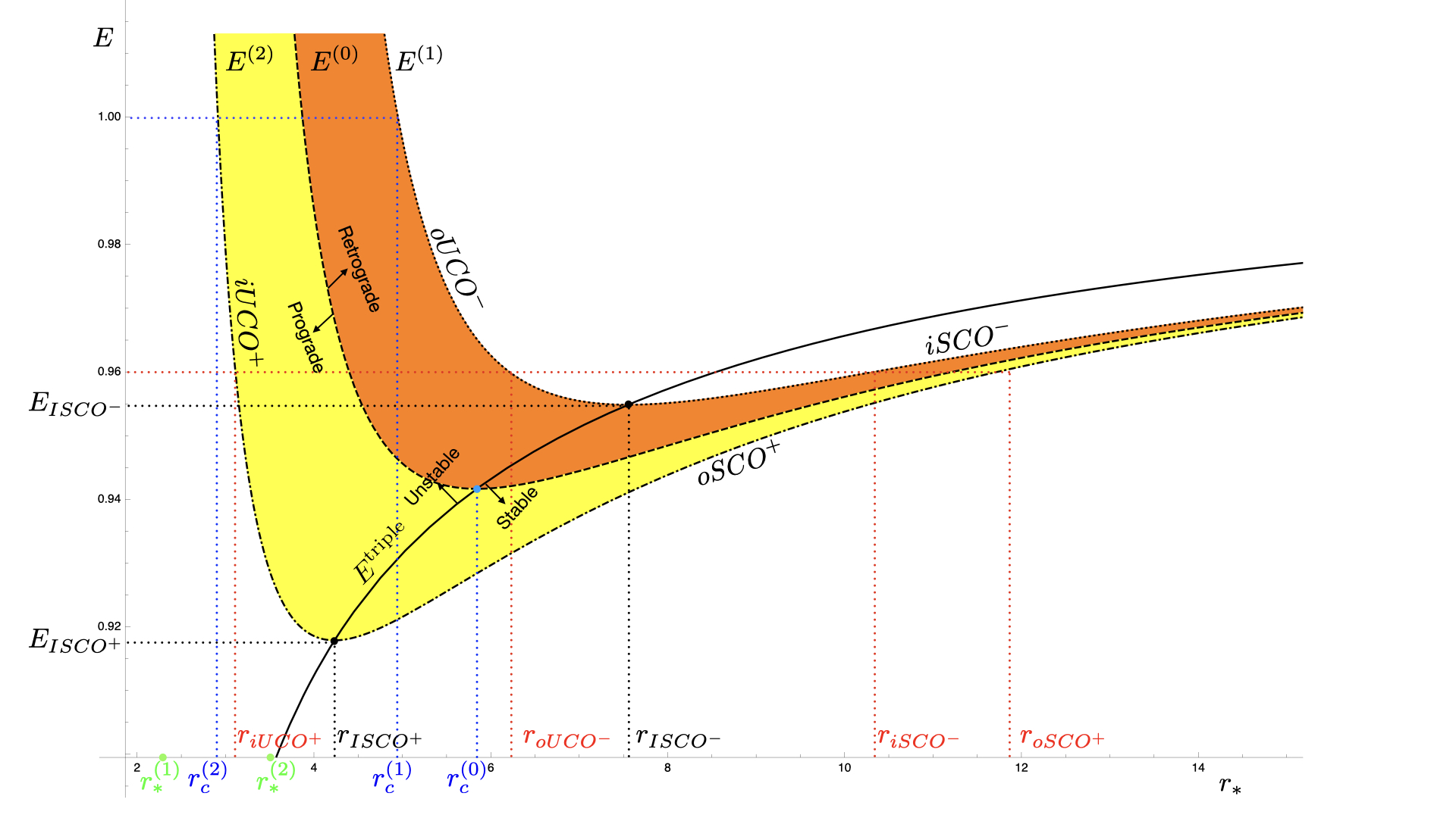
Figure 5: Functions E(0,1,2)​(r∗)E^{(0,1,2)}(r_{*}) and Etriple​(r∗)E^{\text{triple}}(r_{*}) depicted for a=1/2a=1/2 without loss of generality. The double roots are allowed both in the orange region (retrograde orbits: ℓ<0\ell<0) and the yellow region (prograde orbits: ℓ>0\ell>0). The orbits corresponding to triple roots exist (i.e., obey the positivity bound) only in the interval rI​S​C​O+≤r∗≤rI​S​C​O−r_{ISCO^{+}}\leq r_{*}\leq r_{ISCO^{-}} or EI​S​C​O+≤E≤EI​S​C​O−E_{ISCO^{+}}\leq E\leq E_{ISCO^{-}}. We also depicted the four roots ri​U​C​O+<ro​U​C​O−<ri​S​C​O−<ro​S​C​O+r_{iUCO^{+}}<r_{oUCO^{-}}<r_{iSCO^{-}}<r_{oSCO^{+}} for a specific EI​S​C​O−<E<1E_{ISCO^{-}}<E<1.
Structure of double roots

We can now deduce the root structure of the roots that contain a double root as follows. Only branch b exists in the phase space. Figure 5 shows the allowed region for the double and triple roots. When E<1E<1, the branch E(2)E^{(2)} denotes the energy of the inner unstable prograde circular orbits (i​U​C​O+iUCO^{+}), whose locations are denoted as ri​U​C​O+r_{iUCO^{+}} in the region rc(2)<ri​U​C​O+<rI​S​C​O+r_{c}^{(2)}<r_{iUCO^{+}}<r_{ISCO^{+}}, and the energy of the outer stable prograde circular orbits (o​S​C​O+oSCO^{+}) whose locations are denoted as ro​S​C​O+r_{oSCO^{+}} in the region rI​S​C​O+<ro​S​C​O+<∞r_{ISCO^{+}}<r_{oSCO^{+}}<\infty. The branch E(1)E^{(1)} denotes the energy of the inner stable retrograde circular orbits (i​S​C​O−iSCO^{-}), whose locations are denoted as ri​S​C​O−r_{iSCO^{-}} in the region rI​S​C​O−<ri​S​C​O−<∞r_{ISCO^{-}}<r_{iSCO^{-}}<\infty, and the energy of the outer unstable retrograde circular orbits (o​U​C​O−oUCO^{-}), whose locations are denoted by ro​U​C​O−r_{oUCO^{-}} in the region rc(1)<ro​U​C​O−<rI​S​C​O−r_{c}^{(1)}<r_{oUCO^{-}}<r_{ISCO^{-}}. When E≥1E\geq 1, the branch E(1)E^{(1)} denotes the energy of o​U​C​O−oUCO^{-} in the region r∗(2)<ro​U​C​O−≤rc(1)r_{*}^{(2)}<r_{oUCO^{-}}\leq r_{c}^{(1)}, while the branch E(2)E^{(2)} denotes the energy of i​U​C​O+iUCO^{+} in the region r∗(1)<ri​U​C​O+≤rc(2)r_{*}^{(1)}<r_{iUCO^{+}}\leq r_{c}^{(2)}. We discuss the structure according to the energy EE (which intersects as straight lines the allowed region of Figure 5) as follows:

  • •

    For 0<E<EI​S​C​O+0<E<E_{ISCO^{+}}, there is no double root. By continuity with the large QQ limit, the root structure is |+∙−⟩{|+\bullet\hskip 2.0pt-\rangle} for ℓ≠ℓ+​(E)\ell\neq\ell_{+}(E) and |∙−⟩{|\hskip-7.0pt\bullet-\rangle} for ℓ=ℓ+​(E)\ell=\ell_{+}(E).

  • •

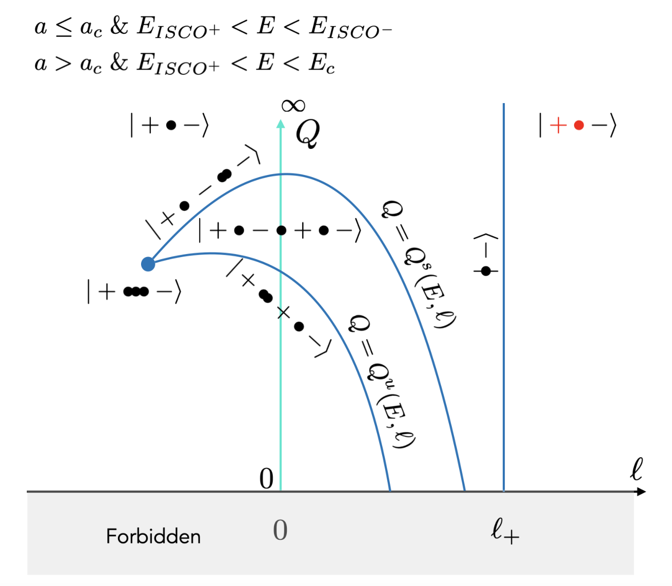
    For EI​S​C​O+≤E≤EI​S​C​O−E_{ISCO^{+}}\leq E\leq E_{ISCO^{-}}, Qb​(E,r∗)Q_{\text{b}}(E,r_{*}) is non-negative for ri​U​C​O+≤r∗≤ro​S​C​O+r_{iUCO^{+}}\leq r_{*}\leq r_{oSCO^{+}}, and it vanishes at ri​U​C​O+r_{iUCO^{+}} and ro​S​C​O+r_{oSCO^{+}}. The double root r∗r_{*} becomes a triple root if and only if r∗=rI​S​S​O​(E)r_{*}=r_{ISSO}(E) with root structure |+∙∙∙−⟩{|+\bullet\hskip-5.0pt\bullet\hskip-5.0pt\bullet}\hskip 2.0pt-\rangle.

    For r∗r_{*} in the range ri​U​C​O+≤r∗<rI​S​S​O​(E)r_{iUCO^{+}}\leq r_{*}<r_{ISSO}(E), the root structure is |+∙∙+∙−⟩{|+\bullet\hskip-3.0pt\bullet}+\bullet\hskip 2.0pt-\rangle. The double root r∗r_{*} corresponds to unstable circular orbits since R′′​(r∗)>0R^{\prime\prime}(r_{*})>0. The angular momentum is monotonously decreasing for ri​U​C​O+≤r∗≤rISSO​(E)r_{iUCO^{+}}\leq r_{*}\leq r_{\text{ISSO}}(E). In this region, one can define a unique inverse solution r^∗u​(ℓ,E)\hat{r}^{u}_{*}(\ell,E) of ℓ=ℓb​(E,r∗)\ell=\ell_{b}(E,r_{*}) at fixed EE. The function Qu​(E,ℓ)Q^{u}(E,\ell) is defined by substituting the inverse solution r^∗u​(ℓ,E)\hat{r}^{u}_{*}(\ell,E) into Qb​(E,r∗)Q_{b}(E,r_{*}),

    Qu​(E,ℓ)≡Qb​(E,r^∗u​(ℓ,E)).Q^{u}(E,\ell)\equiv Q_{b}(E,\hat{r}_{*}^{u}(\ell,E)). (3.58)

    For r∗r_{*} in the range rISSO​(E)<r∗≤ro​S​C​O+r_{\text{ISSO}}(E)<r_{*}\leq r_{oSCO^{+}} the root structure is |+∙−∙∙−⟩{|+\bullet-\bullet\hskip-3.0pt\bullet}\hskip 2.0pt-\rangle. The double root r∗r_{*} corresponds to stable circular orbits since R′′​(r∗)<0R^{\prime\prime}(r_{*})<0. The angular momentum is monotonously increasing for rISSO​(E)≤r∗≤ro​S​C​O+r_{\text{ISSO}}(E)\leq r_{*}\leq r_{oSCO^{+}}. In this region, one can define another unique inverse solution r^∗s​(ℓ,E)\hat{r}^{s}_{*}(\ell,E) for ℓ=ℓb​(E,r∗)\ell=\ell_{b}(E,r_{*}) at fixed EE. The function Qs​(E,ℓ)Q^{s}(E,\ell) is defined by substituting the inverse function r^∗s​(ℓ,E)\hat{r}^{s}_{*}(\ell,E) into Qb​(E,r∗)Q_{b}(E,r_{*}),

    Qs​(E,ℓ)≡Qb​(E,r^∗s​(ℓ,E)).Q^{s}(E,\ell)\equiv Q_{b}(E,\hat{r}_{*}^{s}(\ell,E)). (3.59)

    The root structures containing only simple roots is straightforwardly deduced by continuity, see Figure 7.

  • •

    For EI​S​C​O−<E<1E_{ISCO^{-}}<E<1, Qb​(E,r∗)Q_{\text{b}}(E,r_{*}) admits four real roots r∗r_{*} with the order

    ri​U​C​O+<ro​U​C​O−<ri​S​C​O−<ro​S​C​O+.r_{iUCO^{+}}<r_{oUCO^{-}}<r_{iSCO^{-}}<r_{oSCO^{+}}. (3.60)

    The region Qb​(E,r∗)≥0Q_{b}(E,r_{*})\geq 0 consists of two disconnected regions, ri​U​C​O+≤r∗≤ro​U​C​O−r_{iUCO^{+}}\leq r_{*}\leq r_{oUCO^{-}} and ri​S​C​O−≤r∗≤ro​S​C​O+r_{iSCO^{-}}\leq r_{*}\leq r_{oSCO^{+}}. The function ℓb​(r∗)\ell_{b}(r_{*}) is monotonously decreasing in the region ri​U​C​O+≤r∗≤ro​U​C​O−r_{iUCO^{+}}\leq r_{*}\leq r_{oUCO^{-}}, where R′′​(r∗)>0R^{\prime\prime}(r_{*})>0, and monotonously increasing in the region ri​S​C​O−≤r∗≤ro​S​C​O+r_{iSCO^{-}}\leq r_{*}\leq r_{oSCO^{+}}, where R′′​(r∗)<0R^{\prime\prime}(r_{*})<0. Therefore, one can extend the inverse r^∗u​(ℓ,E)\hat{r}^{u}_{*}(\ell,E) as the inverse solution of

    ℓ=ℓb​(E,r∗),ri​U​C​O+≤r∗≤ro​U​C​O−\ell=\ell_{b}(E,r_{*}),\quad r_{iUCO^{+}}\leq r_{*}\leq r_{oUCO^{-}} (3.61)

    at fixed EE. Similarly, one can extend the inverse r^∗s​(ℓ,E)\hat{r}^{s}_{*}(\ell,E) as the inverse solution of

    ℓ=ℓb​(E,r∗),ri​S​C​O−≤r∗≤ro​S​C​O+.\ell=\ell_{b}(E,r_{*}),\quad r_{iSCO^{-}}\leq r_{*}\leq r_{oSCO^{+}}. (3.62)

    Then Qu,s​(E,ℓ)Q^{u,s}(E,\ell) are still defined as (3.58)–(3.59).

  • •

    For E>1E>1, Qb​(E,r∗)Q_{\text{b}}(E,r_{*}) is non-negative for ri​U​C​O+≤r∗≤ro​U​C​O−r_{iUCO^{+}}\leq r_{*}\leq r_{oUCO^{-}}, and it vanishes at ri​U​C​O+r_{iUCO^{+}} and ro​U​C​O−r_{oUCO^{-}}. The location of the double root structure |+∙∙+⟩|+\bullet\hskip-4.0pt\bullet+\rangle is again determined by the function Q=Qu​(E,ℓ)Q=Q^{u}(E,\ell). We find for larger QQ the root structure |+∙−∙+⟩|+\bullet-\bullet\hskip 2.0pt+\rangle and for smaller QQ the root structure |+⟩|+\rangle. Since E>1E>1, this latter root structure is now bounded Q≥min​{0,−(|ℓ|−a​E2−1)2}Q\geq\text{min}\{0,-(|\ell|-a\sqrt{E^{2}-1})^{2}\} according to (2.1). We denote the positive and negative values of ℓ\ell such that Qu​(E,ℓ)=0Q^{u}(E,\ell)=0 as ℓi​U​C​O+​(E)\ell_{iUCO^{+}}(E) and ℓo​U​C​O−​(E)\ell_{oUCO^{-}}(E), respectively. We have a​E2−1<|ℓ|<ℓ+​(E)a\sqrt{E^{2}-1}<|\ell|<\ell_{+}(E) for both ℓi​U​C​O+\ell_{iUCO^{+}} and ℓo​U​C​O−\ell_{oUCO^{-}}. The root structure for Q<0Q<0 is |+⟩|+\rangle by continuity.

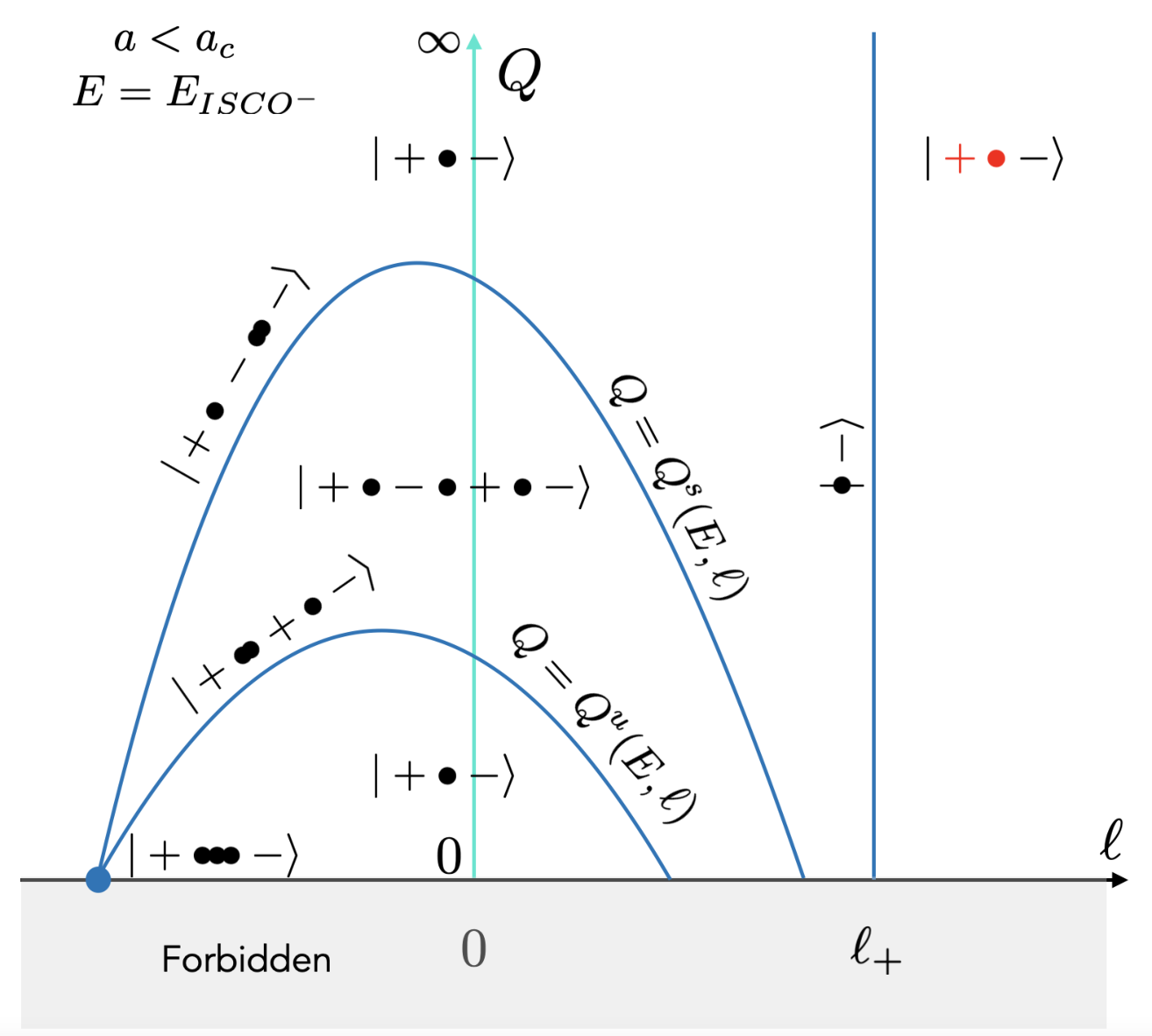
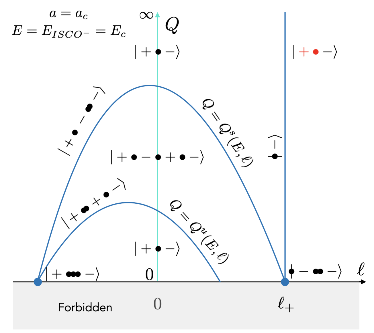
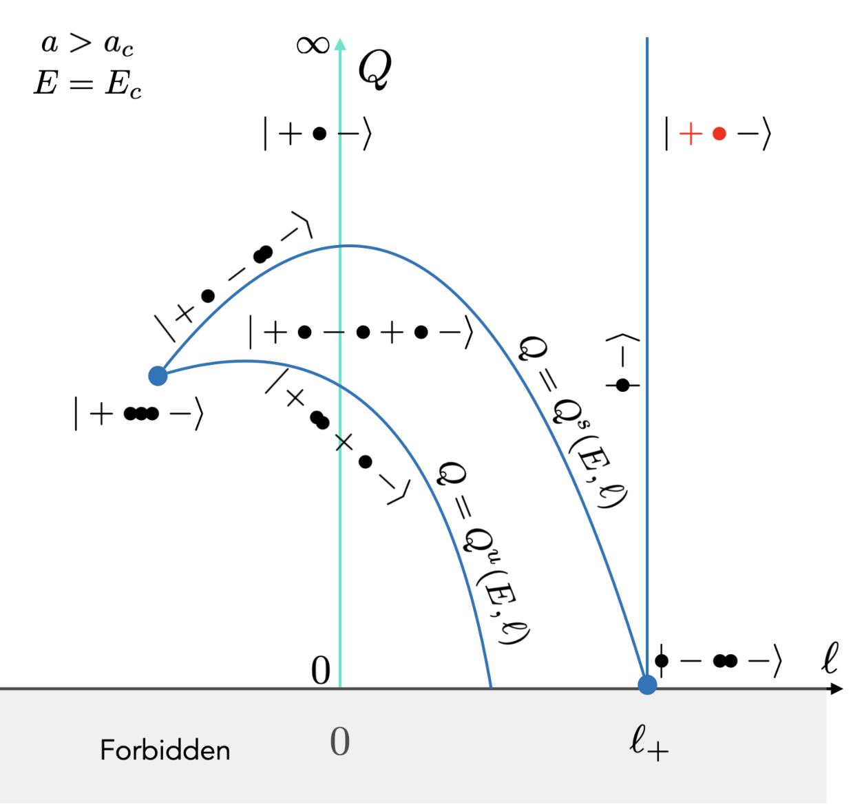
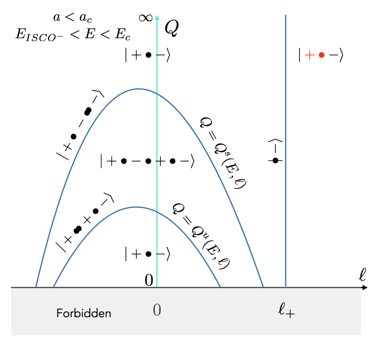
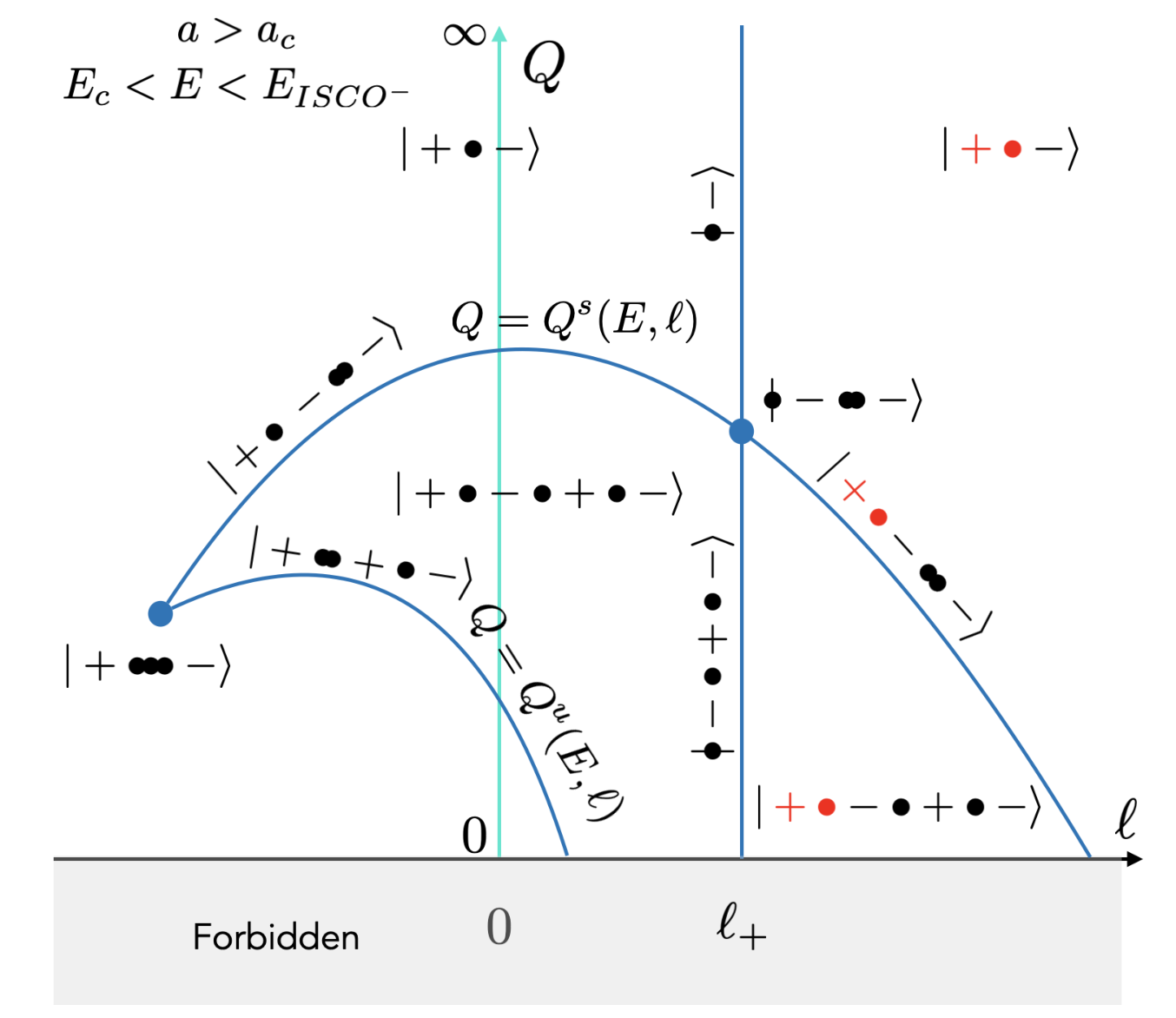
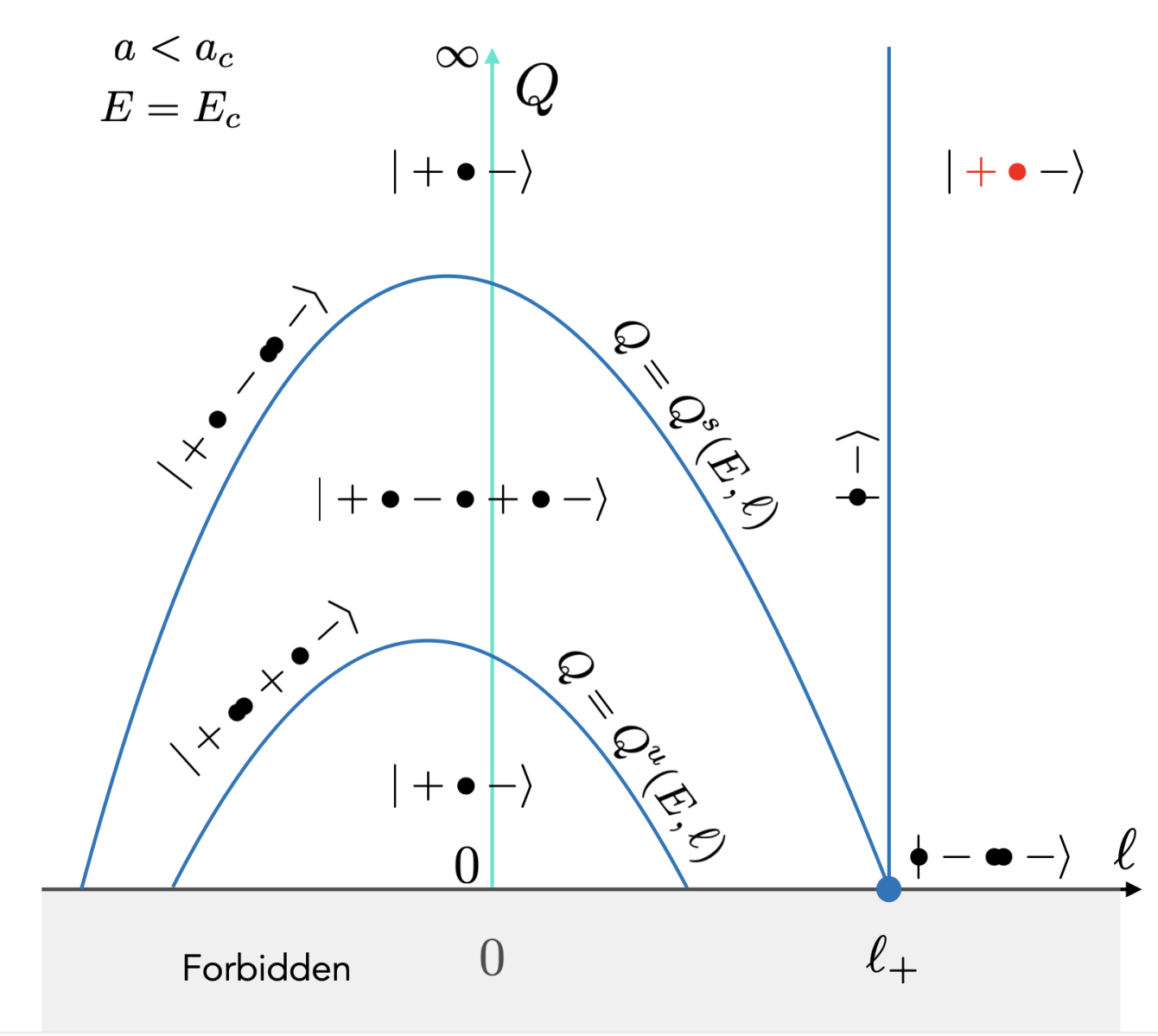
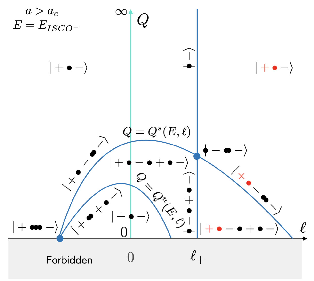
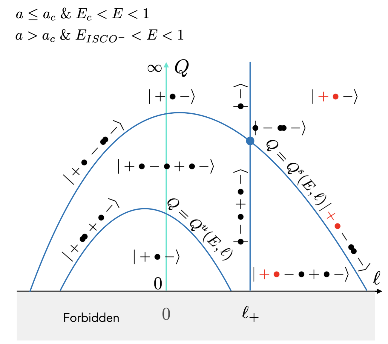
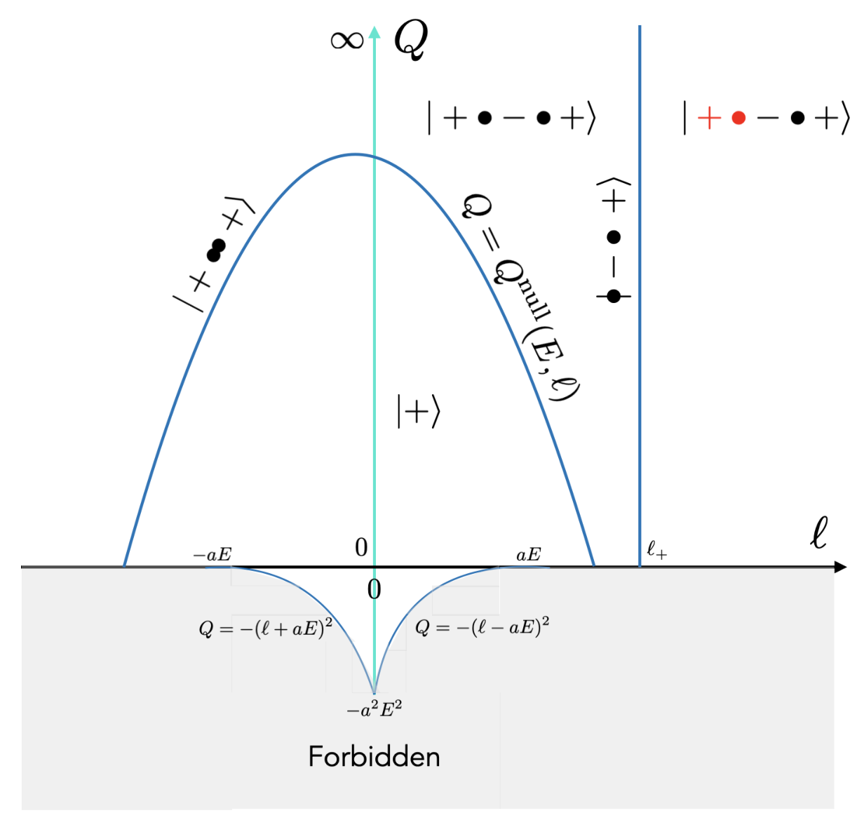
The final classification of radial motion of E<1E<1 timelike Kerr orbits can be found in Figure 7. The classification of radial motion of E>1E>1 orbits is shown in Figure 6. Moreover, we display the classification of radial motion of equatorial orbits in the (E,ℓ)(E,\ell) plane in Figure 8. As discussed in Section 2.2, in the case E>0E>0 and ℓ>ℓ+\ell>\ell_{+}, the trapped orbits are disallowed, and the root structures have the form |+∙⋯⟩|\hskip 2.0pt{\color[rgb]{1,0,0}+\bullet\cdots\rangle}. The final list of 11 qualitatively distinct geodesic orbit classes (sometimes evaluated on specific subcases) is given in Table 5 following the notations introduced for Schwarzschild in Appendix B. The 11 distinct geodesic orbit classes already appear around the Schwarzschild background.

Refer to caption
Refer to caption
Figure 6: Classification of radial motion of E>1E>1 timelike Kerr orbits (left) and E>0E>0 null orbits (right).
Refer to caption
Refer to caption
Refer to caption
Refer to caption
Refer to caption
Refer to caption
Refer to caption
Refer to caption
Refer to caption
Refer to caption
Refer to caption
Figure 7: Classification of radial motion of 0≤E<10\leq E<1 timelike Kerr orbits.
Refer to caption
Figure 8: Classification of radial motion of equatorial timelike Kerr orbits. Where ℓu\ell^{u} and ℓs\ell^{s} are defined in (4.39) and (4.40).
Root structure Energy range Radial range Name
Generic |+∙−⟩|+\bullet\hskip 2.0pt-\rangle 0≤E<10\leq E<1 r+≤r≤r1r_{+}\leq r\leq r_{1} 𝒯⁡(E,ℓ,Q)\mathcal{T}(E,\ell,Q)
|+∙−∙+∙−⟩|+\bullet-\bullet+\bullet\hskip 2.0pt-\rangle EISCO+<E<1E_{\text{ISCO}^{+}}<E<1 r+≤r≤r1r_{+}\leq r\leq r_{1} 𝒯⁡(E,ℓ,Q)\mathcal{T}(E,\ell,Q)
r2≤r≤r3r_{2}\leq r\leq r_{3} ℬ⁡(E,ℓ,Q)\mathcal{B}(E,\ell,Q)
|+⟩|+\rangle E≥1E\geq 1 r+≤r<∞r_{+}\leq r<\infty 𝒫⁡(E,ℓ,Q)\mathcal{P}(E,\ell,Q)
|+∙−∙+⟩|+\bullet-\bullet\hskip 2.0pt+\rangle E≥1E\geq 1 r+≤r≤r1r_{+}\leq r\leq r_{1} 𝒯⁡(E,ℓ,Q)\mathcal{T}(E,\ell,Q)
r2≤r<∞r_{2}\leq r<\infty 𝒟⁡(E,ℓ,Q)\mathcal{D}(E,\ell,Q)
Codimen- |∙−⟩|\hskip-7.0pt\bullet-\rangle 0≤E<10\leq E<1 ∅\emptyset ∅\emptyset
sion 1 |∙−∙+∙−⟩|\hskip-7.0pt\bullet-\bullet+\bullet-\rangle Ec<E<1E_{c}<E<1 r2≤r≤r3r_{2}\leq r\leq r_{3} ℬ⁡(E,ℓ+,Q)\mathcal{B}(E,\ell_{+},Q)
|+∙−∙∙−⟩|+\bullet-\bullet\hskip-5.0pt\bullet-\rangle EISCO+<E<1E_{\text{ISCO}^{+}}<E<1 r+≤r≤r1r_{+}\leq r\leq r_{1} 𝒯⁡(E,ℓ,Qs​(E,ℓ))\mathcal{T}(E,\ell,Q^{s}(E,\ell))
r=r2r=r_{2} 𝒮s​(E,ℓ)\mathcal{S}^{s}(E,\ell)
|+∙∙+∙−⟩|+\bullet\hskip-5.0pt\bullet+\bullet-\rangle EISCO+<E<1E_{\text{ISCO}^{+}}<E<1 r+≤r<r1r_{+}\leq r<r_{1} 𝒲​𝒯u​(E,ℓ)\mathcal{W}\mathcal{T}^{u}(E,\ell)
r=r1r=r_{1} 𝒮u​(E,ℓ)\mathcal{S}^{u}(E,\ell)
r1<r≤r2r_{1}<r\leq r_{2} ℋu​(E,ℓ)\mathcal{H}^{u}(E,\ell)
|+∙∙+⟩|+\bullet\hskip-5.0pt\bullet+\rangle E≥1E\geq 1 r+≤r<r1r_{+}\leq r<r_{1} 𝒲​𝒯u​(E,ℓ)\mathcal{W}\mathcal{T}^{u}(E,\ell)
r=r1r=r_{1} 𝒮u​(E,ℓ)\mathcal{S}^{u}(E,\ell)
r1<r<∞r_{1}<r<\infty 𝒲​𝒟u​(E,ℓ)\mathcal{W}\mathcal{D}^{u}(E,\ell)
|∙−∙+⟩|\hskip-7.0pt\bullet-\bullet+\rangle E≥1E\geq 1 r2≤r<∞r_{2}\leq r<\infty 𝒟⁡(E,ℓ+,Q)\mathcal{D}(E,\ell_{+},Q)
Codimen- |∙−∙∙−⟩|\hskip-7.0pt\bullet-\bullet\hskip-5.0pt\bullet\hskip 2.0pt-\rangle Ec≤E<1E_{c}\leq E<1 r=r2r=r_{2} 𝒮s​(E,ℓ+,Q)\mathcal{S}^{s}(E,\ell_{+},Q)
sion 2 |+∙∙∙−⟩|+\bullet\hskip-5.0pt\bullet\hskip-5.0pt\bullet\hskip 2.0pt-\rangle EISCO+≤E≤EISCO−E_{\text{ISCO}^{+}}\leq E\leq E_{\text{ISCO}^{-}} r+≤r<r1r_{+}\leq r<r_{1} 𝒲​𝒯I​S​S​O​(E)\mathcal{W}\mathcal{T}_{ISSO}(E)
r=r1r=r_{1} 𝒮I​S​S​O​(E)\mathcal{S}_{ISSO}(E)
Table 5: Taxonomy of the 11 qualitatively distinct classes of radial geodesic motion of timelike Kerr geodesics with E≥0E\geq 0. The locations of the roots are labeled in increasing order r1<r2<⋯r_{1}<r_{2}<\cdots. The four generic geodesic classes are the following: trapped orbits 𝒯⁡(E,ℓ,Q)\mathcal{T}(E,\ell,Q) originating from the white hole, turning back at finite radius and plunging into the black hole; bounded orbits ℬ⁡(E,ℓ,Q)\mathcal{B}(E,\ell,Q) oscillating between the turning points; plunging orbits (or outward directed orbits with initially negative radial velocity) 𝒫⁡(E,ℓ,Q)\mathcal{P}(E,\ell,Q) plunging into the black hole from infinity; deflecting orbits 𝒟⁡(E,ℓ,Q)\mathcal{D}(E,\ell,Q) coming from infinity and bouncing back to infinity. The seven nongeneric geodesic classes (such that at least one endpoint differs from a simple root, the horizon or infinity) are the following: the stable spherical orbits 𝒮s​(E,ℓ)\mathcal{S}^{s}(E,\ell), the innermost stable spherical orbits 𝒮I​S​S​O​(E)\mathcal{S}_{ISSO}(E), and the unstable spherical orbits 𝒮u​(E,ℓ)\mathcal{S}^{u}(E,\ell); the whirling trapped orbits 𝒲​𝒯u​(E,ℓ)\mathcal{W}\mathcal{T}^{u}(E,\ell) either originating from the white hole and asymptotically approaching the unstable spherical orbits or originating asymptotically from the unstable spherical orbits and plunging into the black hole; the homoclinic orbits ℋu​(E,ℓ)\mathcal{H}^{u}(E,\ell) originating from and approaching the unstable spherical orbits after bouncing on a turning point; the whirling deflecting orbits 𝒲​𝒟u​(E,ℓ)\mathcal{W}\mathcal{D}^{u}(E,\ell) asymptotically approaching the spherical orbits and infinity; the whirling trapped ISSO orbits 𝒲​𝒯I​S​S​O​(E)\mathcal{W}\mathcal{T}_{ISSO}(E) either originating from the white hole and asymptotically approaching the ISSO or originating asymptotically from the ISSO and plunging into the black hole. Note that when ℓ>ℓ+\ell>\ell_{+}, the trapped orbits become disallowed, which we denote as |+∙⋯|+\bullet\cdots ↦\mapsto |+∙⋯|{\color[rgb]{1,0,0}+\bullet}\cdots.

3.6 Null geodesics

The classification of radial motion for null geodesics can be simply obtained from the timelike classification in the limit E→∞E\rightarrow\infty. The corresponding phase space is provided in Figure 6. In this section, we briefly review the classification of radial root structures as performed by Gralla and Lupsasca [60] (restricting our analysis to r>r+r>r_{+}) and extend it, using the constraints on motion within the ergoregion discussed in Section 2.2, to the classification of allowed radial motion.

In this subsection we assume no mass, μ=0\mu=0, and positive energy E>0E>0. It is convenient to define

λ=ℓE,η=QE2.\lambda=\frac{\ell}{E},\qquad\eta=\frac{Q}{E^{2}}. (3.63)

The radial potential is then given by

R⁡(r)=r4+(a2−η−λ2)​r2+2​(a2+η−2​a​λ+λ2)​r−a2​η.R(r)=r^{4}+(a^{2}-\eta-\lambda^{2})r^{2}+2(a^{2}+\eta-2a\lambda+\lambda^{2})r-a^{2}\eta. (3.64)

The positivity bound (2.1) reduces to

η≥{0 for ​|λ|≥a;−(|λ|−a)2 for ​|λ|<a.\eta\geq\left\{\begin{array}[]{ll}0&\text{ for }|\lambda|\geq a;\\ -(|\lambda|-a)^{2}&\text{ for }|\lambda|<a.\end{array}\right. (3.65)

The only double root that may obey the positivity bound is

η\displaystyle\eta =\displaystyle= η∗​(r∗)=−r∗3​(−4​a2+r∗​(r∗−3)2)a2​(r∗−1)2,\displaystyle\eta_{*}(r_{*})=-\frac{r_{*}^{3}(-4a^{2}+r_{*}(r_{*}-3)^{2})}{a^{2}(r_{*}-1)^{2}},
λ\displaystyle\lambda =\displaystyle= λ∗​(r∗)=r∗2​(r∗−3)+a2​(r∗+1)a⁡(1−r∗).\displaystyle\lambda_{*}(r_{*})=\frac{r_{*}^{2}(r_{*}-3)+a^{2}(r_{*}+1)}{a(1-r_{*})}.

In the radial range where |λ∗​(r∗)|<a|\lambda_{*}(r_{*})|<a, we have η∗​(r∗)>0\eta_{*}(r_{*})>0. The bound for double roots therefore reduces to η∗​(r∗)≥0\eta_{*}(r_{*})\geq 0, which amounts to

rp​h+≤r∗≤rp​h−,r_{ph^{+}}\leq r_{*}\leq r_{ph^{-}}, (3.66)

with

rp​h+\displaystyle r_{ph^{+}} =\displaystyle= 2+2​cos⁡[23​arccos⁡a+4​π3],\displaystyle 2+2\cos[\frac{2}{3}\arccos a+\frac{4\pi}{3}],
rp​h−\displaystyle r_{ph^{-}} =\displaystyle= 2+2​cos⁡[23​arccos⁡a].\displaystyle 2+2\cos[\frac{2}{3}\arccos a].

The angular momentum obeys λp​h−≤λ∗≤λp​h+\lambda_{ph^{-}}\leq\lambda_{*}\leq\lambda_{ph^{+}} with λp​h±=λ∗​(rp​h±)\lambda_{ph^{\pm}}=\lambda_{*}(r_{ph^{\pm}}). At the horizon, R=(2​r+−a​λ)2≥0R=(2r_{+}-a\lambda)^{2}\geq 0, and there is a root touching the horizon if and only if

λ=λ+≡2​r+a.\lambda=\lambda_{+}\equiv\frac{2r_{+}}{a}. (3.67)

One has λp​h+<λ+\lambda_{ph+}<\lambda_{+} for 0<a<10<a<1. Since λ∗​(r∗)\lambda_{*}(r_{*}) is monotonic between rp​h+≤r∗≤rp​h−r_{ph+}\leq r_{*}\leq r_{ph-}, one can define an inverse function r∗​(λ)r_{*}(\lambda), and the double root is described by

Q=Qnull​(E,ℓ)≡E2​ηnull​(ℓE),ηnull​(ℓE)≡η∗​(r∗​(λ)).Q=Q^{\text{null}}(E,\ell)\equiv E^{2}\eta^{\text{null}}(\frac{\ell}{E}),\qquad\eta^{\text{null}}(\frac{\ell}{E})\equiv\eta_{*}(r_{*}(\lambda)). (3.68)

The function ηnull​(λ)\eta^{\text{null}}(\lambda) reaches a maximum at λ=−2​a\lambda=-2a with ηnull​(−2​a)=27\eta^{\text{null}}(-2a)=27 independently of aa. The corresponding radius is r∗=3r_{*}=3, which coincides with the photon sphere of the Schwarzschild solution.

Now, the bound (2.26) rules out trapped orbits within the ergoregion. This implies that the root structure |+∙−∙+⟩|+\bullet-\bullet\hskip 3.0pt+\rangle for ℓ>ℓ+​(E)=E/Ω+\ell>\ell_{+}(E)=E/\Omega_{+} contains disallowed trapped orbits, |+∙−∙+⟩{|\;{\color[rgb]{1,0,0}+\;\bullet}-\bullet\hskip 3.0pt+\rangle}. This condition was not analyzed in [60]. This completes the result on the classification of radial root structures by the classification of allowed radial motion. The final root structure is depicted in Figure 6.

4 Classification of radial geodesic motion within the ergoregion

In the previous section, we did not consider the exact location of the ergosphere in the classification of radial root systems. In the following, we will introduce the location of the ergosphere, denoted with the symbol )), discuss where it appears within each root system, and present the classification of root systems and radial geodesic motion within the ergoregion, i.e., between the horizon and the ergosphere. We will start with a complete classification of such root systems and corresponding allowed radial geodesic motion on the equator, which will lead to the identification of six distinguished values of the Kerr angular momentum aa. We will then briefly discuss the nonequatorial radial motion and finally derive the classification of radial motion within the near-horizon region of near-extremal Kerr.

4.1 Root structures and allowed radial motion on the equator

We consider the root structures with roots between the horizon and the ergosphere. There can be maximally three such roots for E2≠1E^{2}\neq 1 and maximally two such roots for E2=1E^{2}=1. The root structures have the generic form |+⋯)⋯⟩|+\cdots)\cdots\rangle when ℓ≠ℓ+​(E)=E/Ω+\ell\neq\ell_{+}(E)=E/\Omega_{+} or the particular form |∙−⋯)⋯⟩{|\hskip-7.0pt\bullet-\cdots)\cdots\rangle} when ℓ=ℓ+​(E)\ell=\ell_{+}(E). The root structure outside the ergosphere can be ignored for the classification within the ergoregion, but it is useful as a comparison with our earlier classification.

Since

rergo​(θ,a)≤2<1+2≤r∗(0)​(a)r_{\text{ergo}}(\theta;a)\leq 2<1+\sqrt{2}\leq r_{*}^{(0)}(a) (4.1)

where r∗(0)r_{*}^{(0)} is defined below (3.55), all root structures with a double root have necessarily negative angular momentum, ℓ<0\ell<0 for E<0E<0 and positive ℓ>0\ell>0 for E>0E>0. By continuity, root structures with sign​(ℓ)≠sign​(E)\text{sign}(\ell)\neq\text{sign}(E) and with two simple roots within the ergosphere are also discarded.

From now on, we will only discuss the equatorial case θ=π2\theta=\frac{\pi}{2} where, accordingly, Q=0Q=0 and rergo=2r_{\text{ergo}}=2. The potential has a root r=0r=0 which can be factored out. The relevant potential becomes

R0​(r)=(E2−1)​r3+2​r2+(a2​(E2−1)−ℓ2)​r+2​(ℓ−a​E)2.R_{0}(r)=(E^{2}-1)r^{3}+2r^{2}+(a^{2}(E^{2}-1)-\ell^{2})r+2(\ell-aE)^{2}. (4.2)

We consider only nonvanishing energy orbits E≠0E\neq 0 in Kerr with 0<a≤10<a\leq 1.

Inequalities

The inequalities (2.24)–(2.25) reduce for E<0E<0 to

(2−r)​ℓ≤2​a​E<0.(2-r)\ell\leq 2aE<0. (4.3)

Negative energy orbits that reach the ergosphere r=2r=2 are discarded. Moreover, all timelike orbits within the equatorial ergoregion have a negative angular momentum. The inequality (4.3) can be solved by

ℓ≤ℓϕ​(E,r)≡2​a​E2−r\ell\leq\ell_{\phi}(E,r)\equiv\frac{2aE}{2-r} (4.4)

for negative energy orbits in the ergoregion. Since r+≤r<2r_{+}\leq r<2, it implies, in particular, for all orbits with E<0E<0 that

ℓ≤2​a​E2−r≤2​a​E2−r+=2​r+a​E=EΩ+.\ell\leq\frac{2aE}{2-r}\leq\frac{2aE}{2-r_{+}}=\frac{2r_{+}}{a}E=\frac{E}{\Omega_{+}}. (4.5)

The thermodynamic bound (2.26) is therefore obeyed for all orbits with E<0E<0. The upper bound ℓ=ℓ+​(E)\ell=\ell_{+}(E) corresponds to root structures with one root at the horizon.

The inequalities (2.24)–(2.25) reduce for E>0E>0 to

ℓ<ℓt​(E,r)≡r3+r​a2+2​a22​a​E.\ell<\ell_{t}(E,r)\equiv\frac{r^{3}+ra^{2}+2a^{2}}{2a}E. (4.6)

For timelike geodesics, we have uμ​uμ<0u_{\mu}u^{\mu}<0, which also implies the independent inequalities

−gt​ϕ−sin⁡θ​Δgϕ​ϕ<d​ϕd​t<−gt​ϕ+sin⁡θ​Δgϕ​ϕ\frac{-g_{t\phi}-\sin\theta\sqrt{\Delta}}{g_{\phi\phi}}<\frac{d\phi}{dt}<\frac{-g_{t\phi}+\sin\theta\sqrt{\Delta}}{g_{\phi\phi}} (4.7)

in the ergoregion. Here, d​ϕd​t=−(ℓEgt​t+gt​ϕ)/(ℓEgt​ϕ+gϕ​ϕ)\frac{d\phi}{dt}=-(\frac{\ell}{E}g_{tt}+g_{t\phi})/(\frac{\ell}{E}g_{t\phi}+g_{\phi\phi}). The bound (4.7) becomes

0<2​a−r​Δr3+a2​(r+2)<d​ϕd​t<2​a+r​Δr3+a2​(r+2).0<\frac{2a-r\sqrt{\Delta}}{r^{3}+a^{2}(r+2)}<\frac{d\phi}{dt}<\frac{2a+r\sqrt{\Delta}}{r^{3}+a^{2}(r+2)}. (4.8)

where d​ϕd​t=−(ℓEgt​t+gt​ϕ)/(ℓEgt​ϕ+gϕ​ϕ)\frac{d\phi}{dt}=-(\frac{\ell}{E}g_{tt}+g_{t\phi})/(\frac{\ell}{E}g_{t\phi}+g_{\phi\phi}). We define the quantities

ℓ(1,2)​(E,r)=2​a∓r​Δ2−r​E.\displaystyle\ell^{(1,2)}(E,r)=\frac{2a\mp r\sqrt{\Delta}}{2-r}E. (4.9)

For E<0E<0, they obey ℓ(2)​(E,r)<ℓϕ​(E,r)<ℓ(1)​(E,r)\ell^{(2)}(E,r)<\ell_{\phi}(E,r)<\ell^{(1)}(E,r), while for E>0E>0 they obey ℓ(1)​(E,r)<ℓt​(E,r)<ℓ(2)​(E,r)\ell^{(1)}(E,r)<\ell_{t}(E,r)<\ell^{(2)}(E,r). We deduce from (4.8) that for E<0E<0 the angular momentum should satisfy

ℓ<ℓ(2)​(E,r)<0\ell<\ell^{(2)}(E,r)<0 (4.10)

and Eq. (4.4) is automatically obeyed, while for E>0E>0 the angular momentum should satisfy

ℓ<ℓ(1)​(E,r).\ell<\ell^{(1)}(E,r). (4.11)

and Eq. (4.6) is automatically obeyed.

Finally, we impose that the potential R0​(r)R_{0}(r) is non-negative. This condition can be solved for ℓ\ell as

ℓ≥ℓ0(1)​(E,r)orℓ≤ℓ0(2)​(E,r)\ell\geq\ell_{0}^{(1)}(E,r)\quad\text{or}\quad\ell\leq\ell_{0}^{(2)}(E,r) (4.12)

within the ergoregion, where we have defined

ℓ0(1,2)​(E,r)=2​a​E±r⁡(2+(E2−1)​r)​Δ​(r)2−r.\ell_{0}^{(1,2)}(E,r)=\frac{2aE\pm\sqrt{r(2+(E^{2}-1)r)\Delta(r)}}{2-r}. (4.13)

From the definition (4.13), we can directly derive that ℓ0(1)​(E,r)≥ℓ0(2)​(E,r)\ell_{0}^{(1)}(E,r)\geq\ell_{0}^{(2)}(E,r). Moreover, for E>0E>0, ℓ0(1)​(E,r)+ℓ0(2)​(E,r)≥2​ℓ+​(E)\ell_{0}^{(1)}(E,r)+\ell_{0}^{(2)}(E,r)\geq 2\ell_{+}(E), which implies for E>0E>0

ℓ0(1)​(E,r)≥ℓ+​(E),\ell_{0}^{(1)}(E,r)\geq\ell_{+}(E), (4.14)

while for E<0E<0, ℓ0(1)​(E,r)+ℓ0(2)​(E,r)≤2​ℓ+​(E)\ell_{0}^{(1)}(E,r)+\ell_{0}^{(2)}(E,r)\leq 2\ell_{+}(E) which

ℓ0(2)​(E,r)≤ℓ+​(E).\ell_{0}^{(2)}(E,r)\leq\ell_{+}(E). (4.15)

When E<0E<0, we find

ℓ0(2)​(E,r)<ℓ(2)​(E,r)<ℓ0(1)​(E,r).\ell_{0}^{(2)}(E,r)<\ell^{(2)}(E,r)<\ell_{0}^{(1)}(E,r). (4.16)

When E>0E>0, we find

ℓ0(2)​(E,r)<ℓ(1)​(E,r)<ℓ0(1)​(E,r).\ell_{0}^{(2)}(E,r)<\ell^{(1)}(E,r)<\ell_{0}^{(1)}(E,r). (4.17)

Combining with Eqs. (4.10) and (4.11), the bound becomes

ℓ≤ℓ0(2)​(E,r)\ell\leq\ell_{0}^{(2)}(E,r) (4.18)

for both positive and negative energy equatorial orbits within the ergoregion. This is the final inequality that supersedes all previous inequalities. In particular, for plunging orbits, the bound has to be obeyed at r=r+r=r_{+}. Since ℓ0(2)​(E,r+)=2​r+a​E=ℓ+​(E)\ell^{(2)}_{0}(E,r_{+})=\frac{2r_{+}}{a}E=\ell_{+}(E), we obtain for all trapped orbits

ℓ≤ℓ+​(E).\ell\leq\ell_{+}(E). (4.19)

From (4.18) and (4.15), this bound is moreover obeyed for any E<0E<0 orbit.

Both prograde and retrograde orbits are therefore allowed for E>0E>0. The condition (4.18) and (4.19) impose constraints which will be discussed below. In the limit E=0E=0, the bound (4.18) reduces to

ℓ≤−r​Δ2−r<0,\ell\leq-\sqrt{\frac{r\Delta}{2-r}}<0, (4.20)

and orbits are retrograde as they should.

From (4.19), root structures of the form |+∙−)|+\bullet\hskip 2.0pt-) for ℓ>ℓ+​(E)\ell>\ell_{+}(E) will be denoted as |+∙−)|{\color[rgb]{1,0,0}\hskip 2.0pt+\hskip 2.0pt\bullet}\hskip 2.0pt-).

A corollary from the inequalities (4.14) and (4.12) is that for all root structures with E>0E>0 and ℓ≤ℓ+​(E)\ell\leq\ell_{+}(E), the region R0​(r)≥0R_{0}(r)\geq 0 necessarily obeys the bound (4.18). Therefore, all motion denoted as ++ in root structures with ℓ≤ℓ+​(E)\ell\leq\ell_{+}(E) and E>0E>0 are allowed. Root structures such as |+∙−∙+)|+\bullet-\bullet\hskip 2.0pt+) for ℓ>ℓ+​(E)\ell>\ell_{+}(E) and E>0E>0 require more care. From (4.19), one deduces that the plunging orbits are disallowed. However, the orbits entering and escaping the ergoregion are not constrained by this inequality. We will check that such orbits obey the bound (4.18). We will therefore denote orbits with E>0E>0 and ℓ>ℓ+​(E)\ell>\ell_{+}(E) as |+∙−∙+)|{\color[rgb]{1,0,0}\hskip 2.0pt+\hskip 2.0pt\bullet}-\bullet\hskip 2.0pt+).

Special values of aa. Roots at the horizon or at the ergosphere.

In the following, we will define six particular values of aa, which we will order in increasing values as

0<ac(1)<ac(2)<ac(3)<ac(4)<ac(5)<ac(6)<10<a_{c}^{(1)}<a_{c}^{(2)}<a_{c}^{(3)}<a_{c}^{(4)}<a_{c}^{(5)}<a_{c}^{(6)}<1 (4.21)

where distinctive root structures will emerge.

We define the angular momentum ℓ=ℓe​(E,a)\ell=\ell_{e}(E;a) such that

R0​(rergo)=0.R_{0}(r_{\text{ergo}})=0. (4.22)

At the equator, the solution is unique and given by

ℓ=ℓe​(E,a)≡(4+2​a2)​E2−a22​a​E.\ell=\ell_{e}(E;a)\equiv\frac{(4+2a^{2})E^{2}-a^{2}}{2aE}. (4.23)

For such angular momentum, the local root structure is given by ⋯)∙⋯{\cdots)\hskip-7.0pt\bullet\cdots}. For E<0E<0 only, the constraint ℓe​(E,a)<0\ell_{e}(E;a)<0 is obeyed only for

E<−a4+2​a2.E<-\frac{a}{\sqrt{4+2a^{2}}}. (4.24)

A double root at the ergosphere can occur only for a>ac(1)a>a_{c}^{(1)}, where

ac(1)≡12≈0.707107.a_{c}^{(1)}\equiv\frac{1}{\sqrt{2}}\approx 0.707107. (4.25)

The double root at the ergosphere corresponding to ⋯)∙∙⋯{\cdots)\hskip-9.0pt\bullet\hskip-4.0pt\bullet\cdots} then occurs when

E\displaystyle E =\displaystyle= Ee±​(a)≡±a2​2​a−1,\displaystyle E^{\pm}_{e}(a)\equiv\pm\frac{a}{2\sqrt{\sqrt{2}a-1}}, (4.26)
ℓ\displaystyle\ell =\displaystyle= ℓe​(Ee±​(a),a)=±2−2​a+a222​a−1.\displaystyle\ell_{e}(E^{\pm}_{e}(a);a)=\pm\frac{2-\sqrt{2}a+\frac{a^{2}}{2}}{\sqrt{\sqrt{2}a-1}}. (4.27)

We have sign​(ℓe​(Ee±​(a),a))=sign​(E)\text{sign}(\ell_{e}(E^{\pm}_{e}(a);a))=\text{sign}(E) for a>ac(1)a>a_{c}^{(1)}, in accordance with our discussion that only orbits with sign​(ℓ)=sign​(E)\text{sign}(\ell)=\text{sign}(E) occur in the presence of double roots within the ergoregion. With respect to our discussion in Section 3.5, we have Ee±​(a)=±E(2)​(2)E^{\pm}_{e}(a)=\pm E^{(2)}(2), where E(2)​(r∗)E^{(2)}(r_{*}) is defined in (3.48). The function Ee​(a)E_{e}(a) crosses E=±1E=\pm 1 at a=ac(2)a=a_{c}^{(2)}, where

ac(2)≡2​(2−1)≈0.828427.a_{c}^{(2)}\equiv 2(\sqrt{2}-1)\approx 0.828427. (4.28)

The function ℓe​(E,a)\ell_{e}(E;a) crosses ℓ+​(E,a)\ell_{+}(E;a) defined in (3.9) only for a>ac(3)a>a_{c}^{(3)} at

E=E+e±​(a)≡±a2​a2−2​1−a2E=E^{\pm}_{+e}(a)\equiv\pm\frac{a}{\sqrt{2}\sqrt{a^{2}-2\sqrt{1-a^{2}}}} (4.29)

where

ac(3)≡2​(2−1)≈0.91018.a_{c}^{(3)}\equiv\sqrt{2(\sqrt{2}-1)}\approx 0.91018. (4.30)

The root structures |∙−)∙{|\hskip-7.0pt\bullet-)\hskip-4.0pt\bullet} with one root at the horizon and one root at the ergosphere therefore occur for EE given by (4.29) and ℓ\ell given by

ℓ=ℓ+e±​(a)≡±2​(1+1−a2)a2−2​1−a2.\ell=\ell^{\pm}_{+e}(a)\equiv\pm\frac{\sqrt{2}(1+\sqrt{1-a^{2}})}{\sqrt{a^{2}-2\sqrt{1-a^{2}}}}. (4.31)

The energy (4.29) reaches E2=1E^{2}=1 at a=ac(5)a=a_{c}^{(5)}, where

ac(5)≡2​5−2≈0.971737.a_{c}^{(5)}\equiv 2\sqrt{\sqrt{5}-2}\approx 0.971737. (4.32)

The special root structures |∙−∙∙−⟩{|\hskip-7.0pt\bullet-\bullet\hskip-6.0pt\bullet\hskip 2.0pt-\rangle} occur at the equator for ℓ=ℓ+​(E,a)\ell=\ell_{+}(E;a) and E=±Ec​(a)E=\pm E_{c}(a) where Ec​(a)E_{c}(a) is given in (3.15). We have ±Ec​(a)=Ee±​(a)\pm E_{c}(a)=E^{\pm}_{e}(a) at a=ac(6)a=a_{c}^{(6)}, where

ac(6)=23​Z−24​Z−1≈0.996175,Z≡31/3​(9+7​33)1/3.a_{c}^{(6)}=\frac{2}{\sqrt{3}}\sqrt{Z-24Z^{-1}}\approx 0.996175,\qquad Z\equiv 3^{1/3}(9+7\sqrt{33})^{1/3}. (4.33)

For that special value of aa, ℓ=ℓ+​(E,a)\ell=\ell_{+}(E;a) and E=Ee±​(a)E=E^{\pm}_{e}(a), the double root is at the ergosphere, leading to the root structure |∙−∙)∙−⟩{|\hskip-7.0pt\bullet-\bullet\hskip-4.0pt)\hskip-5.0pt\bullet\hskip 0.0pt-\rangle}.

Finally, a triple root at the ergosphere occurs for the particular value a=ac(4)a=a_{c}^{(4)}, where

ac(4)≡2​23≈0.942809.a_{c}^{(4)}\equiv\frac{2\sqrt{2}}{3}\approx 0.942809. (4.34)

It is also the unique solution to the equation rI​S​C​O+​(a)=2r_{ISCO^{+}}(a)=2. The unique triple root structure at the ergosphere |+∙)∙∙{|+\bullet\hskip-2.0pt)\hskip-7.0pt\bullet\hskip-4.0pt\bullet} therefore occurs at the two special values [sign​(E)=sign​(ℓ)\text{sign}(E)=\text{sign}(\ell)],

E=±23,ℓ=±103​3,a=ac(4).E=\pm\sqrt{\frac{2}{3}},\qquad\ell=\pm\frac{10}{3\sqrt{3}},\qquad a=a_{c}^{(4)}. (4.35)

The summary of the six distinguished values ac(i)a_{c}^{(i)} of the Kerr angular momentum is given in Table 6.

ac(1)a_{c}^{(1)} ac(2)a_{c}^{(2)} ac(3)a_{c}^{(3)} ac(4)a_{c}^{(4)} ac(5)a_{c}^{(5)} ac(6)a_{c}^{(6)}
12\frac{1}{\sqrt{2}} 2​(2−1)2(\sqrt{2}-1) 2​(2−1)\sqrt{2(\sqrt{2}-1)} 2​23\frac{2\sqrt{2}}{3} 2​5−22\sqrt{\sqrt{5}-2} 23​Z−24​Z−1\frac{2}{\sqrt{3}}\sqrt{Z-24Z^{-1}}
0.707 0.828 0.910 0.943 0.972 0.996
Table 6: Exact and approximate values of ac(i)a_{c}^{(i)}.
Double roots.

So far we only defined the root structures with a double root located on the ergosphere. More generally, the double roots occur for equatorial orbits for E=±E(2)​(r∗)E=\pm E^{(2)}(r_{*}) as given by (3.48) and ℓ=±ℓb​(E(2)​(r∗),r∗)\ell=\pm\ell_{\text{b}}(E^{(2)}(r_{*}),r_{*}) as given by (3.38) in terms of the radius of the double root r∗r_{*}. We can rewrite these equations as

E=E±​(r∗,a)≡±(r∗−2)​r∗+ar∗3/2​((r∗−3)​r∗1/2+2​a),ℓ=ℓ±​(r∗,a)≡±r∗2−2​a​r∗+a2r∗3/2​((r∗−3)​r∗1/2+2​a).E=E^{\pm}(r_{*};a)\equiv\pm\frac{(r_{*}-2)\sqrt{r_{*}}+a}{\sqrt{r_{*}^{3/2}((r_{*}-3)r_{*}^{1/2}+2a)}},\quad\ell=\ell^{\pm}(r_{*};a)\equiv\pm\frac{r_{*}^{2}-2a\sqrt{r_{*}}+a^{2}}{\sqrt{r_{*}^{3/2}((r_{*}-3)r_{*}^{1/2}+2a)}}. (4.36)

Such double roots may lie in the ergoregion for a≥ac(1)a\geq a_{c}^{(1)}. We have

2​a​E−​(r∗,a)2−r∗−ℓ−​(r∗,a)=−r∗1/4​Δ​(r∗)(2−r∗)​r∗3/2−3​r∗+2​a<0.\frac{2aE^{-}(r_{*};a)}{2-r_{*}}-\ell^{-}(r_{*};a)=-\frac{r_{*}^{1/4}\Delta(r_{*})}{(2-r_{*})\sqrt{r_{*}^{3/2}-3\sqrt{r_{*}}+2a}}<0. (4.37)

Therefore, negative energy orbits with double roots are disallowed by the condition (2.27). This implies, in particular, that no circular orbit with negative energy is allowed in the ergoregion. By continuity, no bounded motion is allowed and only trapped orbits are allowed. The bound (4.19) therefore applies for any orbit with E<0E<0.

On the other hand, we have identically

ℓ0(2)​(E+​(r∗,a),r∗)=ℓ+​(r∗,a),\displaystyle\ell^{(2)}_{0}(E^{+}(r_{*};a),r_{*})=\ell^{+}(r_{*};a), (4.38)

where ℓ0(2)\ell_{0}^{(2)} was defined in (4.13). Therefore, positive energy orbits with double roots are allowed by the condition (4.18) (for a≥ac(1)a\geq a_{c}^{(1)}). In particular, circular orbits with positive energy are allowed in the ergoregion. However, since r∗(2)≥3r_{*}^{(2)}\geq 3, circular orbits with ℓ<0\ell<0 and E>0E>0 do not appear in the ergoregion.

The triple root occurs at the ISCO radius r∗=rI​S​C​O±r_{*}=r_{ISCO^{\pm}}, which has sign​(E)=sign​(ℓ)=±1\text{sign}(E)=\text{sign}(\ell)=\pm 1. In the range r∗(1)<r∗<rI​S​C​O±r_{*}^{(1)}<r_{*}<r_{ISCO^{\pm}}, one can invert E±​(r∗)E^{\pm}(r_{*}) to r∗u​(E)r_{*}^{u}(E) and define

ℓu​(E,a)≡ℓ±​(r∗u​(E)).\ell^{u}(E;a)\equiv\ell^{\pm}(r^{u}_{*}(E)). (4.39)

As discussed in Section 3.5, the corresponding double root is unstable: the root structure takes the local form ⋯+∙∙+…{\cdots+\bullet\hskip-6.0pt\bullet+\dots}. Since we only consider the ergoregion in this section, we will only define ℓu\ell^{u} when r∗​(E)≤2r_{*}(E)\leq 2. In the range rI​S​C​O±<r∗<∞r_{ISCO^{\pm}}<r_{*}<\infty, one can invert E±​(r∗)E^{\pm}(r_{*}) to r∗s​(E)r_{*}^{s}(E) and define

ℓs​(E,a)≡ℓ±​(r∗s​(E)).\ell^{s}(E;a)\equiv\ell^{\pm}(r^{s}_{*}(E)). (4.40)

The corresponding double root is stable: the root structure takes the local form ⋯−∙∙−⋯{\cdots-\bullet\hskip-6.0pt\bullet-\cdots}. Since we only consider the ergoregion in this section, we will only define ℓs\ell^{s} when r∗s​(E)≤2r^{s}_{*}(E)\leq 2.

Let us discuss the root systems which admit both a root at the ergosphere and double roots. This occurs at the intersection of the lines ℓ=ℓe​(E,a)\ell=\ell_{e}(E;a) and ℓ=\ell= either ℓu​(E,a)\ell^{u}(E;a) or ℓs​(E,a)\ell^{s}(E;a). Algebraically, it amounts to find the roots r∗r_{*} of ℓ+​(r∗,a)=ℓe​(E+​(r∗),a)\ell^{+}(r_{*};a)=\ell_{e}(E^{+}(r_{*});a). After analysis, there are three main cases depending upon the value of aa.

  • •

    For a≤ac(1)a\leq a_{c}^{(1)}, there is no solution within the ergoregion. Instead, there is one real solution r∗=2​r+a2−1>2r_{*}=\frac{2r_{+}}{a^{2}}-1>2 intersecting ℓ=ℓs\ell=\ell^{s}, which corresponds to the root structure |+∙)−∙∙−⟩|+\bullet\hskip-6.0pt)-\bullet\hskip-4.0pt\bullet-\rangle.

  • •

    For ac(1)<a≤ac(4)a_{c}^{(1)}<a\leq a_{c}^{(4)}, there is the solution at the ergosphere r∗=2r_{*}=2 intersecting ℓ=ℓu\ell=\ell^{u}, corresponding to the root structure |+∙)∙+⟩{|+\bullet\hskip-4.0pt)\hskip-5.0pt\bullet+\rangle}. This structure degenerates to the triple root at the ergosphere |+∙)∙∙−⟩{|+\bullet\hskip-2.0pt)\hskip-7.0pt\bullet\hskip-4.0pt\bullet-\rangle} at a=ac(4)a=a_{c}^{(4)}. The other real solution r∗=2​r+a2−1r_{*}=\frac{2r_{+}}{a^{2}}-1 is outside the ergosphere for a<ac(4)a<a_{c}^{(4)}. In that case the curve ℓ=ℓe\ell=\ell_{e} intersects ℓ=ℓs\ell=\ell^{s}, and the root structure is |+∙)−∙∙−⟩|+\bullet\hskip-6.0pt)-\bullet\hskip-4.0pt\bullet-\rangle.

  • •

    For ac(4)<a≤1a_{c}^{(4)}<a\leq 1, there is the new solution r∗=2​r+a2−1r_{*}=\frac{2r_{+}}{a^{2}}-1 intersecting ℓ=ℓu\ell=\ell^{u}, but which now corresponds to the root structure |+∙∙+)∙|+\bullet\hskip-6.0pt\bullet+\hskip 2.0pt)\hskip-4.0pt\bullet, and there is still the solution r∗=2r_{*}=2 intersecting now ℓ=ℓs\ell=\ell^{s}, which corresponds to the root structure |+∙−∙)∙|+\bullet-\bullet\hskip-4.0pt)\hskip-2.0pt\bullet for a≠ac(6)a\neq a_{c}^{(6)}. The latter solution degenerates to |∙−∙)∙{|\hskip-7.0pt\bullet-\bullet\hskip-4.0pt)\hskip-2.0pt\bullet} for a=ac(6)a=a_{c}^{(6)}.

Construction of the phase diagrams.

We defined four relevant curves to classify the root structures:

  • •

    ℓ=ℓ+​(E)\ell=\ell_{+}(E). The root structure takes the local form |∙−⋯{|\hskip-7.0pt\bullet-\cdots}.

  • •

    ℓ=ℓe​(E)\ell=\ell_{e}(E). The root structure takes the local form ⋯)∙{\cdots)\hskip-4.0pt\bullet}.

  • •

    ℓ=ℓu​(E)\ell=\ell^{u}(E). The root structure takes the local form ⋯+∙∙+…{\cdots+\bullet\hskip-5.0pt\bullet+\dots}.

  • •

    ℓ=ℓs​(E)\ell=\ell^{s}(E). The root structure takes the local form ⋯−∙∙−⋯{\cdots-\bullet\hskip-5.0pt\bullet-\cdots}.

The pattern of intersection of these lines depends upon the value of the spin aa relatively to the special values (4.21). Moreover, one has to impose the constraints (4.18)–(4.19), which qualitatively differ for E>0E>0 and E<0E<0 orbits. We, therefore, discuss the phase spaces for E>0E>0 and E<0E<0 separately.

Phase diagram for E>0E>0.

The rich phase diagram for E>0E>0 is depicted in Figure 9.

For 0<a≤ac(1)0<a\leq a_{c}^{(1)}, ℓ+​(E)\ell_{+}(E) and ℓe​(E)\ell_{e}(E) are defined. There are no double roots within the ergoregion. Indeed, for double root systems to exist within the ergoregion, they need to cross the ergosphere upon increasing aa, and this only occurs for a>ac(1)a>a_{c}^{(1)}. At ℓ=ℓe​(E)\ell=\ell_{e}(E) the root structure is |+)∙{|+)\hskip-4.0pt\bullet}. Since ∂R0∂ℓ=−4​a​E<0\frac{\partial R_{0}}{\partial\ell}=-4aE<0 at ℓ=ℓe​(E)\ell=\ell_{e}(E) and r=2r=2, the root structure for ℓ>ℓe​(E)\ell>\ell_{e}(E) is |+∙−)|+\bullet\hskip 2.0pt-), while for ℓ<ℓe​(E)\ell<\ell_{e}(E) it is |+)|+). At the special value ℓ=ℓ+​(E)>ℓe​(E)\ell=\ell_{+}(E)>\ell_{e}(E) the latter root structure degenerates to |∙−)|\hskip-7.0pt\bullet-), and for ℓ>ℓ+​(E)\ell>\ell_{+}(E), the root structure is again |+∙−)|+\bullet\hskip 2.0pt-) but it is not allowed by condition (4.19) and, therefore, we denote it as |+∙−)|{\color[rgb]{1,0,0}\hskip 1.0pt+\hskip 2.0pt\bullet}\hskip 2.0pt-).

For a>ac(1)a>a_{c}^{(1)}, there is a double root structure touching the ergosphere at E=Ee+​(a)E=E^{+}_{e}(a) as defined in Eq.(4.26). The corresponding root structure is |+∙)∙{|+\bullet\hskip-5.0pt)\hskip-2.0pt\bullet}. It continuously connects to the unstable double root branch |+∙∙+){|+\bullet\hskip-5.0pt\bullet+)} defined for ℓ=ℓu​(E)\ell=\ell^{u}(E). The root structure |+∙)∙{|+\bullet\hskip-4.0pt)\hskip-2.0pt\bullet} occurs for E>1E>1 as long as a<ac(2)a<a_{c}^{(2)}, but it obeys E<1E<1 for a>ac(2)a>a_{c}^{(2)}. The root structure on the line ℓ=ℓe​(E)\ell=\ell_{e}(E) is |+)∙|+)\hskip-5.0pt\bullet for E<Ee+​(a)E<E^{+}_{e}(a) and |+∙−)∙|+\bullet\hskip 2.0pt-\hskip 2.0pt)\hskip-5.0pt\bullet for E>Ee+​(a)E>E^{+}_{e}(a). For ℓu​(E)<ℓ<ℓe​(E)\ell^{u}(E)<\ell<\ell_{e}(E), the root structure is |+∙−∙+)|+\bullet-\bullet\hskip 2.0pt+) with all motion allowed [see the corollary below Eq. (4.20)]. For E>1E>1, the outer ++ denotes deflecting orbits, while for E<1E<1 it denotes bounded orbits that enter the ergoregion.

For a>ac(3)a>a_{c}^{(3)}, the lines ℓ+​(E)\ell_{+}(E) and ℓe​(E)\ell_{e}(E) cross at (4.29), which leads to the root structure |∙−)∙{|\hskip-7.0pt\bullet-\hskip 2.0pt)\hskip-4.0pt\bullet}. This root structure occurs at E>1E>1 in the range ac(3)<a<ac(5)a_{c}^{(3)}<a<a_{c}^{(5)} but at E<1E<1 in the range a>ac(5)a>a_{c}^{(5)}. At ℓ=ℓe​(E)\ell=\ell_{e}(E) for E>E+e+​(a)E>E^{+}_{+e}(a) the root structure is |+∙−)∙|{\color[rgb]{1,0,0}\hskip 2.0pt+\hskip 2.0pt\bullet}\hskip 2.0pt-)\hskip-4.0pt\bullet, while for Ee+​(a)<E<E+e+​(a)E^{+}_{e}(a)<E<E^{+}_{+e}(a) the root structure is |+∙−)∙|+\bullet\hskip 2.0pt-\hskip 2.0pt)\hskip-4.0pt\bullet. For ℓ+​(E)<ℓ<ℓe​(E)\ell_{+}(E)<\ell<\ell_{e}(E), the root structure is |+∙−∙+)|{\color[rgb]{1,0,0}\hskip 2.0pt+\hskip 2.0pt\bullet}-\bullet\hskip 2.0pt+). Indeed, one can numerically check on one particular value that the first root r1r_{1} obeys ℓ=ℓ0(1)​(E,r1)\ell=\ell_{0}^{(1)}(E,r_{1}) while the second root r2r_{2} obeys ℓ=ℓ0(2)​(E,r2)\ell=\ell_{0}^{(2)}(E,r_{2}). The bounds (4.12)–(4.18) then imply that r≤r1r\leq r_{1} is discarded while r≥r2r\geq r_{2} is allowed.

Refer to caption
Refer to caption
Refer to caption
Refer to caption
Refer to caption
Refer to caption
Figure 9: Classification of radial root structures with positive energy in the equatorial ergoregion of Kerr.

For a=ac(4)a=a_{c}^{(4)}, the triple root crosses the ergosphere at E=2/3E=\sqrt{2/3}, where the root structure |+∙)∙∙{|+\bullet\hskip-2.0pt)\hskip-7.0pt\bullet\hskip-4.0pt\bullet} appears.

For a>ac(4)a>a_{c}^{(4)}, the triple root structure is within the ergoregion, which corresponds to |+∙∙∙−){|+\bullet\hskip-5.0pt\bullet\hskip-5.0pt\bullet\hskip 2.0pt-)}, and the stable branch with root structure |+∙−∙∙−){|+\bullet-\bullet\hskip-5.0pt\bullet\hskip 2.0pt-)} therefore appears within the ergoregion. For a>ac(4)a>a_{c}^{(4)}, we start to have a triangular-shaped region delimited by ℓ>ℓe​(E)\ell>\ell_{e}(E), ℓ>ℓu​(E)\ell>\ell^{u}(E), and ℓ<ℓs​(E)\ell<\ell^{s}(E) with root structure |+∙−∙+∙−)|+\bullet-\bullet+\bullet-) which contains, in particular, bounded orbits. The boundary of the triangular-shaped region contains several special root structures depicted in the figure.

At a=ac(6)a=a_{c}^{(6)}, the special root structure |∙−∙)∙{|\hskip-7.0pt\bullet-\bullet\hskip-4.0pt)\hskip-3.0pt\bullet} occurs because the line ℓ=ℓs​(E)\ell=\ell^{s}(E) crosses both ℓ=ℓe​(E)\ell=\ell_{e}(E) and ℓ=ℓ+​(E)\ell=\ell_{+}(E) at E=Ee​(ac(6))E=E_{e}(a_{c}^{(6)}).

For a>ac(6)a>a_{c}^{(6)}, a new triangular-shaped region occurs bounded by ℓ>ℓ+​(E)\ell>\ell_{+}(E), ℓ>ℓe​(E)\ell>\ell_{e}(E), and ℓ<ℓs​(E)\ell<\ell^{s}(E). Within the triangular-shaped region, the root structure is |+∙−∙+∙−)|{\color[rgb]{1,0,0}\hskip 2.0pt+\hskip 2.0pt\bullet}-\bullet+\bullet\hskip 2.0pt-). Indeed, the first root r1r_{1} obeys ℓ=ℓ0(1)​(E,r1)\ell=\ell_{0}^{(1)}(E,r_{1}) by continuity with previous cases, while the second and third roots r2,3r_{2,3} obey ℓ=ℓ0(2)​(E,r2,3)\ell=\ell_{0}^{(2)}(E,r_{2,3}) by continuity with the double root. The conditions (4.12)–(4.18) then imply that trapped orbits are disallowed while bounded orbits are allowed. The boundary of the triangular-shaped region contains several special root structures depicted in the figure, which are continuously joined with the now square-shaped region.

Note that all ++ orbits in root structures with ℓ≤ℓ+\ell\leq\ell_{+} are allowed, while for ℓ>ℓ+\ell>\ell_{+} all trapped orbits in root structures are disallowed and nontrapped orbits are allowed.

Phase diagram for E<0E<0.

The simpler phase diagram for E<0E<0 is depicted in Figure 10. Due to (E,ℓ)↦−(E,ℓ)(E,\ell)\mapsto-(E,\ell) symmetry, Figure 10 is related by a central flip of Figure 9 but now with the disallowed region (4.18) which implies the bound (4.19) for all orbits. The region ℓ>ℓ+​(E)\ell>\ell_{+}(E) is therefore always discarded. Trapped orbits automatically obey the bound (4.18). Nontrapped orbits will always violate the bound (4.18) as we will derive below.

Refer to caption
Refer to caption
Refer to caption
Refer to caption
Figure 10: Classification of radial root structures with negative energy in the equatorial ergoregion of Kerr.

For 0<a≤ac(1)0<a\leq a_{c}^{(1)}, ℓ+​(E)\ell_{+}(E) and ℓe​(E)\ell_{e}(E) are defined, but ℓe​(E)>ℓ+​(E)\ell_{e}(E)>\ell_{+}(E), and this curve is not relevant. At ℓ=ℓ+​(E)\ell=\ell_{+}(E) we have the root structure |∙−){|\hskip-7.0pt\bullet-)}, while for ℓ<ℓ+​(E)\ell<\ell_{+}(E) we have the root structure |+∙−)|+\bullet\hskip 2.0pt-).

For a>ac(1)a>a_{c}^{(1)}, there is a double root structure, but it is within the forbidden region, and it can be ignored.

For a>ac(3)a>a_{c}^{(3)}, the lines ℓ+​(E)\ell_{+}(E) and ℓe​(E)\ell_{e}(E) cross at E+e−​(a)E^{-}_{+e}(a) defined in Eq. (4.29), which leads to the root structure |∙−)∙{|\hskip-7.0pt\bullet-\hskip 2.0pt)\hskip-4.0pt\bullet}. This root structure occurs at E<−1E<-1 in the range ac(3)<a<ac(5)a_{c}^{(3)}<a<a_{c}^{(5)} but at E>−1E>-1 in the range a>ac(5)a>a_{c}^{(5)}. For ℓ=ℓ+​(E)\ell=\ell_{+}(E) and E<E+e−​(a)E<E^{-}_{+e}(a), the root structure is |∙−∙+){|\hskip-7.0pt\bullet-{\color[rgb]{1,0,0}\hskip 2.0pt\bullet\hskip 2.0pt+})}. Indeed, one can check on one particular numerical value that the largest root r2r_{2} within the ergoregion obeys ℓ=ℓ0(1)​(E,r2)\ell=\ell_{0}^{(1)}(E,r_{2}), and the region r≥r2r\geq r_{2} is therefore discarded from Eqs. (4.12) and (4.18). In the region ℓ+​(E)<ℓ<ℓe​(E)\ell_{+}(E)<\ell<\ell_{e}(E), the root structure is |+∙−∙+){|+\bullet-{\color[rgb]{1,0,0}\bullet\hskip 2.0pt+})}. The largest root r2r_{2} still obeys ℓ=ℓ0(1)​(E,r2)\ell=\ell_{0}^{(1)}(E,r_{2}) by continuity. One can check on one particular numerical value that the smallest root r1r_{1} instead obeys ℓ=ℓ0(2)​(E,r1)\ell=\ell_{0}^{(2)}(E,r_{1}), and, therefore, the region r≤r1r\leq r_{1} is allowed. The root structure degenerates to |+∙−)∙{|+\bullet\hskip 2.0pt-\hskip 2.0pt){\color[rgb]{1,0,0}\hskip-5.0pt\bullet}} at ℓ=ℓe​(E)\ell=\ell_{e}(E).

For a=ac(4)a=a_{c}^{(4)}, the triple root crosses the ergosphere at E=−2/3E=-\sqrt{2/3}, but it is within the forbidden region, and it can be ignored. For a>ac(4)a>a_{c}^{(4)}, the line ℓ=ℓs​(E)\ell=\ell^{s}(E) appears within the forbidden region.

At a=ac(6)a=a_{c}^{(6)}, the special root structure |∙−∙)∙{|\hskip-7.0pt\bullet-\hskip 2.0pt{\color[rgb]{1,0,0}\bullet}\hskip-4.0pt)\hskip-3.0pt{\color[rgb]{1,0,0}\bullet}} occurs because the line ℓ=ℓs​(E)\ell=\ell^{s}(E) crosses both ℓ=ℓe​(E)\ell=\ell_{e}(E) and ℓ=ℓ+​(E)\ell=\ell_{+}(E) at E=Ee​(ac(6))E=E_{e}(a_{c}^{(6)}). The double root r∗r_{*} at the ergosphere obeys ℓ=ℓ0(1)​(E,r∗)\ell=\ell_{0}^{(1)}(E,r_{*}) by continuity with previous cases.

For a>ac(6)a>a_{c}^{(6)}, a new triangular-shaped region appears bounded by ℓ<ℓ+​(E)\ell<\ell_{+}(E), ℓ<ℓe​(E)\ell<\ell_{e}(E) and ℓ>ℓs​(E)\ell>\ell^{s}(E). By continuity, the second and third roots of all root structures involved obey ℓ=ℓ0(1)​(E,r∗)\ell=\ell_{0}^{(1)}(E,r_{*}) by continuity with the root structure |∙−∙)∙{|\hskip-7.0pt\bullet-\hskip 2.0pt{\color[rgb]{1,0,0}\bullet}\hskip-4.0pt)\hskip-3.0pt{\color[rgb]{1,0,0}\bullet}} and, therefore, motion is discarded from Eqs. (4.12) and (4.18) except for trapped orbits.

In conclusion, only trapped orbits are allowed, consistently with the analysis of [33].

Final classification of radial motion.

The taxonomy of radial motion of positive energy Kerr geodesics in the equatorial ergoregion is listed in Tables 7 and 8, while the taxonomy of allowed radial motion of negative energy Kerr geodesics in the equatorial ergoregion is listed in Table 9. The taxonomy is consistent with the generic Kerr taxonomy in the complete exterior region as listed in Table 5.

Root structure Angular momentum Radial range Name
Generic |+)|+) ℓ<min​(ℓu,ℓe)\ell<\text{min}(\ell^{u},\ell_{e}) r+≤r<2r_{+}\leq r<2 𝒯⁡(E<1,ℓ,0)\mathcal{T}(E<1,\ell,0)
𝒫⁡(E≥1,ℓ,0)\mathcal{P}(E\geq 1,\ell,0)
|+∙−)|+\bullet\hskip 2.0pt-) ℓe<ℓ<ℓ+\ell_{e}<\ell<\ell_{+} and (ℓ>ℓs\ell>\ell^{s} or ℓ<ℓu\ell<\ell^{u}) r+≤r≤r1r_{+}\leq r\leq r_{1} 𝒯⁡(E,ℓ,0)\mathcal{T}(E,\ell,0)
|+∙−)|\hskip 2.0pt{\color[rgb]{1,0,0}+\hskip 2.0pt\bullet}\hskip 2.0pt-) ℓ>max​(ℓ+,ℓe,ℓs)\ell>\text{max}(\ell_{+},\ell_{e},\ell^{s}) ∅\emptyset ∅\emptyset
|+∙−∙+)|+\bullet-\bullet+) ℓu<ℓ<min​(ℓ+,ℓe)\ell^{u}<\ell<\text{min}(\ell_{+},\ell_{e}) r+≤r≤r1r_{+}\leq r\leq r_{1} 𝒯⁡(E,ℓ,0)\mathcal{T}(E,\ell,0)
r2≤r≤2r_{2}\leq r\leq 2 ℬ⁡(E<1,ℓ,0)\mathcal{B}(E<1,\ell,0)
𝒟⁡(E≥1,ℓ,0)\mathcal{D}(E\geq 1,\ell,0)
|+∙−∙+)|{\color[rgb]{1,0,0}\hskip 2.0pt+\hskip 2.0pt\bullet}-\bullet+) ℓ+<ℓ<ℓe\ell_{+}<\ell<\ell_{e} r2≤r≤2r_{2}\leq r\leq 2 ℬ⁡(E<1,ℓ,0)\mathcal{B}(E<1,\ell,0)
𝒟⁡(E≥1,ℓ,0)\mathcal{D}(E\geq 1,\ell,0)
|+∙−∙+∙−)|+\bullet-\bullet+\bullet-) max​(ℓu,ℓe)<ℓ<min​(ℓs,ℓ+)\text{max}(\ell^{u},\ell_{e})<\ell<\text{min}(\ell^{s},\ell_{+}) r+≤r≤r1r_{+}\leq r\leq r_{1} 𝒯⁡(E,ℓ,0)\mathcal{T}(E,\ell,0)
r2≤r≤r3r_{2}\leq r\leq r_{3} ℬ⁡(E,ℓ,0)\mathcal{B}(E,\ell,0)
|+∙−∙+∙−)|{\color[rgb]{1,0,0}\hskip 2.0pt+\hskip 2.0pt\bullet}-\bullet+\bullet-) max​(ℓe,ℓ+)<ℓ<ℓs\text{max}(\ell_{e},\ell_{+})<\ell<\ell^{s} r2≤r≤r3r_{2}\leq r\leq r_{3} ℬ⁡(E,ℓ,0)\mathcal{B}(E,\ell,0)
Codi- |+)∙|+)\hskip-5.0pt\bullet ℓ=ℓe<ℓu\ell=\ell_{e}<\ell^{u} r+≤r≤2r_{+}\leq r\leq 2 𝒯⁡(E,ℓe,0)\mathcal{T}(E,\ell_{e},0)
mension |+∙−)∙|+\bullet\hskip 2.0pt-\hskip 2.0pt)\hskip-5.0pt\bullet max​(ℓs,ℓu)<ℓ=ℓe<ℓ+\text{max}(\ell^{s},\ell^{u})<\ell=\ell_{e}<\ell_{+} r+≤r≤r1r_{+}\leq r\leq r_{1} 𝒯⁡(E,ℓe,0)\mathcal{T}(E,\ell_{e},0)
1 |+∙−)∙|{\color[rgb]{1,0,0}\hskip 2.0pt+\hskip 2.0pt\bullet}\hskip 2.0pt-\hskip 2.0pt)\hskip-5.0pt\bullet ℓ=ℓe>max​(ℓ+,ℓs)\ell=\ell_{e}>\text{max}(\ell_{+},\ell^{s}) ∅\emptyset ∅\emptyset
|+∙−∙+)∙|+\bullet-\bullet\hskip 2.0pt+\hskip 2.0pt)\hskip-5.0pt\bullet ℓu<ℓ=ℓe<min​(ℓs,ℓ+)\ell^{u}<\ell=\ell_{e}<\text{min}(\ell^{s},\ell_{+}) r+≤r≤r1r_{+}\leq r\leq r_{1} 𝒯⁡(E,ℓe,0)\mathcal{T}(E,\ell_{e},0)
r2≤r≤2r_{2}\leq r\leq 2 ℬ⁡(E,ℓe,0)\mathcal{B}(E,\ell_{e},0)
|+∙−∙+)∙|{\color[rgb]{1,0,0}\hskip 2.0pt+\hskip 2.0pt\bullet}-\bullet\hskip 2.0pt+\hskip 2.0pt)\hskip-5.0pt\bullet ℓ+<ℓ=ℓe<ℓs\ell_{+}<\ell=\ell_{e}<\ell^{s} r2≤r≤2r_{2}\leq r\leq 2 ℬ⁡(E,ℓe,0)\mathcal{B}(E,\ell_{e},0)
|∙−)|\hskip-7.0pt\bullet-) ℓ=ℓ+<min​(ℓe,ℓs)\ell=\ell_{+}<\text{min}(\ell_{e},\ell_{s}) ∅\emptyset ∅\emptyset
|∙−∙+∙−)|\hskip-7.0pt\bullet-\bullet+\bullet-) ℓs<ℓ=ℓ+<ℓe\ell^{s}<\ell=\ell_{+}<\ell_{e} r2≤r≤r3r_{2}\leq r\leq r_{3} ℬ⁡(E,ℓ+,0)\mathcal{B}(E,\ell_{+},0)
|∙−∙+)|\hskip-7.0pt\bullet-\bullet+) ℓ=ℓ+>ℓe\ell=\ell_{+}>\ell_{e} r2<r≤2r_{2}<r\leq 2 ℬ⁡(E<1,ℓ+,0)\mathcal{B}(E<1,\ell_{+},0)
𝒟⁡(E≥1,ℓ+)\mathcal{D}(E\geq 1,\ell_{+})
|+∙∙+)|+\bullet\hskip-4.0pt\bullet+) ℓ=ℓu>ℓe\ell=\ell^{u}>\ell_{e} r+≤r<r1r_{+}\leq r<r_{1} 𝒲​𝒯u​(E,ℓu)\mathcal{WT}^{u}(E,\ell^{u})
r=r1r=r_{1} 𝒞u​(E,ℓu)\mathcal{C}^{u}(E,\ell^{u})
r1<r≤2r_{1}<r\leq 2 ℋu​(E<1,ℓu)\mathcal{H}^{u}(E<1,\ell^{u})
𝒲​𝒟u​(E≥1,ℓu)\mathcal{WD}^{u}(E\geq 1,\ell^{u})
|+∙∙+∙−)|+\bullet\hskip-4.0pt\bullet+\bullet-) ℓI​S​C​O+<ℓ=ℓu<ℓe\ell_{ISCO^{+}}<\ell=\ell^{u}<\ell_{e} r+≤r<r1r_{+}\leq r<r_{1} 𝒲​𝒯u​(E,ℓu)\mathcal{WT}^{u}(E,\ell^{u})
r=r1r=r_{1} 𝒞u​(E,ℓu)\mathcal{C}^{u}(E,\ell^{u})
r1<r≤r2r_{1}<r\leq r_{2} ℋu​(E,ℓu)\mathcal{H}^{u}(E,\ell^{u})
|+∙−∙∙−)|+\bullet-\bullet\hskip-4.0pt\bullet-) ℓu<ℓ=ℓs<min​(ℓ+,ℓe​(Ee+))\ell^{u}<\ell=\ell^{s}<\text{min}(\ell_{+},\ell_{e}(E_{e}^{+})) r+≤r≤r1r_{+}\leq r\leq r_{1} 𝒯⁡(E,ℓs,0)\mathcal{T}(E,\ell^{s},0)
r=r2r=r_{2} 𝒞s​(E,ℓs)\mathcal{C}^{s}(E,\ell^{s})
|+∙−∙∙−)|{\color[rgb]{1,0,0}\hskip 2.0pt+\hskip 2.0pt\bullet}-\bullet\hskip-4.0pt\bullet-) ℓ+<ℓ=ℓs<ℓe\ell_{+}<\ell=\ell^{s}<\ell_{e} r=r2r=r_{2} 𝒞s​(E,ℓs)\mathcal{C}^{s}(E,\ell^{s})
Table 7: Taxonomy of radial motion of positive energy Kerr geodesics in the equatorial ergoregion: codimension 0 and 1 root structures. The range of aa such that all quantities are real can be deduced from Figure 9. As a matter of convention, whether bounds are complex or there is no corresponding curve in Figure 9, they do not lead to constraints.
Root structure Angular momentum Radial range Name
Codimen- |∙−)∙|\hskip-7.0pt\bullet-\hskip 2.0pt)\hskip-5.0pt\bullet ℓ=ℓe=ℓ+>ℓs\ell=\ell_{e}=\ell_{+}>\ell^{s} ∅\emptyset ∅\emptyset
sion 2 |∙−∙+)∙|\hskip-7.0pt\bullet-\bullet+\hskip 2.0pt)\hskip-5.0pt\bullet ℓ=ℓe=ℓ+<ℓs\ell=\ell_{e}=\ell_{+}<\ell^{s} r2≤r≤2r_{2}\leq r\leq 2 ℬ⁡(E,ℓ+,0)\mathcal{B}(E,\ell_{+},0)
|+)∙∙|+\hskip 2.0pt)\hskip-9.0pt\bullet\hskip-4.0pt\bullet ℓ=ℓe=ℓu\ell=\ell_{e}=\ell^{u} (a<ac(4)a<a_{c}^{(4)}) r+≤r<2r_{+}\leq r<2 𝒲​𝒯u​(E,ℓe)\mathcal{WT}^{u}(E,\ell_{e})
r=2r=2 𝒞u​(E,ℓe)\mathcal{C}^{u}(E,\ell_{e})
|+∙∙+)∙|+\bullet\hskip-4.0pt\bullet+\hskip 2.0pt)\hskip-5.0pt\bullet ℓ=ℓe=ℓu\ell=\ell_{e}=\ell^{u} (a>ac(4)a>a_{c}^{(4)}) r+≤r<r1r_{+}\leq r<r_{1} 𝒲​𝒯u​(E,ℓe)\mathcal{WT}^{u}(E,\ell_{e})
r=r1r=r_{1} 𝒞u​(E,ℓe)\mathcal{C}^{u}(E,\ell_{e})
r1<r<2r_{1}<r<2 ℋu​(E,ℓe)\mathcal{H}^{u}(E,\ell_{e})
|+∙−)∙∙|+\bullet\hskip 2.0pt-\hskip 4.0pt)\hskip-9.0pt\bullet\hskip-4.0pt\bullet ℓ=ℓe=ℓs<ℓ+\ell=\ell_{e}=\ell^{s}<\ell_{+} r+≤r≤r1r_{+}\leq r\leq r_{1} 𝒯⁡(E,ℓe,0)\mathcal{T}(E,\ell_{e},0)
r=2r=2 𝒞s​(E,ℓe)\mathcal{C}^{s}(E,\ell_{e})
|+∙−)∙∙|{\color[rgb]{1,0,0}\hskip 2.0pt+\hskip 2.0pt\bullet}\hskip 2.0pt-\hskip 4.0pt)\hskip-9.0pt\bullet\hskip-4.0pt\bullet ℓ=ℓe=ℓs>ℓ+\ell=\ell_{e}=\ell^{s}>\ell_{+} r=2r=2 𝒞s​(E,ℓe)\mathcal{C}^{s}(E,\ell_{e})
|∙−∙∙−)|\hskip-7.0pt\bullet-\bullet\hskip-4.0pt\bullet\hskip 2.0pt-) ℓ=ℓ+=ℓs\ell=\ell_{+}=\ell^{s} r=r2r=r_{2} 𝒞s​(E,ℓ+)\mathcal{C}^{s}(E,\ell_{+})
|+∙∙∙−)|+\bullet\hskip-4.0pt\bullet\hskip-4.0pt\bullet\hskip 2.0pt-) ℓ=ℓI​S​C​O+\ell=\ell_{ISCO^{+}} r+≤r<rI​S​C​O+r_{+}\leq r<r_{ISCO^{+}} 𝒲​𝒯I​S​C​O​(E)\mathcal{WT}_{ISCO}(E)
r=rI​S​C​O+r=r_{ISCO^{+}} 𝒞I​S​C​O​(E)\mathcal{C}_{ISCO}(E)
Codimen- |∙−)∙∙|\hskip-7.0pt\bullet-\hskip 3.0pt)\hskip-9.0pt\bullet\hskip-4.0pt\bullet ℓ=ℓe=ℓs=ℓ+\ell=\ell_{e}=\ell^{s}=\ell_{+} r=2r=2 𝒞s​(E,ℓ+)\mathcal{C}^{s}(E,\ell_{+})
sion 3 |+)∙∙∙|+\hskip 7.0pt)\hskip-12.0pt\bullet\hskip-4.0pt\bullet\hskip-2.0pt\bullet ℓ=ℓe=ℓI​S​C​O+\ell=\ell_{e}=\ell_{ISCO^{+}} r+≤r<2r_{+}\leq r<2 𝒲​𝒯I​S​C​O​(E)\mathcal{WT}_{ISCO}(E)
r=2r=2 𝒞I​S​C​O​(E)\mathcal{C}_{ISCO}(E)
Table 8: Taxonomy of radial motion of positive energy Kerr geodesics in the equatorial ergoregion: codimension 2 and 3 root structures. The range of aa such that all quantities are real can be deduced from Figure 9. As a matter of convention, whether bounds are complex or there is no corresponding curve in Figure 9, they do not lead to constraints.
Root structure Angular momentum Radial range Name
Generic |+∙−)|+\bullet\hskip 2.0pt-) ℓ<min​(ℓe,ℓ+,ℓs)\ell<\text{min}(\ell_{e},\ell_{+},\ell^{s}) r+≤r≤r1r_{+}\leq r\leq r_{1} 𝒯⁡(E,ℓ,0)\mathcal{T}(E,\ell,0)
|+∙−∙+)|+\bullet-{\color[rgb]{1,0,0}\bullet\hskip 2.0pt+}) ℓe<ℓ<ℓ+\ell_{e}<\ell<\ell_{+}
|+∙−∙+∙−)|+\bullet-{\color[rgb]{1,0,0}\bullet+\bullet}\hskip 2.0pt-) ℓs<ℓ<min​(ℓ+,ℓe)\ell^{s}<\ell<\text{min}(\ell_{+},\ell_{e})
Codimen- |+∙−)∙|+\bullet\hskip 2.0pt-)\hskip-4.0pt{\color[rgb]{1,0,0}\bullet} ℓ=ℓe<min​(ℓ+,ℓs)\ell=\ell_{e}<\text{min}(\ell_{+},\ell^{s})
sion 1 |+∙−∙∙−)|+\bullet-{\color[rgb]{1,0,0}\bullet\hskip-2.0pt\bullet}\hskip 2.0pt-) ℓ=ℓs\ell=\ell^{s}, ℓe<ℓ<ℓ+\ell_{e}<\ell<\ell_{+}
|+∙−∙+)∙|+\bullet-{\color[rgb]{1,0,0}\bullet\hskip 2.0pt+\hskip 2.0pt})\hskip-4.0pt{\color[rgb]{1,0,0}\bullet} ℓ=ℓe\ell=\ell_{e}, ℓs<ℓ<ℓ+\ell^{s}<\ell<\ell_{+}
Codimen- |+∙−)∙∙|+\bullet\hskip 2.0pt-\hskip 2.0pt)\hskip-6.0pt{\color[rgb]{1,0,0}\bullet\hskip-2.0pt\bullet} ℓ=ℓe=ℓs<ℓ+\ell=\ell_{e}=\ell^{s}<\ell_{+}
sion 2
Table 9: Taxonomy of allowed radial motion of negative energy Kerr geodesics in the equatorial ergoregion. Root structure with only disallowed motion are not listed. As a matter of convention, whether bounds are complex, they do not lead to constraints.

4.2 Nonequatorial orbits within the ergoregion

Let us first discuss Q<0Q<0 orbits. From the analysis of Section 3, all such orbits have E2>1E^{2}>1. From Figure 6 the root structure of such orbits is |+⟩|+\rangle. Since the ergosphere needs to be crossed, negative energies are discarded, and the root structure taking into account the ergoregion is |+)+⟩|+)+\rangle. There is therefore a single root structure within the ergoregion for Q<0Q<0 namely |+)|+) valid for E>1E>1. The bound on QQ (2.1) needs to be obeyed. The polar motion is Vortical​(E,Q)\text{Vortical}(E,Q) in the denomination of [48] (see also [47]).

In the following we will only discuss Q≥0Q\geq 0 orbits. The polar motion of all orbits Q>0Q>0 is librating around the equator. These are the Pendular​(E,Q)\text{Pendular}(E,Q) in the terminology of [48], see their Figures 1 and 3 (see also [47]). Nonequatorial Q=0Q=0 orbits also exist for E2>1E^{2}>1 and are asymptotically approaching the equator at early and late proper times. These are the Equator-attractive​(E)\text{Equator-attractive}(E) in the terminology of [48]. In both cases, the classification of radial motion will necessarily match the equatorial case from continuity or as a limiting behavior from Q=0Q=0. The phase diagram displayed in Figures 9 and 10 therefore directly extend to Q>0Q>0 orbits.

More precisely, the potential R⁡(r)R(r) is quadratic in ℓ\ell. The coefficient of ℓ2\ell^{2} is (2−r)​r(2-r)r, which is positive strictly inside the ergoregion. Since R⁡(r)≥0R(r)\geq 0, the angular momentum then obeys

ℓ≤ℓ0(2)​(E,Q,r)orℓ≥ℓ0(1)​(E,Q,r)\ell\leq\ell_{0}^{(2)}(E,Q,r)\qquad\text{or}\qquad\ell\geq\ell_{0}^{(1)}(E,Q,r) (4.41)

where

ℓ0(1,2)​(E,Q,r)≡2​a​E±Δ⁡(r)​(2−r)​(r+Qr)+E2​r2(2−r)\ell_{0}^{(1,2)}(E,Q,r)\equiv\frac{2aE\pm\sqrt{\Delta(r)}\sqrt{(2-r)(r+\frac{Q}{r})+E^{2}r^{2}}}{(2-r)} (4.42)

are manifestly real for Q≥0Q\geq 0, obey ℓ0(2)​(E,Q,r)≤ℓ0(1)​(E,Q,r)\ell_{0}^{(2)}(E,Q,r)\leq\ell_{0}^{(1)}(E,Q,r) inside the ergoregion, and ℓ(1)​(E,Q,r+)=ℓ(2)​(E,Q,r+)=2​r+a​E=ℓ+​(E)≤0\ell^{(1)}(E,Q,r_{+})=\ell^{(2)}(E,Q,r_{+})=\frac{2r_{+}}{a}E=\ell_{+}(E)\leq 0 at the horizon. Note that there is another solution ℓ0(1)=ℓ0(2)\ell_{0}^{(1)}=\ell_{0}^{(2)} for Q=Q⁡(E,r)<0Q=Q(E,r)<0, but it is irrelevant since Q<0Q<0 orbits were already discussed and are now disregarded. For Q=0Q=0 we demonstrated that the bound (4.18) is always valid. By continuity or as a limiting case from Q=0Q=0, this implies that allowed motion for any Q>0Q>0 also obeys

ℓ≤ℓ0(2)​(E,Q,r).\ell\leq\ell_{0}^{(2)}(E,Q,r). (4.43)

In particular, for E=0E=0, the bound ℓ≤ℓ0(2)​(Q,E,r)\ell\leq\ell_{0}^{(2)}(Q,E,r) reduces to

ℓ≤−(r2+Q)​Δr⁡(2−r)<0.\ell\leq-\sqrt{\frac{(r^{2}+Q)\Delta}{r(2-r)}}<0. (4.44)

Therefore, the orbits for E=0E=0 are allowed only for negative angular momentum ℓ<0\ell<0. Since ℓ0(2)​(E,Q,r+)=ℓ+​(E)\ell_{0}^{(2)}(E,Q,r_{+})=\ell_{+}(E), all trapped orbits obey ℓ≤ℓ+​(E)\ell\leq\ell_{+}(E). This rules out the trapped orbits for ℓ>ℓ+​(E)\ell>\ell_{+}(E). Since ℓ(2)​(E,Q,r)≤ℓ+​(E)<0\ell^{(2)}(E,Q,r)\leq\ell_{+}(E)<0 for E<0E<0 orbits within the ergoregion, the bound ℓ≤ℓ+​(E)\ell\leq\ell_{+}(E) is obeyed for all E<0E<0 orbits.

Remember that the potential R⁡(r)R(r) is invariant under the symmetry (E,ℓ)↦(−E,−ℓ)(E,\ell)\mapsto(-E,-\ell). Since ℓ0(1)​(E,Q,r)=−ℓ0(2)​(−E,Q,r)\ell_{0}^{(1)}(E,Q,r)=-\ell_{0}^{(2)}(-E,Q,r) or, equivalently, ℓ0(2)​(E,Q,r)=−ℓ0(1)​(−E,Q,r)\ell_{0}^{(2)}(E,Q,r)=-\ell_{0}^{(1)}(-E,Q,r), a given allowed orbit labeled by (E,ℓ,Q,r)(E,\ell,Q,r) will be disallowed for (−E,−ℓ,Q,r)(-E,-\ell,Q,r) and vice versa. For any value of (r,Q)(r,Q) there is therefore a single pair (E,ℓ)(E,\ell) corresponding to allowed motion. This explains why opposite roots are respectively allowed in the root structures depicted in the diagrams E>0E>0 and E<0E<0. In particular, since spherical orbits are allowed for E>0E>0 they are disallowed for E<0E<0. In addition, since r∗(0)r_{*}^{(0)} as defined after Eq. (3.55) is larger than the radius of the ergosphere, spherical orbits within the ergoregion have necessarily positive angular momentum, ℓ>0\ell>0.

4.3 (near-)NHEK orbits

The (near-)NHEK limit [76, 77, 78, 79] consists in a near-extremal limit a↦1a\mapsto 1 combined with a near-horizon limit r↦1r\mapsto 1 and a corotating limit. In the (near-)NHEK limit, all orbits lie entirely within the ergoregion and, therefore, the (near-)NHEK orbits are a subset of the orbits studied earlier in this section. In the NHEK limit the finite energy and radius are

R=(r−1)λ−2/3,E^=(2E−ℓ)λ−2/3,R=(r-1)\lambda^{-2/3},\qquad\hat{E}=(2E-\ell)\lambda^{-2/3}, (4.45)

where λ≡1−a2\lambda\equiv\sqrt{1-a^{2}}. In the near-NHEK limit the finite energy and radius are

r^=κ⁡(r−r+)/λ,e^=κ⁡(2​E−ℓ)/λ.\hat{r}=\kappa(r-r_{+})/\lambda,\qquad\hat{e}=\kappa(2E-\ell)/\lambda. (4.46)

Therefore, the (near-)NHEK region can be identified as an infinitesimally narrow band around the line ℓ=ℓ+​(E)=2​E\ell=\ell_{+}(E)=2E in the last Figures 9 and 10 for ac(6)<a<1a_{c}^{(6)}<a<1. Note that negative (near)-NHEK energy orbits E^<0\hat{E}<0 or e^<0\hat{e}<0 correspond to orbits with ℓ>ℓ+​(E)\ell>\ell_{+}(E), which have necessarily E>0E>0. The ISSO angular momentum at extremality is given by

ℓ∗≡EI​S​S​O​(1)Ω+​(1)=23​1+Q.\ell_{*}\equiv\frac{E_{ISSO}(1)}{\Omega_{+}(1)}=\frac{2}{\sqrt{3}}\sqrt{1+Q}. (4.47)

As deduced in Proposition 2 of [48], the classification of radial motion can be obtained from the classification of equatorial motion since all dependence on QQ is through the dependence in ℓ∗\ell_{*}. We will therefore specialize to equatorial motion Q=0Q=0, θ=π/2\theta=\pi/2 in the following without loss of generality. We will reproduce the classification of [48] for the NHEK case. For the near-NHEK case, we will reproduce the classification of [48] up to a correction in the range of deflecting orbits, which is in fact larger than previously stated.

4.3.1 NHEK orbits

In the NHEK region the radial potential on the equatorial plane is

vN​(R)=E^2+2​E^​ℓ​R+R24​(3​ℓ2−4)v_{N}(R)=\hat{E}^{2}+2\hat{E}\ell R+\frac{R^{2}}{4}(3\ell^{2}-4) (4.48)

where RR and E^\hat{E} were defined in (4.45). The limit of ℓ≤ℓ0(2)​(E,r)\ell\leq\ell_{0}^{(2)}(E,r) becomes

ℓ≤ℓ+(E^+ℓ​R−12​4+ℓ2​R)​λ2/3+o⁡(λ2/3).\ell\leq\ell+(\hat{E}+\ell R-\frac{1}{2}\sqrt{4+\ell^{2}}R)\lambda^{2/3}+o(\lambda^{2/3}). (4.49)

This equation is satisfied only for

E^+ℓ​R−12​4+ℓ2​R≥0\displaystyle\hat{E}+\ell R-\frac{1}{2}\sqrt{4+\ell^{2}}R\geq 0 (4.50)

which is solved for

ℓ≥2​(E^2+3​R2−2​E^)3​R.\displaystyle\ell\geq\frac{2\left(\sqrt{\hat{E}^{2}+3R^{2}}-2\hat{E}\right)}{3R}. (4.51)

This condition implies vN​(R)≥0v_{N}(R)\geq 0 and d​Td​λ>0\frac{dT}{d\lambda}>0 and rules out, in particular, past-oriented motion. As a consequence of our derivation for the general equatorial case in Section 4.1, the bound (4.51) is the strongest bound imposed on radial motion from the existence of time and azimuthal motion.

The inequality ℓ≤ℓ+​(E)\ell\leq\ell_{+}(E) is equivalent in the NHEK limit to

E^≥0.\hat{E}\geq 0. (4.52)

From the discussion of Section 4.1 we infer that when E^>0\hat{E}>0, all orbits plunging into the black hole are allowed; when E^=0\hat{E}=0, all orbits plunging into the black hole are disallowed for ℓ<0\ell<0; when E^<0\hat{E}<0, all orbits plunging into the black hole are disallowed.

The two simple roots of vN​(R)v_{N}(R) are

R1,2=OPEN−4​E^​ℓ±2​|E^|​(ℓ2+4))3​ℓ2−4.R_{1,2}=\frac{-4\hat{E}\ell\pm 2|\hat{E}|(\sqrt{\ell^{2}+4}))}{3\ell^{2}-4}. (4.53)

When ℓ=±ℓ∗=±23\ell=\pm\ell_{*}=\pm\frac{2}{\sqrt{3}}, the radial potential is

vN​(R)=E^2±4​E^​R3v_{N}(R)=\hat{E}^{2}\pm\frac{4\hat{E}R}{\sqrt{3}} (4.54)

and the simple root is R1=∓3​E^4R_{1}=\mp\frac{\sqrt{3}\hat{E}}{4}.
For E^>0\hat{E}>0,

  • •

    When ℓ>ℓ∗\ell>\ell_{*}, R2<R1<0R_{2}<R_{1}<0, then vN​(R)>0v_{N}(R)>0 for R≥0R\geq 0. The root structure is |+|N|+|_{N}.

  • •

    When ℓ<−ℓ∗\ell<-\ell_{*}, 0<R2<R10<R_{2}<R_{1}, then vN​(R)>0v_{N}(R)>0 for 0<R<R20<R<R_{2} and R>R1R>R_{1}. However, when R>R1R>R_{1}, the orbits disobey the bound (4.51). The root structure is |+∙−∙+|N|+\bullet-{\color[rgb]{1,0,0}\bullet\hskip 2.0pt+\hskip 2.0pt}|_{N}.

  • •

    When ℓ=−ℓ∗\ell=-\ell_{*}, R1>0R_{1}>0, then vN​(R)>0v_{N}(R)>0 for 0≤R<R10\leq R<R_{1}. The root structure is |+∙−|N|+\bullet-|_{N}.

  • •

    When ℓ=ℓ∗\ell=\ell_{*}, R1<0R_{1}<0, then vN​(R)>0v_{N}(R)>0 for R≥0R\geq 0. The root structure is |+|N|+|_{N}.

  • •

    When |ℓ|<ℓ∗|\ell|<\ell_{*}, R1<0<R2R_{1}<0<R_{2}, then vN​(R)>0v_{N}(R)>0 for 0<R<R20<R<R_{2}. The root structure is |+∙−|N|+\bullet-|_{N}.

For E^<0\hat{E}<0,

  • •

    When ℓ>ℓ∗\ell>\ell_{*}, R1>R2>0R_{1}>R_{2}>0, then vN​(R)>0v_{N}(R)>0 for 0<R<R20<R<R_{2} and R>R1R>R_{1}. Only when R>R1R>R_{1}, the orbits obey the bound (4.51). The root structure is |+∙−∙+|N|\hskip 2.0pt{\color[rgb]{1,0,0}+\hskip 2.0pt\bullet}-\bullet+|_{N}.

  • •

    When ℓ<−ℓ∗\ell<-\ell_{*}, R2<R1<0R_{2}<R_{1}<0, then vN​(R)>0v_{N}(R)>0 for R≥0R\geq 0. The root structure is |+|N|\hskip 2.0pt{\color[rgb]{1,0,0}+}\hskip 2.0pt|_{N}.

  • •

    When ℓ=−ℓ∗\ell=-\ell_{*}, R1<0R_{1}<0, then vN​(R)>0v_{N}(R)>0 for R>0R>0. The root structure is |+|N|\hskip 2.0pt{\color[rgb]{1,0,0}+}\hskip 2.0pt|_{N}.

  • •

    When ℓ=ℓ∗\ell=\ell_{*}, R1>0R_{1}>0, then vN​(R)>0v_{N}(R)>0 for 0≤R<R10\leq R<R_{1}. The root structure is |+∙−|N|\hskip 2.0pt{\color[rgb]{1,0,0}+\hskip 2.0pt\bullet}-|_{N}.

  • •

    When |ℓ|<ℓ∗|\ell|<\ell_{*}, R1<0<R2R_{1}<0<R_{2}, then vN​(R)>0v_{N}(R)>0 for 0<R<R20<R<R_{2}. The root structure is |+∙−|N|\hskip 2.0pt{\color[rgb]{1,0,0}+\hskip 2.0pt\bullet}-|_{N}.

For E^=0\hat{E}=0, the potential is

vN​(R)=R24​(3​ℓ2−4)v_{N}(R)=\frac{R^{2}}{4}(3\ell^{2}-4) (4.55)

It is easy to see the following:

  • •

    When |ℓ|>ℓ∗|\ell|>\ell_{*}, vN​(R)>0v_{N}(R)>0 for R>0R>0. When ℓ>ℓ∗\ell>\ell_{*} the root structure is |∙∙+|N\;{|\hskip-9.0pt\bullet\hskip-5.0pt\bullet+|_{N}}. When ℓ<−ℓ∗\ell<-\ell_{*} the root structure is |∙∙+|N\;|\hskip-7.0pt{\color[rgb]{1,0,0}\bullet\hskip-4.0pt\bullet+\hskip 2.0pt}|_{N}.

  • •

    When |ℓ|=ℓ∗|\ell|=\ell_{*}, vN​(R)=0v_{N}(R)=0 for any RR. We denote this special root structure as |0|N|\hskip 2.0pt0\hskip 2.0pt|_{N} since the potential is always 00. When ℓ=ℓ∗\ell=\ell_{*} the root structure is |0|N|\hskip 2.0pt0\hskip 2.0pt|_{N}. When ℓ=−ℓ∗\ell=-\ell_{*} the root structure is |0|N|\hskip 2.0pt{\color[rgb]{1,0,0}0}\hskip 2.0pt|_{N}.

  • •

    When |ℓ|<ℓ∗|\ell|<\ell_{*}, vN​(R)<0v_{N}(R)<0 for R>0R>0. The root structure is |∙∙−|N\;|\hskip-7.0pt{\color[rgb]{1,0,0}\bullet\hskip-2.0pt\bullet}-|_{N}.

We display the root structure in Figure 11. This classification exactly matches with the classification obtained in [48] (see their Figure 5).

4.3.2 near-NHEK orbits

In the near-NHEK region, the radial potential on the equatorial plane is

vn​(r^)=14​r^​(r^+2​κ)​(3​ℓ2−4)+2​e^​ℓ​r^+(e^+κ​ℓ)2v_{n}(\hat{r})=\frac{1}{4}\hat{r}(\hat{r}+2\kappa)(3\ell^{2}-4)+2\hat{e}\ell\hat{r}+(\hat{e}+\kappa\ell)^{2} (4.56)

where r^\hat{r}, e^\hat{e} were defined in (4.46).

The limit of ℓ≤ℓ0(2)\ell\leq\ell_{0}^{(2)} becomes

ℓ≤ℓ+e^+ℓ​r^−12​r^​(r^+2​κ)​(4+ℓ2)κ​λ+𝒪⁡(λ2)\ell\leq\ell+\frac{\hat{e}+\ell\hat{r}-\frac{1}{2}\sqrt{\hat{r}(\hat{r}+2\kappa)(4+\ell^{2})}}{\kappa}\lambda+\mathcal{O}(\lambda^{2}) (4.57)

This is satisfied only for

ℓ≥2​(−2​e^​(r^+κ)+r^​(r^+2​κ)​(e^2+𝒜))𝒜\ell\geq\frac{2(-2\hat{e}(\hat{r}+\kappa)+\sqrt{\hat{r}(\hat{r}+2\kappa)(\hat{e}^{2}+\mathcal{A})})}{\mathcal{A}} (4.58)

where

𝒜=3​r^2+6​r^​κ+4​κ2\mathcal{A}=3\hat{r}^{2}+6\hat{r}\kappa+4\kappa^{2} (4.59)

The condition (4.58) implies vn​(r^)≥0v_{n}(\hat{r})\geq 0 and d​t^d​τ>0\frac{d\hat{t}}{d\tau}>0. As a consequence of our derivation for the general equatorial case in Section 4.1, the bound (4.58) is the strongest bound imposed on radial motion from the existence of time and azimuthal motion.

The inequality ℓ≤ℓ+​(E)\ell\leq\ell_{+}(E) is equivalent in the near-NHEK limit to

ℓ+e^κ≥0.\ell+\frac{\hat{e}}{\kappa}\geq 0. (4.60)

From the discussion of Section 4.1 we infer that when ℓ+e^κ>0\ell+\frac{\hat{e}}{\kappa}>0, all orbits plunging into the black hole are allowed; when ℓ+e^κ=0\ell+\frac{\hat{e}}{\kappa}=0, all orbits plunging into the black hole are disallowed for ℓ<0\ell<0; when ℓ+e^κ<0\ell+\frac{\hat{e}}{\kappa}<0, all orbits plunging into the black hole are disallowed.

Solving vn​(r^)=0v_{n}(\hat{r})=0, the two simple roots are

r^1,2=−4​e^​ℓ+κ⁡(4−3​ℓ2)±(4+ℓ2)​(4​e^2+κ2​(4−3​ℓ2))3​ℓ2−4.\hat{r}_{1,2}=\frac{-4\hat{e}\ell+\kappa(4-3\ell^{2})\pm\sqrt{(4+\ell^{2})(4\hat{e}^{2}+\kappa^{2}(4-3\ell^{2}))}}{3\ell^{2}-4}. (4.61)

Here r^1,2\hat{r}_{1,2} are real when −ℓn≤ℓ≤ℓn-\ell_{n}\leq\ell\leq\ell_{n}, where ℓn=2​e^2+κ23​κ≥ℓ∗\ell_{n}=\frac{2\sqrt{\hat{e}^{2}+\kappa^{2}}}{\sqrt{3}\kappa}\geq\ell_{*}. Note that when r^2=0\hat{r}_{2}=0, ℓ=−e^κ\ell=-\frac{\hat{e}}{\kappa}.

When ℓ=±ℓn\ell=\pm\ell_{n}, there is a double root at

r^∗=∓κ⁡(κ​ℓne^±1).\hat{r}_{*}=\mp\kappa(\frac{\kappa\ell_{n}}{\hat{e}}\pm 1). (4.62)

It is positive (and therefore relevant) only for ℓ=ℓn\ell=\ell_{n} and e^<0\hat{e}<0 or for ℓ=−ℓn\ell=-\ell_{n} and e^>0\hat{e}>0. When ℓ=±ℓ∗\ell=\pm\ell_{*}, the radial potential is

vn​(r^)=(e^±2​κ3)2±4​e^​r^3v_{n}(\hat{r})=(\hat{e}\pm\frac{2\kappa}{\sqrt{3}})^{2}\pm\frac{4\hat{e}\hat{r}}{\sqrt{3}} (4.63)

and the simple root is r^1=∓(2​3​κ±3​e)212​3​e\hat{r}_{1}=\mp\frac{(2\sqrt{3}\kappa\pm 3e)^{2}}{12\sqrt{3}e}.

We conclude that when e^>0\hat{e}>0,

  • •

    When |ℓ|>ℓn|\ell|>\ell_{n}, vn​(r^)>0v_{n}(\hat{r})>0 for r^>0\hat{r}>0, the root structure is |+|n|+|_{n}.

  • •

    When ℓ=ℓn\ell=\ell_{n}, r^∗<0\hat{r}_{*}<0, then vn​(r^)>0v_{n}(\hat{r})>0 for r^>0\hat{r}>0, the root structure is |+|n|+|_{n}.

  • •

    When ℓ∗<ℓ<ℓn\ell_{*}<\ell<\ell_{n}, r^2<r^1<0\hat{r}_{2}<\hat{r}_{1}<0, then vn​(r^)>0v_{n}(\hat{r})>0 for r^>0\hat{r}>0, the root structure is |+|n|+|_{n}.

  • •

    When ℓ=ℓ∗\ell=\ell_{*}, r^1<0\hat{r}_{1}<0, then vn​(r^)>0v_{n}(\hat{r})>0 for r^>0\hat{r}>0, the root structure is |+|n|+|_{n}.

  • •

    When −ℓ∗<ℓ<ℓ∗-\ell_{*}<\ell<\ell_{*}, r^1<0<r^2\hat{r}_{1}<0<\hat{r}_{2}, then vn​(r^)>0v_{n}(\hat{r})>0 for 0<r^<r^20<\hat{r}<\hat{r}_{2}, the root structure is |+∙−|n|+\bullet-|_{n}.

  • •

    When ℓ=−ℓ∗\ell=-\ell_{*}, r^1>0\hat{r}_{1}>0, then vn​(r^)>0v_{n}(\hat{r})>0 for 0<r^<r^10<\hat{r}<\hat{r}_{1}, the root structure is |+∙−|n|+\bullet-|_{n}.

  • •

    When −ℓn<ℓ<−ℓ∗-\ell_{n}<\ell<-\ell_{*}, 0<r^2<r^10<\hat{r}_{2}<\hat{r}_{1}, then vn​(r^)>0v_{n}(\hat{r})>0 for 0<r^<r^20<\hat{r}<\hat{r}_{2} and r^>r^1\hat{r}>\hat{r}_{1}, the root structure is |+∙−∙+|n|+\bullet-\bullet+|_{n}.

  • •

    When ℓ=−ℓn\ell=-\ell_{n}, r^∗>0\hat{r}_{*}>0, then vn​(r^)≥0v_{n}(\hat{r})\geq 0 for r^>0\hat{r}>0, the root structure is |+∙∙+|n|+\bullet\hskip-2.0pt\bullet+|_{n}.

When e^<0\hat{e}<0,

  • •

    When |ℓ|>ℓn|\ell|>\ell_{n}, vn​(r^)>0v_{n}(\hat{r})>0 for r^>0\hat{r}>0, the root structure is |+|n|+|_{n}.

  • •

    When ℓ=ℓn\ell=\ell_{n}, r^∗>0\hat{r}_{*}>0, then vn​(r^)≥0v_{n}(\hat{r})\geq 0 for r^>0\hat{r}>0, the root structure is |+∙∙+|n|+\bullet\hskip-2.0pt\bullet+|_{n}.

  • •

    When ℓ∗<ℓ<ℓn\ell_{*}<\ell<\ell_{n}, 0<r^2<r^10<\hat{r}_{2}<\hat{r}_{1}, then vn​(r^)>0v_{n}(\hat{r})>0 for 0<r^<r^20<\hat{r}<\hat{r}_{2} and r^>r^1\hat{r}>\hat{r}_{1}, the root structure is |+∙−∙+|n|+\bullet-\bullet+|_{n}.

  • •

    When ℓ=ℓ∗\ell=\ell_{*}, r^1>0\hat{r}_{1}>0, then vn​(r^)>0v_{n}(\hat{r})>0 for 0<r^<r^10<\hat{r}<\hat{r}_{1}, the root structure is |+∙−|n|+\bullet-|_{n}.

  • •

    When −ℓ∗<ℓ<ℓ∗-\ell_{*}<\ell<\ell_{*}, r^1<0<r^2\hat{r}_{1}<0<\hat{r}_{2}, then vn​(r^)>0v_{n}(\hat{r})>0 for 0<r^<r^20<\hat{r}<\hat{r}_{2}, the root structure is |+∙−|n|+\bullet-|_{n}.

  • •

    When ℓ=−ℓ∗\ell=-\ell_{*}, r^1<0\hat{r}_{1}<0, then vn​(r^)>0v_{n}(\hat{r})>0 for r^>0\hat{r}>0, the root structure is |+|n|+|_{n}.

  • •

    When −ℓn<ℓ<−ℓ∗-\ell_{n}<\ell<-\ell_{*}, r^2<r^1<0\hat{r}_{2}<\hat{r}_{1}<0, then vn​(r^)>0v_{n}(\hat{r})>0 for r^>0\hat{r}>0, the root structure is |+|n|+|_{n}.

When e^=0\hat{e}=0,

  • •

    When ℓ=ℓn=ℓ∗\ell=\ell_{n}=\ell_{*}, there is no root. The root structure is |+|n|+|_{n}.

  • •

    When |ℓ|≥ℓ∗|\ell|\geq\ell_{*}, vn​(r^)>0v_{n}(\hat{r})>0 for r^>0\hat{r}>0, the root structure is |+|n|+|_{n}.

  • •

    When −ℓ∗<ℓ<ℓ∗-\ell_{*}<\ell<\ell_{*}, r^1<0<r^2\hat{r}_{1}<0<\hat{r}_{2}, then vn​(r^)>0v_{n}(\hat{r})>0 for 0<r^<r^20<\hat{r}<\hat{r}_{2}, the root structure is |+∙−|n|+\bullet-|_{n}.

Considering the bound (4.58), we display the root structure including the red color code for disallowed orbits in Figure 11. Comparing with the results of [48], we find one forgotten range for deflecting orbits55 5 The reason for this forgotten range is that the classification of equatorial orbits in [43] (consequently used in [48]) assumed that the parametrization of such deflecting orbits was given in generality as in Eq. (2.17) of [41], which is only valid in the region ℓ>−e^/κ\ell>-\hat{e}/\kappa while a parametrization of larger range exists covering the region ℓ∗<ℓ≤−e^/κ\ell_{*}<\ell\leq-\hat{e}/\kappa as well as we now showed.. In fact, deflecting orbits are allowed in the range e^<−κ​ℓ∗\hat{e}<-\kappa\ell_{*}, ℓ∗<ℓ≤−e^κ\ell_{*}<\ell\leq-\frac{\hat{e}}{\kappa}.66 6 Here is the following correction in the notation of [48]. In Table 5 of [48] the range of the class Deflecting​(e,ℓ)\text{Deflecting}(e,\ell) should be −∞<e<−κ​−𝒞<0-\infty<e<-\kappa\sqrt{-\mathcal{C}}<0, not −κ​ℓ<e<−κ​−𝒞<0-\kappa\ell<e<-\kappa\sqrt{-\mathcal{C}}<0. In Table 7, the upper left red triangle ℓ>ℓ∗\ell>\ell_{*}, e<−κ​ℓe<-\kappa\ell should not be disallowed but instead is allowed with the class Deflecting​(e,ℓ)\text{Deflecting}(e,\ell).

Refer to caption
Refer to caption
Figure 11: Classification of radial root structures in NHEK and near-NHEK.

5 Separatrix between generic radial geodesic classes

The separatrix is defined as the codimension 1 region in phase space such that the root structure contains a double root. Since negative energy orbits admit no double root, we assume E>0E>0 in this section. In the following, we will show that the separatrix can be entirely described in terms of a single quartic that appeared previously in related contexts in [52, 51, 53, 54],

p2​(p−2​e−6)2−2​a2​(1+e)​p​((3−e)​p+14+2​e2)+a4​(3−e)2​(1+e)2=0.\displaystyle p^{2}(p-2e-6)^{2}-2a^{2}(1+e)p((3-e)p+14+2e^{2})+a^{4}(3-e)^{2}(1+e)^{2}=0. (5.1)

The interpretation of pp and ee will differ depending upon the region of the phase space considered. As we will discuss, the separatrix is the union of three distinct regions respectively obtained when (1) the pericenter of bound motion becomes a double root (in the region E<1E<1), (2) the eccentricity of bound motion becomes zero (in the region E<1E<1), (3) the turning point of unbound motion becomes a double root (in the region E≥1E\geq 1). Only in region (1), pp is the standard semilatus rectus and ee the eccentricity of the bound geodesics existing in that region.

5.1 Bounded orbits: Pericenter becoming a double root

Bounded orbits occur when the root structure contains the structure ∙+∙\bullet+\bullet, where the bullets indicate the turning points, namely, the pericenter rpr_{p} and apocenter rar_{a} that radially bound the orbit. Given our classification of bounded orbits, we can now simply read off Figure 7 to deduce in the phase space spanned by the parameters (E,ℓ,Q)(E,\ell,Q) which are the root structures that bound the root structures that contain the sequence ∙+∙\bullet+\bullet corresponding to bounded orbits. Bounded orbits around a Kerr black hole only occur in the three-dimensional region bounded as

max​(0,Qu​(E,ℓ))≤Q≤Qs​(E,ℓ)\text{max}(0,Q^{u}(E,\ell))\leq Q\leq Q^{s}(E,\ell) (5.2)

which is defined for EI​S​C​O+≤E<1E_{ISCO^{+}}\leq E<1. The phase space boundary of bound motion, which is the part of the separatrix for E<1E<1, is therefore the union of the locations Q=max​(0,Qu​(E,ℓ))Q=\text{max}(0,Q^{u}(E,\ell)) and Q=Qs​(E,ℓ)Q=Q^{s}(E,\ell), which were implicitly defined in (3.58)–(3.59).

We will discuss in this section the lower separatrix Q=max​(0,Qu​(E,ℓ))Q=\text{max}(0,Q^{u}(E,\ell)), while the upper separatrix will be discussed in Section 5.2. The radial phase angle ψ\psi, eccentricity ee, and semilatus rectum pp are defined by parametrizing bounded orbits as quasi-Keplerian orbits,

r=p1+e​cos⁡ψ,rp≤r≤ra,r=\frac{p}{1+e\cos\psi},\qquad r_{p}\leq r\leq r_{a}, (5.3)

with 0≤e<10\leq e<1. The pericenter and apocenter radii are defined as

rp≡p1+e,ra≡p1−e.\displaystyle r_{p}\equiv\frac{p}{1+e},\quad r_{a}\equiv\frac{p}{1-e}. (5.4)

The condition rp>r+r_{p}>r_{+} translates into the range of pp,

(1+e)​(1+1−a2)<p<∞.(1+e)(1+\sqrt{1-a^{2}})<p<\infty. (5.5)

The radial potential vanishes exactly at the turning points rar_{a} and rpr_{p},

R⁡(rp)=R⁡(ra)=0.\displaystyle R(r_{p})=R(r_{a})=0. (5.6)

In order to write the lower separatrix Q=max​(0,Qu​(E,ℓ))Q=\text{max}(0,Q^{u}(E,\ell)) in simplest terms, we will use the parameters (e,p,Q)(e,p,Q). The bound 0≤Q<∞0\leq Q<\infty is then trivially enforced. (We can think of the inclination cos⁡ι=ℓ/ℓ2+Q2\cos\iota=\ell/\sqrt{\ell^{2}+Q^{2}} as an auxiliary parameter.) At the location Q=Qu​(E,ℓ)Q=Q^{u}(E,\ell) in phase space, the root structure |+∙−∙+∙−⟩|+\bullet-\bullet+\bullet-\rangle becomes |+∙∙+∙−⟩|+\bullet\hskip-5.0pt\bullet+\bullet-\rangle. The pericenter therefore becomes a double root,

R′​(rp)=0.\displaystyle R^{\prime}(r_{p})=0. (5.7)

The three equations (5.6) and (5.7) lead to a unique solution for (Q,E,ℓ)(Q,E,\ell) in terms of the parameters (p,e)(p,e). Indeed, the equations R⁡(rp)=R′​(rp)=0R(r_{p})=R^{\prime}(r_{p})=0 are equivalent to

Q=Qb​(E,r∗=rp),ℓ=ℓb​(E,r∗=rp)\displaystyle Q=Q_{b}(E,r_{*}=r_{p}),\quad\ell=\ell_{b}(E,r_{*}=r_{p}) (5.8)

as shown in Section 3.5, see Eq. (3.37). Upon substitution of QQ and ℓ\ell in R⁡(ra)=0R(r_{a})=0, and after some manipulations involving taking a square, we find a quadratic equation for E2E^{2}, 16​A​(E2)2−8​B​E2+C2=016A(E^{2})^{2}-8BE^{2}+C^{2}=0 where

A⁡(e,p)\displaystyle A(e,p) ≡\displaystyle\!\!\equiv\!\! p3​{−a2​(1−e)2​(1+e)3+p⁡((1+e)2​(3−4​e+2​e2)−(1+e)​(3−2​e+e2)​p+p2)};\displaystyle p^{3}\Big\{-a^{2}(1-e)^{2}(1+e)^{3}+p\Big((1+e)^{2}(3-4e+2e^{2})-(1+e)(3-2e+e^{2})p+p^{2}\Big)\Big\};
B⁡(e,p)\displaystyle B(e,p) ≡\displaystyle\!\!\equiv\!\! p2​a2​(1−e)2​(1+e)3​((1+e)​(3−2​e)−3​p)+p3​(−2​(1−e)​(1+e)3​(5−5​e+2​e2)CLOSE\displaystyle p^{2}a^{2}(1-e)^{2}(1+e)^{3}\Big((1+e)(3-2e)-3p\Big)+p^{3}\Big(-2(1-e)(1+e)^{3}(5-5e+2e^{2}) (5.9)
OPEN+(3−e)​(1+e)2​(7−7​e+2​e2)​p−(1+e)​(15−10​e+3​e2)​p2+4​p3);\displaystyle+(3-e)(1+e)^{2}(7-7e+2e^{2})p-(1+e)(15-10e+3e^{2})p^{2}+4p^{3}\Big);
C⁡(e,p)\displaystyle C(e,p) ≡\displaystyle\!\!\equiv\!\! −a2​(1−e)2​(1+e)3+p⁡(2​(3−e)​(1−e)​(1+e)2−(3−e)2​(1+e)​p+4​p2).\displaystyle-a^{2}(1-e)^{2}(1+e)^{3}+p\Big(2(3-e)(1-e)(1+e)^{2}-(3-e)^{2}(1+e)p+4p^{2}\Big).

The discriminant

Δ⁡(e,p)≡B2​(e,p)−A⁡(e,p)​C2​(e,p)\displaystyle\Delta(e,p)\equiv B^{2}(e,p)-A(e,p)C^{2}(e,p) =\displaystyle= (1−e)4​(1+e)5​p3​(a2​(1+e)2+p⁡(−2−2​e+p))2\displaystyle(1-e)^{4}(1+e)^{5}p^{3}\Big(a^{2}(1+e)^{2}+p(-2-2e+p)\Big)^{2} (5.10)
×(a2​(1−e)2+p⁡(−2+2​e+p))\displaystyle\times\Big(a^{2}(1-e)^{2}+p(-2+2e+p)\Big)

is always positive in the range (5.5). Only the solution

E=Eu​(e,p)≡12​B⁡(e,p)+Δ⁡(e,p)A⁡(e,p)E=E^{u}(e,p)\equiv\frac{1}{2}\sqrt{\frac{B(e,p)+\sqrt{\Delta(e,p)}}{A(e,p)}} (5.11)

is physical because the other solution of the quadratic equation does not obey the equation R⁡(ra)=0R(r_{a})=0. It only appeared from taking a square to obtain the quadratic equation. The solution is therefore unique. Note that for Schwarzschild, a=0a=0, we have correctly Eu​(0,6)=2​23E^{u}(0,6)=\frac{2\sqrt{2}}{3}. Upon substituting EE in (5.8), we also obtain explicitly

Q\displaystyle Q =\displaystyle= Qu​(e,p)≡Qb​(Eu​(e,p),p1+e),\displaystyle Q^{u}(e,p)\equiv Q_{b}(E^{u}(e,p),\frac{p}{1+e}), (5.12)
ℓ\displaystyle\ell =\displaystyle= ℓu​(e,p)≡ℓb​(Eu​(e,p),p1+e).\displaystyle\ell^{u}(e,p)\equiv\ell_{b}(E^{u}(e,p),\frac{p}{1+e}). (5.13)

The bound Qu​(e,p)≥0Q^{u}(e,p)\geq 0 is obeyed if and only if pp is restricted to a finite interval,

p2​(e,a)≤p≤p1​(e,a).\displaystyle p_{2}(e;a)\leq p\leq p_{1}(e;a). (5.14)

The upper and lower bounds are obtained at Qu​(e,p)=0Q^{u}(e,p)=0, which corresponds to equatorial orbits. Now, the roots of Qb​(E,r∗)Q_{\text{b}}(E,r_{*}) only occur at Eb(1)E^{(1)}_{\text{b}} or Eb(2)E^{(2)}_{\text{b}} given in (3.39)–(3.40). We deduce that the functions pi​(e,a)p_{i}(e;a), i=1,2i=1,2 are the only solutions outside the horizon of

Eu(e,pi(e))=Eb(i)(pi​(e)1+e),i=1,2,\displaystyle E^{u}(e,p_{i}(e))=E_{\text{b}}^{(i)}(\frac{p_{i}(e)}{1+e}),\qquad i=1,2, (5.15)

with the dependence in aa understood. (One can easily disentangle the cases i=1i=1 from i=2i=2 by studying a special case, see below.) These two expressions involve nested square roots. After taking twice the square in an appropriate fashion, one can reduce these equalities in terms of two polynomials in pp. After factoring out polynomials with unphysical roots, one is left in both cases i=1,2i=1,2 with a single fourth-order polynomial, which is exactly given by Eq. (5.1).

There are exactly two roots outside the horizon, which are precisely p1​(e)p_{1}(e) and p2​(e)p_{2}(e). This fourth-order polynomial in pp precisely agrees with Eq. (22) of [54] which was obtained earlier in [52, 51, 53]. The reason why the same fourth-order polynomial is found is simply that Eb(1)E_{\text{b}}^{(1)} and Eb(2)E_{\text{b}}^{(2)} are related by a flip of aa, while Eu​(e,p)E^{u}(e,p) and the polynomial (5.1) are invariant under a↦−aa\mapsto-a. The two functions p1​(e)p_{1}(e) and p2​(e)p_{2}(e), with 0≤e<10\leq e<1, are plotted on Figure 12. This completely specifies this branch of the separatrix in its simplest form. Special cases of these functions are the following:

Refer to caption
Figure 12: Part of the separatrix with root structure |+∙∙+∙−⟩|+\bullet\hskip-3.0pt\bullet+\bullet-\rangle occurring for EI​S​C​O+≤E<1E_{ISCO^{+}}\leq E<1. The corresponding bounded orbits are infinitely whirling around the limiting spherical orbit. The parameters (e,p)(e,p) obey the bound Q≥0Q\geq 0 in the region p2​(e,a)≤p≤p1​(e,a)p_{2}(e;a)\leq p\leq p_{1}(e;a) for 0≤e<10\leq e<1. The allowed region expands with increasing spin aa.
  1. 1.

    For Schwarzschild, a=0a=0, p1​(e,0)=p2​(e,0)=6+2​ep_{1}(e;0)=p_{2}(e;0)=6+2e and the finite region (5.14) degenerates into a line. In this case,

    Qu​(e,p1,2,a=0)\displaystyle Q^{u}(e,p_{1,2};a=0) =\displaystyle= 4​(e+3)2(3−e)​(e+1),\displaystyle\frac{4(e+3)^{2}}{(3-e)(e+1)}, (5.16)
    ℓu​(e,p1,2,a=0)\displaystyle\ell^{u}(e,p_{1,2};a=0) =\displaystyle= 0,\displaystyle 0, (5.17)
    Eu​(e,p1,2,a=0)\displaystyle E^{u}(e,p_{1,2};a=0) =\displaystyle= 89−e2.\displaystyle\sqrt{\frac{8}{9-e^{2}}}. (5.18)

    Note that for the Schwarzschild black hole, the geodesics only depend upon the combination k=Q+ℓ2k=Q+\ell^{2}. Upon performing a S​O​(3)SO(3) rotation, one can reach the equatorial plane with Q=0Q=0 and the angular momentum becomes

    ℓu​(e,p,a=0)=2​(3+e)(3−e)​(1+e).\displaystyle\ell^{u}(e,p;a=0)=\frac{2(3+e)}{\sqrt{(3-e)(1+e)}}. (5.19)
  2. 2.

    At the edges of the domain (5.14): for circular orbits without eccentricity, e=0e=0, we find the ISCO,

    p1​(e=0,a)\displaystyle p_{1}(e=0,a) =\displaystyle= rI​S​C​O−​(a),\displaystyle r_{ISCO^{-}}(a), (5.20)
    p2​(e=0,a)\displaystyle p_{2}(e=0,a) =\displaystyle= rI​S​C​O+​(a).\displaystyle r_{ISCO^{+}}(a). (5.21)

    In this case, we recover the standard values

    Qu​(e=0,p2,a)\displaystyle Q^{u}(e=0,p_{2};a) =\displaystyle= 0,\displaystyle 0, (5.22)
    ℓu​(e=0,p2,a)\displaystyle\ell^{u}(e=0,p_{2};a) =\displaystyle= p22−2​a​p2+a22​a​p23/2+(p2−3)​p22,\displaystyle\frac{p_{2}^{2}-2a\sqrt{p_{2}}+a^{2}}{\sqrt{2ap_{2}^{3/2}+(p_{2}-3)p_{2}^{2}}}, (5.23)
    Eu​(e=0,p2,a)\displaystyle E^{u}(e=0,p_{2};a) =\displaystyle= p2​(p2−2)+a2​a​p23/2+(p2−3)​p22,\displaystyle\frac{\sqrt{p_{2}}(p_{2}-2)+a}{\sqrt{2ap_{2}^{3/2}+(p_{2}-3)p_{2}^{2}}}, (5.24)

    and

    Qu​(e=0,p1,a)\displaystyle Q^{u}(e=0,p_{1};a) =\displaystyle= 0,\displaystyle 0, (5.25)
    ℓu​(e=0,p1,a)\displaystyle\ell^{u}(e=0,p_{1};a) =\displaystyle= −p12−2​a​p1−a2−2​a​p13/2+(p1−3)​p12,\displaystyle\frac{-p_{1}^{2}-2a\sqrt{p_{1}}-a^{2}}{\sqrt{-2ap_{1}^{3/2}+(p_{1}-3)p_{1}^{2}}}, (5.26)
    Eu​(e=0,p1,a)\displaystyle E^{u}(e=0,p_{1};a) =\displaystyle= p1​(p1−2)−a−2​a​p13/2+(p1−3)​p12.\displaystyle\frac{\sqrt{p_{1}}(p_{1}-2)-a}{\sqrt{-2ap_{1}^{3/2}+(p_{1}-3)p_{1}^{2}}}. (5.27)

    Inside the domain (5.14): for spherical orbits without eccentricity, e=0e=0, we have the generic expressions (5.12)–(5.13), while

    Eu​(e=0,p,a)=12​p​(a2+p⁡(p−2))3+p⁡(p−1)​(p⁡(10+p⁡(4​p−11))−3​a2)p2​(p⁡(p⁡(p−3)+3)−a2).E^{u}(e=0,p;a)=\frac{1}{2}\sqrt{\frac{\sqrt{p(a^{2}+p(p-2))^{3}}+p(p-1)(p(10+p(4p-11))-3a^{2})}{p^{2}(p(p(p-3)+3)-a^{2})}}. (5.28)
  3. 3.

    In the parabolic limit e→1e\to 1, we have at the edges of the domain

    p1​(e=1,a)=2​(a+2​1+a+2)=2​rc(1),p2​(e=1,a)=2​(−a+2​1−a+2)=2​rc(2),\begin{split}p_{1}(e=1;a)&=2\left(a+2\sqrt{1+a}+2\right)=2r_{c}^{(1)},\\ p_{2}(e=1;a)&=2\left(-a+2\sqrt{1-a}+2\right)=2r_{c}^{(2)},\end{split} (5.29)

    where rc(i)r_{c}^{(i)} were defined in (3.35). In this case,

    Qu​(e=1,p2,a)\displaystyle Q^{u}(e=1,p_{2};a) =\displaystyle= 0,\displaystyle 0, (5.30)
    ℓu​(e=1,p2,a)\displaystyle\ell^{u}(e=1,p_{2};a) =\displaystyle= 2​(1+1−a),\displaystyle 2(1+\sqrt{1-a}), (5.31)
    Eu​(e=1,p2,a)\displaystyle E^{u}(e=1,p_{2};a) =\displaystyle= 1,\displaystyle 1, (5.32)

    and

    Qu​(e=1,p1,a)\displaystyle Q^{u}(e=1,p_{1};a) =\displaystyle= 0,\displaystyle 0, (5.33)
    ℓu​(e=1,p1,a)\displaystyle\ell^{u}(e=1,p_{1};a) =\displaystyle= −2​(1+1+a),\displaystyle-2(1+\sqrt{1+a}), (5.34)
    Eu​(e=1,p1,a)\displaystyle E^{u}(e=1,p_{1};a) =\displaystyle= 1.\displaystyle 1. (5.35)

    In the domain, we have the expressions

    Qu​(e=1,p,a)\displaystyle\!\!Q^{u}(e=1,p;a) =\displaystyle\!\!=\!\! p2​(8​a2−16​p+4​a2​p+6​p2−p3+2​2​p​(4​a2+(−4+p)​p))8​a2​(−2+p)2,\displaystyle\frac{p^{2}(8a^{2}-16p+4a^{2}p+6p^{2}-p^{3}+2\sqrt{2}\sqrt{p}(4a^{2}+(-4+p)p))}{8a^{2}(-2+p)^{2}}, (5.36)
    ℓu​(e=1,p,a)\displaystyle\!\!\ell^{u}(e=1,p;a) =\displaystyle\!\!=\!\! 2​p2−8​a2−2​p​(4​a2+p⁡(p−4))4​a​(p−2),\displaystyle\frac{2p^{2}-8a^{2}-\sqrt{2p}(4a^{2}+p(p-4))}{4a(p-2)}, (5.37)
    Eu​(e=1,p,a)\displaystyle\!\!E^{u}(e=1,p;a) =\displaystyle\!\!=\!\! 1.\displaystyle 1. (5.38)
  4. 4.

    In the extremal case, a=1a=1, we have exactly

    p1​(e,a=1)\displaystyle p_{1}(e;a=1) =\displaystyle= 5+e+4​1+e,\displaystyle 5+e+4\sqrt{1+e}, (5.39)
    p2​(e,a=1)\displaystyle p_{2}(e;a=1) =\displaystyle= 1+e.\displaystyle 1+e. (5.40)

    For p=p1​(e,a=1)p=p_{1}(e;a=1), we find

    Qu​(e,p1,a=1)\displaystyle Q^{u}(e,p_{1};a=1) =\displaystyle= 0\displaystyle 0 (5.41)
    ℓu​(e,p1,a=1)\displaystyle\ell^{u}(e,p_{1};a=1) =\displaystyle= −2​(11​(1+1+e)+e⁡(8+e+3​1+e))(3−e)​(1+e)​(3+e+3​1+e),\displaystyle-\frac{2(11(1+\sqrt{1+e})+e(8+e+3\sqrt{1+e}))}{\sqrt{(3-e)(1+e)}(3+e+3\sqrt{1+e})}, (5.42)
    Eu​(e,p1,a=1)\displaystyle E^{u}(e,p_{1};a=1) =\displaystyle= 3−e+2​1+e3−e​(2+1+e).\displaystyle\frac{3-e+2\sqrt{1+e}}{\sqrt{3-e}(2+\sqrt{1+e})}. (5.43)

    For p=p2​(e,a=1)p=p_{2}(e;a=1), one has rp=1,ra=1+e1−er_{p}=1,r_{a}=\frac{1+e}{1-e}, and the solution for (Q,ℓ,E)(Q,\ell,E) is not uniquely determined in terms of ee. Solving instead (5.6)–(5.7), one finds the two-parameter family

    Qu​(e,p2,a=1)\displaystyle Q^{u}(e,p_{2};a=1) =\displaystyle= (1+e)​((3−e)​ℓ2−4​(1+e))4​(1−e)2,\displaystyle\frac{(1+e)((3-e)\ell^{2}-4(1+e))}{4(1-e)^{2}}, (5.44)
    Eu​(e,p2,a=1)\displaystyle E^{u}(e,p_{2};a=1) =\displaystyle= 12​ℓ,\displaystyle\frac{1}{2}\ell, (5.45)

    which is parametrized by (e,ℓ)(e,\ell). Positivity of QQ requires ℓ≥2​1+e/3−e\ell\geq 2\sqrt{1+e}/\sqrt{3-e}. Since rp=1r_{p}=1, the pericenter lies in the NHEK region. At zero eccentricity e=0e=0, the apocenter also lies in the NHEK region and Carter’s constant reduces to the value for the NHEK separatrix Q=3​ℓ2/4−1Q=3\ell^{2}/4-1 [48] since the entire geodesics lies in the NHEK region. At nonzero eccentricity, the orbit is partly in the NHEK region and partly in the exterior extremal Kerr region. When ℓ<2/2−e\ell<2/\sqrt{2-e}, we have Qu​(e,p2,a=1)<3​ℓ2/4−1Q^{u}(e,p_{2};a=1)<3\ell^{2}/4-1 or ℓ>ℓ∗\ell>\ell_{*} with ℓ∗=23​1+Q\ell_{*}=\frac{2}{\sqrt{3}}\sqrt{1+Q}. Such orbits can match with the Deflecting​(E,ℓ)\text{Deflecting}(E,\ell) NHEK orbits as denoted in [48], during their motion within the NHEK region.

  5. 5.

    Finally, note that the linear approximation in ee is around 5%5\% accurate,

    p1​(e,a)\displaystyle p_{1}(e;a) ≈\displaystyle\approx rI​S​C​O−+(2​rc(1)−rI​S​C​O−)​e,\displaystyle r_{ISCO^{-}}+(2r_{c}^{(1)}-r_{ISCO^{-}})e, (5.46)
    p2​(e,a)\displaystyle p_{2}(e;a) ≈\displaystyle\approx rI​S​C​O++(2​rc(2)−rI​S​C​O+)​e.\displaystyle r_{ISCO^{+}}+(2r_{c}^{(2)}-r_{ISCO^{+}})e. (5.47)

In summary, the lower separatrix is spanned by (e,p)(e,p) in the range

0≤e<1,p2​(e,a)≤p≤p1​(e,a),\displaystyle 0\leq e<1,\qquad p_{2}(e;a)\leq p\leq p_{1}(e;a), (5.48)

where pi​(e,a)p_{i}(e;a) are the two solutions to the quartic (5.1) outside the horizon. The explicit manifestly real values of (Q,ℓ,E)(Q,\ell,E) are given in terms of (e,p)(e,p) by

Q=Qu​(e,p)≡Qb​(Eu​(e,p),p1+e),ℓ=ℓu​(e,p)≡ℓb​(Eu​(e,p),p1+e),E=Eu​(e,p)≡12​B+ΔA,\begin{split}Q&=Q^{\text{u}}(e,p)\equiv Q_{\text{b}}(E^{u}(e,p),\frac{p}{1+e}),\\ \ell&=\ell^{\text{u}}(e,p)\equiv\ell_{\text{b}}(E^{u}(e,p),\frac{p}{1+e}),\\ E&=E^{\text{u}}(e,p)\equiv\frac{1}{2}\sqrt{\frac{B+\sqrt{\Delta}}{A}},\end{split} (5.49)

where QbQ_{\text{b}}, ℓb\ell_{\text{b}} are defined in (3.37)–(3.38), and A,B,ΔA,B,\Delta are defined in (5.9)–(5.10). Special cases are shown above. This provides a more explicit parametrization of this branch of the separatrix than in terms of the twelveth-order polynomial defined in [61].

5.2 Bounded orbits: Zero eccentricity limit

Let us now discuss the separatrix Q=Qs​(E,ℓ)Q=Q^{s}(E,\ell). At this location in phase space, the root structure |+∙−∙+∙−⟩|+\bullet-\bullet+\bullet\hskip 2.0pt-\rangle turns into |+∙−∙∙−⟩|+\bullet-\bullet\hskip-5.0pt\bullet-\rangle. The double root gives spherical orbits. The pericenter and apocenter coincide, the eccentricity goes to 0, e=0e=0, ra=rp=pr_{a}=r_{p}=p. The parametrization in terms of (e,p)(e,p) therefore degenerates and becomes inappropriate. In the parametrization (E,p)(E,p), the upper limit of the separatrix is simply given by Q=Qb​(E,p)Q=Q_{\text{b}}(E,p), ℓ=ℓb​(E,p)\ell=\ell_{\text{b}}(E,p), which are defined in (3.37)-(3.38).

The root system |+∙−∙∙−⟩|+\bullet-\bullet\hskip-5.0pt\bullet-\rangle admits a simple root and the larger double root that labels the radial location of the spherical orbits. We can therefore parametrize the three roots as

rdouble=p1+e,rsimple=p1−e,−1<e≤0,r_{\text{double}}=\frac{p}{1+e},\quad r_{\text{simple}}=\frac{p}{1-e},\quad-1<e\leq 0, (5.50)

where (p,e)(p,e) are new parameters. The new parameter ee is now exactly minus the relative distance between the simple and the double root, e=−(rdouble−rsimple)/(rdouble+rsimple)e=-(r_{\text{double}}-r_{\text{simple}})/(r_{\text{double}}+r_{\text{simple}}). The roots degenerates to a triple root at e=0e=0. The potential should satisfy

R⁡(rdouble)=R′​(rdouble)=0,R⁡(rsimple)=0.\displaystyle R(r_{\text{double}})=R^{\prime}(r_{\text{double}})=0,\quad R(r_{\text{simple}})=0. (5.51)

The explicit solution of these equations is exactly (5.49) as before with the new interpretation of (p,e)(p,e) and superscripts u\mbox{}^{\text{u}} to s\mbox{}^{\text{s}} since the spherical orbits are now stable. Explicitly,

Q=Qs​(e,p)≡Qb​(Es​(e,p),p1+e),ℓ=ℓs​(e,p)≡ℓb​(Es​(e,p),p1+e),E=Es​(e,p)≡12​B+ΔA,\begin{split}Q&=Q^{\text{s}}(e,p)\equiv Q_{\text{b}}(E^{s}(e,p),\frac{p}{1+e}),\\ \ell&=\ell^{\text{s}}(e,p)\equiv\ell_{\text{b}}(E^{s}(e,p),\frac{p}{1+e}),\\ E&=E^{\text{s}}(e,p)\equiv\frac{1}{2}\sqrt{\frac{B+\sqrt{\Delta}}{A}},\end{split} (5.52)

for −1<e≤0-1<e\leq 0. We have that Δ>0\Delta>0 and EE is real. The separatrix obeying Q≥0Q\geq 0 is therefore given by the range

−1<e≤0,p2​(e,a)≤p≤p1​(e,a),\displaystyle-1<e\leq 0,\qquad p_{2}(e;a)\leq p\leq p_{1}(e;a), (5.53)

where pi​(e,a)p_{i}(e;a) are the two real solutions to the quartic (5.1). The same quartic therefore controls this part of the separatrix. This is shown in Figure 13. We note the following special values:

Refer to caption
Figure 13: Part of the separatrix containing a stable double root: |+∙−∙∙−⟩|+\bullet-\bullet\hskip-5.0pt\bullet-\rangle. This occurs in the range EI​S​C​O+≤E<1E_{ISCO^{+}}\leq E<1. The bound Q≥0Q\geq 0 is obeyed in the region p2≤p≤p1p_{2}\leq p\leq p_{1} for −1<e≤0-1<e\leq 0. The allowed region expands with the spin aa of the black hole.
  • •

    For a=0a=0, the shaded region degenerates to a line

    p1​(e,a=0)=p2​(e,a=0)=6+2​e.p_{1}(e;a=0)=p_{2}(e;a=0)=6+2e. (5.54)
  • •

    For a=1a=1, we have exactly

    p1​(e,a=1)\displaystyle p_{1}(e;a=1) =\displaystyle= 5+e+4​1+e,\displaystyle 5+e+4\sqrt{1+e}, (5.55)
    p2​(e,a=1)\displaystyle p_{2}(e;a=1) =\displaystyle= 5+e−4​1+e.\displaystyle 5+e-4\sqrt{1+e}. (5.56)

    When e=0e=0 the orbit lies in the NHEK region, and we have E=1/2E=1/\sqrt{2}, ℓ=2\ell=\sqrt{2}, Q=1/2Q=1/2. Since ℓ=ℓ∗≡23​1+Q\ell=\ell_{*}\equiv\frac{2}{\sqrt{3}}\sqrt{1+Q}, such orbits are critical in the sense of [48].

  • •

    For e=0e=0, we have

    p1​(e=0,a)\displaystyle p_{1}(e=0;a) =\displaystyle= rI​S​C​O−,\displaystyle r_{ISCO-}, (5.57)
    p2​(e=0,a)\displaystyle p_{2}(e=0;a) =\displaystyle= rI​S​C​O+.\displaystyle r_{ISCO+}. (5.58)
  • •

    For e→−1e\to-1, we have

    p1​(e=−1,a)=p2​(e=−1,a)=4,\displaystyle p_{1}(e=-1;a)=p_{2}(e=-1;a)=4, (5.59)

    which is independent of aa. In that limit, E→1E\rightarrow 1, ℓ→−21+e+O⁡(1)\ell\rightarrow-\frac{2}{\sqrt{1+e}}+O(1) and Q→16a​1+e+O⁡(1)Q\rightarrow\frac{16}{a\sqrt{1+e}}+O(1).

5.3 Unbounded orbits: Turning point becoming a double root

Unbounded motion occurs for E≥1E\geq 1. The phase space is depicted in Figure 6. Generic unbound motion has either no turning point (which corresponds to the root structure |+⟩|+\rangle) or one turning point (which corresponds to the root structure |+∙−∙+⟩{|+\bullet-\bullet\hskip 2.0pt+\rangle}). The separatrix between these two classes of orbits is given by the root structure |+∙∙+⟩|+\bullet\hskip-6.0pt\bullet+\rangle. In this case, there must be a double root and one real root which is less than 0. We parametrize the three roots as

rdouble\displaystyle r_{\text{double}} =\displaystyle= p1+e,rnegative=p1−e,e>1.\displaystyle\frac{p}{1+e},\quad r_{\text{negative}}=\frac{p}{1-e},\quad e>1. (5.60)

The interpretation of ee is now the inverse of the relative distance between the absolute value of the negative root and the double root: e=(|rnegative|+rdouble)/(|rnegative|−rdouble)e=(|r_{\text{negative}}|+r_{\text{double}})/(|r_{\text{negative}}|-r_{\text{double}}). The deflecting point is located at r=rdoubler=r_{\text{double}}. At the deflecting point, we have

R⁡(rdouble)=R′​(rdouble)=0,R(r_{\text{double}})=R^{\prime}(r_{\text{double}})=0, (5.61)

while we also have

R⁡(rnegative)=0.R(r_{\text{negative}})=0. (5.62)

The solution to these equations is exactly (5.49) but with now e>1e>1. One can check that Δ>0\Delta>0 and EE is real. The condition Q≥0Q\geq 0 amounts to the bound for pp,

p2​(e,a)≤p≤p1​(e,a),e>1,p_{2}(e;a)\leq p\leq p_{1}(e;a),\quad e>1, (5.63)

where p1p_{1} and p2p_{2} are the two solutions to the same quartic equation (5.1), as derived previously.

When e→∞e\to\infty, the two bounds approach p1,2​(e,a)→r+​e+O⁡(e0)p_{1,2}(e;a)\rightarrow r_{+}e+O(e^{0}) and the orbit approaches to r→r+r\rightarrow r_{+}. In the parabolic limit e→1e\rightarrow 1, one recovers the values (5.29). The values p1,2​(e,a)p_{1,2}(e;a) are depicted in Figure 14. The summary of the three distinct regions of the separatrix is given in Figure 15.

Refer to caption
Figure 14: Part of the separatrix with root structure |+∙∙+⟩|+\bullet\hskip-6.0pt\bullet+\rangle occurring for E≥1E\geq 1. The parameters (e,p)(e,p) range in the intervals e>1e>1, p2​(e,a)≤p≤p1​(e,a)p_{2}(e;a)\leq p\leq p_{1}(e;a). The region grows with increasing spin aa. In the large ee limit, p1,2​(e,a)→r+​e+O⁡(e0)p_{1,2}(e;a)\rightarrow r_{+}e+O(e^{0}).
Refer to caption
Figure 15: Complete Kerr separatrix where a double root occurs. It is the union of the root structures |+∙−∙∙−⟩|+\bullet-\bullet\hskip-4.0pt\bullet-\rangle, |+∙∙+∙−⟩|+\bullet\hskip-4.0pt\bullet+\bullet-\rangle, |+∙∙∙−⟩|+\bullet\hskip-4.0pt\bullet\hskip-4.0pt\bullet\hskip 2.0pt-\rangle, |∙−∙∙−⟩{|\hskip-7.0pt\bullet-\bullet\hskip-4.0pt\bullet\hskip 2.0pt-\rangle}, and |+∙∙+⟩|+\bullet\hskip-4.0pt\bullet+\rangle. The allowed range is −1<e<∞-1<e<\infty and p2​(e,a)≤p≤p1​(e,a)p_{2}(e;a)\leq p\leq p_{1}(e;a), where p1p_{1}, p2p_{2} are the two real solutions of the quartic (5.1). The cusp for the lower bound p2p_{2} occurs in the near-horizon extremal Kerr (NHEK) region a=r=1a=r=1, which can be resolved after introducing the NHEK radius (r−1)/1−a2(r-1)/\sqrt{1-a^{2}}. It leads to the NHEK separatrix, which requires a distinct treatment [48]. The large ee behavior is depicted in Figure 14.

6 Conclusion

We performed the taxonomy of inequivalent root structures of the quartic potential determining the radial Kerr geodesic motion using the reality of polar motion as constraints. Distinct generic root structures are separated by codimension 1 boundaries in phase space that are of three types: (1) the complete separatrix, i.e., the root structures containing a double root whose geodesic classes contain, correspondingly, spherical orbits and “whirling orbits” that asymptotically approach or leave spherical orbits, (2) the region where one root coincides with the outer horizon and (3) the marginal case where the energy is |E|=1|E|=1 such that the order of the radial potential degenerates to three since one root disappears. The classification was achieved by establishing the phase space for these degenerate cases, taking into account the bound on Carter’s constant arising from the reality of polar motion. We further established which radial motion is allowed due to the constraints in the ergoregion on the existence of time and azimuthal motion.

The result reads as follows. For 0≤E<10\leq E<1, the eight inequivalent root structures are summarized in Table 3 and their phase space in (E,Q,ℓ)(E,Q,\ell) basis is given in Figure 7. For E≥1E\geq 1, the four inequivalent root structures are summarized in Table 2 and the corresponding phase diagram in (E,Q,ℓ)(E,Q,\ell) basis is given in Figures 3 and 6. The large EE limit reproduces the null case [60]. The near-horizon near-extremal limit reproduces the (near-)NHEK classification of [48] up to one correction (the range of existence of near-NHEK deflecting orbits has to be extended), see Figure 11. The resulting 11 distinct classes of radial motion for E≥0E\geq 0 (which are coinciding between Kerr and Schwarzschild) are explicitly listed in Table 5 and Tables 10-11-12. We distinguished generic orbital classes where both radial endpoints are either a turning point, the horizon, or infinity from nongeneric orbital classes, where at least one endpoint is a double, or triple root, or a root at the horizon. Negative energy orbits only exist within the ergoregion and are trapped orbits, consistently with [33]. Explicitly real, fully explicit, initial data-dependent analytical solutions, in terms of elliptic functions, are known for specific radial motion, such as bounded radial motion, see [59]. The derivation of such a solution for all types of radial motion is also beyond the scope of this paper.

We further classified the inequivalent root structures on the equator strictly within the ergoregion by explicitly evaluating the position of the ergosphere with respect to the radial roots, see Figures 9 and 10. This led to the identification of six distinguished values of the angular momentum of the black hole listed in Table 6. We also provided a qualitative description of nonequatorial orbits.

Furthermore, we obtained an explicit description of the complete separatrix. We showed that it can be algebraically described in terms of a single quartic in appropriate variables (e,p)(e,p) as the union of three distinct regions respectively obtained when (1) the pericenter of bound motion becomes a double root (this occurs in the range EI​S​C​O+≤E<1E_{ISCO^{+}}\leq E<1 and the associated spherical orbits are unstable), (2) the eccentricity of bound motion becomes zero (this also occurs in the range EI​S​C​O+≤E<1E_{ISCO^{+}}\leq E<1 but the associated spherical orbits are stable), (3) the turning point of unbound motion becomes a double root (this occurs in the range E≥1E\geq 1 and the associated spherical orbits are unstable). The phase space of the separatrix is summarized in Figure 15. In the range 0≤e<10\leq e<1, the parameters (e,p)(e,p) are interpreted as usual as the eccentricity and semilatus rectum of corresponding bounded orbits, while for −1<e≤0-1<e\leq 0 or e>1e>1 the interpretation is given in terms of relative distance between roots of the corresponding root system. This completes the result of [61] to the complete separatrix using a single fourth-order polynomial in (e,p)(e,p).

The classification, tables, and figures provided in this work may lead to further insights on the properties of matter surrounding astrophysical black holes. In particular, the distinguished values of aa listed in Table 6 might be of astrophysical significance. For example, for highly spinning black holes with a>ac(2)≈0.83a>a_{c}^{(2)}\approx 0.83, equatorial bounded motion starts to occur within the ergoregion, while for a≥ac(4)≈0.94a\geq a_{c}^{(4)}\approx 0.94, equatorial bounded motion completely occurs within the ergoregion, see Figure 9. Accretion disks then contribute to a collisional Penrose process due to collision of particles within the disk even in the absence of magnetic fields [80, 81, 82, 83, 84, 85, 86, 87, 88]. On a different note, the thermodynamic bound ℓ≤E/Ω+\ell\leq E/\Omega_{+} is always obeyed for trapped geodesics. This illustrates that geodesics can be used to test the fundamental laws of thermodynamics of black holes.

A natural continuation of this paper would be to obtain an explicitly real, fully explicit, initial condition-dependent solutions in terms of elliptic integrals and Jacobi elliptic functions for all classes of allowed radial motion. This would complete the analysis of Fujita and Hikida [21] for bounded timelike motion and the one of Gralla and Lupsasca [60] for null motion. Given the length of such an analysis, it is differed for further endeavor.

Acknowledgments.

G.C. is Senior Research Associate of the F.R.S.-FNRS and acknowledges support from the FNRS research credit J.0036.20F, bilateral Czech convention PINT-Bilat-M/PGY R.M005.19 and the IISN convention 4.4503.15. Y.L. is financially supported by the China Scholarship Council. The work of J.L. is supported by NSFC Grant No. 12005069.

Appendix A Discriminant and roots of a polynomial

The roots of a polynomial can be characterized by the discriminant of the polynomial. For a polynomial with degree nn,

Pn​(x)=xn+an−1​xn−1+⋯+a0,P_{n}(x)=x^{n}+a_{n-1}x^{n-1}+\cdots+a_{0}, (A.1)

we define the discriminant

Δn=∏i<j(xi−xj)2\Delta_{n}=\prod_{i<j}(x_{i}-x_{j})^{2} (A.2)

where xi,i=1,⋯,nx_{i},i=1,\cdots,n are the nn roots of the equation P⁡(x)=0P(x)=0.

  1. 1.

    n=2n=2. The discriminant is

    Δ2=a12−4​a0.\Delta_{2}=a_{1}^{2}-4a_{0}. (A.3)
    1. (a)

      Δ2>0\Delta_{2}>0, two distinct real roots.

    2. (b)

      Δ2<0\Delta_{2}<0, two distinct complex roots.

    3. (c)

      Δ2=0\Delta_{2}=0, two equal real roots.

  2. 2.

    n=3n=3. The discriminant is

    Δ3\displaystyle\Delta_{3} =\displaystyle= −27​a02+18​a0​a1​a2−4​a0​a23−4​a13+a12​a22,\displaystyle-27a_{0}^{2}+18a_{0}a_{1}a_{2}-4a_{0}a_{2}^{3}-4a_{1}^{3}+a_{1}^{2}a_{2}^{2}, (A.4)
    =\displaystyle= −108​(q24+p327),\displaystyle-108(\frac{q^{2}}{4}+\frac{p^{3}}{27}), (A.5)

    where p=a1−a223,q=a0−a1​a23+2​a2327p=a_{1}-\frac{a_{2}^{2}}{3},q=a_{0}-\frac{a_{1}a_{2}}{3}+\frac{2a_{2}^{3}}{27}.

    1. (a)

      Δ3>0\Delta_{3}>0, three distinct real roots. We define

      υ=−p327>0,θ=13​arccos⁡(−q2​υ).\upsilon=\sqrt{-\frac{p^{3}}{27}}>0,\quad\theta=\frac{1}{3}\arccos\left(-\frac{q}{2\upsilon}\right). (A.6)

      Then the three roots are

      xj\displaystyle x_{j} =\displaystyle= −a23+2​υ3​cos⁡(θ+2​π​j3),j=0,1,2.\displaystyle-\frac{a_{2}}{3}+2\sqrt[3]{\upsilon}\cos(\theta+\frac{2\pi j}{3}),\quad j=0,1,2. (A.7)
    2. (b)

      Δ3<0\Delta_{3}<0, one real root and two complex roots. The real root is

      x1=−a23+−q2+−Δ31083+−q2−−Δ31083.x_{1}=-\frac{a_{2}}{3}+\sqrt[3]{-\frac{q}{2}+\sqrt{-\frac{\Delta_{3}}{108}}}+\sqrt[3]{-\frac{q}{2}-\sqrt{-\frac{\Delta_{3}}{108}}}. (A.8)
    3. (c)

      Δ3=0\Delta_{3}=0, three real roots with at least two equal.

      1. i.

        p=q=0p=q=0, three equal real roots. The three real roots are

        x1=x2=x3=−a23.x_{1}=x_{2}=x_{3}=-\frac{a_{2}}{3}. (A.9)
      2. ii.

        q≠0q\not=0, two and only two equal. The three real roots are

        x1\displaystyle x_{1} =\displaystyle= −a23+2​−q23,\displaystyle-\frac{a_{2}}{3}+2\sqrt[3]{-\frac{q}{2}}, (A.10)
        x2\displaystyle x_{2} =\displaystyle= x3=−a23−−q23.\displaystyle x_{3}=-\frac{a_{2}}{3}-\sqrt[3]{-\frac{q}{2}}. (A.11)
  3. 3.

    n=4n=4. The discriminant is

    Δ4\displaystyle\Delta_{4} =\displaystyle= −27​a14−4​a33​a13+18​a2​a3​a13−4​a23​a12+a22​a32​a12−6​a0​a32​a12+144​a0​a2​a12+18​a0​a2​a33​a1\displaystyle-27a_{1}^{4}-4a_{3}^{3}a_{1}^{3}+18a_{2}a_{3}a_{1}^{3}-4a_{2}^{3}a_{1}^{2}+a_{2}^{2}a_{3}^{2}a_{1}^{2}-6a_{0}a_{3}^{2}a_{1}^{2}+144a_{0}a_{2}a_{1}^{2}+18a_{0}a_{2}a_{3}^{3}a_{1}
    −192​a02​a3​a1−80​a0​a22​a3​a1+16​a0​a24−27​a02​a34+256​a03−128​a02​a22−4​a0​a23​a32+144​a02​a2​a32.\displaystyle\hskip-40.0pt-192a_{0}^{2}a_{3}a_{1}-80a_{0}a_{2}^{2}a_{3}a_{1}+16a_{0}a_{2}^{4}-27a_{0}^{2}a_{3}^{4}+256a_{0}^{3}-128a_{0}^{2}a_{2}^{2}-4a_{0}a_{2}^{3}a_{3}^{2}+144a_{0}^{2}a_{2}a_{3}^{2}.

    The reduced form of the polynomial is

    P4​(x)=y4+p​y2+q​y+s,y=x+a34.P_{4}(x)=y^{4}+py^{2}+qy+s,\quad y=x+\frac{a_{3}}{4}. (A.13)

    where

    p\displaystyle p =\displaystyle= a2−3​a328,\displaystyle a_{2}-\frac{3a_{3}^{2}}{8}, (A.14)
    q\displaystyle q =\displaystyle= 18​(a33−4​a2​a3+8​a1),\displaystyle\frac{1}{8}\left(a_{3}^{3}-4a_{2}a_{3}+8a_{1}\right), (A.15)
    s\displaystyle s =\displaystyle= a0−1256​a3​(3​a33−16​a2​a3+64​a1).\displaystyle a_{0}-\frac{1}{256}a_{3}\left(3a_{3}^{3}-16a_{2}a_{3}+64a_{1}\right). (A.16)

    Using p,q,sp,q,s, we find

    Δ4=16​p4​s−4​p3​q2−128​p2​s2+144​p​q2​s−27​q4+256​s3.\Delta_{4}=16p^{4}s-4p^{3}q^{2}-128p^{2}s^{2}+144pq^{2}s-27q^{4}+256s^{3}. (A.17)

    We define the resolvent cubic equation as

    R​e​s​(y)=y3−p​y2−4​s​y+4​p​s−q2=0.Res(y)=y^{3}-py^{2}-4sy+4ps-q^{2}=0. (A.18)

    The discriminant of the resolvent cubic equation is

    Δ3,y=Δ4.\Delta_{3,y}=\Delta_{4}. (A.19)

    Then the general four roots are

    x1\displaystyle x_{1} =\displaystyle= −a34+12​y1−p+12​−y1−p−2​qy1−p,\displaystyle-\frac{a_{3}}{4}+\frac{1}{2}\sqrt{y_{1}-p}+\frac{1}{2}\sqrt{-y_{1}-p-\frac{2q}{\sqrt{y_{1}-p}}}, (A.20)
    x2\displaystyle x_{2} =\displaystyle= −a34+12​y1−p−12​−y1−p−2​qy1−p,\displaystyle-\frac{a_{3}}{4}+\frac{1}{2}\sqrt{y_{1}-p}-\frac{1}{2}\sqrt{-y_{1}-p-\frac{2q}{\sqrt{y_{1}-p}}}, (A.21)
    x3\displaystyle x_{3} =\displaystyle= −a34−12​y1−p+12​−y1−p+2​qy1−p,\displaystyle-\frac{a_{3}}{4}-\frac{1}{2}\sqrt{y_{1}-p}+\frac{1}{2}\sqrt{-y_{1}-p+\frac{2q}{\sqrt{y_{1}-p}}}, (A.22)
    x4\displaystyle x_{4} =\displaystyle= −a34−12​y1−p−12​−y1−p+2​qy1−p,\displaystyle-\frac{a_{3}}{4}-\frac{1}{2}\sqrt{y_{1}-p}-\frac{1}{2}\sqrt{-y_{1}-p+\frac{2q}{\sqrt{y_{1}-p}}}, (A.23)

    for y1≠py_{1}\not=p. We always choose y1y_{1} to be the largest real root of the resolvent cubic equation. Since

    R​e​s​(p)=−q2≤0.Res(p)=-q^{2}\leq 0. (A.24)

    By definition, we have

    y1≥p.y_{1}\geq p. (A.25)

    When y1=py_{1}=p, we have q=0q=0. The four roots can then be written as

    x1\displaystyle x_{1} =\displaystyle= −a34+−p+p2−4​s2,\displaystyle-\frac{a_{3}}{4}+\sqrt{\frac{-p+\sqrt{p^{2}-4s}}{2}}, (A.26)
    x2\displaystyle x_{2} =\displaystyle= −a34−−p+p2−4​s2,\displaystyle-\frac{a_{3}}{4}-\sqrt{\frac{-p+\sqrt{p^{2}-4s}}{2}}, (A.27)
    x3\displaystyle x_{3} =\displaystyle= −a34+−p−p2−4​s2,\displaystyle-\frac{a_{3}}{4}+\sqrt{\frac{-p-\sqrt{p^{2}-4s}}{2}}, (A.28)
    x4\displaystyle x_{4} =\displaystyle= −a34−−p−p2−4​s2.\displaystyle-\frac{a_{3}}{4}-\sqrt{\frac{-p-\sqrt{p^{2}-4s}}{2}}. (A.29)

    The following discussion is borrowed from [89].

    1. (a)

      Δ4>0\Delta_{4}>0, roots distinct, all real or all complex.

      1. i.

        p<0p<0 and s>p24s>\frac{p^{2}}{4}, roots complex.

      2. ii.

        p<0p<0 and s<p24s<\frac{p^{2}}{4}, roots real.

      3. iii.

        p≥0p\geq 0, roots complex.

    2. (b)

      Δ4<0\Delta_{4}<0, roots distinct, two real and two complex.

      • •

        q>0q>0. It is clear that x3,x4x_{3},x_{4} are real and x1,x2x_{1},x_{2} are complex, x3>x4x_{3}>x_{4}.

      • •

        q=0q=0. Since Δ4<0\Delta_{4}<0, it leads to s<0s<0. Therefore, x1,x2x_{1},x_{2} are real and x3,x4x_{3},x_{4} are complex, x1>x2x_{1}>x_{2}.

      • •

        q<0q<0. It is clear that x1,x2x_{1},x_{2} are real and x3,x4x_{3},x_{4} are complex, x1>x2x_{1}>x_{2}.

    3. (c)

      Δ4=0\Delta_{4}=0, at least two equal roots.

      1. i.

        p<0p<0 and s>p24s>\frac{p^{2}}{4}, two equal real roots, two complex.

      2. ii.

        p<0p<0 and −p212<s<p24-\frac{p^{2}}{12}<s<\frac{p^{2}}{4}, roots real, two and only two equal.

      3. iii.

        p<0p<0 and s=p24s=\frac{p^{2}}{4}, two pairs of equal real roots. The four real roots are

        x1\displaystyle x_{1} =\displaystyle= x3=−a34+−p2,\displaystyle x_{3}=-\frac{a_{3}}{4}+\sqrt{-\frac{p}{2}}, (A.30)
        x2\displaystyle x_{2} =\displaystyle= x4=−a34−−p2.\displaystyle x_{4}=-\frac{a_{3}}{4}-\sqrt{-\frac{p}{2}}. (A.31)

        It is clear that x1>x3x_{1}>x_{3}.

      4. iv.

        p<0p<0 and s=−p212s=-\frac{p^{2}}{12}, triple roots and one real root.

        • •

          q>0q>0,

          x1\displaystyle x_{1} =\displaystyle= x2=x3=−a34+q32,\displaystyle x_{2}=x_{3}=-\frac{a_{3}}{4}+\frac{\sqrt[3]{q}}{2}, (A.32)
          x4\displaystyle x_{4} =\displaystyle= −a34−3​q32.\displaystyle-\frac{a_{3}}{4}-\frac{3\sqrt[3]{q}}{2}. (A.33)

          It is clear that

          x1>x4.x_{1}>x_{4}. (A.34)
        • •

          q<0q<0,

          x1\displaystyle x_{1} =\displaystyle= −a34−32​q3,\displaystyle-\frac{a_{3}}{4}-\frac{3}{2}\sqrt[3]{q}, (A.35)
          x2\displaystyle x_{2} =\displaystyle= x3=x4=−a34+12​q3.\displaystyle x_{3}=x_{4}=-\frac{a_{3}}{4}+\frac{1}{2}\sqrt[3]{q}. (A.36)

          It is clear that x1>x4x_{1}>x_{4}.

      5. v.

        p=0p=0 and s>0s>0, two equal real roots and two complex.

        • •

          q>0q>0,

          x3=x4=−a34+−q43,x_{3}=x_{4}=-\frac{a_{3}}{4}+\sqrt[3]{-\frac{q}{4}}, (A.37)

          while x1,x2x_{1},x_{2} are complex.

        • •

          q<0q<0,

          x1=x2=−a34+−q43,x_{1}=x_{2}=-\frac{a_{3}}{4}+\sqrt[3]{-\frac{q}{4}}, (A.38)

          while x3,x4x_{3},x_{4} are complex.

      6. vi.

        p=0p=0 and s=0s=0, four equal real roots. The four real roots are

        x1=x2=x3=x4=−a34.x_{1}=x_{2}=x_{3}=x_{4}=-\frac{a_{3}}{4}. (A.39)
      7. vii.

        p>0p>0 and s>0s>0 and q≠0q\not=0, two equal real roots and two complex.

      8. viii.

        p>0p>0 and s=p24s=\frac{p^{2}}{4} and q=0q=0, two pairs of equal complex roots.

        • •

          q>0q>0. x3=x4x_{3}=x_{4} are real, while x1,x2x_{1},x_{2} are complex.

        • •

          q<0q<0. x1=x2x_{1}=x_{2} are real, while x3,x4x_{3},x_{4} are complex.

      9. ix.

        p>0p>0 and s=0s=0, two equal real roots and two complex. The two real roots are

        x1=x2=−a34.x_{1}=x_{2}=-\frac{a_{3}}{4}. (A.40)

Appendix B Schwarzschild geodesics

The radial function is

R⁡(r)=r⁡((E2−1)​r3+2​r2−k​r+2​k),\displaystyle R(r)=r\left((E^{2}-1)r^{3}+2r^{2}-kr+2k\right), (B.1)

where k≡Q+ℓ2k\equiv Q+\ell^{2} is the square of the angular momentum along the direction orthogonal to the plane of motion. The reality of polar motion only requires k≥0k\geq 0. The horizon is located at r=r+≡2r=r_{+}\equiv 2. There is no ergosphere and, consequently, E≥0E\geq 0.

Marginal orbits

Marginal orbits are by definition orbits such that E=1E=1. This condition reduces R⁡(r)R(r) to a cubic polynomial with roots r0=0r_{0}=0 and

r1,2\displaystyle r_{1,2} =\displaystyle= 14​(k±k⁡(k−16)).\displaystyle\frac{1}{4}\left(k\pm\sqrt{k(k-16)}\right). (B.2)

The orbits are classified according to the sign of the discriminant k⁡(k−16)k(k-16). We distinguish

  • •

    0≤k<ki​b​c​o≡160\leq k<k_{ibco}\equiv 16. Then r1,2r_{1,2} are generically complex, while r1=r2=0r_{1}=r_{2}=0 for k=0k=0. The orbit class is denoted as |+⟩|+\rangle. There are only two types of orbits both with r+≤r<∞r_{+}\leq r<\infty. The orbit is either plunging to the horizon or escaping to infinity, depending upon the initial velocity. They are unbounded with respect to the black hole. We denote them as 𝒫⁡(k,Ei​b​c​o)\mathcal{P}(k,E_{ibco}).

  • •

    k=16k=16. This leads to a double root r1=r2≡ri​b​c​o≡4r_{1}=r_{2}\equiv r_{ibco}\equiv 4 and the root structure |+∙∙+⟩|+\bullet\hskip-4.0pt\bullet+\rangle. There are three types of orbits:

    • –

      r+≤r<ri​b​c​or_{+}\leq r<r_{ibco}. For positive initial velocity, the orbit originates from the white hole and reaches the radius ri​b​c​or_{ibco} asymptotically. For negative initial velocity, the orbit originates asymptotically from ri​b​c​or_{ibco} and reaches the black hole in finite affine time. We label these two trapped orbits that are whirling in spacetime around ri​b​c​or_{ibco} as 𝒲​𝒯u​(Ei​b​c​o)\mathcal{W}\mathcal{T}^{u}(E_{ibco}).

    • –

      r=ribcor=r_{\text{ibco}}. This is a circular orbit, which we label as 𝒞u​(Ei​b​c​o)\mathcal{C}^{u}(E_{ibco}). Since R′′​(ri​b​c​o)>0R^{\prime\prime}(r_{ibco})>0 the orbit is unstable.

    • –

      ribco<r<∞r_{\text{ibco}}<r<\infty. The radius ri​b​c​or_{ibco} is reached asymptotically, either in the infinite past or future affine time. Both types of whirling deflecting orbits are labeled as 𝒲​𝒟u​(Ei​b​c​o)\mathcal{W}\mathcal{D}^{u}(E_{ibco}).

  • •

    16<k<∞16<k<\infty. We have r+<r2<r1r_{+}<r_{2}<r_{1} and the root structure |+∙−∙+⟩|+\bullet-\bullet\hskip 2.0pt+\rangle. There are two types of orbits:

    • –

      r+≤r≤r2r_{+}\leq r\leq r_{2}. This orbit is trapped in between the white hole and the black hole while reaching an intermediate turning point at r2r_{2}. We call it 𝒯⁡(k,Ei​b​c​o)\mathcal{T}(k,E_{ibco}).

    • –

      r1≤r<∞r_{1}\leq r<\infty. This is a deflecting orbit starting and ending at infinity. We call it 𝒟⁡(k,Ei​b​c​o)\mathcal{D}(k,E_{ibco}).

This leads to the taxonomy displayed in Table 10, which will smoothly join with the taxonomy of E>Ei​b​c​oE>E_{ibco} orbits derived below.

Energy Carter constant Root structure Radial range Name
E=Ei​b​c​oE=E_{ibco} 0≤k<ki​b​c​o0\leq k<k_{ibco} |+⟩|+\rangle r+≤r<∞r_{+}\leq r<\infty 𝒫⁡(k,Ei​b​c​o)\mathcal{P}(k,E_{ibco})
k=ki​b​c​ok=k_{ibco} |+∙∙+⟩|+\bullet\hskip-4.0pt\bullet+\rangle r+≤r<ri​b​c​or_{+}\leq r<r_{ibco} 𝒲​𝒯u​(Ei​b​c​o)\mathcal{W}\mathcal{T}^{u}(E_{ibco})
r=ri​b​c​or=r_{ibco} 𝒞u​(Ei​b​c​o)\mathcal{C}^{u}(E_{ibco})
ri​b​c​o<r<∞r_{ibco}<r<\infty 𝒲​𝒟u​(Ei​b​c​o)\mathcal{W}\mathcal{D}^{u}(E_{ibco})
ki​b​c​o<k<∞k_{ibco}<k<\infty |+∙−∙+⟩|+\bullet-\bullet\hskip 2.0pt+\rangle r+≤r≤r2r_{+}\leq r\leq r_{2} 𝒯⁡(k,Ei​b​c​o)\mathcal{T}(k,E_{ibco})
r1≤r<∞r_{1}\leq r<\infty 𝒟⁡(k,Ei​b​c​o)\mathcal{D}(k,E_{ibco})
Table 10: Radial taxonomy of marginally bound orbits. Here Ei​b​c​o=μE_{ibco}=\mu, ki​b​c​o=16​M2​μ2k_{ibco}=16M^{2}\mu^{2} and ri​b​c​o=4​Mr_{ibco}=4M.

Generic nonmarginal orbits

For E≠1E\neq 1, the radial potential R⁡(r)/rR(r)/r is cubic in rr.

Discriminant

The discriminant Δ3\Delta_{3} is given by

Δ3=−4​k​[(1−E2)​k2+(27​E4−36​E2+8)​k+16](E2−1)4=4(E2−1)3​k​(k−ks)​(k−ku),\displaystyle\Delta_{3}=-\frac{4k\left[(1-E^{2})k^{2}+(27E^{4}-36E^{2}+8)k+16\right]}{(E^{2}-1)^{4}}=\frac{4}{(E^{2}-1)^{3}}k(k-k^{s})(k-k^{u}), (B.3)

where

k=ks,u​(E)≡27​E4−36+8∓|E|​(9​E2−8)3/22​(E2−1).\displaystyle k=k^{s,u}(E)\equiv\frac{27E^{4}-36+8\mp|E|(9E^{2}-8)^{3/2}}{2(E^{2}-1)}. (B.4)

The discriminant vanishes for three special values of kk. Note that ks,uk^{s,u} are real (and therefore relevant) only for E≥Ei​s​c​o≡2​23E\geq E_{isco}\equiv\frac{2\sqrt{2}}{3}. At E=Ei​s​c​oE=E_{isco}, ks=ku=ki​s​c​o≡12k^{s}=k^{u}=k_{isco}\equiv 12. The bound ku≥0k^{u}\geq 0 is obeyed for any E≥Ei​s​c​oE\geq E_{isco} but ks≥0k^{s}\geq 0 is only obeyed for Ei​s​c​o≤E<Ei​b​c​o≡1E_{isco}\leq E<E_{ibco}\equiv 1.

The discriminant vanishes for three subcases: k=0,ks,kuk=0,k^{s},k^{u}. For k=0k=0, the double root of R⁡(r)/rR(r)/r occurs at r=0r=0, while the simple root occurs at r=r1≡21−E2r=r_{1}\equiv\frac{2}{1-E^{2}}. For E>1E>1, it is inside the horizon and therefore irrelevant. For 0≤E<10\leq E<1, it is outside the horizon. Since R′​(r1)<0R^{\prime}(r_{1})<0, motion is allowed in r+≤r≤r1r_{+}\leq r\leq r_{1}.

For k=ks,uk=k^{s,u} real, the three real roots are given by

r1s,u=2​9​E2−83​23​(E2−1)​±9​E​(3​E2−2)−(9​E2−2)​9​E2−83−23​(E2−1),\displaystyle r^{s,u}_{1}=\frac{2\sqrt{9E^{2}-8}}{3{}^{\hskip 3.0pt\tiny 3\hskip-5.0pt}\sqrt{2}(E^{2}-1)}{}^{\hskip 3.0pt\tiny 3\hskip-5.0pt}\sqrt{\pm 9E(3E^{2}-2)-(9E^{2}-2)\sqrt{9E^{2}-8}}-\frac{2}{3(E^{2}-1)}, (B.5)
r2s,u=r3s,u=−9​E2−83​23​(E2−1)​±9​E​(3​E2−2)−(9​E2−2)​9​E2−83−23​(E2−1),\displaystyle r^{s,u}_{2}=r^{s,u}_{3}=-\frac{\sqrt{9E^{2}-8}}{3{}^{\hskip 3.0pt\tiny 3\hskip-5.0pt}\sqrt{2}(E^{2}-1)}{}^{\hskip 3.0pt\tiny 3\hskip-5.0pt}\sqrt{\pm 9E(3E^{2}-2)-(9E^{2}-2)\sqrt{9E^{2}-8}}-\frac{2}{3(E^{2}-1)}, (B.6)

where x3{}^{\hskip 3.0pt\tiny 3\hskip-5.0pt}\sqrt{x} is the real cube of xx.

Classification of orbits

We discuss the orbits according to the range of EE. When E2<1E^{2}<1, there is always one positive root since the function R⁡(r)/rR(r)/r evaluated at 0 is positive, while evaluated at ∞\infty is negative.

For 0≤E<2​230\leq E<\frac{2\sqrt{2}}{3}, we have Δ3<0\Delta_{3}<0 and therefore only one real root r1r_{1} (not given explicitly here), which is outside the horizon, r1>r+r_{1}>r_{+}. The only allowed motion is r+≤r≤r1r_{+}\leq r\leq r_{1}, and the root structure is |+∙−⟩|+\bullet\hskip 2.0pt-\rangle. We call this trapped orbit as 𝒯⁡(k,E)\mathcal{T}(k,E).

For E=Ei​s​c​o≡2​23E=E_{isco}\equiv\frac{2\sqrt{2}}{3}, ks=ku=ki​s​c​o≡12k^{s}=k^{u}=k_{isco}\equiv 12 and all three radial roots coincide, r1=r2=r3≡ri​s​c​o≡6r_{1}=r_{2}=r_{3}\equiv r_{isco}\equiv 6, leading to |+∙∙∙−⟩|+\bullet\hskip-4.0pt\bullet\hskip-4.0pt\bullet\hskip 2.0pt-\rangle. The constant r=ri​s​c​o=6r=r_{isco}=6 orbit, where R′′​(ri​s​c​o)=0R^{\prime\prime}(r_{isco})=0 is the outermost unstable circular orbit or the innermost stable circular orbit 𝒞i​s​c​o\mathcal{C}_{isco}. The whirling trapped orbit r+≤r<ri​s​c​or_{+}\leq r<r_{isco} called 𝒲​𝒯i​s​c​o\mathcal{W}\mathcal{T}_{isco} is also allowed.

For 2​23<E<1\frac{2\sqrt{2}}{3}<E<1, we have ku<ksk^{u}<k^{s}. Therefore, we have Δ3<0\Delta_{3}<0 (one real root) for either k<kuk<k^{u} or k>ksk>k^{s}, while Δ3>0\Delta_{3}>0 (three real roots) for ku<k<ksk^{u}<k<k^{s}, which leads to the root structure |+∙−∙+∙−⟩|+\bullet-\bullet+\bullet\hskip 2.0pt-\rangle.

For the branch k=ksk=k^{s} existing in the range 2​23≤E≤1\frac{2\sqrt{2}}{3}\leq E\leq 1, we have 6≤r2s=r3s<∞6\leq r^{s}_{2}=r^{s}_{3}<\infty and 2≤r1s≤62\leq r^{s}_{1}\leq 6 with r1s=r2s=r3s=6r^{s}_{1}=r^{s}_{2}=r^{s}_{3}=6 at E=2​23E=\frac{2\sqrt{2}}{3}. The potential R⁡(r)/rR(r)/r is positive at r=0r=0 and negative at large rr, leading to the root structure |+∙−∙∙−⟩|+\bullet-\bullet\hskip-4.0pt\bullet\hskip 2.0pt-\rangle. Since (Rr)′′​(r2s)<0(\frac{R}{r})^{\prime\prime}(r^{s}_{2})<0 for 2​23<E<1\frac{2\sqrt{2}}{3}<E<1, the constant radius orbits r=r2s=r3sr=r^{s}_{2}=r^{s}_{3} are stable circular orbits, which we denote as 𝒞s​(E)\mathcal{C}^{s}(E). There are trapped orbits 𝒯⁡(ks,E)\mathcal{T}(k^{s},E) in the range r+≤r≤r1sr_{+}\leq r\leq r_{1}^{s}, which continuously join to the class found for E≤Ei​s​c​oE\leq E_{isco}. For k>ksk>k^{s}, the double root becomes complex, and only the trapped orbit 𝒯⁡(k,E)\mathcal{T}(k,E) exists, corresponding to the root structure |+∙−⟩|+\bullet\hskip 2.0pt-\rangle, which again continuously join to the class found for E≤Ei​s​c​oE\leq E_{isco}.

For the branch k=kuk=k^{u} valid in the range 2​23≤E≤∞\frac{2\sqrt{2}}{3}\leq E\leq\infty, we have 3<r2u=r3u≤63<r^{u}_{2}=r^{u}_{3}\leq 6. In the range 89≤E2<1\frac{8}{9}\leq E^{2}<1 , we have 6≤r1u≤∞6\leq r^{u}_{1}\leq\infty. This leads to the root structure |+∙∙+∙−⟩|+\bullet\hskip-4.0pt\bullet+\bullet\hskip 2.0pt-\rangle. Also R′′​(r2u)>0R^{\prime\prime}(r^{u}_{2})>0 and therefore constant r=r2ur=r^{u}_{2} orbits denoted as 𝒞u​(E)\mathcal{C}^{u}(E) are unstable circular orbits. The orbits r+≤e<r2ur_{+}\leq e<r_{2}^{u} are whirling trapped orbits 𝒲​𝒯u​(E)\mathcal{W}\mathcal{T}^{u}(E), while the orbits r2u<r≤r1ur_{2}^{u}<r\leq r_{1}^{u} are homoclinic orbits ℋu​(E)\mathcal{H}^{u}(E). For 0≤k<ku0\leq k<k^{u}, the double root becomes complex, and there are only the trapped orbits 𝒯⁡(k,E)\mathcal{T}(k,E) corresponding to |+∙−⟩|+\bullet\hskip 2.0pt-\rangle.

For E>1E>1, we have ks<0k^{s}<0 and ku>ki​b​c​o=16k^{u}>k_{ibco}=16. Therefore, we have Δ3<0\Delta_{3}<0 for 0<k<ku0<k<k^{u} and Δ3>0\Delta_{3}>0 for k>kuk>k^{u}. In the range E2>1E^{2}>1, we have r1u<0r^{u}_{1}<0. Since R′′​(r2u)>0R^{\prime\prime}(r^{u}_{2})>0, constant r=r2ur=r^{u}_{2} are unstable circular orbits 𝒞u​(E)\mathcal{C}^{u}(E). For k=kuk=k^{u}, we have the root structure |+∙∙+⟩|+\bullet\hskip-4.0pt\bullet\hskip 2.0pt+\rangle. There are whirling trapped orbits 𝒲​𝒯u​(E)\mathcal{W}\mathcal{T}^{u}(E), r+≤r<r2ur_{+}\leq r<r^{u}_{2} and whirling deflecting orbits 𝒲​𝒟u​(E)\mathcal{W}\mathcal{D}^{u}(E), r2u<r<∞r^{u}_{2}<r<\infty. For k>kuk>k^{u}, the double root becomes two simple roots with, as a convention, r3<r2r_{3}<r_{2} (which can be obtained numerically), and there are two types of orbits: trapped 𝒯⁡(k,E)\mathcal{T}(k,E) with r+≤r≤r3r_{+}\leq r\leq r_{3} or deflecting 𝒟⁡(k,E)\mathcal{D}(k,E) with r2≤r<∞r_{2}\leq r<\infty. This corresponds to |+∙−∙+⟩|+\bullet-\bullet\hskip 2.0pt+\rangle. For k<kuk<k^{u}, the double root becomes imaginary. Since r1r_{1} remains below the horizon, we have |+⟩|+\rangle. There is a single plunging orbit 𝒫⁡(k,E)\mathcal{P}(k,E) (which is instead moving outwards in case of positive initial velocity) with r+≤r<∞r_{+}\leq r<\infty.

This leads to the taxonomy displayed in Tables 11 and 12. There are 11 distinct geodesic orbit classes, counting as separate classes all orbits with qualitatively distinct endpoints (simple, double, or triple root, horizon or infinity).

Energy Carter constant Root structure Radial range Name
E<Ei​s​c​oE<E_{isco} 0≤k<∞0\leq k<\infty |+∙−⟩|+\bullet\hskip 2.0pt-\rangle r+≤r≤r1r_{+}\leq r\leq r_{1} 𝒯⁡(k,E)\mathcal{T}(k,E)
E=Ei​s​c​oE=E_{isco} 0≤k<ki​s​c​o0\leq k<k_{isco} |+∙−⟩|+\bullet\hskip 2.0pt-\rangle r+≤r≤r1r_{+}\leq r\leq r_{1} 𝒯⁡(k,Ei​s​c​o)\mathcal{T}(k,E_{isco})
k=ki​s​c​ok=k_{isco} |+∙∙∙−⟩|+\bullet\hskip-4.0pt\bullet\hskip-4.0pt\bullet\hskip 2.0pt-\rangle r+≤r<ri​s​c​or_{+}\leq r<r_{isco} 𝒲​𝒯i​s​c​o\mathcal{W}\mathcal{T}_{isco}
r=ri​s​c​or=r_{isco} 𝒞i​s​c​o\mathcal{C}_{isco}
ki​s​c​o<k<∞k_{isco}<k<\infty |+∙−⟩|+\bullet\hskip 2.0pt-\rangle r+≤r≤r1r_{+}\leq r\leq r_{1} 𝒯⁡(k,Ei​s​c​o)\mathcal{T}(k,E_{isco})
Ei​s​c​o<E<Ei​b​c​oE_{isco}<E<E_{ibco} 0≤k<ku0\leq k<k^{u} |+∙−⟩|+\bullet\hskip 2.0pt-\rangle r+≤r≤r1r_{+}\leq r\leq r_{1} 𝒯⁡(k,E)\mathcal{T}(k,E)
k=kuk=k^{u} |+∙∙+∙−⟩|+\bullet\hskip-4.0pt\bullet+\bullet\hskip 2.0pt-\rangle r+≤r<r2ur_{+}\leq r<r^{u}_{2} 𝒲​𝒯u​(E)\mathcal{W}\mathcal{T}^{u}(E)
r=r2ur=r^{u}_{2} 𝒞u​(E)\mathcal{C}^{u}(E)
r2u<r≤r1ur_{2}^{u}<r\leq r^{u}_{1} ℋu​(E)\mathcal{H}^{u}(E)
ku<k<ksk^{u}<k<k^{s} |+∙−∙+∙−⟩|+\bullet-\bullet+\bullet\hskip 2.0pt-\rangle r3≤r≤r1r_{3}\leq r\leq r_{1} ℬ⁡(k,E)\mathcal{B}(k,E)
r+≤r≤r2r_{+}\leq r\leq r_{2} 𝒯⁡(k,E)\mathcal{T}(k,E)
k=ksk=k^{s} |+∙−∙∙−⟩|+\bullet-\bullet\hskip-4.0pt\bullet\hskip 2.0pt-\rangle r=r2sr=r_{2}^{s} 𝒞s​(E)\mathcal{C}^{s}(E)
r+≤r≤r1sr_{+}\leq r\leq r^{s}_{1} 𝒯s​(ks,E)\mathcal{T}^{s}(k^{s},E)
ks<k<∞k^{s}<k<\infty |+∙−⟩|+\bullet\hskip 2.0pt-\rangle r+≤r≤r1r_{+}\leq r\leq r_{1} 𝒯⁡(k,E)\mathcal{T}(k,E)
Table 11: Radial taxonomy of bound orbits. Here Ei​s​c​o=2​23​μE_{isco}=\frac{2\sqrt{2}}{3}\mu, ki​s​c​o=12​M2​μ2k_{isco}=12M^{2}\mu^{2}, ri​s​c​o=6​Mr_{isco}=6M.
Energy Carter constant Radial range Name
E>Ei​b​c​oE>E_{ibco} 0≤k<ku0\leq k<k^{u} |+⟩|+\rangle r+≤r<∞r_{+}\leq r<\infty 𝒫⁡(k,E)\mathcal{P}(k,E)
k=kuk=k^{u} |+∙∙+⟩|+\bullet\hskip-4.0pt\bullet\hskip 2.0pt+\rangle r+≤r<r2ur_{+}\leq r<r^{u}_{2} 𝒲​𝒯u​(E)\mathcal{W}\mathcal{T}^{u}(E)
r=r2ur=r^{u}_{2} 𝒞u​(E)\mathcal{C}^{u}(E)
r2u<r<∞r^{u}_{2}<r<\infty 𝒲​𝒟u​(E)\mathcal{W}\mathcal{D}^{u}(E),
k>kuk>k^{u} |+∙−∙+⟩|+\bullet-\bullet\hskip 2.0pt+\rangle r2≤r<∞r_{2}\leq r<\infty 𝒟⁡(k,E)\mathcal{D}(k,E)
r+≤r≤r3r_{+}\leq r\leq r_{3} 𝒯⁡(k,E)\mathcal{T}(k,E)
Table 12: Radial taxonomy of unbound orbits. It reduces for E=Ei​b​c​oE=E_{ibco} to the taxonomy of marginal orbits, see Table 10.

The classification of the root structures is displayed in Figure 17. The full classification is displayed in Figure 17.

Figure 16: Phase space diagram representing the eight distinct root diagrams (four generic and four nongeneric) for Schwarzschild with E≥0E\geq 0 and k≥0k\geq 0. Here || represents the horizon, ⟩\rangle spatial infinity, ++ an allowed radial range, −- a disallowed radial range, ∙\bullet a root (turning point/no velocity), ∙⁣∙{\bullet\hskip-3.0pt\bullet} a double root (attractor point/no velocity nor acceleration), and ∙∙∙{\bullet\hskip-4.0pt\bullet\hskip-4.0pt\bullet} a triple root.
Refer to caption
Figure 17: Phase space diagram representing all 11 distinct classes of Schwarzschild orbits. The 11 distinct classes of orbits are listed in Tables 10, 11, and 12.

References

  • [1] LIGO Scientific, Virgo Collaboration, B. P. Abbott et al., “Observation of Gravitational Waves from a Binary Black Hole Merger,” Phys. Rev. Lett. 116 (2016), no. 6, 061102, 1602.03837.
  • [2] LISA Collaboration, P. Amaro-Seoane et al., “Laser Interferometer Space Antenna,” 1702.00786.
  • [3] M. Maggiore et al., “Science Case for the Einstein Telescope,” JCAP 03 (2020) 050, 1912.02622.
  • [4] TianQin Collaboration, J. Luo et al., “TianQin: a space-borne gravitational wave detector,” Class. Quant. Grav. 33 (2016), no. 3, 035010, 1512.02076.
  • [5] TianQin Collaboration, J. Mei et al., “The TianQin project: current progress on science and technology,” 2008.10332.
  • [6] W.-R. Hu and Y.-L. Wu, “The Taiji Program in Space for gravitational wave physics and the nature of gravity,” Natl. Sci. Rev. 4 (2017), no. 5, 685–686.
  • [7] W.-H. Ruan, Z.-K. Guo, R.-G. Cai, and Y.-Z. Zhang, “Taiji program: Gravitational-wave sources,” Int. J. Mod. Phys. A 35 (2020), no. 17, 2050075, 1807.09495.
  • [8] L. Barack and A. Pound, “Self-force and radiation reaction in general relativity,” Rept. Prog. Phys. 82 (2019), no. 1, 016904, 1805.10385.
  • [9] A. Pound and B. Wardell, “Black hole perturbation theory and gravitational self-force,” 2101.04592.
  • [10] M. van de Meent and H. P. Pfeiffer, “Intermediate mass-ratio black hole binaries: Applicability of small mass-ratio perturbation theory,” Phys. Rev. Lett. 125 (2020), no. 18, 181101, 2006.12036.
  • [11] F. Ferrer, A. M. da Rosa, and C. M. Will, “Dark matter spikes in the vicinity of Kerr black holes,” Phys. Rev. D 96 (2017), no. 8, 083014, 1707.06302.
  • [12] R. Penrose, “Gravitational Collapse: the Role of General Relativity,” Nuovo Cimento Rivista Serie 1 (Jan., 1969) 252.
  • [13] R. Penrose and R. M. Floyd, “Extraction of Rotational Energy from a Black Hole,” Nature Physical Science 229 (Feb., 1971) 177–179.
  • [14] Event Horizon Telescope Collaboration, K. Akiyama et al., “First M87 Event Horizon Telescope Results. I. The Shadow of the Supermassive Black Hole,” Astrophys. J. 875 (2019), no. 1, L1, 1906.11238.
  • [15] T. Damour, “High-energy gravitational scattering and the general relativistic two-body problem,” Phys. Rev. D 97 (2018), no. 4, 044038, 1710.10599.
  • [16] R. P. Kerr, “Gravitational field of a spinning mass as an example of algebraically special metrics,” Phys. Rev. Lett. 11 (Sep, 1963) 237–238.
  • [17] B. Carter, “Global structure of the kerr family of gravitational fields,” Phys. Rev. 174 (Oct, 1968) 1559–1571.
  • [18] D. C. Wilkins, “Bound geodesics in the kerr metric,” Phys. Rev. D 5 (Feb, 1972) 814–822.
  • [19] W. Schmidt, “Celestial mechanics in Kerr space-time,” Class. Quant. Grav. 19 (2002) 2743, gr-qc/0202090.
  • [20] S. Drasco and S. A. Hughes, “Rotating black hole orbit functionals in the frequency domain,” Phys. Rev. D 69 (2004) 044015, astro-ph/0308479.
  • [21] R. Fujita and W. Hikida, “Analytical solutions of bound timelike geodesic orbits in Kerr spacetime,” Class. Quant. Grav. 26 (2009) 135002, 0906.1420.
  • [22] J. M. Bardeen, “Timelike and null geodesics in the Kerr metric,” in Les Houches Summer School of Theoretical Physics: Black Holes, pp. 215–240. 1973.
  • [23] F. de Felice, “On the non-existence of non-equatorial circular geodesics with constant latitude in the kerr metric,” Physics Letters A 69 (1979), no. 5, 307–308.
  • [24] S. Chandrasekhar, “The Mathematical Theory of Black Holes,” in General Relativity and Gravitation, Volume 1, B. Bertotti, F. de Felice, and A. Pascolini, eds., vol. 1, p. 6. July, 1983.
  • [25] K. P. Rauch and R. D. Blandford, “Optical Caustics in a Kerr Spacetime and the Origin of Rapid X-Ray Variability in Active Galactic Nuclei,” Astrophys.J. 421 (Jan., 1994) 46.
  • [26] B. O’Neill, The geometry of Kerr black holes. A. K. Peters, Ltd, 1995.
  • [27] S. E. Vazquez and E. P. Esteban, “Strong field gravitational lensing by a Kerr black hole,” Nuovo Cim. B 119 (2004) 489–519, gr-qc/0308023.
  • [28] E. Teo, “Spherical Photon Orbits Around a Kerr Black Hole,” General Relativity and Gravitation 35 (Nov., 2003) 1909–1926.
  • [29] G. Slezakova, Geodesic Geometry of Black Holes. PhD thesis, University of Waikato, 2006.
  • [30] E. Hackmann, Geodesic equations in black hole space-times with cosmological constant. PhD thesis, Universitat Bremen, 2010.
  • [31] C. Lammerzahl and E. Hackmann, “Analytical Solutions for Geodesic Equation in Black Hole Spacetimes,” Springer Proc. Phys. 170 (2016) 43–51, 1506.01572.
  • [32] E. Hackmann and C. Lämmerzahl, “Analytical solution methods for geodesic motion,” AIP Conf. Proc. 1577 (2015), no. 1, 78–88, 1506.00807.
  • [33] G. Contopoulos, “Orbits through the ergosphere of a Kerr black hole,,” General Relativity and Gravitation 16 (Jan., 1984) 43–70.
  • [34] A. A. Grib, Y. V. Pavlov, and V. D. Vertogradov, “Geodesics with negative energy in the ergosphere of rotating black holes,” Mod. Phys. Lett. A 29 (2014) 1450110, 1304.7360.
  • [35] V. D. Vertogradov, “Geodesics for particles with negative energy in Kerr’s metric,” Grav. Cosmol. 21 (2015), no. 2, 171–174.
  • [36] Y. Mino, “Perturbative approach to an orbital evolution around a supermassive black hole,” Phys. Rev. D 67 (2003) 084027, gr-qc/0302075.
  • [37] A. M. Al Zahrani, V. P. Frolov, and A. A. Shoom, “Particle Dynamics in Weakly Charged Extreme Kerr Throat,” Int. J. Mod. Phys. D 20 (2011) 649–660, 1010.1570.
  • [38] S. Hadar, A. P. Porfyriadis, and A. Strominger, “Gravity Waves from Extreme-Mass-Ratio Plunges into Kerr Black Holes,” Phys. Rev. D90 (2014), no. 6, 064045, 1403.2797.
  • [39] S. Hadar, A. P. Porfyriadis, and A. Strominger, “Fast plunges into Kerr black holes,” JHEP 07 (2015) 078, 1504.07650.
  • [40] S. E. Gralla, A. P. Porfyriadis, and N. Warburton, “Particle on the Innermost Stable Circular Orbit of a Rapidly Spinning Black Hole,” Phys. Rev. D92 (2015), no. 6, 064029, 1506.08496.
  • [41] S. Hadar and A. P. Porfyriadis, “Whirling orbits around twirling black holes from conformal symmetry,” JHEP 03 (2017) 014, 1611.09834.
  • [42] A. P. Porfyriadis, Y. Shi, and A. Strominger, “Photon Emission Near Extreme Kerr Black Holes,” Phys. Rev. D 95 (2017), no. 6, 064009, 1607.06028.
  • [43] G. Compère, K. Fransen, T. Hertog, and J. Long, “Gravitational waves from plunges into Gargantua,” Class. Quant. Grav. 35 (2018), no. 10, 104002, 1712.07130.
  • [44] S. Hod, “Marginally bound (critical) geodesics of rapidly rotating black holes,” Phys. Rev. D88 (2013), no. 8, 087502, 1707.05680.
  • [45] S. E. Gralla, A. Lupsasca, and A. Strominger, “Observational Signature of High Spin at the Event Horizon Telescope,” Mon. Not. Roy. Astron. Soc. 475 (2018), no. 3, 3829–3853, 1710.11112.
  • [46] A. Lupsasca, A. P. Porfyriadis, and Y. Shi, “Critical Emission from a High-Spin Black Hole,” Phys. Rev. D 97 (2018), no. 6, 064017, 1712.10182.
  • [47] D. Kapec and A. Lupsasca, “Particle motion near high-spin black holes,” Class. Quant. Grav. 37 (2020), no. 1, 015006, 1905.11406.
  • [48] G. Compère and A. Druart, “Near-horizon geodesics of high-spin black holes,” Phys. Rev. D 101 (2020), no. 8, 084042, 2001.03478. [Erratum: Phys.Rev.D 102, 029901 (2020)].
  • [49] P.-C. Li, M. Guo, and B. Chen, “High spin expansion for null geodesics,” Class. Quant. Grav. 38 (2021), no. 6, 065008, 2006.05153.
  • [50] Y. Hou, M. Guo, and B. Chen, “Revisiting the shadow of braneworld black holes,” 2103.04369.
  • [51] K. Glampedakis and D. Kennefick, “Zoom and whirl: Eccentric equatorial orbits around spinning black holes and their evolution under gravitational radiation reaction,” Phys. Rev. D 66 (2002) 044002, gr-qc/0203086.
  • [52] R. W. O’Shaughnessy, “Transition from inspiral to plunge for eccentric equatorial Kerr orbits,” Phys. Rev. D 67 (2003) 044004, gr-qc/0211023.
  • [53] K. Glampedakis, “Extreme mass ratio inspirals: LISA’s unique probe of black hole gravity,” Class. Quant. Grav. 22 (2005) S605–S659, gr-qc/0509024.
  • [54] J. Levin and G. Perez-Giz, “Homoclinic Orbits around Spinning Black Holes. I. Exact Solution for the Kerr Separatrix,” Phys. Rev. D 79 (2009) 124013, 0811.3814.
  • [55] G. Perez-Giz and J. Levin, “Homoclinic Orbits around Spinning Black Holes II: The Phase Space Portrait,” Phys. Rev. D 79 (2009) 124014, 0811.3815.
  • [56] J. Dexter and E. Agol, “A Fast New Public Code for Computing Photon Orbits in a Kerr Spacetime,” Astrophys. J. 696 (2009) 1616–1629, 0903.0620.
  • [57] “Black Hole Perturbation Toolkit.” (bhptoolkit.org).
  • [58] P. Rana and A. Mangalam, “Astrophysically relevant bound trajectories around a Kerr black hole,” Class. Quant. Grav. 36 (2019) 045009, 1901.02730.
  • [59] M. van de Meent, “Analytic solutions for parallel transport along generic bound geodesics in Kerr spacetime,” Class. Quant. Grav. 37 (2020), no. 14, 145007, 1906.05090.
  • [60] S. E. Gralla and A. Lupsasca, “Null geodesics of the Kerr exterior,” Phys. Rev. D 101 (2020), no. 4, 044032, 1910.12881.
  • [61] L. C. Stein and N. Warburton, “Location of the last stable orbit in Kerr spacetime,” Phys. Rev. D 101 (2020), no. 6, 064007, 1912.07609.
  • [62] E. Himwich, M. D. Johnson, A. Lupsasca, and A. Strominger, “Universal polarimetric signatures of the black hole photon ring,” Phys. Rev. D 101 (2020), no. 8, 084020, 2001.08750.
  • [63] S. E. Gralla and A. Lupsasca, “Observable shape of black hole photon rings,” Phys. Rev. D 102 (2020), no. 12, 124003, 2007.10336.
  • [64] S. E. Gralla, A. Lupsasca, and D. P. Marrone, “The shape of the black hole photon ring: A precise test of strong-field general relativity,” Phys. Rev. D 102 (2020), no. 12, 124004, 2008.03879.
  • [65] D. E. A. Gates, S. Hadar, and A. Lupsasca, “Maximum observable blueshift from circular equatorial Kerr orbiters,” Phys. Rev. D 102 (2020), no. 10, 104041, 2009.03310.
  • [66] S. Hadar, M. D. Johnson, A. Lupsasca, and G. N. Wong, “Photon Ring Autocorrelations,” 2010.03683.
  • [67] E. Teo, “Spherical orbits around a Kerr black hole,” Gen. Rel. Grav. 53 (2021), no. 1, 10, 2007.04022.
  • [68] P. V. P. Cunha and C. A. R. Herdeiro, “Stationary black holes and light rings,” Phys. Rev. Lett. 124 (2020), no. 18, 181101, 2003.06445.
  • [69] A. Tavlayan and B. Tekin, “Exact Formulas for Spherical Photon Orbits Around Kerr Black Holes,” Phys. Rev. D 102 (2020), no. 10, 104036, 2009.07012.
  • [70] S. A. Hughes, “The Evolution of circular, nonequatorial orbits of Kerr black holes due to gravitational wave emission,” Phys. Rev. D 61 (2000), no. 8, 084004, gr-qc/9910091. [Erratum: Phys.Rev.D 63, 049902 (2001), Erratum: Phys.Rev.D 65, 069902 (2002), Erratum: Phys.Rev.D 67, 089901 (2003), Erratum: Phys.Rev.D 78, 109902 (2008), Erratum: Phys.Rev.D 90, 109904 (2014)].
  • [71] S. A. Hughes, “Evolution of circular, nonequatorial orbits of Kerr black holes due to gravitational wave emission. II. Inspiral trajectories and gravitational wave forms,” Phys. Rev. D 64 (2001) 064004, gr-qc/0104041. [Erratum: Phys.Rev.D 88, 109902 (2013)].
  • [72] F. Fayos and C. Teijon, “Geometrical locus of massive test particle orbits in the space of physical parameters in Kerr space-time,” Gen. Rel. Grav. 40 (2008) 2433–2460, 0706.1455.
  • [73] A. A. Grib and Y. V. Pavlov, “Are black holes totally black?,” Grav. Cosmol. 21 (2015) 13–18, 1410.5736.
  • [74] A. A. Grib and Y. V. Pavlov, “High energy physics in the vicinity of rotating black holes,” Theor. Math. Phys. 185 (2015), no. 1, 1425–1432, 1503.04289.
  • [75] R. M. Wald, General Relativity. Chicago Univ. Pr., Chicago, USA, 1984.
  • [76] J. M. Bardeen and G. T. Horowitz, “The Extreme Kerr throat geometry: A Vacuum analog of AdS(2) x S**2,” Phys. Rev. D 60 (1999) 104030, hep-th/9905099.
  • [77] A. J. Amsel, G. T. Horowitz, D. Marolf, and M. M. Roberts, “No Dynamics in the Extremal Kerr Throat,” JHEP 09 (2009) 044, 0906.2376.
  • [78] O. J. C. Dias, H. S. Reall, and J. E. Santos, “Kerr-CFT and gravitational perturbations,” JHEP 08 (2009) 101, 0906.2380.
  • [79] I. Bredberg, T. Hartman, W. Song, and A. Strominger, “Black Hole Superradiance From Kerr/CFT,” JHEP 04 (2010) 019, 0907.3477.
  • [80] T. Piran, J. Shaham, and J. Katz, “High Efficiency of the Penrose Mechanism for Particle Collisions,” The Astrophysical Journal 196 (Mar., 1975) L107.
  • [81] T. Piran and J. Shaham, “Upper bounds on collisional penrose processes near rotating black-hole horizons,” Phys. Rev. D 16 (Sep, 1977) 1615–1635.
  • [82] M. Banados, J. Silk, and S. M. West, “Kerr Black Holes as Particle Accelerators to Arbitrarily High Energy,” Phys. Rev. Lett. 103 (2009) 111102, 0909.0169.
  • [83] E. Berti, V. Cardoso, L. Gualtieri, F. Pretorius, and U. Sperhake, “Comment on ‘Kerr Black Holes as Particle Accelerators to Arbitrarily High Energy’,” Phys. Rev. Lett. 103 (2009) 239001, 0911.2243.
  • [84] T. Harada and M. Kimura, “Collision of an innermost stable circular orbit particle around a Kerr black hole,” Phys. Rev. D 83 (2011) 024002, 1010.0962.
  • [85] E. Leiderschneider and T. Piran, “Maximal efficiency of the collisional Penrose process,” Phys. Rev. D 93 (2016), no. 4, 043015, 1510.06764.
  • [86] J. D. Schnittman, “The Collisional Penrose Process,” Gen. Rel. Grav. 50 (2018), no. 6, 77, 1910.02800.
  • [87] A. Tursunov and N. Dadhich, “Fifty years of energy extraction from rotating black hole: revisiting magnetic Penrose process,” Universe 5 (2019), no. 5, 125, 1905.05321.
  • [88] K. Okabayashi and K.-i. Maeda, “Maximal efficiency of the collisional Penrose process with a spinning particle. II. Collision with a particle on the innermost stable circular orbit,” PTEP 2020 (2020), no. 1, 013E01, 1907.07126.
  • [89] E.L.Rees, “Graphical discussion of the roots of a quartic equation,” The American Mathematical Monthly 29 (1922), no. 4, 51–55.