Approximate analytical description of the high latitude extinction

Alexei Nekrasov Kirill Grishin Dana Kovaleva Oleg Malkov E-mail: malkov@inasan.ru Thanks: Affiliation: Physics Faculty, Moscow State University, Moscow 119992, Russia Affiliation: Sternberg Astronomical Institute, M.V.Lomonosov Moscow State University, Universitetsky prospect 13, Moscow, 119992, Russia Affiliation: Institute of Astronomy of the Russian Acad. Sci., Moscow 119017, Russia

Abstract

The distribution of visual interstellar extinction $A_{V}$ has been mapped in selected areas over the Northern sky, using available LAMOST DR5 and Gaia DR2/EDR3 data. $A_{V}$ was modelled as a barometric function of galactic latitude and distance. The function parameters were then approximated by spherical harmonics. The resulting analytical tridimensional model of the interstellar extinction can be used to predict $A_{V}$ values for stars with known parallaxes, as well as the total Galactic extinction in a given location in the sky.

1 Introduction

The solution of many problems in astrophysics and stellar astronomy is associated with the study of interstellar extinction. In particular, the distribution of the interstellar matter in the solar vicinity is of great interest since it may be related to phenomena on larger scales than just a dimension of individual clouds. For extinction maps based on photometry and spectroscopy of individual stars each sight line provides an upper distance limit for the dust. Parenago Parenago1940 suggested a formula relating visual extinction $A_{V}$ to distance $d$ and Galactic latitude $b$ , based on a barometric (exponential) function. The classical model of a homogeneous, semi-infinite absorbing layer with a density that is exponentially distributed with height renders the so-called cosecant extinction law:

A_{V}(b,d)=\frac{a_{0}\beta}{\sin\left|b\right|}\left(1-e^{-\frac{d\sin\left|b\right|}{\beta}}\right)\!.

(1)

The parameter $\beta$ is the scale height, and $a_{0}$ is the extinction per unit length in the Galactic plane.

A direct method of determining interstellar extinction is the measurement of color indices and the derivation of color excesses. Color index is the difference in magnitudes found with two different filters. Color excess is defined as the difference between the observed color index and the intrinsic color index, the hypothetical true color index of the star, unaffected by extinction. The distribution of colour excess and interstellar reddening material in the solar neighbourhood has been studied by many authors. According to some models, the parameters $a_{0}$ and $\beta$ have fixed values, while other authors propose more complex schemes where $a_{0}$ and $\beta$ values depend on the direction on the sky. Also, there were a number of investigations, where the authors used for describing the distance dependence by piecewise linear or quadratic distance functions that are different for each area instead of the cosecant law.

Different values for the $a_{0}$ and $\beta$ parameters were proposed in different studies (1976RC2…C……0D, 1972ApJ…178….1S, 1978ppim.book…..S, 1945PA…..53..441P, 1963AZh….40..900S). All of these extinction models were constructed for the entire sky and used the cosecant law. The value $0.^{m}15$ was proposed for $a_{0}$ in 1976RC2…C……0D while 1972ApJ…178….1S suggested $a_{0}=0.^{m}165(1.192-tg(b))$ for $|b|<50^{\circ}$ and zero for higher latitudes. For the $\beta$ scale, a value of 100 ps was proposed in 1978ppim.book…..S. Pandey & Mahra 1987MNRAS.226..635P in their comprehensive study of open clusters obtained for V-band the average values $a_{0}=1.35\pm 0.12$ mag per kpc and $\beta=0.16\pm 0.02$ kpc. The latter value can be compared with the interstellar matter scale height value 125 (+17 -7) pc found in 2006A&A…453..635M. Attempts were made in 1945PA…..53..441P and, later, in 1963AZh….40..900S to determine the parameters $a_{0}$ and $\beta$ for different regions, rather than for the entire sky as a whole. Sharov 1963AZh….40..900S proposed a map of interstellar extinction, in which the values of both coefficients were given for each of the 118 areas. Similar studies were undertaken later (1968AJ…..73..983F, 1980A&AS…42..251N, 1987MNRAS.226..635P). The difference of them from the previous ones was that here the authors abandoned the cosecant law and proposed the dependence on distance in the form of piecewise linear functions. Also, these maps cover only low latitude areas. Finally, the model constructed by Arenou et al. 1992A&A…258..104A uses a quadratic distance function. These studies were reviewed in 2002Ap&SS.280..115M and 1997ARep…41…10K. Other published models, using spectral and photometric data, were based on $10^{4}$ - $10^{5}$ stars, or were constructed for a very limited area in the sky (see, e.g., 1978A&A….64..367L, 2003A&A…409..205D, 2014A&A…571A..11P, 2014MNRAS.443.2907S, 2015ApJ…810…25G, 2018A&A…616A.132L). The most recent studies are 2019ApJ…887…93G who constructed a 3D dust map covering the sky north of a declination of $\delta=-30^{\circ}$ , out to a distance of a few kiloparsecs, and based on Gaia DR2, Pan-STARRS 1, and 2MASS data; and 2019MNRAS.483.4277C who presented a new three-dimensional interstellar dust reddening map of the Galactic plane based on Gaia DR2, 2MASS and WISE.

The important step in the construction of the extragalactic distance scale is the estimation of the galactic extinction of extragalactic objects in order to make proper allowance for the dimming of the primary distance indicators in external galaxies by interstellar dust in our own Galaxy. The total Galactic visual extinction (hereafter Galactic extinction, $A_{Gal}$ ) is estimated from the Galactic dust reddening for a line of sight, assuming a standard extinction law. The reddening estimates were published by 1998ApJ…500..525S, who combined results of IRAS and COBE/DIRBE, while 2011ApJ…737..103S (hereafter SF2011) provide new estimates of Galactic dust extinction from an analysis of the Sloan Digital Sky Survey. Obviously, Galactic extinction can be derived from Parenago formula (1) under the assumption that $d\to\infty$ :

A_{Gal}(b)=\frac{a_{0}\beta}{\sin\left|b\right|}.

(2)

In the past few years, new data have become available so that the total number of stars for which extinction and distance values can be derived has increased to more than five million. This enables us to achieve a considerable improvement in the extinction analysis and construct a simple approximation formula for quick estimation of interstellar extinction for both galactic and extragalactic studies.

The first main goal of the present study is the construction of a software for the approximation of $A_{V}(d)$ -relations for various areas in the sky, and its application to a set of selected areas. We assume that Parenago formula (1) satisfactory reproduces the observed V-band interstellar extinction $A_{V}$ for high galactic latitudes. Once the $a_{0},\beta$ parameters are determined for each area, we construct analytical expressions for their estimation over the entire sky. Note that our results are applied to optical extinction. The extinction is more uncertain at shorter wavelengths and can be described by the so-called interstellar extinction law, IEL (1989ApJ…345..245C, 1994ApJ…437..262O, 1994A&AS..105..311F, 2005ApJ…623..897L, 2007ApJ…663..320F, 2009ApJ…705.1320G).

In this paper, we present results for high galactic latitudes, $|b|>20^{\circ}$ . Our model gives the general trend of the interstellar extinction and does not take into account the local irregularities of the absorbing material that concentrate toward the Galactic plane. The data for the lower latitudes will be published in subsequent papers.

Section 2 describes the selection of areas we use for the study and the procedure of the determination of interstellar extinction we applied. In Section 3 results of the construction of $A_{V}(d)$ -relations for the areas are presented. Section 4 contains results of 2D-approximation of extinction parameters over the entire sky (except for the low-latitude regions) and discussion of their possible physical implications. In Section 5 our future plans are discussed, and Section 6 gives the conclusion of the study.

2 Observational data

The present study used the stars contained in LAMOST DR5 2019yCat.5164….0L and Gaia 2016A&A…595A…1G DR2 2018A&A…616A…1G and EDR3 gaiacollaboration2020gaia surveys. To determine the interstellar extinction for specific targets we made a cross-identification of LAMOST and Gaia objects in forty selected areas with $\left|b\right|>20^{\circ}$ evenly distributed over the sky. We have used a radius matching of 1 arcsec (note that the identification peak is achieved at 0.1 arcsec).

The HEALPix (https://healpix.jpl.nasa.gov/) order 7 subdivision of the celestial sphere was used, and, consequently, each resulting area is about 0.21 deg². The resulting areas were indexed according to the Hierarchical Triangular mesh, HTM (http://www.skyserver.org/htm/). The scale of areas (respective to the order of subdivision) is selected so as to guarantee a sufficient number of stars (dozens) in each area, but sufficiently small to minimize significant variations of extinction within an area.

It should be mentioned that Gaia is an all-sky survey, whereas the majority of the LAMOST survey data are obtained in a declination range $-5^{\circ}<\delta<+60^{\circ}$ . The selected areas are plotted in Fig. 1.

The visual extinction $A_{V}$ for each star have been computed using the following relation:

A_{V}=c_{1}/c_{2}\times[(BP-RP)_{0}-(BP-RP)].

(3)

Here $c_{2}\equiv A_{G}/A_{V}$ , where $A_{G}$ is the interstellar extinction in the Gaia G-band. Bono et al. 2019ApJ…870..115B give 0.840 for $c_{2}$ . We use mean value of $c_{1}\equiv A_{G}/E_{BP-RP}$ equal to 2.02. This value is calculated for G2V star using extinction curve by 1989ApJ…345..245C with $R_{V}\equiv A_{V}/E_{B-V}=3.1$ . Passbands characteristics were taken from 2010A&A…523A..48J. Distances to stars $d$ were taken from 2018AJ….156…58B.

The broad Gaia G passband covers the range [330, 1050] nm, and its definition is optimized to collect the maximum of light for the astrometric measurements. The Gaia BP and RP photometry are derived from the integration of the blue and red photometer (BP and RP) low-resolution spectra covering the ranges [330, 680] nm and [630, 1050] nm 2018A&A…616A…4E.

In effect, the absorption coefficient $A_{G}/A_{V}$ is not a constant but rather a function of monochromatic absorption $A_{0}$ and temperature $T_{\rm eff}$ , due to large width of Gaia G band (e.g. 2018A&A…614A..19D, 2018A&A…616A..10G, 2011MNRAS.411..435B, 2010A&A…523A..48J). Here we, however, neglect this effect which may be estimated as follows. Using parameters from 2018A&A…616A..10G, Table 1 to derive Gaia extinction coefficients as a function of colour and extinction, we obtain for the complete used data sample mean $\langle k_{G}\rangle=A_{G}/A_{0}\approx 0.82\pm 0.04$ . In Eq. (3) $A_{G}$ , however, collapses, leaving just $E(BP-RP)$ in the denominator. The colour excess $E(BP-RP)$ demonstrates a certain relation with spectral class and absorption. The coefficient $c_{1}\approx 2$ in Eq. (3) becomes invalid for large absorption and for the stars later than K6 (see Jordi et al. 2010 2010A&A…523A..48J, Fig. 17 and calibration tables by Mamajek http://www.pas.rochester.edu/~emamajek/EEM_dwarf_UBVIJHK_colors_Teff.txt, see also 2013ApJS..208….9P), and actual values of $c_{1}$ are lower. Not taking this effect into account may lead to overestimation of $A_{V}$ . It will be a subject of future investigation.

Only MS-stars with Gaia (BP, RP) photometry were used for the analysis. Stars where DR2 and EDR3 parallaxes differ from each other by more than 0.2 mas, were dropped. As a result, the areas each contain 19 to 228 stars with known $d$ and $A_{V}$ values, altogether 3159 stars. Luminosity class was estimated from LAMOST atmospheric parameters: only stars with a gravity value of $\log g\geq 4$ were selected. Intrinsic color index $(BP-RP)_{0}$ for MS-stars was estimated from $T_{\rm eff}$ (LAMOST) with Mamajek’s relations http://www.pas.rochester.edu/~emamajek/EEM_dwarf_UBVIJHK_colors_Teff.txt, see also 2013ApJS..208….9P.

Refer to caption — Figure 1: Selected areas. Galactic coordinates, Aitoff projection. Our solutions for three “green” areas are shown in Figs. 2 and 3. For six “red” areas no reasonable solution could be found, see discussion in Section 3.3.

3 Approximation for interstellar extinction in the selected areas

We assume that Parenago formula (1) satisfactorily reproduces the observed interstellar extinction for relatively high galactic latitudes. To estimate $a_{0},\beta$ parameters in Eq. (1) for each area, we have developed two independent procedures, described below.

For several objects, interstellar extinction values calculated according to Eq. (3) are negative. Nevertheless, they have been taken into account in the calculations.

Figure 2: Examples of best-fit

\chi^{2}

minimization solutions for three areas (from left to right: 84622, 100961, 160342). Blue dots with error bars are values for stars from data, red line is best-fit curve. See discussion in the text.

3.1 Best-fit $\chi^{2}$ minimization

We use LMFIT newville_matthew_2014_11813 package for Python programming language to calculate best-fit minimization parameters $a_{0},\beta$ for our datasets $A_{V}(d)$ for selected areas $(l,b)$ in the sky. We minimize $\chi^{2}$ functional, which is defined as follows:

\chi^{2}(a_{0},\beta)=\sum\limits_{n=1}^{N}\left(\frac{A_{V}(d_{n})-A_{V,n}}{\varepsilon_{n}\left(A_{V},d\right)}\right)^{2}\!,

(4)

where $N$ is number of points at the selected area, $d_{n},A_{V,n}$ are values of distance and extinction for point number $n$ in the area, $A_{V}(d)$ is value of extinction from Parenago formula (1). Values $\varepsilon_{n}(A_{V},d)$ are the standard error values of extinction and distance for input data. Examples of solutions $A_{V}(d)$ with best-fit parameters $a_{0},\beta$ for some areas are illustrated in Fig. 2.

The group of stars where the reddening falls below the fit (Fig. 2, left panel) is located in the same part of an area in the sky and at a similar distance from the Sun, which may indicate a fluctuation of extinction due to the non-uniformity of distribution of interstellar matter. On the other hand, this same part of the area contains other stars at a similar distance which are on or above the fit. Due to the low number of stars in both groups, and the uncertainty of distances, this group may also be formed by a coincidence. However, it should be mentioned that Lallement et al. 2019 2019A&A…625A.135L found many irregularities in the distribution of interstellar dust in this direction, at distances greater than 500-1000 pc.

The uncertainties in extinction are defined by the procedure of its estimation, involving an interplay between the observational error of effective temperature and slope of calibration $T_{\rm eff}$ - intrinsic colour $(BP-RP)_{0}$ . Observational errors of effective temperature in use are defined by LAMOST procedures and are mainly related to the quality and characteristics of LAMOST spectra for a given source. The slope of $T_{\rm eff}$ – $(BP-RP)_{0}$ relation flattens toward higher temperatures, and within considered dataset increase of $T_{\rm eff}$ for 1000 K leads to decrease of error in $A_{V}$ for approximately 30% at fixed error in $T_{\rm eff}$ . The influence of errors in $T_{\rm eff}$ is much more significant: at fixed $T_{\rm eff}$ , error in $A_{V}$ increases in direct proportion to the increase of error in $T_{\rm eff}$ .

In the considered datasets, effective temperatures of stars measured by LAMOST mainly lay between approximately 4000 and 8000 K, while errors of effective temperature change from about 10 to 1000 K (overall mean 120 K, median 100 K). This leads to an overall mean error in $A_{V}$ =0.15 mag (median 0.10 mag). In various areas typical errors in $A_{V}$ may differ due to different typical errors in $T_{\rm eff}$ , obviously related to LAMOST processing. In particular, for the three areas in Fig. 2: area 84622: mean error in $T_{\rm eff}$ is 99 K, mean error in $A_{V}$ is 0.12 mag; area 100961: mean error in $T_{\rm eff}$ is 160 K, mean error in $A_{V}$ is 0.16 mag; area 160342: mean error in $T_{\rm eff}$ is 198 K, mean error in $A_{V}$ is 0.22 mag. Such uncertainties in mass estimates of visual extinction for individual stars are typical (see, e.g., 2019A&A…628A..94A resulting in median precision 0.20 mag in V-band extinction).

Figures for all areas are placed in Appendix B.

3.2 $\chi^{2}$ scan

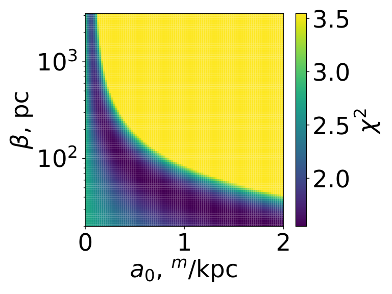
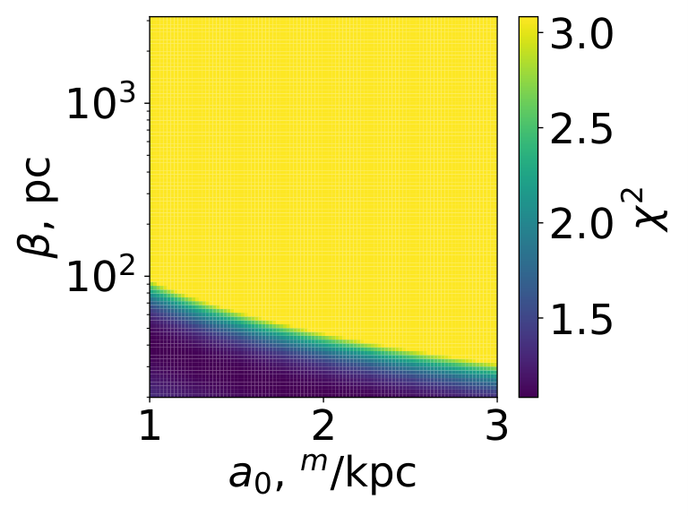
Independently from best-fit minimization we calculate $\chi^{2}$ values obtained from the formula (4) on $(a_{0},\beta)$ grid and find the minimum value of $\chi^{2}$ on the grid. Values $a_{0},\beta$ of the grid corresponding to the minimum $\chi^{2}$ value are considered the best approximation values. We also estimate the standard error values of the parameters $a_{0},\beta$ determination by $1\sigma$ -contour on $\chi^{2}$ map. Examples of $\chi^{2}(a_{0},\beta)$ solutions for some areas are illustrated in Fig. 3. Note that the shape of the blue area around the minimum value gives a representation about degeneration of the approximated parameters for a given area. Figures for all areas are placed in the Appendix B.

3.3 Comparison of two approaches and final values

Both approaches, described in Sections 3.1 and 3.2 were applied to all 40 areas. Values of the $a_{0}$ and $\beta$ parameters, obtained with both methods, are plotted in Fig. 4. Total Galactic extinction values ( $A_{Gal}$ ), calculated from $a_{0}$ and $\beta$ with Eq. (2) are plotted as well. For six areas no reasonable solution could be found with the described methods (these areas can be seen in Fig. 4 as outliers).

The values of $\chi^{2}$ were estimated for both methods. To compile the final list of the $a_{0}$ , $\beta$ parameters for our areas, we have taken values obtained with one of the two approaches (see Sections 3.1 and 3.2), which demonstrates the minimum $\chi^{2}$ . These data, including the Galactic extinction $A_{Gal}$ , calculated with Eq. (2), are presented in Table 1.

We have compared the calculated Galactic extinction with values, predicted by 2011ApJ…737..103S and 1998ApJ…500..525S (Fig. 5, values $A_{Gal}$ from 2011ApJ…737..103S and 1998ApJ…500..525S were obtained with Galactic extinction calculator https://irsa.ipac.caltech.edu/applications/DUST/). One can see that 1998ApJ…500..525S’s data better approximate our results than 2011ApJ…737..103S’s data. Our estimates of $A_{Gal}$ are on average 15% higher than those predicted in 1998ApJ…500..525S. The reason for the differences seems to be not high enough accuracy of the relations used in Eq.(3). In particular, this may be due to the fact that the coefficients $c_{1}$ and $c_{2}$ in Eq. (3) are not constants (see discussion in Section 2). This problem will be investigated by us later.

Table 1: Interstellar extinction in the selected areas

				This paper			SF2011 2011ApJ…737..103S
Area	l	b	N	$a_{0}$	$\beta$	$A_{Gal}$	$A_{Gal}$
1713	48.16	20.11	20	1.72 $\pm$ 0.273	84.365 $\pm$ 17.347	0.422 $\pm$ 0.11	0.3282 $\pm$ 0.0118
2482	36.21	20.11	43	1.554 $\pm$ 0.268	135.75 $\pm$ 31.224	0.613 $\pm$ 0.176	0.4183 $\pm$ 0.0124
3733	39.02	30.0	46	0.896 $\pm$ 0.081	150.371 $\pm$ 18.659	0.269 $\pm$ 0.041	0.2007 $\pm$ 0.0037
8789	22.15	30.0	33	1.108 $\pm$ 0.151	172.873 $\pm$ 34.206	0.383 $\pm$ 0.092	0.3483 $\pm$ 0.0189
17777	155.04	20.11	44	1.142 $\pm$ 0.087	107.93 $\pm$ 9.877	0.358 $\pm$ 0.043	0.212 $\pm$ 0.0028
28666	90.66	64.95	72	0.061 $\pm$ 0.071	681.292 $\pm$ 1571.163	0.046 $\pm$ 0.118	0.0346 $\pm$ 0.0019
29945	155.51	64.95	76	0.013 $\pm$ 0.013	1798.0 $\pm$ 6346.7	0.027 $\pm$ 0.098	0.0453 $\pm$ 0.0006
34455	229.92	19.79	43	0.392 $\pm$ 0.066	152.425 $\pm$ 41.533	0.176 $\pm$ 0.056	0.1075 $\pm$ 0.0022
35483	206.02	19.79	116	0.343 $\pm$ 0.081	125.893 $\pm$ 41.57	0.128 $\pm$ 0.052	0.0866 $\pm$ 0.0012
36249	228.87	30.0	112	0.113 $\pm$ 0.015	3904.2 $\pm$ 7294.1	0.883 $\pm$ 1.654	0.0945 $\pm$ 0.0022
64053	285.22	64.95	41	1.667 $\pm$ 1.0	23.263 $\pm$ 12.645	0.043 $\pm$ 0.035	0.0435 $\pm$ 0.0012
79217	20.04	20.11	21	14.081 $\pm$ 0.202	35.03 $\pm$ 0.0	1.435 $\pm$ 0.021	1.1739 $\pm$ 0.0229
82277	98.09	$-$ 30.0	73	1.242 $\pm$ 0.143	168.756 $\pm$ 29.785	0.419 $\pm$ 0.088	0.2886 $\pm$ 0.014
83604	94.92	$-$ 19.79	57	1.118 $\pm$ 0.167	90.967 $\pm$ 16.123	0.3 $\pm$ 0.07	0.2292 $\pm$ 0.005
84386	79.8	$-$ 20.11	56	6.589 $\pm$ 256.178	12.294 $\pm$ 480.196	0.236 $\pm$ 12.987	0.2119 $\pm$ 0.0022
84622	69.96	$-$ 20.11	49	0.586 $\pm$ 0.1	218.42 $\pm$ 56.704	0.372 $\pm$ 0.116	0.2664 $\pm$ 0.0034
96855	78.05	19.79	99	0.323 $\pm$ 0.04	210.001 $\pm$ 80.871	0.201 $\pm$ 0.081	0.1835 $\pm$ 0.0028
97942	83.32	30.0	45	0.727 $\pm$ 0.222	102.591 $\pm$ 35.665	0.149 $\pm$ 0.069	0.1325 $\pm$ 0.0059
98650	188.79	$-$ 30.0	36	1.463 $\pm$ 0.182	577.226 $\pm$ 250.491	1.689 $\pm$ 0.762	0.8784 $\pm$ 0.026
99901	185.98	$-$ 20.11	69	3.364 $\pm$ 0.235	130.833 $\pm$ 14.606	1.28 $\pm$ 0.169	0.9715 $\pm$ 0.0505
100961	164.88	$-$ 20.11	121	2.847 $\pm$ 0.787	45.192 $\pm$ 12.992	0.374 $\pm$ 0.149	0.3349 $\pm$ 0.0105
112048	194.06	19.79	224	0.144 $\pm$ 0.01	771.115 $\pm$ 183.167	0.329 $\pm$ 0.081	0.1187 $\pm$ 0.0028
112305	183.16	20.11	143	0.316 $\pm$ 0.02	248.257 $\pm$ 22.276	0.228 $\pm$ 0.025	0.1503 $\pm$ 0.0012
113239	168.05	19.79	93	1.16 $\pm$ 0.082	81.896 $\pm$ 7.634	0.281 $\pm$ 0.033	0.2066 $\pm$ 0.0031
114025	186.68	30.0	39	0.555 $\pm$ 0.152	149.965 $\pm$ 52.302	0.166 $\pm$ 0.074	0.1078 $\pm$ 0.0034
136719	75.25	$-$ 45.39	71	0.852 $\pm$ 0.178	244.611 $\pm$ 66.037	0.293 $\pm$ 0.1	0.1791 $\pm$ 0.0062
137487	63.15	$-$ 45.39	73	5.444 $\pm$ 0.636	30.045 $\pm$ 3.757	0.23 $\pm$ 0.039	0.1978 $\pm$ 0.0025
138857	62.93	$-$ 30.0	67	0.353 $\pm$ 0.094	168.121 $\pm$ 55.478	0.119 $\pm$ 0.05	0.1008 $\pm$ 0.0022
149151	143.06	$-$ 65.32	119	0.081 $\pm$ 0.121	332.83 $\pm$ 1571.163	0.03 $\pm$ 0.147	0.1015 $\pm$ 0.0019
151503	135.0	$-$ 45.39	55	0.955 $\pm$ 0.176	317.56 $\pm$ 100.983	0.426 $\pm$ 0.157	0.2597 $\pm$ 0.0245
152806	169.88	$-$ 44.99	47	1.526 $\pm$ 0.177	395.27 $\pm$ 62.142	0.853 $\pm$ 0.167	0.4179 $\pm$ 0.0105
160342	133.95	$-$ 30.0	228	0.722 $\pm$ 0.182	102.905 $\pm$ 28.656	0.149 $\pm$ 0.056	0.1045 $\pm$ 0.0053
161428	139.92	$-$ 19.79	125	0.711 $\pm$ 0.15	92.061 $\pm$ 22.274	0.193 $\pm$ 0.062	0.1235 $\pm$ 0.0047
162401	119.88	$-$ 20.11	104	0.983 $\pm$ 0.13	74.29 $\pm$ 12.014	0.212 $\pm$ 0.044	0.1647 $\pm$ 0.0019

4 Approximation for $a_{0},\beta$ parameters over the entire sky

Our final step is the approximation for $a_{0},\beta$ parameters over the entire sky by spherical harmonics (see Appendix A for details). Thirty four of the selected areas were used for the approximation, they are listed in Table 1 (N is number of stars in the area). The results are presented in Table 2, Eqs. (5)-(7) and Fig. 6.

These relationships will apparently apply better at higher extinction where the dust is averaged over a long line, and it will work less well at high latitudes. This should be checked when we extend our consideration to low latitudes and to (on average more distant) non-MS stars (see Section 5).

Table 2: The coefficients in the approximation of spherical harmonics

	$a_{0}$	$\beta$	$A_{Gal}$
$A_{00}$	6.484 $\pm$ 1.532	1151.305 $\pm$ 495.928	1.225 $\pm$ 0.239
$A_{10}$	$-$ 2.388 $\pm$ 1.677	578.567 $\pm$ 542.883	$-$ 0.279 $\pm$ 0.262
$A_{11}$	$-$ 7.645 $\pm$ 2.412	874.441 $\pm$ 780.663	$-$ 0.221 $\pm$ 0.377
$A_{20}$	$-$ 1.345 $\pm$ 1.640	516.379 $\pm$ 530.792	$-$ 0.470 $\pm$ 0.256
$A_{21}$	0.274 $\pm$ 2.099	554.834 $\pm$ 679.292	$-$ 0.570 $\pm$ 0.328
$A_{22}$	6.331 $\pm$ 2.271	$-$ 455.485 $\pm$ 735.097	0.793 $\pm$ 0.355

a_{0}=+6.484Y_{0}^{0}\left(l,\frac{\pi}{2}-b\right)-2.388Y_{1}^{0}\left(l,\frac{\pi}{2}-b\right)-7.645Y_{1}^{1}\left(l,\frac{\pi}{2}-b\right)-\\ -1.345Y_{2}^{0}\left(l,\frac{\pi}{2}-b\right)+0.274Y_{2}^{1}\left(l,\frac{\pi}{2}-b\right)+6.331Y_{2}^{2}\left(l,\frac{\pi}{2}-b\right)

(5)

\beta=+1151.305Y_{0}^{0}\left(l,\frac{\pi}{2}-b\right)+578.567Y_{1}^{0}\left(l,\frac{\pi}{2}-b\right)+874.441Y_{1}^{1}\left(l,\frac{\pi}{2}-b\right)+\\ +516.379Y_{2}^{0}\left(l,\frac{\pi}{2}-b\right)+554.834Y_{2}^{1}\left(l,\frac{\pi}{2}-b\right)-455.485Y_{2}^{2}\left(l,\frac{\pi}{2}-b\right)

(6)

A_{Gal}=+1.225Y_{0}^{0}\left(l,\frac{\pi}{2}-b\right)-0.279Y_{1}^{0}\left(l,\frac{\pi}{2}-b\right)-0.221Y_{1}^{1}\left(l,\frac{\pi}{2}-b\right)-\\ -0.470Y_{2}^{0}\left(l,\frac{\pi}{2}-b\right)-0.570Y_{2}^{1}\left(l,\frac{\pi}{2}-b\right)+0.793Y_{2}^{2}\left(l,\frac{\pi}{2}-b\right)

(7)

5 Future plans

This pilot study explores the possibility to construct an equation for quick estimation of interstellar extinction values. In our further work, we plan to include non-MS stars from LAMOST/Gaia and to extend our results to lower galactic latitudes.

Beside that, we plan to extend our procedure to the Southern sky, using RAVE survey ( $\sim$ 460,000 objects) 2017AJ….153…75K and upcoming 4MOST and MOONS surveys. 4MOST (2022+) 2019Msngr.175….3D, 4-metre Multi-Object Spectrograph Telescope is a second-generation instrument built for ESO’s 4.1-metre Visible and Infrared Survey Telescope for Astronomy (VISTA) at the Paranal Observatory (Chile). MOONS (2020+) 2016ASPC..507..109C, is the Multi-Object Optical and Near-infrared Spectrograph for the ESO VLT (8.2 m).

For the Northern sky, besides LAMOST, other spectroscopic surveys can be used. Among them are APOGEE ( $\sim$ 450,000 objects) 2018MNRAS.476.2117R, SEGUE ( $\sim$ 350,000 objects) 2009AJ….137.4377Y, and upcoming WEAVE (2021+) 2016sf2a.conf..271S, WHT Enhanced Area Velocity Explorer, a multi-object survey spectrograph for the 4.2-m William Herschel Telescope (WHT) at the Observatorio del Roque de los Muchachos (La Palma, Canary Islands).

6 Conclusions

Spectroscopic surveys can serve as exceptional sources not only of stellar parameter values but also of nature of interstellar dust and its distribution in the Milky Way. Stellar atmospheric parameters, when used with trigonometric parallaxes, provide us with an exceptional opportunity to estimate independently both the distance $d$ and interstellar extinction $A_{V}$ .

We have cross-identified objects in LAMOST DR5 spectroscopic survey and Gaia DR2/EDR3 surveys. For 40 test areas located at high galactic latitudes ( $\left|b\right|>20^{\circ}$ ) we have constructed $A_{V}(d)$ relations and approximated them by the cosecant law (1). We have determined then $a_{0}$ and $\beta$ values for each area and made a 2D approximation for the entire sky (except low galactic latitudes and the southern polar cap). We have also estimated the Galactic extinction for the test areas by spherical harmonics (Eqs. 5-7), and the comparison of our results with data from 2011ApJ…737..103S demonstrates a good agreement.

The Eqs. (5), (6) can be used for calculation of parameters $a_{0}$ and $\beta$ and, consequently, for estimation of interstellar extinction from (1). These results are valid for high Galactic latitudes ( $\left|b\right|>20^{\circ}$ ) and distances within about 6 to 8 kpc from the Sun. The Eq. (7) allows one to estimate the Galactic extinction for high Galactic latitudes.

Acknowledgements.

We are grateful to our reviewers whose constructive comments greatly helped us to improve the paper. We thank Alexei Sytov for valuable remarks and suggestions. The work was partly supported by NSFC/RFBR grant 20-52-53009. KG research was supported by the Russian Science Foundation (RScF) grant No. 17-72-20119. AN research has been supported by the Interdisciplinary Scientific and Educational School of Moscow University “Fundamental and Applied Space Research”. This research has made use of NASA’s Astrophysics Data System, and use of TOPCAT, an interactive graphical viewer and editor for tabular data 2005ASPC..347…29T.

Author Contributions: The authors made equal contribution to this work; O.M. wrote the paper.

References

(1) P. P. Parenago, Astron. Zh., 13, 3, 1940.
(2) G. de Vaucouleurs, A. de Vaucouleurs, and J. R. Corwin, Second reference catalogue of bright galaxies, 1976, 0, 1976.
(3) A. Sandage, Astrophys. J. , 178, 1, 1972.
(4) L. Spitzer, Physical processes in the interstellar medium (1978).
(5) P. P. Parenago, Popular Astronomy, 53, 441, 1945.
(6) A. S. Sharov, Astron. Zh. , 40, 900, 1963.
(7) A. K. Pandey and H. S. Mahra, Mon. Not. R. Astron. Soc. , 226, 635, 1987.
(8) D. J. Marshall, A. C. Robin, C. Reylé, M. Schultheis, and S. Picaud, Astron. Astrophys. , 453, 635, 2006.
(9) M. P. Fitzgerald, Astron. J. , 73, 983, 1968.
(10) T. Neckel and G. Klare, Astron. and Astrophys. Suppl. Ser. , 42, 251, 1980.
(11) F. Arenou, M. Grenon, and A. Gomez, Astron. Astrophys. , 258, 104, 1992.
(12) O. Malkov and E. Kilpio, Astrophys. Space. Sci. , 280, 115, 2002.
(13) E. Y. Kil’Pio and O. Y. Malkov, Astronomy Reports, 41, 10, 1997.
(14) P. B. Lucke, Astron. Astrophys. , 64, 367, 1978.
(15) R. Drimmel, A. Cabrera-Lavers, and M. López-Corredoira, Astron. Astrophys. , 409, 205, 2003.
(16) Planck Collaboration, A. Abergel, P. A. R. Ade, N. Aghanim, et al., Astron. Astrophys. , 571, A11, 2014.
(17) S. E. Sale, J. E. Drew, G. Barentsen, H. J. Farnhill, et al., Mon. Not. R. Astron. Soc. , 443, 2907, 2014.
(18) G. M. Green and et al, Astrophys. J. , 810, 25, 2015.
(19) R. Lallement, L. Capitanio, L. Ruiz-Dern, C. Danielski, et al., Astron. Astrophys. , 616, A132, 2018.
(20) G. M. Green, E. Schlafly, C. Zucker, J. S. Speagle, and D. Finkbeiner, Astrophys. J. , 887, 93, 2019.
(21) B. Q. Chen, Y. Huang, H. B. Yuan, C. Wang, et al., Mon. Not. R. Astron. Soc. , 483, 4277, 2019.
(22) D. J. Schlegel, D. P. Finkbeiner, and M. Davis, Astrophys. J. , 500, 525, 1998.
(23) E. F. Schlafly and D. P. Finkbeiner, Astrophys. J. , 737, 103, 2011.
(24) J. A. Cardelli, G. C. Clayton, and J. S. Mathis, Astrophys. J. , 345, 245, 1989.
(25) J. E. O’Donnell, Astrophys. J. , 437, 262, 1994.
(26) M. A. Fluks, B. Plez, P. S. The, D. de Winter, B. E. Westerlund, and H. C. Steenman, Astron. and Astrophys. Suppl. Ser. , 105, 311, 1994.
(27) K. A. Larson and D. C. B. Whittet, Astrophys. J. , 623, 897, 2005.
(28) E. L. Fitzpatrick and D. Massa, Astrophys. J. , 663, 320, 2007.
(29) K. D. Gordon, S. Cartledge, and G. C. Clayton, Astrophys. J. , 705, 1320, 2009.
(30) A. L. Luo, Y. H. Zhao, G. Zhao, and et al., VizieR Online Data Catalog, V/164, 2019.
(31) Gaia Collaboration, T. Prusti, J. H. J. de Bruijne, A. G. A. Brown, et al., Astron. Astrophys. , 595, A1, 2016.
(32) Gaia Collaboration, A. G. A. Brown, A. Vallenari, T. Prusti, et al., Astron. Astrophys. , 616, A1, 2018.
(33) Gaia Collaboration, A. G. A. Brown, A. Vallenari, T. Prusti, J. H. J. de Bruijne, C. Babusiaux, and M. Biermann, Gaia early data release 3: Summary of the contents and survey properties, 2020.
(34) G. Bono, G. Iannicola, V. F. Braga, I. Ferraro, et al., Astrophys. J. , 870, 115, 2019.
(35) C. Jordi, M. Gebran, J. M. Carrasco, J. de Bruijne, et al., Astron. Astrophys. , 523, A48, 2010.
(36) C. A. L. Bailer-Jones, J. Rybizki, M. Fouesneau, G. Mantelet, and R. Andrae, Astron. J. , 156, 58, 2018.
(37) D. W. Evans, M. Riello, F. De Angeli, J. M. Carrasco, et al., Astron. Astrophys. , 616, A4, 2018.
(38) C. Danielski, C. Babusiaux, L. Ruiz-Dern, P. Sartoretti, and F. Arenou, Astron. Astrophys. , 614, A19, 2018.
(39) Gaia Collaboration, C. Babusiaux, F. van Leeuwen, M. A. Barstow, et al., Astron. Astrophys. , 616, A10, 2018.
(40) C. A. L. Bailer-Jones, Mon. Not. R. Astron. Soc. , 411, 435, 2011.
(41) M. J. Pecaut and E. E. Mamajek, Astrophys. J. Suppl. Ser. , 208, 9, 2013.
(42) M. Newville, T. Stensitzki, D. B. Allen, and A. Ingargiola, LMFIT: Non-Linear Least-Square Minimization and Curve-Fitting for Python, 2014, URL https://doi.org/10.5281/zenodo.11813.
(43) R. Lallement, C. Babusiaux, J. L. Vergely, D. Katz, F. Arenou, B. Valette, C. Hottier, and L. Capitanio, Astron. Astrophys. , 625, A135, 2019.
(44) F. Anders, A. Khalatyan, C. Chiappini, A. B. Queiroz, et al., Astron. Astrophys. , 628, A94, 2019.
(45) A. Kunder and et al, Astron. J. , 153, 75, 2017.
(46) R. S. de Jong, O. Agertz, A. A. Berbel, J. Aird, et al., The Messenger, 175, 3, 2019.
(47) M. Cirasuolo and MOONS Consortium, in I. Skillen, M. Balcells, and S. Trager, eds., Multi-Object Spectroscopy in the Next Decade: Big Questions, Large Surveys, and Wide Fields, Astronomical Society of the Pacific Conference Series, volume 507, 109 (2016).
(48) I. Reis, D. Poznanski, D. Baron, G. Zasowski, and S. Shahaf, Mon. Not. R. Astron. Soc. , 476, 2117, 2018.
(49) B. Yanny and et al, Astron. J. , 137, 4377, 2009.
(50) D. J. B. Smith and et al, in C. Reylé, J. Richard, L. Cambrésy, M. Deleuil, E. Pécontal, L. Tresse, and I. Vauglin, eds., SF2A-2016: Proceedings of the Annual meeting of the French Society of Astronomy and Astrophysics, 271–280 (2016).
(51) M. B. Taylor, in P. Shopbell, M. Britton, and R. Ebert, eds., Astronomical Data Analysis Software and Systems XIV, Astronomical Society of the Pacific Conference Series, volume 347, 29 (2005).

Appendix A. Spherical harmonics

We use orthonormalized spherical harmonics $Y_{n}^{m}$ to calculate 2D approximation of extinction parameters. Only real parts of harmonics are used, hence we use harmonics of non-negative order $0\leq m\leq n$ . Therefore spherical harmonics are calculated by the following formulas:

Y_{0}^{0}(l,b)=\frac{1}{2}\sqrt{\frac{1}{\pi}},\hskip 11.74988ptY_{1}^{0}(l,b)=\frac{1}{2}\sqrt{\frac{3}{\pi}}\cos b,

Y_{1}^{1}(l,b)=\frac{1}{2}\sqrt{\frac{3}{\pi}}\cos l\sin b,\hskip 11.74988ptY_{2}^{0}(l,b)=\frac{1}{4}\sqrt{\frac{5}{\pi}}\left(3\cos^{2}b-1\right),

Y_{2}^{1}(l,b)=\frac{1}{2}\sqrt{\frac{15}{\pi}}\cos l\sin b\cos b,\hskip 11.74988ptY_{2}^{2}(l,b)=\frac{1}{4}\sqrt{\frac{15}{\pi}}\cos 2l\sin^{2}b.

Appendix B. Figures. Best-fit $\chi^{2}$ minimization and $\chi^{2}$ scan solutions for the areas used for determination of the interstellar extinction.

Figure 7: Best-fit for 1713, 2482, 3733.