Controller Synthesis for Omega-Regular and Steady-State SpecificationsConference: Proc. of the 21st International Conference on Autonomous Agents and Multiagent Systems (AAMAS 2022); May 9–13, 2022; Online670

The controller synthesis problem is often used to establish safety and performance guarantees of stochastic systems such as Markov decision processes (MDPs) by inducing Markov chains exhibiting some desirable behavior. The $\omega$-regular languages (Thomas90b; Perrin04) provide an expressive formalism to unambiguously express such safety and progress properties of MDPs, while Linear Temporal Logic (LTL) provides a convenient and interpretable way to encode such $\omega$-regular properties. For the verification or synthesis of systems subject to these properties, an $\omega$-regular objective is usually translated into a finite-state machine that monitors the traces of the MDP (deAlfa98). Successful executions cause the finite-state machine to take certain accepting transitions infinitely often, and ultimately avoid certain rejecting transitions. That is, $\omega$-regular objectives reason about the asymptotic trace behavior of an MDP. The related notion of asymptotic frequency of states visited is not accounted for in such objectives. To illustrate the utility of being able to reason about both of these types of behavior, consider a simple robot tasked to explore terrain on Mars. For such a mission, one may come up with $\omega$-regular specifications that its traces of behavior should satisfy. For example, we may impose that, whenever a state labeled “ice” is encountered, the robot must collect a sample and drop it off at a state labeled “base”. Furthermore, the robot may also need to spend a certain proportion of its time – but not too much time so as not to conflict with gathering ice samples – exploring certain regions of the Martian landscape. Indeed, the robot may be requested to spend at least 25% of its time in regions of interest, but no more than 50% of its time. This is easily encoded as a steady-state specification. Such specifications cannot be directly expressed in LTL.

LTL controller synthesis through probabilistic model checking approaches (deAlfa98; principlesOfModelChecking) generally begins by computing the product MDP from the original MDP and the finite-state machine representation of the given objective. Then, the union of accepting maximal end components (AMECs) are computed and a policy is found such that the agent reaches some such component. Once there, actions can be chosen arbitrarily such that all states within the AMEC are visited infinitely often, thereby ensuring that the acceptance condition of the automaton is met and the objective is therefore satisfied by said policy. Generally, this choice of actions within the AMECs is arbitrary. However, it is evident that these choices are critical in the situations with constraints on the steady-state distribution. This distribution characterizes the asymptotic frequency behavior of a Markov chain induced by some policy in an MDP.

The controller synthesis problem subject to steady-state specifications has been explored recently (SSC; ijcai2019-784; ijcai2020-563; atia2021steady) and the integration of LTL constraints has been considered for stochastic policy settings (kvretinsky2021ltl). In this paper, we seek to complement and unify much of the preceding work by reasoning about both $\omega$-regular properties as well as steady-state distributions simultaneously and without making common assumptions of ergodicity on the underlying MDP. The proposed approach finds an optimal expected-reward deterministic policy that satisfies given $\omega$-regular and steady-state specifications. The computation of deterministic policies is an important avenue of inquiry when guarantees or predictable behavior are desired (sarathy2021spotter).

We recall classical definitions and introduce notation for the paper.

For any state $s\in S$, we let $A(s)$ denote the set of actions that can be selected in state $s$. For states $s,s^{\prime}\in S$ and $a\in A(s)$, $T(s,a)(s^{\prime})$ equals $p(s^{\prime}|s,a)$. A run of $\mathcal{M}$ is a sequence $\langle s_{0},a_{1},s_{1},\ldots\rangle\in S\times(A\times S)^{*}$ such that $p(s_{i+1}|s_{i},a_{i+1})>0$ for all $i\geq 0$. A finite run is a finite such sequence. When convenient, runs are sometimes defined as sequences of states, without including actions. For a run $r=\langle s_{0},a_{1},s_{1},\ldots\rangle$, we define the corresponding labeled run as $L(r)=\langle L(s_{0}),L(s_{1}),\ldots\rangle\in\big(2^{AP}\big)^{+}$. A policy (or a strategy) is a recipe for a decision-maker to resolve the non-determinism of the LMDP. A policy in $\mathcal{M}$ is a function $\pi:S^{+}\to D(A)$ mapping finite runs to actions. A policy is finite-memory if it remembers a finite amount of information about the past and a finite-memory policy can be represented using a finite-state machine. In this paper, we are interested in finite-memory deterministic policies of the form $\pi:S\times Q\rightarrow A$, where $Q$ is a set of memory modes. This memory is obtained from the finite-state machine representation of the given linear-time specification to be satisfied. We write $\pi(a|s,q)\in\{0,1\}$ for the probability of choosing action $a$ in the state $s$ when the memory mode is $q$. For the remainder of this paper, we assume finite-memory deterministic policies $\pi$. For an LMDP $\mathcal{M}=(S,\beta,A,T,R,AP,L)$, a finite-memory deterministic policy $\pi$ resolves its non-determinism and gives rise to a Labeled Markov Chain (LMC) $\mathcal{M}_{\pi}=(S_{\pi},\beta_{\pi},T_{\pi},R_{\pi},AP_{\pi},L_{\pi})$. Note that an LMC is an LMDP whose set of actions is a singleton and hence can be omitted. It is customary to represent the probabilistic transition function $T$ of the LMC as a matrix such that $T_{i,j}=T(s_{i})(s_{j})$. When other information is not pertinent, we write an LMC as $(S,T)$.

Given an LMDP $\mathcal{M}=(S,\beta,A,T,R,AP,L)$, we define its underlying directed graph $G_{\mathcal{M}}=(V,E)$, where $V=S$ and $E\subseteq S\times S$ is such that $(s,s^{\prime})\in E$ if $T(s,a)(s^{\prime})>0$ for some $a\in A(s)$. A sub-MDP of $\mathcal{M}$ is an LMDP $\mathcal{M}^{\prime}=(S^{\prime},\beta^{\prime},A^{\prime},T^{\prime},R^{\prime},AP^{\prime},L^{\prime})$, where $S^{\prime}\subseteq S$, $A^{\prime}\subseteq A$ is such that $A^{\prime}(s)\subseteq A(s)$ for every $s\in S^{\prime}$, and $\beta^{\prime}$, $T^{\prime}$, $R^{\prime}$ and $L^{\prime}$ are analogous to $\beta$, $T$, $R$, and $L$ when restricted to $S^{\prime}$ and $A^{\prime}$. An end component (deAlfa98) of an LMDP $\mathcal{M}$ is a sub-MDP $\mathcal{M}^{\prime}$ of $\mathcal{M}$ such that $G_{\mathcal{M}^{\prime}}$ is strongly connected. A bottom strongly connected component (BSCC) of an LMC is any of its maximal end components (MECs), where a MEC is an end component that is maximal under set inclusion.

A deterministic Rabin automaton (DRA) $\mathcal{A}$ is a tuple $(\Sigma,Q,q_{0},\delta,F)$, where $\Sigma$ is a finite alphabet, $Q$ is a finite set of states, $q_{0}\in Q$ is the initial state, $\delta:Q\times\Sigma\to Q$ is the transition function, and $F=\left\{(B_{i},G_{i})\in 2^{Q}\times 2^{Q}\right\}_{i\in[m]}$ is the Rabin acceptance condition. A run $r$ of a DRA $\mathcal{A}$ on $w\in\Sigma^{\omega}$ is an $\omega$-word $r_{0},w_{0},r_{1},w_{1},\ldots$ in $(Q\cup\Sigma)^{\omega}$ such that $r_{0}=q_{0}$ and, for $i>0$, $r_{i}=\delta(r_{i-1},w_{i-1})$. We write $\infi(r)\subseteq Q$ for the set of states that appear infinitely often in the run $r$. A run $r$ of a DRA $\mathcal{A}$ is accepting if there is some $(B,G)\in F$ such that $\infi(r)\cap B=\emptyset$ and $\infi(r)\cap G\neq\emptyset$. The language of $\mathcal{A}$ (or, accepted by $\mathcal{A}$) is the subset of words in $\Sigma^{\omega}$ that have accepting runs in $\mathcal{A}$. A language is $\omega$-regular iff it is accepted by a DRA (principlesOfModelChecking).

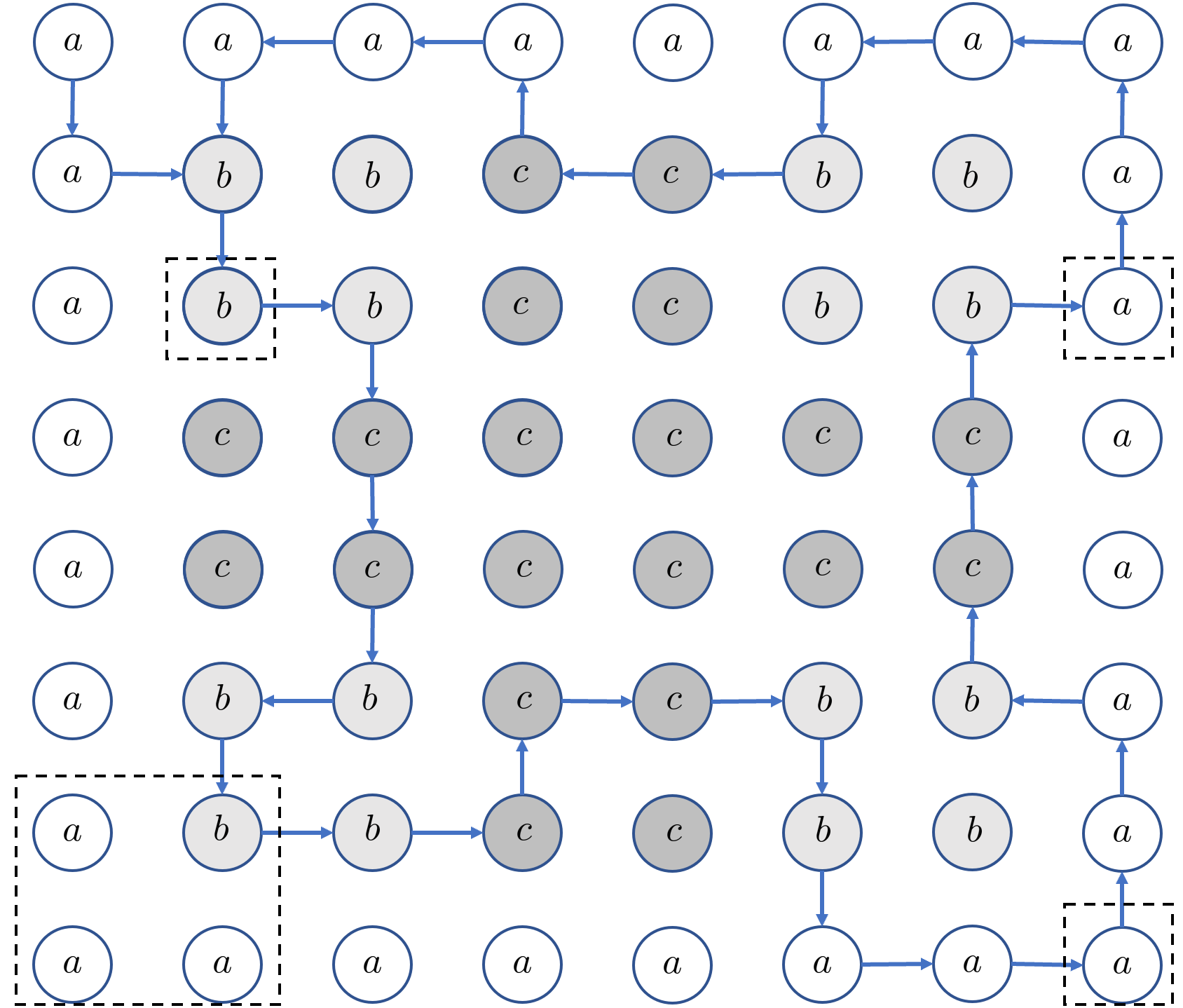
Given an LMDP $\mathcal{M}$ and an $\omega$-regular objective $\varphi$ given as a DRA $\mathcal{A}=(\Sigma,Q,q_{0},$ $\delta,F)$, the controller synthesis problem is to compute a policy that maximizes the probability of satisfaction of the $\omega$-regular objective. This problem is typically reduced to solving a product LMDP as shown in Figure 1. Given an LMDP $\mathcal{M}=(S,\beta,A,T,R,AP,L)$ and a DRA $\mathcal{A}=(2^{AP},Q,q_{0},\delta,F)$, their product LMDP $\mathcal{M}{\times}\mathcal{A}$ is the tuple $(S^{\times},\beta^{\times},A^{\times},T^{\times},R^{\times},Q,L^{\times})$, where $S^{\times}=S\times Q$; $\beta^{\times}\in D(S^{\times})$ is such that for all $(s,a)\in S^{\times}$, we have that $\beta^{\times}(s,q)$ equals $\beta(s)$ if $q=\delta(q_{0},L(s))$ and is $0$ otherwise; $A^{\times}=A$ and $A^{\times}(s,q)=A(s)$ for all $(s,q)\in S^{\times}$; $T^{\times}:S^{\times}{\times}A^{\times}\mapsto S^{\times}$ is such that for all $(s,q),(s^{\prime},q^{\prime})\in S^{\times}$ and $a\in A(s,q)$ we have $T^{\times}((s,q),a)(s^{\prime},q^{\prime})$ equals $T(s,a)(s^{\prime})$ if $q^{\prime}=\delta(q,L(s^{\prime}))$ and is $0$ otherwise; $R^{\times}((s,q),a)=R(s,a)$ for all $(s,q)\in S^{\times}$ and $a\in A(s,q)$; and $L^{\times}((s,q))=\left\{q\right\}$ for all $(s,q)\in S^{\times}$ (principlesOfModelChecking).

End components and runs are defined for products just like for LMDPs. The acceptance condition for the product LMDP can be lifted from the DRA and is used to define accepting MECs (AMECs). An AMEC of a product LMDP $\mathcal{M}\times\mathcal{A}$ is a MEC such that every run of the product LMDP that eventually dwells in it is accepting. Formally, a MEC $E=(S^{E},A^{E})$ of $\mathcal{M}\times\mathcal{A}$ is accepting if $S^{E}\cap(S\times B)=\emptyset$ and $S^{E}\cap(S\times G)\neq\emptyset$ for some $(B,G)\in F$. The satisfaction of an $\omega$-regular objective $\varphi$ by an LMDP $\mathcal{M}$ can be formulated in terms of AMECs of the product $\mathcal{M}\times\mathcal{A}_{\varphi}$, where $\mathcal{A}_{\varphi}$ is a DRA accepting $\varphi$. The maximum probability of satisfaction of $\varphi$ by $\mathcal{M}$ is the maximum probability, over all policies, that a run of the product LMDP $\mathcal{M}\times\mathcal{A}_{\varphi}$ eventually dwells in one of its AMECs (deAlfa98; maxProbs). Once an AMEC is reached, one must simply choose actions in the AMEC infinitely often in order to ensure that all states within it are visited infinitely often. It is worth noting that there always exists a stationary and deterministic policy over the product LMDP $\mathcal{M}\times\mathcal{A}$ to maximize the probability of visiting AMECs. This policy defines the optimal finite-memory policy over the original LMDP $\mathcal{M}$ to satisfy the $\omega$-regular objective given by the DRA $\mathcal{A}$. The DRA states $q\in Q$ in $\pi:S\times Q\rightarrow A$ in the product LMDP naturally define the memory mode of the finite-memory policy in the original LMDP (positionalToFinite).

A recurrent component $C\subseteq S$ of states is a nonempty set of states such that every state in $C$ communicates with every other state in $C$, and does not communicate with the states not in $C$. A unichain is an LMC that contains a single recurrent component and possibly some transient states. Otherwise, it is called a multichain. Our proposed approach finds a unichain LMC $\mathcal{M}_{\pi}$ in the original LMDP $\mathcal{M}$ that satisfies a given set of linear-time and steady-state constraints, though its corresponding product LMC $(\mathcal{M}\times\mathcal{A})_{\pi}$ in the product LMDP $\mathcal{M}\times\mathcal{A}$ may be a multichain.

The steady-state distribution $\text{Pr}^{\infty}\in D(S)$ of an LMC $\mathcal{M}=(S,\beta,T,R,AP,L)$ denotes the proportion of time spent in each state as the number of transitions within $\mathcal{M}$ approaches $\infty$. This distribution is characterized by the following system of steady-state equations:

The unichain condition is sufficient for LMCs to yield solutions to the steady-state equations in system (1). In particular, solutions in such settings yield the unique stationary distribution corresponding to the true steady-state behavior of the agent. For multichain LMCs, however, solutions to these equations may not be unique and may not correspond to the true steady-state behavior of the agent (norris1998markov). Indeed, consider the following simple example. Let $M$ be a Markov chain defined over states $S=\{s_{0},s_{1},s_{2}\}$ such that $T(s_{0})(s_{1})=0.6,T(s_{0})(s_{2})=0.4,T(s_{1})(s_{1})=T(s_{2})(s_{2})=1$. That is, state $s_{0}$ connects to $s_{1}$ and $s_{2}$ whereas these states self-loop with probability $1$. Solving the steady-state equations for this Markov chain yields the trivial identities $\text{Pr}^{\infty}(s_{0})=0,\text{Pr}^{\infty}(s_{1})=\text{Pr}^{\infty}(s_{1}),\text{Pr}^{\infty}(s_{2})=\text{Pr}^{\infty}(s_{2})$, and the equation $\text{Pr}^{\infty}(s_{1})+\text{Pr}^{\infty}(s_{2})=1$. Note that there are an infinite number of solutions to this equation. This elucidates the challenge of reasoning about steady-state constraints in multichain settings. We circumvent these challenges by focusing our attention on multichain product LMCs whose BSCCs share some state of the original LMC. We show that this is a necessary and sufficient condition for the original LMC to be a unichain. Furthermore, this restricts the BSCCs of the product LMC to be identical to one another in that their transition matrices are the same (up to row ordering). This yields a one-to-one correspondence between the solutions to the steady-state equations in the product LMC and the solutions to the steady-state equations in the original LMC. Since the original LMC is a unichain, this implies that these solutions will reflect the true steady-state behavior of the agent.

Given an LMDP $\mathcal{M}=(S,\beta,A,T,R,AP,L)$, the inverse of the labeling function $L^{-1}:2^{AP}\rightarrow 2^{S}$ returns the states where a given set of atomic propositions holds. More generally, given a Boolean formula over atomic propositions $\psi\triangleq\textbf{true}\mid p\in AP\mid\psi_{1}\wedge\psi_{2}\mid\neg\psi$, the function $L^{-1}(\psi)\subseteq S$ returns the set of states where $\psi$ holds. We now formalize what a steady-state specification is.

The controller synthesis problem given $\omega$-regular objectives has been studied at length in the literature, particularly under the name of LTL controller synthesis (etessami2007multi; yannakakis2008multi; forejt2011automated). Traditionally, such problems are solved by efficiently computing the set of AMECs (Chatte11) and finding a policy that reaches these and visits an accepting state therein infinitely often. The problem of deriving a control policy which satisfies constraints on the steady-state distribution of the resulting agent has been studied more recently (SSC; ijcai2019-784; ijcai2020-563). However, the literature on solving expected-reward constrained MDPs has often studied similar problems given that the expected-reward objective leverages the steady-state distribution or occupation measures, which are analogous to the steady-state distribution over state-action pairs, in order to determine expected policy values (kallenberg1983linear; Puterman:1994; altman_total_cost_98; 4927531). However, the common assumption that all policies yield an irreducible Markov chain is adopted for these methods. Indeed, the stronger ergodic assumption is often made in average-reward reinforcement learning problems ((sutton2018reinforcement), Sections 10.3, 13.6).

While various extensions to LTL have introduced average (averageLTL), discounted (discountedLTL), mean-payoff (LTL-lim), and frequency (frequencyLTL) modalities to the logic, to the best of the authors’ knowledge, the two facets of asymptotic behavior given by the steady-state (SS) distribution and linear-time (LTL) behavior of the agent have not yet been incorporated for the deterministic controller synthesis problem. To reiterate one of the challenges in this SS+LTL controller synthesis, the choice of actions within AMECs is critical since it is the states within said AMECs that will contribute to the steady-state distribution of the Markov chain induced by the solution policy. All other states would be transient or not visited, yielding a steady-state probability measure of 0. While this challenge is not present in traditional controller synthesis problems, a restricted form of it is addressed in the problem of LTL controller synthesis subject to persistent surveillance costs (svorevnova2013optimal). The goal in these problems is to satisfy a given LTL formula, or some restricted logic fragment thereof, while minimizing the cost incurred between satisfactions of a given surveillance goal specified as the repeated observance of a goal state. Perhaps the work most relevant to the results established in this paper stems from (SSC) and (ijcai2019-784). In (SSC), the Steady-State Control (SSC) problem is introduced. This is then generalized as Steady-State Policy Synthesis (SSPS) in (ijcai2019-784). In particular, the SSC problem entails finding a policy whose induced Markov chain satisfies a given steady-state distribution. This problem assumes that the underlying MDP is ergodic in that every policy yields irreducible Markov chains. This ensures that steady-state distributions reflect the true asymptotic behavior of the Markov chain. This is a fairly common assumption as observed recently by Altman in (Altman2019_11) for average-reward or -cost problems in constrained MDPs. In (ijcai2019-784), the SSPS problem is posed as a generalization of SSC by allowing steady-state constraints to contain inequalities as well as probability intervals. The solution proposed therein does not assume ergodic MDPs and instead finds an irreducible Markov chain within an arbitrary MDP, if one exists, such that steady-state constraints are satisfied. However, that approach cannot handle transient states nor multichain MDPs. These issues were addressed recently in (ijcai2020-563) and (atia2021steady), wherein a solution to the steady-state planning problem is proposed for multichain MDPs by focusing on a restricted class of policies, such as imposing that all actions be taken with some probability by the solution policy or that the long-term play is restricted to the bottom strongly connected (BSCCs) of the MDP. Indeed, the general problem of finding policies that satisfy arbitrary steady-state constraints in multichain MDPs remains open. This warrants an important distinction in our setting. Even though the product MDP over which we define our solution may be multichain, our setting is restricted in that we search for a policy that induces a product Markov chain whose BSCCs are isomorphic to one another in that their graph structures are identical. As we demonstrate, this is a necessary and sufficient condition for the original Markov chain (in the original MDP) to be a unichain, thereby ensuring that the steady-state equations admit a solution corresponding to the steady-state behavior of the agent.

Our solution to what we call the SS+LTL controller synthesis problem unifies much of the foregoing by reasoning about both linear-time $\omega$-regular properties as well as steady-state distributions simultaneously. The proposed approach finds an optimal expected-reward control policy that is deterministic and satisfies the given steady-state (SS) and LTL specifications. We do not assume that the underlying MDP is ergodic nor communicating. Instead, our solution finds a unichain Markov chain satisfying the given specifications, if one exists. This complements the recent results in (kvretinsky2021ltl), where a stochastic history-dependent (possibly with unbounded memory) policy as in (krass) is computed for the LTL-constrained steady-state policy synthesis problem. It is worth noting that, from a complexity perspective, these are fundamentally different problems due to the distinction between stochastic and deterministic policies. Indeed, finding a stochastic policy for this problem is in the complexity class P as demonstrated by the polynomial-time solution proposed in (kvretinsky2021ltl). On the other hand, the problem of computing a deterministic policy in this setting is an NP-complete problem (ijcai2019-784). Therefore, a polynomial-time solution is not likely to exist.

We combine the linear-time and steady-state specifications and solve the corresponding controller synthesis problem. Given an LMC $\mathcal{M}$ and a steady-state specification $\textbf{SS}_{[l,u]}(\psi)$, we say $\mathcal{M}$ satisfies $\textbf{SS}_{[l,u]}(\psi)$, denoted by $\mathcal{M}\models\textbf{ SS}_{[l,u]}(\psi)$, iff $\Sigma_{s\in L^{-1}(\psi)}\text{Pr}^{\infty}(s)\in[l,u]$ per Definition 2.1. Given an LTL formula $\phi$ defined inductively over a set of atomic propositions $AP$, Boolean connectives, and temporal modalities next, until, eventually, always ($\mathbf{X}$, $\mathbf{U}$, $\mathbf{F}$, $\mathbf{G}$), the satisfaction semantics $\mathcal{M}\models\phi$ are defined in the standard way (principlesOfModelChecking). We are interested in the combination of these LTL and SS specifications, henceforth referred to as SS+LTL specifications denoted by $\theta=(\phi_{\text{LTL}},(\textbf{SS}_{[l_{i},u_{i}]}\psi_{i})_{i})$. We say that $\mathcal{M}$ satisfies $\theta$, denoted by $\mathcal{M}\models\theta$, if $\mathcal{M}\models\phi_{\text{LTL}}$ and $\mathcal{M}\models\textbf{SS}_{[l_{i},u_{i}]}\psi_{i}$ for all $i$.

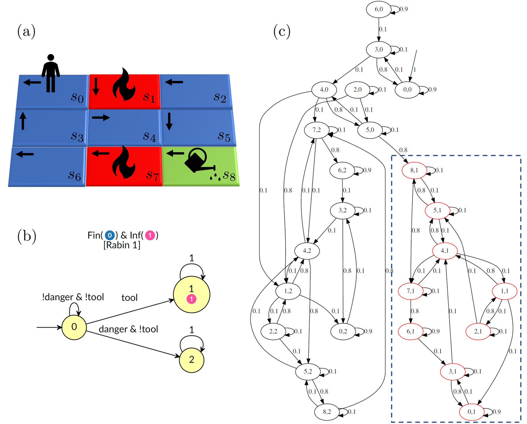
Let us fix an LMDP $\mathcal{M}=(S,\beta,A,T,R,AP,L)$ and an SS+LTL specification $\theta=(\phi_{\text{LTL}},(\textbf{SS}_{[l_{i},u_{i}]}\psi_{i})_{i})$ for the rest of the paper. Recall that the LTL formula $\phi_{\text{LTL}}$ can be compiled into a DRA $\mathcal{A}$. In what follows, we work with the product LMDP $\mathcal{M}\times\mathcal{A}=(S^{\times},\beta^{\times},A^{\times},T^{\times},R^{\times},Q,L^{\times})$, sometimes referred to as $\mathcal{M}^{\times}$ for convenience. Our goal is to characterize the existence of a stationary and deterministic policy $\pi:S\times Q\rightarrow A$ over the product LMDP. This, in turn, is equivalent to a finite-memory deterministic policy over the original LMDP. See Figure 2 for an example.

Let us first consider an agent whose goal is to find a stationary stochastic policy $\pi:S\times Q\rightarrow D(A)$ to maximize the expected reward in a product LMDP $\mathcal{M}\times\mathcal{A}$. If $\mathcal{M}\times\mathcal{A}$ is a unichain LMDP, the program in system (2) suffices to compute the optimal policy such that the solution yields the identity $x_{sqa}=\pi(a|s,q)\text{Pr}^{\infty}(s,q)=\pi(a|s,q)\sum_{a}x_{sqa}$ for $s\in S$, $q\in Q$, and $a\in A$ from which a stochastic policy can then be derived, where $x_{sqa}$ denotes the occupation measure of taking action $a$ in state $(s,q)\in S^{\times}$ (occupationMeasure).

Now, consider the more general case where the given product LMDP $\mathcal{M}\times\mathcal{A}$ may be multichain. Two key problems arise. First, the policy $\pi$ derived from the solution to (2) may not yield a unichain original LMC $\mathcal{M}_{\pi}$ (i.e., one with a single BSCC and possibly some transient states). Second, we note the challenges of deriving the correct steady-state distributions for an agent using linear programming in the multichain setting. In particular, in his seminal work (kallenberg1983linear), Kallenberg demonstrated that there is not a one-to-one correspondence between the steady-state distribution derived from linear programming solutions to expected-reward MDPs and the true steady-state distribution of the agent enacting the resulting policy when the Markov chain is multichain (i.e. contains multiple BSCCs, and possibly some transient states). On the other hand, unichains yield a one-to-one correspondence between the solution of the steady-state equations and the true steady-state behavior of the agent (Puterman:1994). Furthermore, the solution to these equations is unique in said setting. We thus focus on deriving an optimal solution policy $\pi:S\times Q\rightarrow A$ in a (potentially) multichain product LMDP $\mathcal{M}\times\mathcal{A}$ such that the induced original LMC $\mathcal{M}_{\pi}$ is a unichain and satisfies a given SS+LTL formula. The interplay with the product LMC $(\mathcal{M}\times\mathcal{A})_{\pi}$ introduces some challenges in deriving such a policy. In particular, it may be the case that the product LMC $(\mathcal{M}\times\mathcal{A})_{\pi}$ induced by the solution policy $\pi$ is multichain and its corresponding original LMC $\mathcal{M}_{\pi}$ is unichain. We present a novel solution which accounts for such settings by ensuring that all BSCCs in the product multichain $(\mathcal{M}\times\mathcal{A})_{\pi}$ share some state of the original LMC $\mathcal{M}_{\pi}$. This establishes that the original LMC $\mathcal{M}_{\pi}$ is a unichain. We further prove that the steady-state probabilities derived over such product LMCs yield a one-to-one correspondence with the true steady-state behavior of the agent in the original LMC.

First, let us consider the simpler case where the product LMC is a unichain. Note that the single BSCC may contain the same state $s\in S$ multiple times as $S^{\times}\ni(s,q),(s,q^{\prime}),\dots$ We will show that the partition $[s]=\{(s,q)\}_{q}$ naturally defined over the states of the product LMC to yield the states of the original LMC is such that $\text{Pr}^{\infty}(s)=\sum_{(s,q)\in[s]}\text{Pr}^{\infty}(s,q)$. That is, we can compute the steady-state probabilities over the product LMC and use these to derive those in the original LMC over which the SS+LTL specification is defined. This is enabled by the lumpability of the product LMC, defined below.

A partition over an LMC naturally defines another LMC, known as the aggregated LMC, where each state of the latter corresponds to one of the partition sets of the former. As we will show in Corollary 1, the original LMC is the aggregated LMC resulting from a lumpable partition of the product LMC.

Lemma 5.3, Theorem 5.4, and Corollary 5.5 establish the one-to-one correspondence between the steady-state probability derived for an irreducible product LMC and the steady-state distribution for the original LMC. Note that this result also holds for unichains since the steady-state probability measure of transient states therein would be zero. Now, let us consider the case where the product LMC is a multichain. We establish sufficient conditions for yielding the same one-to-one correspondence of steady-state distributions. Furthermore, we establish necessary and sufficient conditions for the multichain product LMC $(\mathcal{M}\times\mathcal{A})_{\pi}$ to yield a unichain original LMC $\mathcal{M}_{\pi}$.

To illustrate Theorem 5.4 and Lemmas 5.6 and 5.7, consider the multichain product LMC in Figure 4, where $T_{1}$ and $T_{2}$ denote the transition probability matrices for the two BSCCs. We will show that, because these two BSCCs are identical in terms of their transition matrices (rows may need to be reordered to reflect this), we have $\text{Pr}^{\infty}(s)=\sum_{(s,q)\in[s]}\text{Pr}^{\infty}(s,q)$ for states $s$ in the original LMC shown in Figure 4. The solution to the steady-state equations for this product LMC yields $\text{Pr}^{\infty}(s_{0},q_{0})=0,\text{Pr}^{\infty}(s_{1},\cdot)=1/6,\text{Pr}^{\infty}(s_{2},\cdot)=1/12$. The order of states in $T_{2}$ differs from that of $T_{1}$ in order to reflect that BSCCs can be identical up to row ordering. Note that the equivalence classes can be defined in terms of the isomorphic sets as $[s_{1}]=\langle s_{1}\rangle\bigcup\langle s^{\prime}_{1}\rangle$ and $[s_{2}]=\langle s_{2}\rangle\bigcup\langle s^{\prime}_{2}\rangle$.

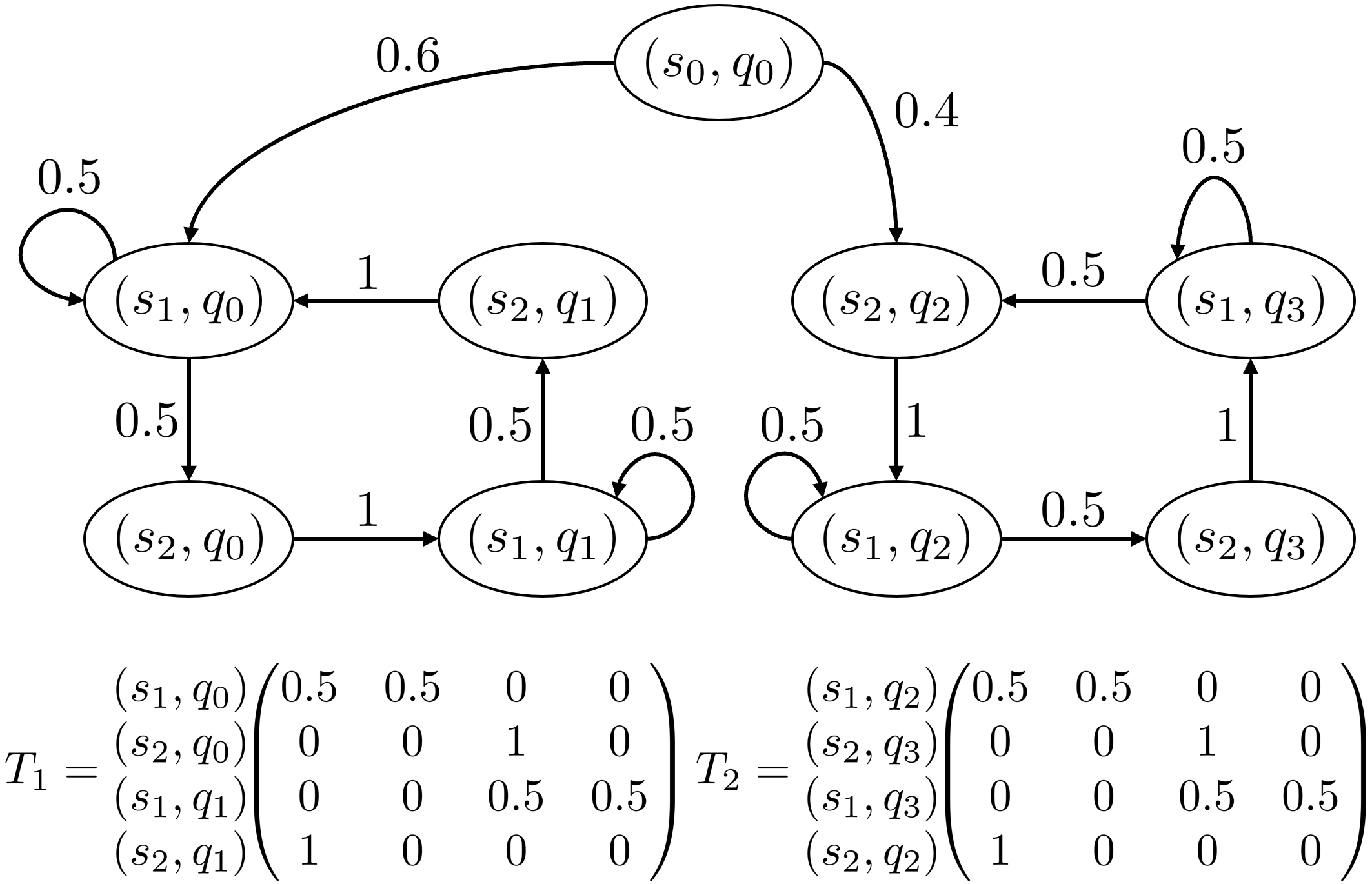
Now, consider the original LMC shown in Figure 4 corresponding to this product LMC. Solving the steady-state equations (1) for the original LMC yields $\text{Pr}^{\infty}(s_{0})=0,\text{Pr}^{\infty}(s_{1})=2/3,\text{Pr}^{\infty}(s_{2})=1/3$. Note that $\text{Pr}^{\infty}(s_{1})=\sum_{(s,q)\in[s_{1}]}\text{Pr}^{\infty}(s,q)$ and $\text{Pr}^{\infty}(s_{2})=\\ \sum_{(s,q)\in[s_{2}]}\text{Pr}^{\infty}(s,q)$ in accordance with Theorem 5.4 by leveraging the fact that $\text{Pr}^{\infty}(s,q)=\sum_{(s^{\prime},q^{\prime})\in\langle s\rangle}\text{Pr}^{\infty}(s^{\prime},q^{\prime})$ per Lemma 5.7.

Theorem 5.4 and Lemma 5.7 establish necessary and sufficient conditions for a multichain product LMC to yield a unichain original LMC in the original LMDP such that there is a one-to-one correspondence between the sum of steady-state probabilities $\sum_{q}\text{Pr}^{\infty}(s,q)$ in the former and the steady-state distribution $\text{Pr}^{\infty}(s)$ in the latter. Indeed, note that

holds when the product LMC is unichain or multichain given that the original LMC is unichain. This is the case when all BSCCs in the product LMC are identical as mentioned in Lemma 5.7, which is the case when all BSCCs in the product LMC share some state in $S$ per Lemma 5.6.

We can now add constraints to program (2) to ensure that the solution policy $\pi$ is deterministic and yields a unichain original LMC $\mathcal{M}_{\pi}$ in the original LMDP $\mathcal{M}$ even though the product LMC $(\mathcal{M}\times\mathcal{A})_{\pi}$ induced in the product LMDP $\mathcal{M}\times\mathcal{A}$ may be multichain. We begin with constraints to enforce a deterministic policy. Constraint $(iii)$ ensures that a positive occupation measure implies that the action corresponding to it is selected as part of the solution policy and $(iv)$ enforces a valid probability distribution, where $\pi(a|s,q)\in\{0,1\}$.

We can now add additional constraints that utilize the policy $\pi$ in constraints $(iii)$ and $(iv)$ in order to establish that some accepting state within an AMEC is reached by this policy and visited infinitely often. This would, in turn, satisfy the LTL specification $\phi_{\text{LTL}}$ of the given SS+LTL specification $\theta$. For simplicity, we assume an initial state $s_{0}$ in the underlying LMDP $\mathcal{M}$ (i.e. $\beta(s_{0})=1$). In order to ensure that there is a path from the initial state $(s_{0},\delta(q_{0},L(s_{0})))\in S^{\times}$ in the product LMDP $\mathcal{M}^{\times}$ to some recurrent component in the union of AMECs which contains nodes in $\bigcup_{i}G_{i}$ (i.e. nodes that are part of the DRA acceptance pairs), we will use flow transfer constraints. This notion of flow reflects the probability of transitioning between states given a policy. Constraint $(v)$ sets the flow capacities, where $f_{sqs^{\prime}q^{\prime}}$ denotes flow from $(s,q)\in S^{\times}$ to $(s^{\prime},q^{\prime})\in S^{\times}$. Constraint $(vi)$ ensures that, for every state (except the starting state), if there is incoming flow, then it is strictly greater than the outgoing flow. This is handled by the product of some small constant $\epsilon$ and an indicator variable $\mathcal{I}_{sq}\in\{0,1\}$ denoting whether flow is being transferred from state $(s,q)$ to some other state. If there is no incoming flow, then there is no outgoing flow and $\mathcal{I}_{sq}$ must necessarily be zero. Constraint $(vii)$ ensures that, if there is incoming flow into a state $(s,q)\in S^{\times}$, then $\mathcal{I}_{sq}=1$. Constraint $(viii)$ ensures that, whenever there is incoming flow, there must also be some arbitrary amount of outgoing flow. The choice of denominator 2 here is arbitrary.

Constraint $(ix)$ ensures that the steady-state probability of states with no incoming flow (as determined by $\mathcal{I}_{sq}$ in constraint $(vi)$) is 0. This makes it so that unreachable BSCCs in the product LMC $(\mathcal{M}\times\mathcal{A})_{\pi}$ do not contribute to the steady-state distribution. Constraint $(x)$ encodes the steady-state specifications given by operators SS in $\theta$ and constraint $(xi)$ ensures that some state in the acceptance sets $\bigcup_{i}G_{i}$ of $\mathcal{A}$ is visited infinitely often to satisfy the LTL specification.

Recall that constraints $(i)$ and $(ii)$ yield the correct steady-state distribution if there is a single BSCC (per the unichain condition) or if all BSCCs in the product LMC $(\mathcal{M}\times\mathcal{A})_{\pi}$ are identical and the induced original LMC $\mathcal{M}_{\pi}$ is a unichain (per Lemma 5.7). This is the case when all BSCCs of $(\mathcal{M}\times\mathcal{A})_{\pi}$ share some state in $s\in S$ per Lemma 5.6. We must therefore ensure that, in the product LMC, some state in $S$ is shared (This is trivially true if there is only one BSCC). The one-to-one correspondence of paths between the original LMC and the product LMC will then guarantee that the former is unichain even if the latter is multichain. To accomplish this, we define three indicator variables $\mathcal{I}_{s},\mathcal{I}^{k},\mathcal{I}^{k}_{s}\in\{0,1\}$ whose value is 1 iff $(s,\cdot)$ shows up in some BSCC of the product LMC, the $k^{\text{th}}$ AMEC of the product LMDP has some state with positive steady-state probability (meaning that the AMEC, or a subset of it, will show up as a BSCC in the product LMC), and $(s,\cdot)$ has positive steady-state probability in the $k^{\text{th}}$ AMEC, respectively.

Let $AMEC$ denote the set of all AMECs in the product LMDP $\mathcal{M}\times\mathcal{A}$ and let $AMEC_{k}$ denote the $k^{\text{th}}$ AMEC. Constraint $(xii)$ ensures that $\mathcal{I}^{k}$ is 1 if some state in the $k^{\text{th}}$ AMEC has positive steady-state probability. Constraints $(xiii)$ and $(xiv)$ ensure that, for a given state $s\in S$ and the $k^{\text{th}}$ AMEC, some indicator variable $\mathcal{I}_{sq}$ is 1 for $(s,q)$ in the $k^{\text{th}}$ AMEC if and only if $\mathcal{I}^{k}_{s}=1$. Constraint $(xv)$ ensures that, if $\mathcal{I}_{s}$ is 1, then $(s,\cdot)$ shows up in every BSCC of the product LMC $(\mathcal{M}\times\mathcal{A})_{\pi}$, thereby enforcing that all BSCCs in $(\mathcal{M}\times\mathcal{A})_{\pi}$ are identical. Per Lemma 5.6, this ensures that the original LMC $\mathcal{M}_{\pi}$ is a unichain. Note that the sum $\sum_{k}(\mathcal{I}^{k}_{s}-\mathcal{I}^{k})$ is always non-positive and dividing by the number of AMECs bounds this result to be within $[-1,0]$. Finally, constraint $(xvi)$ ensures that some such shared state exists across all BSCCs of the product LMC.