Probing heavy charged fermions at $e^{+}e^{-}$ collider using the Optimal Observable Technique

Subhaditya Bhattacharya Affiliation: Department of Physics, Indian Institute of Technology Guwahati, Assam 781039, India Email: subhab@iitg.ac.in Sahabub Jahedi Affiliation: Department of Physics, Indian Institute of Technology Guwahati, Assam 781039, India Email: sahabub@iitg.ac.in Jose Wudka Affiliation: Department of Physics and Astrophysics, University of California, Riverside, USA Email: jose.wudka@ucr.edu

Abstract

In this work we study the production of color-neutral and singly-charged heavy leptons at the proposed International Linear Collider. We use the optimal observable technique to determine the statistical accuracy to which the coupling of such fermions to the $Z$ gauge boson (vector, axial or chiral) can be measured. We also consider a UV-complete model that contains these particles as well as a dark matter candidate, and consider some observable effects involving both; the correspondence to chargino production in supersymmetric models with heavy sleptons is briefly discussed.

Keywords

Beyond Standard Model,

e^{+}e^{-}

Experiments, Particle and resonance production

1 Introduction

The expected presence of physics beyond the Standard Model (BSM) is motivated by the observation of non-vanishing neutrino masses, the overwhelming evidence for dark matter (DM), and the need for an effective mechanism to explain the baryon asymmetry; in addition, theoretical issues such as the stabilization of Higgs vacuum, also point towards the presence of new physics (NP). The search for such new particles and interactions is one of the central programs at the Large Hadron Collider (LHC). Despite this effort, and excepting the discovery of the long sought-after Higgs boson in 2012 Aad:2012tfa; Chatrchyan:2012ufa, no direct observation of new physics at the LHC (or other experiments) has been confirmed, though there are significant hints Lees:2012xj; Aaij:2017tyk; Lees:2013uzd; Aaij:2017deq; Aaij:2021vac; Bennett:2002jb; Bennett:2006fi; Aoyama:2012wk; Aoyama:2020ynm; Abi:2021gix.

One major challenge facing the search for NP at the LHC is its large QCD background that makes the detection of possible weakly-coupled BSM physics difficult. Yet this type of NP is expected in several scenarios (e.g. many DM and neutrino mass generation paradigms), which makes the prospect of an electron-positron ( $e^{+}e^{-}$ ) collider, such as the International Linear Collider (ILC) Behnke:2013xla, a very attractive possibility for probing a variety of BSM physics. It is the goal of this paper to study some of the capabilities of the ILC and determine its sensitivity to simple NP extensions of the SM: we consider first the sensitivity of the ILC to an additional heavy vector-like fermion, and then to a SM extension that includes, in addition, a viable DM candidate. The discussion here presented can be easily extended to other proposed $e^{+}e^{-}$ colliders and to a diversity of other types of hypothesized BSM physics.

The current bounds on heavy lepton masses depend on their nature (chiral or vector-like) and dominating decay channels. For example, LEP put a bound on the mass of $101.2\,\hbox{GeV}$ (95% CL) on the mass of heavy, unstable, singly-charged fermion Achard:2001qw when its main decay channel is $\nu W^{\pm}$ , while the bound is $102.6\,\hbox{GeV}$ (95% CL) if it is stable Tanabashi:2018oca. Searches at LHC have been so far in three main directions: (i) triplet leptons associated with type III seesaw mechanism for neutrino mass generation Sirunyan:2017qkz; (ii) stable or long-lived charged leptons; and (iii) superpartners of the SM gauge bosons (neutralino and chargino). In the first case, CMS has put a ( $3\sigma$ ) bound of $840\,\hbox{GeV}$ Sirunyan:2017qkz (using $137\,\text{fb}^{-1}$ of data at $\sqrt{s}=13\,\hbox{TeV}$ ). The current bound for a long-lived singly charged fermion is $\sim$ 574 GeV Chatrchyan:2013oca (CMS, using $18.8\,\text{fb}^{-1}$ of data at $\sqrt{s}=8\,\hbox{TeV}$ ). The limit on chargino mass in supersymmetric theories from production of chargino pairs Aad:2019vnb is $\sim 400\,\hbox{GeV}$ when the neutralino mass is zero, and $\sim 250\,\hbox{GeV}$ from chargino-neutralino pair production Aad:2019qnd (both obtained at $13\,\hbox{TeV}$ CM energy).

In our discussion below we will first study the detectability of a singly-charged lepton with mass of either $150\,\hbox{GeV}$ or $245\,\hbox{GeV}$ at the ILC, with a center-of-mass (CM) energy of $500\,\hbox{GeV}$ and determine the optimal statistical precision to which its couplings to the $Z$ boson can be measured using the optimal-observable technique (OOT) Atwood:1991ka; Davier:1992nw; Diehl:1993br; Gunion:1996vv. Charged fermion pair production in the context of type-III seesaw framework has been studied in literature Das:2020gnt; Das:2020uer, but no study has been done yet using the optimal observable approach. We will then consider this particle in the context of a specific NP model and provide an event-level collider simulation of its dominating decay channel; this model has the added feature of containing a viable dark matter candidate, some of whose effects at the ILC will also be considered. We will discuss the effects of beam polarization and the extent to which the conclusions drawn for these specific cases can be generalized.

The OOT has been used previous in a variety of studies, including the estimation of the uncertainty of the Higgs couplings Gunion:1996vv; Hagiwara:2000tk; Dutta:2008bh and top-quark couplings at $e^{+}e^{-}$ colliders Grzadkowski:1996pc; Grzadkowski:1997cj; Grzadkowski:1998bh; Grzadkowski:1999kx; Grzadkowski:2000nx, of the top-quark interactions in a $\gamma\gamma$ collider Grzadkowski:2003tf; Grzadkowski:2004iw; Grzadkowski:2005ye, of the CP properties of Higgs boson at a muon collider Hioki:2007jc, and of possible non-standard top-quark couplings at LHC Gunion:1998hm; Hioki:2012vn; Hioki:2014eca; other studies using this technique include estimating the sensitivity to NP effects in flavor physics Bhattacharya:2015ida; Calcuttawala:2017usw; Calcuttawala:2018wgo and NP searches in top-quark production at $e\gamma$ colliders Cao:2006pu.

Our paper is organized as follows: the OOT is described in section 2; the phenomenological model that we will use to study the $Z$ couplings of a heavy charged lepton is presented in 3; sections 3.1 and 3.2 discuss the relevant cross-section calculations and OOT for this model; the UV-complete model and associated collider signals are examined in section 4; with section 5 containing parting comments and conclusions.

2 Optimal uncertainties

This section contains a summary of several results concerning the statistical uncertainty of experimental observables. These results have appeared previously (see, e.g., Diehl:1993br); they are included here for convenience and to ensure uniformity of notation.

We consider models where the SM has been complemented by some type of new physics; the (theoretical) differential cross section for any given collider process involving the production of new particles can be written in the form

\mathcal{O}=\frac{d\sigma_{\tt theo}}{d\phi}=\sum_{i}c_{i}f_{i}(\phi)\,,

(1)

where $\phi$ denotes the appropriate phase-space coordinates and the coefficients $c_{i}$ , composed of (sums of products of) coupling and numerical constants, parametrize the process in terms of the linearly-independent functions $f_{i}$ . In the following, we will discuss 2 $\rightarrow$ 2 scattering process for which there is a single phase-space variable, that we take as the CM scattering angle; naturally, $\phi$ changes according to the process under consideration and experimental convenience. The separation of coefficients $c_{i}$ and functions $f_{i}$ is not unique – we will comment on this below.

The goal is now to determine the coefficients $c_{i}$ as accurately as possible. If one assumes a constant event rate together with the fact that an experiment occurs over a finite time, the event number follows a Poisson distribution, then the optimal covariance matrix becomes

V_{ij}=\frac{M_{ij}^{-1}\sigma_{T}}{N}=\frac{1}{{\mathfrak{L}}_{\tt int}}M_{ij}^{-1}\,,

(2)

with

M_{ij}=\int\frac{f_{i}(\phi)f_{j}(\phi)}{\mathcal{O}(\phi)}d\phi\,,

(3)

where $\sigma_{T}=\int\mathcal{O}(\phi)d\phi$ and N is total number of events ( $N=\sigma_{T}{\mathfrak{L}}_{\tt int}$ ). ${\mathfrak{L}}_{\tt int}$ denotes the integrated luminosity over this period. The detailed derivation of the covariance matrix as in Eq. (2) has been furnished in the Appendix A for the convenience of the readers. This can also be achieved by choosing a weighting function $w_{i}(\phi)$ such that $c_{i}=\int w_{i}(\phi)\mathcal{O}(\phi)d\phi$ Gunion:1996vv, where the expression of $w_{i}(\phi)$ is given by,

w_{i}(\phi)=\frac{\sum_{j}M_{ij}^{-1}f_{j}(\phi)}{\mathcal{O}(\phi)}.

(4)

$V$ can be used to estimate the width of the distribution of the $c_{i}$ as follows. We assume that these parameters have average (or ‘seed’) values $c_{i}^{0}$ and define ( $\epsilon$ is an efficiency factor discussed below)

\chi^{2}=\epsilon\sum_{\{i,j\}=1}^{n}\delta c_{i}\,\delta c_{j}\left(V_{0}^{-1}\right)_{ij},\qquad\delta c_{i}=c_{i}-c_{i}^{0},\qquad V_{0}=\left.V\right|_{c=c^{0}}\,;

(5)

In practice the optimal observable technique (OOT) consists in using this covariance matrix to determine statistical uncertainties and correlations between the coefficients $c_{i}$ .

Regarding $\chi^{2}$ as a random variable, one can determine the probability ${\sf p}_{n}(\ell)$ (often termed the confidence level, C.L.) for $\chi^{2}\leq\ell$ to occur. If the $c_{i}$ are normally distributed this is given by the usual $\chi^{2}$ distribution with $n$ degrees of freedom: ${\sf p}_{n}(\ell)=1-\Gamma(n/2,\ell/2)/\Gamma(n/2)$ . In particular, ${\sf p}_{2}(1)=39.3\%$ , and ${\sf p}_{3}(1)=19.8\%$ so that for $n=2,\,3$ the $\ell=1$ C.L. is relatively low; a $68\%$ C.L. requires $\ell=2.3$ for $n=2$ and $\ell=3.5$ for $n=3$ . In the discussion below we will be mainly concerned with the regions determined by $\chi^{2}\leq\ell$ for a given $\ell$ , referring to them as the $\sqrt{\ell}$ - $\sigma$ regions; this can be contrasted to the common usage of “1- $\sigma$ standard deviation” referred to $\chi^{2}=2.3$ for 2 parameter space and $\chi^{2}=3.5$ for 3 parameter space. An illustration on how the $1$ - $\sigma$ regions change when we use a given C.L. is discussed in Appendix D.

In the following we will consider the (electron-positron) collider production of new physics (NP) which in turn decays to SM states; symbolically, $e^{+}e^{-}\rightarrow$ NP $\rightarrow$ SM. We denote the ‘hard’ cross section for $e^{+}e^{-}\rightarrow$ NP production by $\sigma^{\tt NP}$ , and by $\sigma^{\tt FS}$ the final-state cross section $e^{+}e^{-}\rightarrow$ NP $\rightarrow$ SM, including all event selection cuts aimed at reducing and SM background and enhancing the NP contribution. The efficiency factor $\epsilon$ in Eq. (5) is then defined by the ratio

\epsilon=\frac{\sigma^{\tt FS}}{\sigma^{\tt NP}}~,

(6)

We would also like to note further that the statistical analysis done in section 3 is based on the NP signal process without including the effects of SM backgrounds, since this requires a specific model for a detailed characterization of the final state events (we return to this in section 4). However, the efficiency $\epsilon$ in Eq. (5) includes not only the branching ratio of NP $\rightarrow$ SM final state, but also the effects of event selection cuts that suppress the SM background contamination. The values of $\epsilon$ must be then estimated using a complete model of NP production and decay; in the next section we will assume $\epsilon=0.001$ and $0.005$ , justified by the analysis of the specific model of section 4. The use of $\epsilon$ to include these effects is, of course, an approximation; it is appropriate for the type of situations we consider: the resonant production of new particles which then decay into a SM final state. This approximation would not be appropriate in processes where on-shell NP particle is similar in mass and spin to that of a SM particle leading to same signal and providing large interference (for example, a new $Z^{{}^{\prime}}$ boson having similar mass to SM $Z$ boson), or when the new particle contribution to the signal is virtual or in narrow-width s-channel resonance. In all such cases the cross section in Eq. (1) receives also a SM contribution, and the corresponding OOT must be modified (cf. e.g. Diehl:1993br); we will return to this issue in a future publication. However, the procedure as adopted here, will be less conclusive, given a large irreducible SM background contribution and the estimation of $\epsilon$ will be limited in this case.

As noted earlier the choice of $c_{i}$ and $f_{i}$ is not unique; in practice one uses a separation that is convenient computationally and, if possible, has some physical motivation. The final results are independent of this choice in the sense that, if we use different functions and coefficients, $f_{i}=\sum u_{ij}\tilde{f}_{j}$ and $\tilde{c}_{i}=\sum u_{ji}c_{j}$ , where $u_{ij}$ is a constant invertible matrix, $\chi^{2}$ in Eq. (5) is invariant.

The covariance matrix $V$ depends on the physical process under consideration and on the experimental parameters such as collider energy and luminosity. Therefore the above expression can also be used to determine the (minimal) collider properties that are required to obtain a given desired statistical uncertainty.

The seed coefficients $c_{i}^{0}$ take different values depending on the type of new physics being considered. One can then take a different approach and regard Eq. (1) as a generic expansion of the cross section under consideration in a convenient basis of functions $f_{i}$ . If a model has parameters $p_{a}$ , then the $c_{i}=c_{i}(p_{a})$ and $\delta c_{i}=c_{i}(p_{a}^{0}+\delta p_{a})-c_{i}(p_{a}^{0})$ ; from which the statistical uncertainties and correlations of the $p_{a}$ can be readily extracted; an example of this procedure when is presented in the next section. The case where the $c_{i}$ are linear combinations of the $p_{a}$ is considered in appendix C. The number of parameters $p_{a}$ can be larger than the number of coefficients $c_{i}$ ; in which case the measurements under consideration provide a consistency test of the model.

3 Phenomenological framework

In this and the following sections we will use the OOT to determine the accuracy to which the parameters of a simple model of BSM physics can be measured at the projected International Linear Collider (ILC). The model we consider is a simple extension of the SM by the addition of a heavy charged fermion $\psi^{\pm}$ , that can be produced by $Z$ and photon exchange (Fig. 1). We will discuss the precision to which the OOT allows the determination of the $\psi$ couplings to the $Z$ at an $e^{+}e^{-}$ collider.

This type of heavy fermion appears in various extensions of SM; e.g. those containing a fermion isodoublet $\left(\psi^{0},\psi^{-}\right)$ with hypercharge $Y_{\psi}=-1$ ; we elaborate upon a possible model framework below (Sect. 4). Here we adopt a purely phenomenological approach, allowing $\psi^{\pm}$ to have general chiral couplings to the $Z$ boson¹¹ 1 We postpone any constraints coming from chiral anomalies to our discussion of a specific model.:

\psi^{+}\psi^{-}Z:-~\frac{ie_{0}}{s_{2\tt w}}\gamma^{\mu}\left(a+b\gamma^{5}\right)~,

(7)

(where $e_{0}=U(1)_{\tt em}$ coupling, and $s_{2\tt w}=\sin(2\theta_{\tt w})$ ; $\theta_{\tt w}$ is the weak-mixing angle) assuming for simplicity ²² 2 It is worth noting that in weakly-coupled theories modifications to the photon minimal coupling are generated at 1 or higher loops and are correspondingly suppressed. that it has the usual minimal coupling to the photon:

\psi^{+}\psi^{-}\gamma:-~ie_{0}\gamma^{\mu}\,.

(8)

The paramters $a,\,b$ correspond to the $p_{a}$ discussed briefly at the end of section 2.

Refer to caption — Figure 1: Production of heavy charged fermions ( $\psi^{+}\psi^{-}$ ) at $e^{-}e^{+}$ collision (ILC).

We will call any specific choice of $a,\,b$ a hypothesis and the corresponding parameters as seed parameters, of which we will consider the following:

•

$a=\pm 1$ , $b=0$ (pure vector coupling).
•

$a=0$ , $b=\pm 1$ (pure axial vector coupling).
•

$a=\pm 1$ , $b=\pm 1$ (chiral coupling).

We note that, for this simple model, $b\rightarrow-b$ under a parity transformation, so we need to consider only $b\geq 0$ .

Using the couplings in Eqs. (7) and (8), we can evaluate $d\sigma_{\tt theo}$ and, upon selection of the $f_{i}$ , extract the coefficients $c_{i}=c_{i}(a,b)$ ; the hypothesis $a=a^{0},\,b=b^{0}$ corresponds to assuming that these coefficients have seed values $c_{i}^{0}=c_{i}(a^{0},b^{0})$ (cf. comments at the end of sect. 2). We then use Eq. (2) to compute the covariance matrix $V$ and corresponding $\chi^{2}$ ; the regions $\chi^{2}<$ const. determine the optimal statistical uncertainties Gunion:1996vv; Calcuttawala:2017usw, and the accuracy to which different hypotheses can be differentiated.

For the calculations below we will assume the following collider parameters:

m_{\psi^{\pm}}=150\,\hbox{GeV}\,,~\text{or}~245\,\hbox{GeV}\\ \,,\qquad\sqrt{s}=500\,\hbox{GeV}\,;\quad{\mathfrak{L}}_{\tt int}=567\,\text{fb}^{-1}\,,

where $\sqrt{s}$ is the CM energy of the collider and integrated luminosity ${\mathfrak{L}}_{\tt int}$ , whose values were taken from the ILC design parameters Behnke:2013xla. The lower value of $m_{\psi^{\pm}}$ is chosen above the current collider limit of $O(100)\,\hbox{GeV}$ Tanabashi:2018oca (Sect. 1) ³³ 3 This limit is obtained using the $\psi^{\pm}\rightarrow W^{\pm}+$ neutral decay, which naturally occurs in the simplest models containing a $\psi^{\pm}$ ; see Sect. 4.; the higher value is chosen to be close to threshold.

Our analysis is carried out for an $e^{+}e^{-}$ linear collider because (i) it provides a much cleaner platform where QCD processes are suppressed, and so provides much better opportunity for the precision measurements we consider here; (ii) the expected availability of (partially) polarized beams allows a better probe of the new physics we are considering; and (iii) the construction of the covariance matrix and $\chi^{2}$ can be done analytically, avoiding insertion of the quark distribution functions that are unavoidable in a hadron collider.

3.1 The $\psi^{+}\psi^{-}$ production cross section at an $e^{+}e^{-}$ collider

The amplitude for the process $e^{+}e^{-}\rightarrow\psi^{+}\psi^{-}$ , which we denote by ${\cal M}(\lambda_{e^{-}},\,\lambda_{e^{+}},\,\lambda_{\psi},\,\lambda_{\bar{\psi}})$ (where $\lambda_{i}=\pm 1$ denotes the helicity of particle $i$ ), is easily calculated Vega:1995cc:

	$\displaystyle{\cal M}(\lambda_{e^{-}},\,-\lambda_{e^{-}},\,\lambda_{\psi},\,-\lambda_{\psi})$	$\displaystyle=-ee_{0}\left(\lambda_{e^{-}}\lambda_{\psi}+\cos\theta\right)\left[1+\xi\left(a+b\lambda_{\psi}\beta_{\psi}\right)\right]\,;\quad\xi=\xi_{1}+\lambda_{e^{-}}\xi_{2}\,,$
	$\displaystyle{\cal M}(\lambda_{e^{-}},\,-\lambda_{e^{-}},\,\lambda_{\psi},\,\lambda_{\psi})$	$\displaystyle=-ee_{0}\left(\frac{2m_{\psi^{\pm}}\lambda_{\psi}\sin\theta}{\sqrt{s}}\right)\left(1+\xi a\right)\,,$		(9)

where $e$ is the electron charge, $\sqrt{s}$ the CM energy, $\beta_{\psi}=\sqrt{1-4m_{\psi^{\pm}}^{2}/s}$ , and

\xi_{1}=\frac{C_{v}}{s_{2\tt w}^{2}(1-m_{\tt z}^{2}/s)}\,,\qquad\xi_{2}=\frac{C_{a}}{s_{2\tt w}^{2}(1-m_{\tt z}^{2}/s)}\,,

(10)

with $C_{v}=(4s_{\tt w}^{2}-1)/2,\,C_{a}=1/2$ , the vector and axial couplings of the electron to the $Z$ , respectively (and $s_{\tt w}=\sin\theta_{\tt w}$ ). If $\hat{\bf p}_{e^{-}}$ and $\hat{\bf p}_{\psi^{-}}$ are unit vectors parallel to the corresponding momenta, then the scattering angle $\theta$ is defined by $\cos\theta=\hat{\bf p}_{e^{-}}\cdot\hat{\bf p}_{\psi^{-}}$ .

Using Eq. (9), the cross-section when the $e^{\pm}$ beams have partial polarizations $P_{e^{\pm}}$ (with $-1\leq P_{e^{\pm}}\leq 1$ ) is given by

	$\displaystyle\frac{d\sigma(P_{e^{+}},\,P_{e^{-}})}{d\Omega}$	$\displaystyle=\frac{(1-P_{e^{-}})(1+P_{e^{+}})}{4}\left(\frac{d\sigma}{d\Omega}\right)_{\lambda_{e^{-}}=-1}+\frac{(1+P_{e^{-}})(1-P_{e^{+}})}{4}\left(\frac{d\sigma}{d\Omega}\right)_{\lambda_{e^{-}}=1}\,,$
		$\displaystyle=\sum c_{i}f_{i}\,,$		(11)

where we choose ⁴⁴ 4 It is straightforward to verify that these functions are linearly independent

\{f_{1},\,f_{2},\,f_{3}\}=\frac{\beta_{\psi}}{2s}\left\{(2-\beta_{\psi}^{2}),\,\beta_{\psi}\cos\theta,\,\beta_{\psi}^{2}\cos^{2}\theta\right\}\,,

(12)

and

$\displaystyle\frac{c_{1}}{\alpha\alpha_{0}}=$	$\displaystyle\frac{1-P_{e^{-}}P_{e^{+}}}{2}\bigg[1+2\xi_{1}a+(\xi_{1}^{2}+\xi_{2}^{2})\left(a^{2}+\frac{\beta_{\psi}^{2}}{2-\beta_{\psi}^{2}}b^{2}\right)-2P_{\tt eff}\bigg\{\xi_{2}a+\xi_{1}\xi_{2}a^{2}+\frac{\beta_{\psi}^{2}}{2-\beta_{\psi}^{2}}\xi_{1}\xi_{2}b^{2}\bigg\}\bigg];$
$\displaystyle\frac{c_{2}}{\alpha\alpha_{0}}=$	$\displaystyle\frac{1-P_{e^{-}}P_{e^{+}}}{2}\bigg[2\xi_{2}b+4\xi_{1}\xi_{2}ab-P_{\tt eff}\bigg\{2\xi_{1}b+(\xi_{1}^{2}+\xi_{2}^{2})ab\bigg\}\bigg];$
$\displaystyle\frac{c_{3}}{\alpha\alpha_{0}}=$	$\displaystyle\frac{1-P_{e^{-}}P_{e^{+}}}{2}\bigg[1+2\xi_{1}a+(\xi_{1}^{2}+\xi_{2}^{2})(a^{2}+b^{2})-2P_{\tt eff}\bigg\{\xi_{2}a+\xi_{1}\xi_{2}(a^{2}+b^{2})\bigg\}\bigg];$	(13)

We defined

P_{\tt eff}=\frac{P_{e^{-}}-P_{e^{+}}}{1-P_{e^{-}}P_{e^{+}}}.

(14)

and $\alpha_{0}=e_{0}^{2}/(4\pi)$ , while $\alpha=e^{2}/(4\pi)$ is the usual fine-structure constant. It is also useful to note that $d\sigma/d\Omega$ is invariant under $b\rightarrow-b$ and $\theta\rightarrow\pi-\theta$ , a consequence of the invariance of Eqs. (7) and (8) under CP.

The spin-averaged total and differential cross-sections (corresponding to $P_{e^{\pm}}=0$ ) for different seed values of $\{a,b\}$ are plotted in Fig. 2. It is worth noting that the total cross sections exhibit the same behavior for the values of $a$ and $b$ considered, especially at large $s$ ; this is due to a combination of two effects. First, since $s_{\tt w}^{2}\simeq 1/4$ , $\xi_{1}\sim 0$ ; second, for large $s$ , $\beta_{\psi}\simeq 1$ ; it follows that the average cross section $\sigma\propto 1+\xi_{2}^{2}(a^{2}+b^{2})$ , explicitly displaying its dependence on $a$ and $b$ . In contrast the unpolarized differential cross section depends on $c_{2}\simeq\xi_{2}b$ and will have a very different behavior depending on the values of $b$ . As expected from unitarity, the total cross section drops with increasing CM energy.

According to the design report Behnke:2013xla, the ILC will produce highly polarized electron beam and moderately polarized positron beam; we will choose $P_{e^{-}}=-0.8,\,P_{e^{+}}=+0.2$ when considering this option. Also, for polarized beams we have

	$\displaystyle a>0:$	$\displaystyle\quad\sigma\left(P_{e^{-}},\,P_{e^{+}}\right)\geq\sigma\left(P_{e^{\pm}}=0\right)\,,$
	$\displaystyle a<0:$	$\displaystyle\quad\sigma\left(P_{e^{-}},\,P_{e^{+}}\right)\leq\sigma\left(P_{e^{\pm}}=0\right)\,,$		(15)

whence it follows that polarization will enhance detectability. We illustrate these features in figures 3 where we plot the total cross section for various seed values of $a,b$ and choices of $P_{e^{\pm}}$ .

3.2 Optimal statistical analysis at $\sqrt{s}=500~\rm GeV$

We now apply the optimal observable method described in Sect. 2 to the case of $\psi^{\pm}$ production at the ILC, using the parameters of Eq. (3); the cases of $250\,\hbox{GeV}$ and $2\,\hbox{TeV}$ CM energy collider are briefly discussed in appendix B.

3.2.1 $\chi^{2}=1$ surfaces in the $a-b$ plane

As a first step, we use the above expressions to obtain the coefficients $c_{i}$ and functions $f_{i}$ ; for example, for unpolarized beams ( $P_{e^{\pm}}=0$ ) Eqs. (12) and (13) give:

\begin{array}[]{|c|l|l|}\hline\cr\vrule\lx@intercol\hfil\sqrt{s}=500\,\hbox{GeV}\,,\quad P_{e^{\pm}}=0\hfil\lx@intercol\vrule\lx@intercol\cr\hline\cr m_{\psi^{\pm}}\,(\hbox{GeV})&\qquad\qquad\qquad c_{i}/(\alpha\alpha_{0})&f_{i}\times 10^{-8}\,\hbox{GeV}^{2}\cr\hline\cr\hline\cr&i=1:~\frac{1}{2}(1-0.086a+0.522a^{2}+0.245b^{2})&i=1:~217.60\\ 150&i=2:~\frac{1}{2}(1.442b-0.124ab)&i=2:~128.00\cos\theta\\ &i=3:~\frac{1}{2}(1-0.086a+0.552(a^{2}+b^{2}))&i=3:~102.40\cos^{2}\theta\\ \hline\cr&i=1:~\frac{1}{2}(1-0.086a+0.522a^{2}+0.011b^{2})&i=1:~78.02\\ 245&i=2:~\frac{1}{2}(1.442b-0.124ab)&i=2:~7.92\cos\theta\\ &i=3:~\frac{1}{2}(1-0.086a+0.552(a^{2}+b^{2}))&i=3:~1.58\cos^{2}\theta.\\ \hline\cr\end{array}

(16)

Next, the optimal 1- $\sigma$ statistical uncertainties in the NP parameters $a,\,b$ are obtained from the $\chi^{2}\leq 1$ regions using Eqs. (2) and (5) for the parameters in Eq. (3). As illustrative examples we manifest the seed values listed at the beginning of this section, and take ⁵⁵ 5 It is clear from Eq. (5) that if $\chi^{2}$ is held fixed, the $\delta c$ will scale as $1/\sqrt{\epsilon}$ , but the dependence of $\delta a,\,\delta b$ on $\epsilon$ is more complicated, see Eq. (16); in the calculations below we use $\delta c=c(a^{0}+\delta a,\,b^{0}+\delta b)-c^{0}$ in Eq. (5); see also section 2. $\epsilon=0.001,\,0.005$ as reasonable estimates of the efficiency of signal identification (see Sect. 4.1 for a discussion); we consider both unpolarized ( $P_{e^{\pm}}=0$ ) and polarized ( $P_{e^{\pm}}=^{+20\%}_{-80\%}$ ) beams. The results are presented in figure 4 (for $a^{0}\geq 0$ ), figure 5 (for $a^{0}=-1$ ) and Table 1. These results illustrate the advantages that polarization provides in the determination of the couplings of these new particles.

From these results we can see that of the cases considered, the $a^{0}=0,\,b^{0}=\pm 1$ (pure axial coupling) hypothesis has the largest statistical errors and is therefore the most challenging. Also worth noting is that, while the magnitude of the total cross section strongly affects the statistical uncertainties, it is not the only factor; this is illustrated by considering the $a^{0}=-1$ case where the unpolarized cross section is larger than the polarized one (Fig. 3) but the uncertainties are larger (Fig. 5). We also note that 1 $\sigma$ regions for the lower mass ( $150$ GeV) are smaller than those for higher mass ( $245$ GeV), making the determination of the NP couplings for the latter case more difficult.

Seed parameters		$P_{e^{\pm}}=0$				$P_{e^{\pm}}=^{+20\%}_{-80\%}$
		$\epsilon=0.005$		$\epsilon=0.001$		$\epsilon=0.005$		$\epsilon=0.001$
model	$m_{\psi^{\pm}}$ (GeV)	$\pm\Delta a$	$\pm\Delta b$	$\pm\Delta a$	$\pm\Delta b$	$\pm\Delta a$	$\pm\Delta b$	$\pm\Delta a$	$\pm\Delta b$
$a=1$ $b=0$	150	$+0.04$	$+0.11$	$+0.08$	$+0.24$	$+0.02$	$+0.10$	$+0.05$	$+0.23$
	150	$-0.04$	$-0.11$	$-0.09$	$-0.24$	$+0.02$	$+0.10$	$-0.05$	$-0.23$
	245	$+0.07$	$+0.87$	$+0.15$	$+1.95$	$+0.04$	$+0.05$	$+0.09$	$+0.91$
	245	$-0.07$	$-0.87$	$-0.17$	$-1.95$	$+0.04$	$+0.05$	$-0.09$	$-0.91$
$a=1$ $b=\pm 1$	150	$+0.06$	$+0.10$	$+0.13$	$+0.23$	$+0.03$	$+0.11$	$+0.07$	$+0.25$
	150	$-0.06$	$-0.10$	$-0.18$	$-0.24$	$-0.03$	$-0.11$	$-0.08$	$-0.24$
	245	$+0.07$	$+0.87$	$+0.15$	$+1.96$	$+0.04$	$+0.86$	$+0.09$	$+1.93$
	245	$-0.07$	$-0.87$	$-0.21$	$-1.96$	$-0.04$	$-0.86$	$-0.10$	$-1.92$
$a=0$ $b=\pm 1$	150	$+0.35$	$+0.06$	$+0.51$	$+0.13$	$+0.04$	$+0.09$	$+0.07$	$+0.22$
	150	$-0.27$	$-0.11$	$-0.41$	$-0.22$	$-0.05$	$-0.09$	$-0.11$	$-0.22$
	245	$+0.43$	$+0.66$	$+0.59$	$+1.39$	$+0.04$	$+0.66$	$+0.10$	$+1.50$
	245	$-0.26$	$-0.67$	$-0.13$	$-1.51$	$-0.04$	$-0.66$	$-0.11$	$-1.47$
$a=-1$ $b=0$	150	$+0.04$	$+0.09$	$+0.07$	$+0.21$	$+0.06$	$+0.06$	$+0.12$	$-0.16$
	150	$-0.04$	$-0.09$	$-0.07$	$-0.21$	$-0.08$	$-0.06$	$-0.63$	$-0.16$
	245	$+0.06$	$+0.76$	$+0.15$	$+1.75$	$+0.10$	$+0.48$	$+0.20$	$+1.23$
	245	$-0.06$	$-0.76$	$-0.15$	$-1.75$	$-0.21$	$-0.48$	$-0.71$	$-1.23$
$a=-1$ $b=\pm 1$	150	$+0.06$	$+0.10$	$+0.15$	$+0.22$	$+0.17$	$+0.11$	$+0.26$	$+0.14$
	150	$-0.05$	$-0.10$	$-0.11$	$-0.22$	$-0.34$	$-0.11$	$-0.48$	$-0.22$
	245	$+0.07$	$+0.78$	$+0.17$	$+1.79$	$+0.11$	$+0.71$	$+0.20$	$+1.31$
	245	$-0.06$	$-0.78$	$-0.14$	$-1.74$	$-0.60$	$-0.49$	$-0.70$	$-1.11$

Table 1: Optimal 1

\sigma

statistical uncertainty in the

a,b

couplings for both unpolarized and polarized (

P_{e^{\pm}}=^{+20\%}_{-80\%}

) beams and two values of

\epsilon

; we used the parameters in Eq. (3).

3.2.2 Differentiation of models

One of the most important uses of the OOT is the ability to estimate the extent to which different hypotheses can be distinguished. Specifically, we consider a “base” hypothesis $a=a^{0},\,b=b^{0}$ and, using Eq. (2), define

\left[\Delta\sigma(a^{0},b^{0};\,\bar{a},\bar{b})\right]^{2}=\epsilon\sum_{i,j}\left(c^{0}_{i}-\bar{c}_{i}\right)\left(c^{0}_{j}-\bar{c}_{j}\right)\left(V^{-1}_{0}\right)_{ij}\,,\quad V_{0}=V(c=c^{0})\,;

(17)

(where $c^{0}_{i}=c_{i}(a^{0},\,b^{0}),\,\bar{c}_{i}=c_{i}(\bar{a},\,\bar{b})$ ) which we take as a measure of the degree to which the $a=\bar{a},\,b=\bar{b}$ hypothesis can be distinguished from the base hypothesis; we refer to $\Delta\sigma$ as the statistical significance of the $\bar{a},\,\bar{b}$ hypothesis (which depends on the base model chosen).

We will use $\Delta\sigma$ as a measure of the separation of an alternate model from the base one. The distribution of $\Delta\sigma$ can also be used to determine the probability that $\Delta\sigma\leq\ell$ occurs; in general this distribution is not simple, but for the cases where $c_{0}$ and $\bar{c}$ have normal distributions with averages ${\mathbbm{c}}_{0},\,\bar{\mathbbm{c}}$ , and covariance matrices $V_{0}$ and $\bar{V}$ that are approximately proportional to the unit matrix, $\sigma_{0}^{2}{\mathbbm{1}},\,\bar{\sigma}^{2}{\mathbbm{1}}$ respectively, then $\sqrt{\Delta\sigma}$ is approximately normally distributed with average $|{\mathbbm{c}}_{0}-\bar{\mathbbm{c}}|/\sigma_{0}$ and variance $1+(\bar{\sigma}/\sigma_{0})^{2}$ ; in practice this means that the values quoted for $\Delta\sigma$ will have errors $\sim\pm\sqrt{1+(\bar{\sigma}/\sigma_{0})^{2}}$ . Similar results hold when $\Delta\sigma$ is written in terms of $a$ and $b$ provided they also are normally distributed.

We now consider a few examples⁶⁶ 6 For these choices $V_{0},\,\bar{V}$ are approximately proportional to ${\mathbbm{1}}$ . corresponding to some of the cases presented in Table 2 or in Figs. 6, 7, 8. If $a^{0}=1,\,b^{0}=1$ and $\bar{a}=-1,\,\bar{b}=0$ , and we choose $m_{\psi}=150\,\hbox{GeV}$ , unpolarized beams, $\epsilon=0.005$ , and ${\mathfrak{L}}_{\tt int}=567\,\text{fb}^{-1}$ , we find $\Delta\sigma\simeq 9$ with a $\pm 1.43$ uncertainty. Assuming now $m_{\psi}=245\,\hbox{GeV}$ , polarized beam ( $P_{e^{\pm}}=^{+20\%}_{-80\%}$ ), $\epsilon=0.001$ , and ${\mathfrak{L}}_{\tt int}=567\,\text{fb}^{-1}$ and taking $a^{0}=0,\,b^{0}=0$ as the base model, we find that when $\bar{a}=1,\,\bar{b}=0$ (the purely vector-like case) $\Delta\sigma=13.96$ with $\pm 1.05$ uncertainty; w if $\bar{a}=1,\,\bar{b}=1$ we find $\Delta\sigma=14.09$ with an uncertainty of $\pm 1.07$ . We do not consider the $a^{0}=0,b^{0}=\pm 1$ cases since the $\Delta\sigma$ distribution is not normal, and a full analysis statistical analysis of the $\Delta\sigma$ statistics lies beyond the scope of this paper; however, we expect that the uncertainties in these cases will continue to be $O(\lesssim 10\%)$ .

It is worth noting that, as expected, larger efficiency $\epsilon$ and luminosity ${\mathfrak{L}}_{\tt int}$ increases the significance, while larger masses reduce it. It is also important to note that though the significance $\Delta\sigma$ depends on the magnitude of the cross section of the base model, this is not the only factor. For the example considered, the unpolarized cross section of the base model $a^{0}=b^{0}=0$ is smaller than the one for polarized beams by about 30%, yet the significance of the $\bar{a}=0,\,|\bar{b}|=1$ models is the same, while that of $\bar{a}=1,\,\bar{b}=0$ is larger than expected from the cross-section alone.

\begin{array}[]{| c | c | c | c | c | c | c | c | c | c| c|}\hline\cr\vrule\hfil\hfil\lx@intercol\vrule\lx@intercol&\vrule\hfil\hfil\lx@intercol\vrule\lx@intercol&\vrule\hfil\hfil\lx@intercol\vrule\lx@intercol&\vrule\lx@intercol\hfil\text{significance($\Delta\sigma$)\,}\hfil\lx@intercol\vrule\lx@intercol\\ \cline{4-7}\cr\vrule\lx@intercol\hfil\text{model}\hfil\lx@intercol\vrule\lx@intercol&\vrule\lx@intercol\hfil\epsilon\hfil\lx@intercol\vrule\lx@intercol&\vrule\lx@intercol\hfil{\cal L}_{\tt int}~[\text{fb}^{-1}]\hfil\lx@intercol\vrule\lx@intercol&\vrule\lx@intercol\hfil\text{$m_{\psi^{\pm}}=150$ GeV}\hfil\lx@intercol\vrule\lx@intercol&\vrule\lx@intercol\hfil\text{$m_{\psi^{\pm}}=245$ GeV}\hfil\lx@intercol\vrule\lx@intercol\\ \cline{4-7}\cr&&&P_{e^{\pm}}=0&P_{e^{\pm}}=^{+20\%}_{-80\%}&P_{e^{\pm}}=0&P_{e^{\pm}}=^{+20\%}_{-80\%}\\ \hline\cr\hbox{\multirowsetup\begin{tabular}[]{l}$\bar{a}=1$\\ $\bar{b}=0$\end{tabular}}&0.001&567&6.13&25.03&3.42&13.96\\ &0.001&2000&11.51&47.03&6.62&26.22\\ &0.005&567&13.72&55.98&7.65&31.21\\ \hline\cr\hbox{\multirowsetup\begin{tabular}[]{l}$\bar{a}=1$\\ $\bar{b}=\pm 1$\end{tabular}}&0.001&567&11.46&29.81&3.58&14.09\\ &0.001&2000&21.52&56.00&6.73&26.46\\ &0.005&567&25.62&66.67&8.01&31.50\\ \hline\cr\hbox{\multirowsetup\begin{tabular}[]{l}$\bar{a}=0$\\ $\bar{b}=\pm 1$\end{tabular}}&0.001&567&7.07&7.09&0.68&0.69\\ &0.001&2000&13.28&13.32&1.28&1.29\\ &0.005&567&15.81&15.86&1.52&1.54\\ \hline\cr\hbox{\multirowsetup\begin{tabular}[]{l}$\bar{a}=-1$\\ $\bar{b}=0$\end{tabular}}&0.001&567&8.65&10.81&4.82&6.01\\ &0.001&2000&16.24&20.30&9.05&11.28\\ &0.005&567&19.33&24.17&10.78&13.44\\ \hline\cr\hbox{\multirowsetup\begin{tabular}[]{l}$\bar{a}=-1$\\ $\bar{b}=\pm 1$\end{tabular}}&0.001&567&14.15&14.92&4.99&5.92\\ &0.001&2000&26.57&28.02&9.36&11.12\\ &0.005&567&31.63&33.36&11.15&13.24\\ \hline\cr\end{array}

Table 2: Statistical significance

\Delta\sigma

(see Eq. (17)) of hypotheses

\bar{a},\,\bar{b}

with respect to the base hypothesis

a^{0}=b^{0}=0

4 Model example

The above analysis focused on the application of the OOT to the study and detectability of the properties of a hypothetical new heavy lepton. In this section we turn to a possible underlying economical and UV complete model that contains such a particle. This model provides a viable theoretical underpinning of the previous discussion, a framework for studying other aspects of its detectability at the ILC, and can be used to obtain an estimate of the efficiency $\epsilon$ (cf. Eq. (5)). In addition, the study of this model using event-level simulation allows for a comparison of the expected ILC sensitivity to the optimal statistical uncertainties derived above. Finally, we will see that the model proposed contains a viable dark matter candidate, satisfying the relic-density, direct-search and electroweak constraints in a large region of parameter space.

The model consists of an extension of the SM by two vector-like leptons: a weak iso-doublet, $\psi=(\psi^{0},\,\psi^{-}\,)$ of hypercharge $-1$ , and an iso-singlet $\chi$ of zero hypercharge; both $\psi$ and $\chi$ are odd under an exact ${\mathbbm{Z}}_{2}$ symmetry under which all the SM fields are even Bhattacharya:2015qpa; Bhattacharya:2018fus. Upon electroweak symmetry breaking (EWSB) the $\psi\chi H$ Yukawa coupling (see Eq. (18) below) generates a mixing between the neutral component $\psi^{0}$ and $\chi$ , the resulting lighter mass eigenstate will be odd under ${\mathbbm{Z}}_{2}$ and therefore stable, and serves as a DM candidate. The quantum numbers under the SM $\times{\mathbbm{Z}}_{2}$ symmetry are summarized in Table 3.

field	${SU(3)}_{\tt C}$	${SU(2)}_{\tt L}$	$U(1)_{\tt Y}$	${\mathbbm{Z}}_{2}$
$\psi$	$1$	$2$	$-1$	odd
$\chi$	$1$	$1$	$0$	odd

Table 3: Quantum numbers of the additional dark-sector fermions under

{SU(3)}_{\tt C}\times{SU(2)}_{\tt L}\times U(1)_{\tt Y}\times{\mathbbm{Z}}_{2}

. SM fields have the usual gauge quantum numbers and are even under

{\mathbbm{Z}}_{2}

The Lagrangian of the model is

\mathcal{L}^{\tt VF}=\bar{\psi}\left[i\left(\not{\partial}-i\frac{g}{2}{\bm{\sigma}}\cdot\not{{\bf W}}-i\frac{g^{\prime}}{2}\not{B}\right)-m_{\psi^{\pm}}\right]\psi+\bar{\chi}\left(i\not{\partial}-m_{\chi}\right)\chi-\left(Y_{1}\bar{\psi}\widetilde{H}\chi+\text{H.c}\right)\,,

(18)

(plus the usual SM terms); $H$ denotes the SM Higgs isodoublet, ${\bf W}_{\mu}$ and $B$ the ${SU(2)}_{L}$ and $U(1)_{Y}$ gauge fields, respectively, and $g,\,g^{\prime}$ the corresponding gauge couplings.

After electroweak symmetry breaking $H$ acquires a vacuum expectation value $v/\sqrt{2}$ :

H\rightarrow\frac{v+h}{\sqrt{2}}\begin{pmatrix}1\cr 0\end{pmatrix},

(19)

and, as noted above, the $\chi$ and $\psi_{0}$ will mix through the Yukawa interaction $\propto Y_{1}$ . The mass Lagrangian then becomes

-\mathcal{L}_{\tt mass}=\left(\bar{\chi},\bar{\psi}^{0}\right)\begin{pmatrix}m_{\chi}&\mu\cr\mu&m_{\psi^{\pm}}\end{pmatrix}\begin{pmatrix}\chi\cr\psi^{0}\end{pmatrix}+m_{\psi^{\pm}}{\psi^{+}}\psi^{-};\qquad\mu=\frac{Y_{1}v}{\sqrt{2}}.

(20)

The mass eigenstates $\psi_{1,2}$ are then given by

\begin{pmatrix}\chi\cr\psi^{0}\end{pmatrix}=\begin{pmatrix}\cos\gamma&-\sin\gamma\cr\sin\gamma&\cos\gamma\end{pmatrix}\begin{pmatrix}\psi_{1}\cr\psi_{2}\end{pmatrix}\,;\qquad\tan{2\gamma}=\frac{2\mu}{m_{\chi}-m_{\psi^{\pm}}}.

(21)

We will assume ⁷⁷ 7 The case $|\mu|<m_{\chi}\ll m_{\psi^{\pm}}$ is excluded by DM direct-detection and relic abundance constraints. $|\mu|\ll m_{\chi}<m_{\psi^{\pm}}$ so that $2\mu\ll|m_{\chi}-m_{\psi^{\pm}}|$ ; in this case $\gamma$ is small and

m_{\psi_{1}}\simeq m_{\chi}-\frac{\mu^{2}}{m_{\psi^{\pm}}-m_{\chi}}\,,\qquad m_{\psi_{2}}\simeq m_{\psi^{\pm}}+\frac{\mu^{2}}{m_{\psi^{\pm}}-m_{\chi}};

(22)

so that $m_{\psi_{2}}>m_{\psi^{\pm}}>m_{\psi_{1}}$ and $\psi_{1}$ is the DM candidate. Note that we also have

Y_{1}=-\sin(2\gamma)\frac{\Delta m}{\sqrt{2}\,v}\,,\qquad\Delta m=m_{\psi_{2}}-m_{\psi_{1}}>0.

(23)

In the mass-eigenstate basis the interaction Lagrangian becomes

$\displaystyle\mathcal{L}^{\tt VF}_{int}=$	$\displaystyle\frac{e_{0}}{s_{2\tt w}}\left[s^{2}_{\gamma}(\bar{\psi_{1}}\gamma^{\mu}\psi_{1})+c^{2}_{\gamma}(\bar{\psi_{2}}\gamma^{\mu}\psi_{2})+s_{\gamma}c_{\gamma}(\bar{\psi_{1}}\gamma^{\mu}\psi_{2}+\bar{\psi_{2}}\gamma^{\mu}\psi_{1})-c_{2\tt w}({\psi^{+}}\gamma^{\mu}\psi^{-})\right]Z_{\mu}$	(24)
	$\displaystyle-e_{0}({\psi^{+}}\gamma^{\mu}\psi^{-})A_{\mu}+\frac{e_{0}}{\sqrt{2}s_{\tt w}}\left\{\left[s_{\gamma}(\bar{\psi_{1}}\gamma^{\mu}\psi^{-})+c_{\gamma}(\bar{\psi_{2}}\gamma^{\mu}\psi^{-})\right]W_{\mu}^{+}+\text{H.c.}\right\}$	(25)
	$\displaystyle-\frac{Y_{1}}{\sqrt{2}}h\left[s_{2\gamma}(\bar{\psi_{1}}{\psi_{1}}-\bar{\psi_{2}}\psi_{2})+c_{2\gamma}(\bar{\psi_{1}}\psi_{2}+\bar{\psi_{2}}\psi_{1})\right],$	(26)

where $s_{\gamma}=\sin\gamma$ , etc., and $h$ is defined in Eq. (19). We see that the charged heavy fermions ( ${\psi^{\pm}}$ ) have vector-like interactions with $Z$ boson (corresponding $a^{0}=c_{2\tt w}\sim 1/2,\,b^{0}=0$ in Eq. (7)); the $W$ couplings are also vector-like. Comparing with Table 1 we that for $\epsilon=0.005$ and polarized beams we expect ⁸⁸ 8 The case at hand is similar to $a^{0}=1,\,b^{0}=0$ . the ILC to be able to measure $a^{0},\,b^{0}$ to within $\lesssim 10\%$ at $1\sigma$ (ignoring systematic uncertainties).

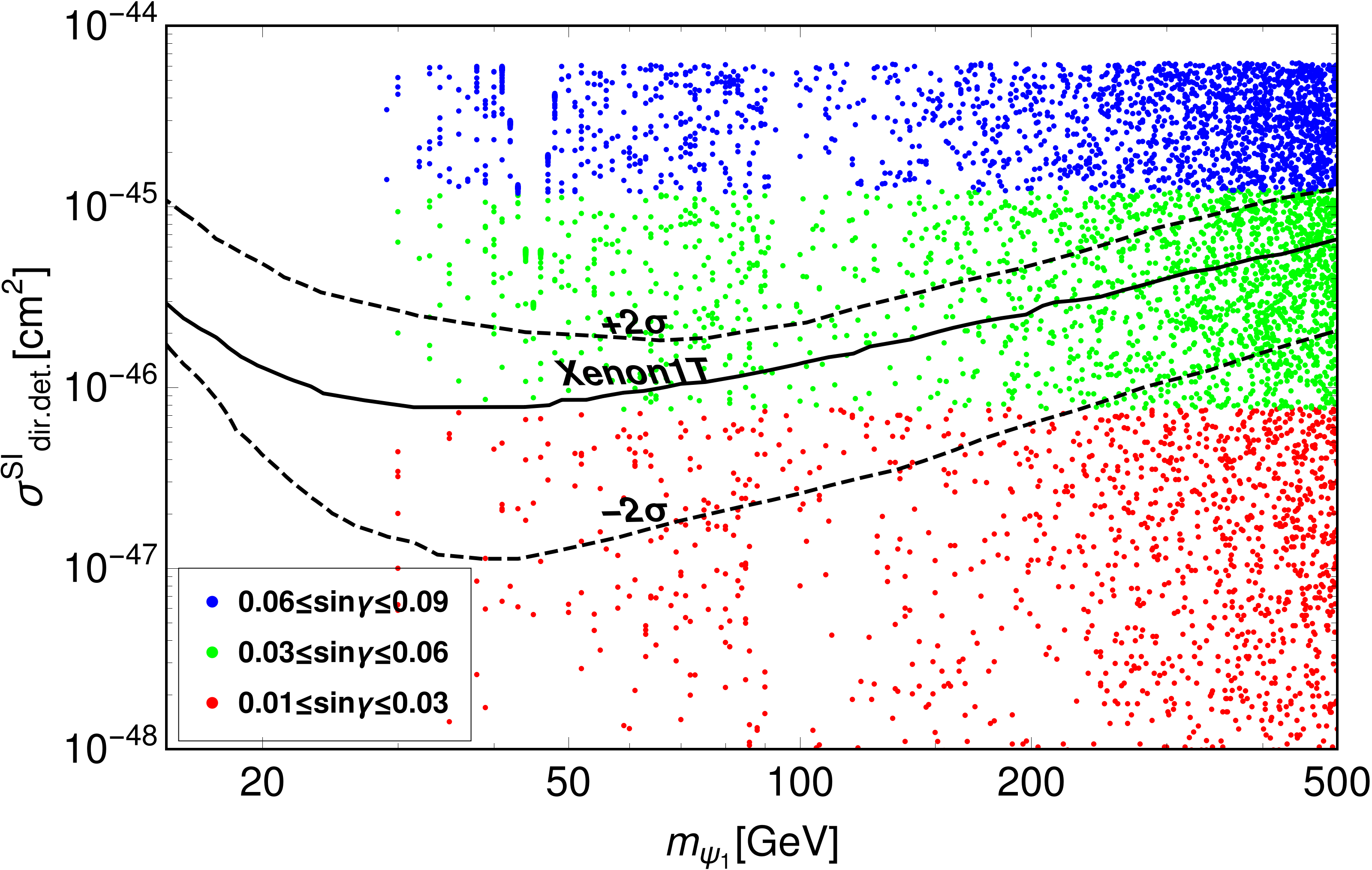
The strongest limits on the model parameters come from dark matter constraints. The interactions in Eq. (26) show that the DM relic density is determined by the $h$ and $Z$ -mediated annihilation and co-annihilation channels, while nuclear scattering, probed by direct-search experiments, is dominated by the $Z$ exchange process alone. The experimental constraint on the spin-independent cross section $\sigma^{\tt SI}_{\tt dir.\,det.}\lesssim 10^{-47}\rm{cm}^{2}$ (XENON1T collaboration, Aprile:2018dbl), and the fact that this cross section is $\propto\sin^{4}\gamma$ gives

\sin\gamma\lesssim 0.05~;

(27)

with a weak dependence on the DM mass. This limit on $\sin\gamma$ sharply reduces DM annihilation cross-section via $Z$ mediation, and also via Higgs portal interactions since $Y_{1}\propto\sin(\gamma)$ . Though the SM $\rightarrow$ DM annihilation channels are suppressed, the relic-abundance restriction ⁹⁹ 9 Here h denotes the Hubble parameter in units of $100\,$ km s^-1 Mpc^-1. $\Omega_{\tt DM}{\sf h}^{2}=0.11933\pm 0.00091$ (PLANCK collaboration Ade:2013zuv; Aghanim:2018eyx) can still be met through co-annihilation channels involving $\psi^{\pm}$ , provided $|\Delta m|\ll m_{\psi^{\pm}}$ Bhattacharya:2018cgx.

Fig. 9 displays various regions allowed by the direct-detection and relic-density constraints. The top panel displays the spin-independent direct-detection cross-section $\sigma^{\tt SI}_{\tt DD}$ a function of DM mass ( $m_{\psi_{1}}$ ) for various ranges of $\sin\gamma$ . The allowed region in the $m_{\psi_{1}}-\Delta m$ plane is displayed in the bottom left panel, while the allowed region in the $m_{\psi_{1}}-\sin\gamma$ plane for several ranges of $\Delta m$ is displayed on the right bottom panel of that figure. The parabola-like region in the bottom left panel is responsible for having two allowed values of $m_{\psi_{1}}$ for each choice of $\Delta m$ range on the right bottom panel; this paraboloid shape can be traced to the contribution from co-annihilation channels $\psi^{\pm}\psi_{1}\rightarrow$ SM to the DM annihilation cross section:

\left\langle\sigma v\right\rangle_{\tt tot}\simeq\left\langle\sigma v\right\rangle_{\psi_{1}\bar{\psi_{1}}\rightarrow\rm SM}+\left\langle\sigma v\right\rangle_{\psi_{1}\psi^{\pm}\rightarrow\rm SM}\left(1+\frac{\Delta m}{m_{\psi_{1}}}\right)^{3/2}e^{-\Delta m/T}+\cdots

(28)

where $T$ denotes the temperature of the bath, and the ellipses indicate other co-annihilation channels (e.g. $\psi^{+}\psi^{-}\rightarrow$ SM, $\psi_{1}\bar{\psi_{2}}\rightarrow$ SM) with a stronger exponential suppression; for details, see Bhattacharya:2018fus. The relic density is then

\Omega_{\tt DM}{\sf h}^{2}=\left.\frac{1.09\times 10^{9}~{\rm GeV}^{-1}(m_{\psi_{1}}/T)}{{g_{*}}^{1/2}M_{\tt Pl}}\frac{1}{\left\langle\sigma v\right\rangle_{\tt tot}}\right|_{T=T_{f}};

(29)

where $x=T/m_{\psi_{1}}$ , $g_{*}$ denotes the effective relativistic degrees of freedom, $M_{\tt Pl}$ the Planck mass, and $T_{f}$ the value of $T$ at freeze-out. From these expressions it follows that for small $\Delta m$ the allowed values increase with $m_{\psi_{1}}$ , but only up to a point beyond which $\Delta m$ must drop to balance the the exponential suppression in Eq. (28).

Collider data also impose constraints on this model, with the strongest limits from those on production of chargino pairs Aad:2019vnb, or chargino and second neutralino production Aad:2019qnd, in supersymmetric theories. Chargino pair production is the exact parallel of the one we study below (see Fig. 11 with $\psi^{\pm}$ replaced by charginos, and $\psi_{1}$ by neutralinos), in the limit where the chargino is wino-dominated and the sneutrinos are heavy ¹⁰¹⁰ 10 The sneutrinos generate a $t$ -channel graph not present in our model, and other contributions to the charginos generate chiral couplings to the $W$ ., and assuming the on-shell production of charginos dominates the cross section. These SUSY limits give

m_{\psi_{2}}+115\,\hbox{GeV}\gtrsim m_{\psi^{\pm}}\quad\text{for}~250\,\hbox{GeV}>m_{\psi^{\pm}}>150\,\hbox{GeV}

(30)

which, for $m_{\psi^{\pm}}=150\,\hbox{GeV}\,(245\,\hbox{GeV})$ , requires $m_{\psi_{1}}>35\,\hbox{GeV}\,(111\,\hbox{GeV})$ . The model is also consistent with electroweak precision observables, and with the invisible decay widths for the Higgs and $Z$ boson whenever $m_{\psi_{1}}>m_{h}/2$ , which we assume.

With these constraints in mind, we select several benchmark points, listed in Table 4, where all constraints are obeyed and which we will use in our study of the model at the ILC; for these we also assumed $\Delta m<m_{W}$ , so that the decay of heavy fermion occurs via an off-shell $W$ . We will show that for such relatively small mass splitting there is better segregation of the signal from the SM background at the ILC. The benchmark points are compared with limits from ATLAS Aad:2019vnb; Aad:2019qnd ¹¹¹¹ 11 The limits from CMS CMS:2020bfa agree well with Fig. 10 and also allow the chosen benchmark points. in Fig. 10.

Benchmark Points	$m_{\psi^{\pm}}$ (GeV)	$m_{\psi_{1}}$ (GeV)	$\Delta m$ (GeV)
BP1	$245$	215	30
BP2	$245$	207	38
BP3	$150$	117	33
BP4	$150$	110	40

Table 4: Benchmark points chosen for collider analysis for singlet-doublet fermion model; in all cases we took

\sin\gamma=0.05

4.1 Simulation of collider events

We now turn to the ILC collider signatures for this model for the chosen benchmark points (table 4) using the simplest signal: $\psi^{\pm}$ on-shell pair production with their subsequent decay into DM + opposite-sign leptons (OSL) via off-shell $W$ bosons (Fig. 11); we adopt the above mass hierarchy, $m_{\psi_{2}}>m_{\psi^{\pm}}>m_{\psi_{1}}$ . We note that $\psi_{1}\,\psi_{2}$ production, followed by $\psi_{2}\rightarrow Z\psi_{1}$ generates a similar final state (OSL plus missing energy), but the cross is $\propto\sin^{4}\gamma$ and significantly smaller. It is also possible to pair produce $\psi_{1},\,\psi_{2}$ but the final state signature is different.

We simulated OSL events at the ILC with $\sqrt{s}=500$ GeV as follows: the model was implemented in Feynrules Alloul:2013bka, and parton-level signal events were generated using CalcHEP Belyaev:2012qa, and then showered and analyzed using Pythia Sjostrand:2006za; SM background events were generated using MadGraph Alwall:2014hca and showered using Pythia. For event reconstruction, we use the following criteria:

•

Leptons are required to have at least transverse momentum $p_{T}>10$ GeV; we consider only electrons and muons with pseudorapidity $|\eta|<2.4$ – we do not consider $\tau$ signals. Two leptons are assumed isolated if $\Delta R_{\ell\ell}=\sqrt{(\Delta\eta)^{2}+(\Delta\phi)^{2}}\geq 0.2$ , while a lepton and a jet are assumed isolated if $\Delta R_{\ell j}\geq 0.4$ .
•

We impose a zero-jet requirement, where jets are reconstructed using the cone jet algorithm around initiating parton. We further require $p_{T}>20$ GeV and $|\eta|<3.0$ .
•

Background signal was minimized by imposing cuts at $20$ and $30$ GeV (see below) on the missing transverse energy, which is defined by

$E_{\tt T}^{\tt miss}=\left|{\bf p}^{\left(\tt vis\right)}_{\perp}\right|^{2}$ (31)

where ${\bf p}^{\left(\tt vis\right)}_{\perp}$ is the total visible momentum perpendicular to the beam direction.

Background	$\sigma^{\psi^{+}\psi^{-}}_{\tt SM}$ [pb]		$E_{\tt T}^{\tt miss}$ [GeV]	$\sigma^{\tt OSL}_{\tt SM}$ [fb]
	$P_{e^{\pm}}=0$	$P_{e^{\pm}}=^{+20\%}_{-80\%}$		$P_{e^{\pm}}=0$	$P_{e^{\pm}}=^{+20\%}_{-80\%}$
$WW$	$7.4$	$15.5$	$<20$	0.90	2.73
			$<30$	0.90	2.73
$WWZ$	$0.04$	$0.085$	$<20$	$5.3\times 10^{-4}$	$1.5\times 10^{-3}$
			$<$ 30	$1.6\times 10^{-3}$	$4.5\times 10^{-4}$
$ZZ$	$0.41$	$0.66$	$<20$	$3.1\times 10^{-3}$	$9.4\times 10^{-3}$
			$<30$	$4.7\times 10^{-3}$	$1.4\times 10^{-2}$

Table 5: SM background cross sections for the

\psi^{\pm}

and OSL final states at the ILC with

\sqrt{s}

=500 GeV with the selection cuts adopted (see text), and for unpolarized and polarized beams (

P_{e^{\pm}}=^{+20\%}_{-80\%}

$\sigma^{\psi^{+}\psi^{-}}$ [pb]		BPs	$E_{\tt T}^{\tt miss}$ [GeV]	$\sigma^{\tt OSL}$ [fb]		Efficiency ( $\epsilon$ )
$P_{e^{\pm}}=0$	$P_{e^{\pm}}=^{+20\%}_{-80\%}$	BPs	$E_{\tt T}^{\tt miss}$ [GeV]	$P_{e^{\pm}}=0$	$P_{e^{\pm}}=^{+20\%}_{-80\%}$	$P_{e^{\pm}}=0$	$P_{e^{\pm}}=^{+20\%}_{-80\%}$
$0.14$	$0.32$	BP1	$<20$	0.93	2.35	$6.43\times 10^{-3}$	$6.70\times 10^{-3}$
		BP1	$<30$	0.98	2.50	$6.98\times 10^{-3}$	$7.11\times 10^{-3}$
		BP2	$<20$	0.70	1.80	$5.00\times 10^{-3}$	$5.62\times 10^{-3}$
		BP2	$<30$	0.73	1.88	$5.21\times 10^{-3}$	$5.87\times 10^{-3}$
$0.45$	$1.13$	BP3	$<20$	2.97	7.92	$6.60\times 10^{-3}$	$7.00\times 10^{-3}$
		BP3	$<30$	3.32	8.45	$7.37\times 10^{-3}$	$7.47\times 10^{-3}$
		BP4	$<20$	2.30	6.05	$5.09\times 10^{-3}$	$5.36\times 10^{-3}$
		BP4	$<30$	2.40	6.32	$5.30\times 10^{-3}$	$5.60\times 10^{-3}$

Table 6: Signal (OSL) and

\psi^{\pm}

pair production cross sections and associated signal efficiency

\epsilon

Eq. (32) at the ILC for

\sqrt{s}=500

GeV with two missing-energy selection cuts and other selection cuts (see text) for unpolarized and polarized beams (

P_{e^{\pm}}=^{+20\%}_{-80\%}

Benchmark	$E_{\tt T}^{\tt miss}$	$\sigma^{\tt signal}$ [fb]
Points	[GeV]	OSL + 0 photon		OSL+ $\leq$ 1 photon		OSL+ $\leq$ 2 photon
		$P_{e^{\pm}}=0$	$P_{e^{\pm}}=^{+20\%}_{-80\%}$	$P_{e^{\pm}}=0$	$P_{e^{\pm}}=^{+20\%}_{-80\%}$	$P_{e^{\pm}}=0$	$P_{e^{\pm}}=^{+20\%}_{-80\%}$
BP1	$<20$	0.76	2.17	0.84	2.26	0.93	2.35
BP1	$<30$	0.80	2.31	0.87	2.39	0.98	2.50
BP2	$<20$	0.55	1.79	0.62	1.76	0.70	1.80
BP2	$<30$	0.60	1.71	0.67	1.79	0.73	1.88
BP3	$<20$	2.82	7.70	2.90	7.81	2.97	7.92
BP3	$<30$	2.15	8.21	2.24	8.33	3.32	8.45
BP4	$<20$	2.17	5.87	2.23	5.95	2.30	6.05
BP4	$<30$	2.26	6.16	2.34	6.23	2.40	6.32

Table 7: Signal cross-section including ISR and FSR photon count.

We present in Fig. 12 the missing transverse energy ( $E_{\tt T}^{\tt miss}$ ) distributions (normalized to one event) at the benchmark points for both the signal and the dominant SM background processes events ( $WW,\,WWZ,\,ZZ$ ); and for both polarized and unpolarized beams. Since the intermediate $W$ bosons are off shell, the peak of the missing energy distribution for the signal is at a much smaller value than those SM background, where $W$ production is on-shell. Based on these distributions we choose upper cuts $E_{\tt T}^{\tt miss}<20,\,30\,\hbox{GeV}$ ¹²¹² 12 ILC projections indicate this collider will be able to measure missing energy very accurately, so that the cut used in our analysis is viable Behnke:2013xla., which retain a significant part of the signal and eliminate most background events, as illustrated in Table 5.

The values of the $\psi^{\pm}$ pair production and signal event cross sections ( $\sigma^{\psi^{+}\psi^{-}}$ and $\sigma^{\tt OSL}$ , respectively) after imposing the above selection criteria and $E_{\tt T}^{\tt miss}$ cuts are given in Table 6 for both unpolarized and polarized ( $P_{e^{\pm}}=^{+20\%}_{-80\%}$ ) beams. Following the discussion in Sect. 2 we define

\displaystyle\epsilon=\frac{\sigma^{\tt OSL}}{\sigma^{\psi^{+}\psi^{-}}}~,

(32)

(see Eq. (6)) whose values are listed in Table 6. It is clear that $\epsilon\sim 0.001$ used throughout the previous OOT analysis is a conservative choice ( $\epsilon\sim 0.005$ more closely corresponds to the results derived in this section).

We also note that signal events are often accompanied with initial state radiation (ISR) and final state radiation (FSR) photons simulated with inbuilt functions in Pythia event generator. Using the photon selection criteria $p^{\tt photon}_{T}>5\,\hbox{GeV}$ and $|\eta_{\tt photon}|<0.24$ , the signal cross-section with zero photons, and the inclusive $\leq 1,\,2$ photon cross sections are listed in table 7. From this we can see that the inclusive diphoton cross sections match quite accurately the signal cross-section without photon tagging listed in Table 6¹³¹³ 13 With three photon and four photon events being very rare, inclusive di-photon event counts match quite accurately to signal cross-section without photon tagging as in Table 6..

We determine the discovery potential of the OSL signal at the ILC by plotting signal significance ( $S/\sqrt{S+B}$ , where $S$ and $B$ denote, respectively the number of signal and SM background events), as a function of luminosity ${\cal L}$ . The results are presented in Fig. 13; of particular interest is the advantage provided by using polarized beams, which require a lower luminosity for either the discovery or exclusion of the selected signal; in either case the design luminosity (cf. Eq. (3)) will be sufficient to exclude or detect the NP signal here investigated.

It is intriguing to investigate whether the optimal uncertainty of the NP parameters obtained in the preceding section can be realized in a collider environment given the SM background contribution as analyzed in model specific scenario here. The experimental determination of model parameters will depend on the choice of signatures, the selection criteria and the corresponding significance; the authors are unaware of such a study, but the required dedicated analysis lies beyond the scope of the present paper. We will return to this issue in a future publication.

5 Summary and Conclusions

In this paper, we have analyzed the optimal statistical determination of the parameters of physics beyond the Standard Model, using as a specific example the production of a new heavy charged fermion $\psi^{\pm}$ that can couple to the $Z$ boson and photon. We assumed for simplicity that the photon coupling is known, and allowing for both vector and axial coupling to the $Z$ with couplings $a$ and $b$ respectively. The optimal observable technique generates the minimal statistic uncertainty to which the couplings $a,\,b$ can be determined. We find that uncertainties for the case where $|a|\sim 1$ are roughly independent of the value of $b$ and smaller than those for the quasi-axial case $|a|\ll 1$ . Find find, in addition, that, as expected, beam polarization allows for a different distinction of these couplings.

We also studied a sample model where the vector-like case ( $b=0$ ) is realized; the model consists of an extension of the SM by a fermion isodoublet and a fermion singlet, both assumed odd under a ${\mathbbm{Z}}_{2}$ symmetry. In addition to providing a realization of the more general optimal observable analysis, this model contains a viable DM candidate. the presence of which can be probed at the ILC though $\psi^{\pm}$ pair production followed by their decays into DM and $W$ bosons. The analysis shows that given the expected ILC luminosity (Eq. (3)) this collider will provide early evidence (or provide an early exclusion) of the model here proposed, and that this collider will be able to measure the model parameters with an accuracy very close to the optimal one. It is worth noting that the analysis is applicable to supersymmetric chargino pair production in the limit of heavy sneutrino, including our results on the optimal statistical uncertainties for the charged-lepton couplings to the $Z$ in the $a\neq 0,b=0$ case.

Acknowledgements.

SB acknowledges grant CRG/2019/004078 from SERB, Govt. of India and Mr. Abdur Rouf with whom the project was initiated. SJ would like to acknowledge Dr. Basabendu Barman and Dr. Sunando Patra for technical help.

Appendix A Derivation of the optimal covariance matrix

Consider the observable as differential production cross section involving NP, which takes the form

\mathcal{O}=\frac{d\sigma_{\tt theo}}{d\phi}=\sum_{i}c_{i}f_{i}(\phi)\,,

(33)

where $c_{i}$ denote functions of NP parameters and $f_{i}$ a corresponding set of functions of the phase-space coordinates $\phi$ . The goal is to provide observables with which to measure the $c_{i}$ optimally.

The total cross section for the process is

\Sigma_{\tt theo}=\left\langle\frac{d\sigma_{\tt theo}}{d\phi}\right\rangle\,.

(34)

where, to simplify notation, we defined the bracket $\left\langle\cdots\right\rangle$ such that for any quantity $W$ depending on $\phi$ ,

\displaystyle\left\langle W\right\rangle=\int d\phi\,W(\phi)\,.

(35)

Next, if ${\mathfrak{L}}_{\tt int}$ is the integrated luminosity over prescribed period, the event rate ${\mathfrak{N}}_{\tt theo}$ is given by

{\mathfrak{N}}_{\tt theo}={\mathfrak{L}}_{\tt int}\Sigma_{\tt theo}\,.

(36)

With this definitions, the probability density function for observing $A$ events at phase-space points $\phi_{a}\,(a=1,\ldots,A)$ is given by

{\mathfrak{F}}_{\tt theo}(A;\Phi_{A})=\frac{e^{-{\mathfrak{N}}_{\tt theo}}}{A!}\prod_{a=1}^{A}{\mathfrak{f}}_{\tt theo}(\phi_{a})\,,\quad\text{where}~~{\mathfrak{f}}_{\tt theo}(\phi_{a})={\mathfrak{L}}_{\tt int}\frac{d\sigma_{\tt theo}}{d\phi}(\phi_{a})={\mathfrak{L}}_{\tt int}\mathcal{O}(\phi_{a})\,;

(37)

and $\Phi_{A}=(\phi_{1},\ldots,\phi_{A})$ . Choose now a set of observables $\mathpzc{o}_{i}(\phi)$ and let

\mathpzc{O}_{i}(A;\Phi_{A})=\sum_{a=1}^{A}\mathpzc{o}_{i}(\phi_{a})\,.

(38)

In the following we will need the expectation values of quantities using ${\mathfrak{F}}_{\tt theo}$ as the probability density function. These averages involve an integration over phase-space variables and a summation over the number of events. To simplify notation we also define $\left\lgroup\!\cdots\!\right\rgroup$ such that for any quantity $U$ that depends on $A$ and $\Phi_{A}$ ,

\left\lgroup\!U\!\right\rgroup=\sum_{A=0}^{\infty}\int d\Phi_{A}U(A;\Phi_{A})=\sum_{A=0}^{\infty}\int\prod_{c=1}^{A}d\phi_{c}U(A;\Phi_{A})\,.

(39)

Now, the normalization of the probability density function ( ${\mathfrak{F}}_{\tt theo}$ ) is given by,

$\displaystyle\left\lgroup\!{\mathfrak{F}}_{\tt theo}\!\right\rgroup=$	$\displaystyle\sum_{A=0}^{\infty}\int d\Phi_{A}\frac{e^{-{\mathfrak{N}}_{\tt theo}}}{A!}\prod_{a=1}^{A}{\mathfrak{f}}_{\tt theo}(\phi_{a})$
$\displaystyle=$	$\displaystyle\sum_{A=0}^{\infty}\int\frac{e^{-{\mathfrak{N}}_{\tt theo}}}{A!}\prod_{c=1}^{A}d\phi_{c}\prod_{a=1}^{A}{\mathfrak{f}}_{\tt theo}(\phi_{a})$
$\displaystyle=$	$\displaystyle\sum_{A=0}^{\infty}\int\frac{e^{-{\mathfrak{N}}_{\tt theo}}}{A!}d\phi_{1}d\phi_{2}...d\phi_{A}{\mathfrak{f}}_{\tt theo}(\phi_{1}){\mathfrak{f}}_{\tt theo}(\phi_{2})...{\mathfrak{f}}_{\tt theo}(\phi_{A})$
$\displaystyle=$	$\displaystyle\sum_{A=0}^{\infty}\frac{e^{-{\mathfrak{N}}_{\tt theo}}}{A!}\int{\mathfrak{f}}_{\tt theo}(\phi_{1})d\phi_{1}\int{\mathfrak{f}}_{\tt theo}(\phi_{2})d\phi_{2}...\int{\mathfrak{f}}_{\tt theo}(\phi_{A})d\phi_{A}$
$\displaystyle=$	$\displaystyle\sum_{A=0}^{\infty}\frac{e^{-{\mathfrak{N}}_{\tt theo}}}{A!}{\mathfrak{N}}_{\tt theo}^{A}\qquad$
$\displaystyle=$	$\displaystyle e^{-{\mathfrak{N}}_{\tt theo}}\underbrace{\sum_{A=0}^{\infty}\frac{{\mathfrak{N}}_{\tt theo}^{A}}{A!}}_{e^{{\mathfrak{N}}_{\tt theo}}}$
$\displaystyle=$	$\displaystyle 1.$	(40)

With these preliminaries the average of $\mathpzc{O}_{i}$ is

\left\lgroup\!{\mathfrak{F}}_{\tt theo}\mathpzc{O}_{i}\!\right\rgroup=\sum_{A=1}^{\infty}\frac{e^{-{\mathfrak{N}}_{\tt theo}}}{A!}{\mathfrak{N}}_{\tt theo}^{A-1}A\left\langle{\mathfrak{f}}_{\tt theo}\mathpzc{o}_{i}\right\rangle=\left\langle{\mathfrak{f}}_{\tt theo}\mathpzc{o}_{i}\right\rangle={\mathfrak{L}}_{\tt int}\left\langle\mathpzc{o}_{i}f_{j}\right\rangle c_{j}\,.

(41)

Let then

\Gamma_{i}=\left(M^{-1}\right)_{ij}\mathpzc{O}_{j}\,,\quad\text{where}\quad M_{ij}={\mathfrak{L}}_{\tt int}\left\langle\mathpzc{o}_{i}f_{j}\right\rangle\,,

(42)

in which case

c_{i}=\left\lgroup\!{\mathfrak{F}}_{\tt theo}\Gamma_{i}\!\right\rgroup\,.

(43)

Therefore, any $\Gamma_{i}$ that has the above form can be used to determine the $c_{i}$ . The idea now is to choose the $\Gamma_{i}$ that has the smallest covariance matrix.

The covariance matrix is given by

\displaystyle V_{ij}

\displaystyle=\left\lgroup\!{\mathfrak{F}}_{\tt theo}\Gamma_{i}^{\prime}\Gamma_{j}^{\prime}\!\right\rgroup=\left\lgroup\!{\mathfrak{F}}_{\tt theo}\Gamma_{i}\Gamma_{j}\!\right\rgroup-c_{i}c_{j}\,;\quad\text{where}~~\Gamma_{i}^{\prime}=\Gamma_{i}-c_{i};

(44)

which we extremize as a function of the $\mathpzc{o}_{i}$ . To this end we vary $a_{i}a_{j}V_{ij}$ (where the $a_{i}$ are for arbitrary constants) as a function of the $\mathpzc{o}_{i}$ :

\delta\left(\frac{1}{2}a_{i}a_{j}V_{ij}\right)=\left\lgroup\!{\mathfrak{F}}_{\tt theo}(b\mathpzc{O})\left(b_{i}\,\delta\!\mathpzc{O}_{i}-b_{i}\,\delta M_{ij}\,\Gamma_{j}\right)\!\right\rgroup=0\,,

(45)

where $b_{i}=a_{j}(M^{-1})_{ji}$ . Now one can show,

	$\displaystyle\left\lgroup\!{\mathfrak{F}}_{\tt theo}\mathpzc{O}_{k}\,\delta\mathpzc{O}_{i}\!\right\rgroup$	$\displaystyle=\int d\Phi\sum_{A=1}^{\infty}\frac{e^{-{\mathfrak{N}}_{\tt theo}}}{A!}\prod_{a=1}^{A}{\mathfrak{f}}_{\tt theo}(\phi_{a})\sum_{b=1}^{A}\mathpzc{o}_{k}(\phi_{b})\sum_{c=1}^{A}\delta\mathpzc{o}_{i}(\phi_{c})$
		$\displaystyle=\left\langle{\mathfrak{f}}_{\tt theo}\mathpzc{o}_{k}\delta\!\mathpzc{o}_{i}\right\rangle+\left\langle{\mathfrak{f}}_{\tt theo}\mathpzc{o}_{k}\right\rangle\left\langle{\mathfrak{f}}_{\tt theo}\delta\!\mathpzc{o}_{i}\right\rangle\,.$		(46)

Similarly,

\displaystyle\left\lgroup\!{\mathfrak{F}}_{\tt theo}\mathpzc{O}_{k}\Gamma_{j}\!\right\rgroup

\displaystyle=M^{-1}_{jl}\left\langle{\mathfrak{f}}_{\tt theo}\mathpzc{o}_{k}\mathpzc{o}_{l}\right\rangle+\left\langle{\mathfrak{f}}_{\tt theo}\mathpzc{o}_{k}\right\rangle c_{j}.

(47)

where we used $M^{-1}_{jl}\left\langle{\mathfrak{f}}_{\tt theo}\mathpzc{o}_{l}\right\rangle=c_{j}$ . The extremum condition then reads

\displaystyle b_{i}b_{k}\bigg\{{\mathfrak{f}}_{\tt theo}\mathpzc{o}_{k}+\left\langle{\mathfrak{f}}_{\tt theo}\mathpzc{o}_{k}\right\rangle{\mathfrak{f}}_{\tt theo}-{\mathfrak{L}}_{\tt int}f_{j}\left[M^{-1}_{jl}\left\langle{\mathfrak{f}}_{\tt theo}\mathpzc{o}_{k}\mathpzc{o}_{l}\right\rangle+\left\langle{\mathfrak{f}}_{\tt theo}\mathpzc{o}_{k}\right\rangle c_{j}\right]\bigg\}=0.

(48)

Then, since $b_{i}b_{k}\neq 0$ as $a$ is arbitrary and ${\mathfrak{L}}_{\tt int}\sum_{j}f_{j}c_{j}={\mathfrak{f}}_{\tt theo}$ , the solution is

{\mathfrak{f}}_{\tt theo}\mathpzc{o}_{k}={\mathfrak{L}}_{\tt int}f_{j}M^{-1}_{jl}\left\langle{\mathfrak{f}}_{\tt theo}\mathpzc{o}_{k}\mathpzc{o}_{l}\right\rangle{\quad\Rightarrow\quad}\mathpzc{o}_{k}=\frac{f_{k}}{{\mathfrak{f}}_{\tt theo}}\,,

(49)

for which the condition $\left\langle f_{k}\right\rangle=M_{kl}c_{l}$ is satisfied and the optimal covariance matrix is then

V=\frac{1}{{\mathfrak{L}}_{\tt int}}M^{-1}\,;\qquad M_{ij}={\mathfrak{L}}_{\tt int}\left\langle\frac{f_{i}f_{j}}{{\mathfrak{f}}_{\tt theo}}\right\rangle=\left\langle\frac{f_{i}f_{j}}{\mathcal{O}}\right\rangle\,.

(50)

Appendix B Optimal Analysis with other CM energies (unpolarized beams)

In this appendix we repeat the analysis of Sect. 3.2 for both lower and higher CM energies and different charged-fermion masses. The results are presented in Fig. 14: OOT $1$ - $\sigma$ regions for $\sqrt{s}=250\,\hbox{GeV},~m_{\psi^{\pm}}=110$ GeV (left column), and $\sqrt{s}=2\,\hbox{TeV},~m_{\psi^{\pm}}=900$ GeV (right column). Note that as $m_{\psi^{\pm}}$ and $s$ increase the cross-section drops (Drell-Yann process falls like $\sim 1/\sqrt{s}$ , see Eq. (12)) and the eigenvalues of the covariance matrix increase (since $V^{-1}\sim M\sim 1/\sigma$ , cf. Eqs. (2), (3), and (5)); the $1$ - $\sigma$ regions are corresponding larger. The two cases where $a,b\neq 0$ , the 1 $\sigma$ regions are very asymmetric because the probability distribution of NP couplings are heavily distorted from the normal distribution.

Appendix C $\chi^{2}$ ellipsoids in $c_{i}$ plane

If the $c_{i}$ are taken as the NP parameters, then the $\chi^{2}=1$ regions become ellipsoids in this space, as illustrated in Fig. 15 for two examples. In general $V_{0}$ in Eq. (5) is not diagonal, so that the $c_{i}$ ’s are correlated, however, one can always choose alternative coefficients, linear combinations of the $c_{i}$ , which are uncorrelated and whose ( $1\sigma$ ) statistical uncertainties equal the square-root of the eigenvalues of $V_{0}$ . That is, if $c_{i}=R_{ij}\tilde{c}_{i}$ , one can always find $R$ orthogonal which diagonalizes $V_{0}$ , whence Eq. (5) becomes $\chi^{2}=\epsilon\sum(\delta\tilde{c}_{i})^{2}/\bar{V}^{i}_{0}$ , where the eigenvalues of $V_{0}$ are denoted by $\bar{V}_{0}^{i}$ and $\delta\tilde{c}_{i}$ is the statistical uncertainty of the $\bar{c}_{i}$ . An example is given in Table 8 and corresponding 1 $\sigma$ ellipsoids are shown in Fig. 15.

	Uncertainties $\times 10^{-6}$ ( $\epsilon=0.001$ )			Uncertainties $\times 10^{-6}$ ( $\epsilon=0.005$ )
Seed parameters $\times 10^{-5}$	$\quad\|\delta\tilde{c}_{1}\|\quad$	$\quad\|\delta\tilde{c}_{2}\|\quad$	$\quad\|\delta\tilde{c}_{3}\|\quad$	$\quad\|\delta\tilde{c}_{1}\|\quad$	$\quad\|\delta\tilde{c}_{2}\|\quad$	$\quad\|\delta\tilde{c}_{3}\|\quad$
$c^{0}_{1}=c^{0}_{2}=1;\,c_{3}^{0}=1$	$1.07$	$18.40$	$179.06$	$0.48$	$8.23$	$80.07$
$c^{0}_{1}=c_{2}^{0}=1;\,c_{3}^{0}=-1$	$1.06$	$18.18$	$177.16$	$0.47$	$8.13$	$79.23$

Table 8:

1\sigma

statistical uncertainties for the uncorrelated parameters

\tilde{c}_{i}

(see text) for the indicated seed parameters and efficiencies; we assume unpolarized beams.

Appendix D 68% C.L. in two-parameter and three-parameter distributions

As noted below Eq. (5) in Sect. 2, when the model has $n$ normally-distributed parameters, the C.L. for $\chi^{2}\leq\ell$ equals $\left(1-\Gamma(n/2,\ell/2)/\Gamma(n/2)\right)$ . For example, if $n=2\,(3)$ , a 68% C.L. corresponds to $\ell=2.3\,(3.5)$ . The 68% C.L. contours are plotted in Fig. 16 when $a_{0}=b_{0}=1$ (left panel) and for $c_{i}^{0}=10^{-5}$ (right panel); a comparison with the $\chi^{2}\leq 1$ region is also provided. It is quite evident that 68% C.L. regions are larger than 1 $\sigma$ surfaces.

References

(1) ATLAS collaboration, Observation of a new particle in the search for the Standard Model Higgs boson with the ATLAS detector at the LHC, Phys. Lett. B 716 (2012) 1 [1207.7214].
(2) CMS collaboration, Observation of a New Boson at a Mass of 125 GeV with the CMS Experiment at the LHC, Phys. Lett. B 716 (2012) 30 [1207.7235].
(3) BaBar collaboration, Evidence for an excess of $\bar{B}\rightarrow D^{(*)}\tau^{-}\bar{\nu}_{\tau}$ decays, Phys. Rev. Lett. 109 (2012) 101802 [1205.5442].
(4) LHCb collaboration, Measurement of the ratio of branching fractions $\mathcal{B}(B_{c}^{+}\,\rightarrow\,J/\psi\tau^{+}\nu_{\tau})$ / $\mathcal{B}(B_{c}^{+}\,\rightarrow\,J/\psi\mu^{+}\nu_{\mu})$ , Phys. Rev. Lett. 120 (2018) 121801 [1711.05623].
(5) BaBar collaboration, Measurement of an Excess of $\bar{B}\rightarrow D^{(*)}\tau^{-}\bar{\nu}_{\tau}$ Decays and Implications for Charged Higgs Bosons, Phys. Rev. D 88 (2013) 072012 [1303.0571].
(6) LHCb collaboration, Test of Lepton Flavor Universality by the measurement of the $B^{0}\rightarrow D^{*-}\tau^{+}\nu_{\tau}$ branching fraction using three-prong $\tau$ decays, Phys. Rev. D 97 (2018) 072013 [1711.02505].
(7) LHCb collaboration, Test of lepton universality in beauty-quark decays, 2103.11769.
(8) Muon g-2 collaboration, Measurement of the positive muon anomalous magnetic moment to 0.7 ppm, Phys. Rev. Lett. 89 (2002) 101804 [hep-ex/0208001].
(9) Muon g-2 collaboration, Final Report of the Muon E821 Anomalous Magnetic Moment Measurement at BNL, Phys. Rev. D 73 (2006) 072003 [hep-ex/0602035].
(10) T. Aoyama, M. Hayakawa, T. Kinoshita and M. Nio, Complete Tenth-Order QED Contribution to the Muon g-2, Phys. Rev. Lett. 109 (2012) 111808 [1205.5370].
(11) T. Aoyama et al., The anomalous magnetic moment of the muon in the Standard Model, Phys. Rept. 887 (2020) 1 [2006.04822].
(12) Muon g-2 collaboration, Measurement of the Positive Muon Anomalous Magnetic Moment to 0.46 ppm, Phys. Rev. Lett. 126 (2021) 141801 [2104.03281].
(13) T. Behnke, J. E. Brau, B. Foster, J. Fuster, M. Harrison, J. M. Paterson et al., The International Linear Collider Technical Design Report - Volume 1: Executive Summary, 1306.6327.
(14) L3 collaboration, Search for heavy neutral and charged leptons in $e^{+}e^{-}$ annihilation at LEP, Phys. Lett. B 517 (2001) 75 [hep-ex/0107015].
(15) Particle Data Group collaboration, Review of Particle Physics, Phys. Rev. D 98 (2018) 030001.
(16) CMS collaboration, Search for Evidence of the Type-III Seesaw Mechanism in Multilepton Final States in Proton-Proton Collisions at $\sqrt{s}=13\text{ }\text{ }\mathrm{TeV}$ , Phys. Rev. Lett. 119 (2017) 221802 [1708.07962].
(17) CMS collaboration, Searches for Long-Lived Charged Particles in $pp$ Collisions at $\sqrt{s}$ =7 and 8 TeV, JHEP 07 (2013) 122 [1305.0491].
(18) ATLAS collaboration, Search for electroweak production of charginos and sleptons decaying into final states with two leptons and missing transverse momentum in $\sqrt{s}=13$ TeV $pp$ collisions using the ATLAS detector, Eur. Phys. J. C 80 (2020) 123 [1908.08215].
(19) ATLAS collaboration, Searches for electroweak production of supersymmetric particles with compressed mass spectra in $\sqrt{s}=$ 13 TeV $pp$ collisions with the ATLAS detector, Phys. Rev. D 101 (2020) 052005 [1911.12606].
(20) D. Atwood and A. Soni, Analysis for magnetic moment and electric dipole moment form-factors of the top quark via $e^{+}e^{-}$ — $>$ $t\bar{t}$ , Phys. Rev. D 45 (1992) 2405.
(21) M. Davier, L. Duflot, F. Le Diberder and A. Rouge, The Optimal method for the measurement of tau polarization, Phys. Lett. B 306 (1993) 411.
(22) M. Diehl and O. Nachtmann, Optimal observables for the measurement of three gauge boson couplings in $e^{+}e^{-}$ — $>$ $W^{+}W^{-}$ , Z. Phys. C 62 (1994) 397.
(23) J. F. Gunion, B. Grzadkowski and X.-G. He, Determining the $t\bar{t}$ and $ZZ$ couplings of a neutral Higgs boson of arbitrary CP nature at the NLC, Phys. Rev. Lett. 77 (1996) 5172 [hep-ph/9605326].
(24) A. Das, S. Mandal and T. Modak, Testing triplet fermions at the electron-positron and electron-proton colliders using fat jet signatures, Phys. Rev. D 102 (2020) 033001 [2005.02267].
(25) A. Das and S. Mandal, Bounds on the triplet fermions in type-III seesaw and implications for collider searches, Nucl. Phys. B 966 (2021) 115374 [2006.04123].
(26) K. Hagiwara, S. Ishihara, J. Kamoshita and B. A. Kniehl, Prospects of measuring general Higgs couplings at $e^{+}e^{-}$ linear colliders, Eur. Phys. J. C 14 (2000) 457 [hep-ph/0002043].
(27) S. Dutta, K. Hagiwara and Y. Matsumoto, Measuring the Higgs-Vector boson Couplings at Linear $e^{+}e^{-}$ Collider, Phys. Rev. D 78 (2008) 115016 [0808.0477].
(28) B. Grzadkowski and Z. Hioki, CP violating lepton energy correlation in $e^{-}e^{+}$ — $>$ $t\bar{t}$ , Phys. Lett. B 391 (1997) 172 [hep-ph/9608306].
(29) B. Grzadkowski, Z. Hioki and M. Szafranski, Four Fermi effective operators in top quark production and decay, Phys. Rev. D 58 (1998) 035002 [hep-ph/9712357].
(30) B. Grzadkowski and Z. Hioki, Probing top quark couplings at polarized NLC, Phys. Rev. D 61 (2000) 014013 [hep-ph/9805318].
(31) B. Grzadkowski and J. Pliszka, Testing top quark Yukawa interactions in $e^{+}e^{-}$ — $>$ $t\bar{t}Z$ , Phys. Rev. D 60 (1999) 115018 [hep-ph/9907206].
(32) B. Grzadkowski and Z. Hioki, Optimal observable analysis of the angular and energy distributions for top quark decay products at polarized linear colliders, Nucl. Phys. B 585 (2000) 3 [hep-ph/0004223].
(33) B. Grzadkowski, Z. Hioki, K. Ohkuma and J. Wudka, Probing anomalous top quark couplings induced by dimension-six operators at photon colliders, Nucl. Phys. B 689 (2004) 108 [hep-ph/0310159].
(34) B. Grzadkowski, Z. Hioki, K. Ohkuma and J. Wudka, Optimal-observable analysis of possible new physics using the b quark in $\gamma\gamma$ — $>$ $t\bar{t}$ — $>$ $bX$ , Phys. Lett. B 593 (2004) 189 [hep-ph/0403174].
(35) B. Grzadkowski, Z. Hioki, K. Ohkuma and J. Wudka, Optimal beam polarizations for new-physics search through $\gamma\gamma$ — $>$ $t\bar{t}$ — $>$ $lX/bX$ , JHEP 11 (2005) 029 [hep-ph/0508183].
(36) Z. Hioki, T. Konishi and K. Ohkuma, Studying possible CP-violating Higgs couplings through top-quark pair productions at muon colliders, JHEP 07 (2007) 082 [0706.4346].
(37) J. F. Gunion and J. Pliszka, Determining the relative size of the CP even and CP odd Higgs boson couplings to a fermion at the LHC, Phys. Lett. B 444 (1998) 136 [hep-ph/9809306].
(38) Z. Hioki and K. Ohkuma, Optimal-observable Analysis of Possible Non-standard Top-quark Couplings in $pp->t\bar{t}X->l^{+}X^{\prime}$ , Phys. Lett. B 716 (2012) 310 [1206.2413].
(39) Z. Hioki and K. Ohkuma, Final charged-lepton angular distribution and possible anomalous top-quark couplings in $pp\rightarrow t\bar{t}X\rightarrow\ell^{+}X^{\prime}$ , Phys. Lett. B 736 (2014) 1 [1406.2475].
(40) S. Bhattacharya, S. Nandi and S. K. Patra, Optimal-observable analysis of possible new physics in $B\rightarrow D^{(\ast)}\tau\nu_{\tau}$ , Phys. Rev. D 93 (2016) 034011 [1509.07259].
(41) Z. Calcuttawala, A. Kundu, S. Nandi and S. K. Patra, Optimal observable analysis for the decay $b\rightarrow s$ plus missing energy, Eur. Phys. J. C 77 (2017) 650 [1702.06679].
(42) Z. Calcuttawala, A. Kundu, S. Nandi and S. Kumar Patra, New physics with the lepton flavor violating decay $\tau\rightarrow 3\mu$ , Phys. Rev. D 97 (2018) 095009 [1802.09218].
(43) Q.-H. Cao and J. Wudka, Search for new physics via single top production at TeV energy e gamma colliders, Phys. Rev. D 74 (2006) 094015 [hep-ph/0608331].
(44) R. Vega and J. Wudka, A Covariant method for calculating helicity amplitudes, Phys. Rev. D 53 (1996) 5286 [hep-ph/9511318].
(45) S. Bhattacharya, N. Sahoo and N. Sahu, Minimal vectorlike leptonic dark matter and signatures at the LHC, Phys. Rev. D 93 (2016) 115040 [1510.02760].
(46) S. Bhattacharya, P. Ghosh, N. Sahoo and N. Sahu, Mini Review on Vector-Like Leptonic Dark Matter, Neutrino Mass, and Collider Signatures, Front. in Phys. 7 (2019) 80 [1812.06505].
(47) XENON collaboration, Dark Matter Search Results from a One Ton-Year Exposure of XENON1T, Phys. Rev. Lett. 121 (2018) 111302 [1805.12562].
(48) Planck collaboration, Planck 2013 results. XVI. Cosmological parameters, Astron. Astrophys. 571 (2014) A16 [1303.5076].
(49) Planck collaboration, Planck 2018 results. VI. Cosmological parameters, Astron. Astrophys. 641 (2020) A6 [1807.06209].
(50) S. Bhattacharya, P. Ghosh and N. Sahu, Multipartite Dark Matter with Scalars, Fermions and signatures at LHC, JHEP 02 (2019) 059 [1809.07474].
(51) CMS collaboration, Search for supersymmetry in final states with two oppositely charged same-flavor leptons and missing transverse momentum in proton-proton collisions at $\sqrt{s}=$ 13 TeV, JHEP 04 (2021) 123 [2012.08600].
(52) A. Alloul, N. D. Christensen, C. Degrande, C. Duhr and B. Fuks, FeynRules 2.0 - A complete toolbox for tree-level phenomenology, Comput. Phys. Commun. 185 (2014) 2250 [1310.1921].
(53) A. Belyaev, N. D. Christensen and A. Pukhov, CalcHEP 3.4 for collider physics within and beyond the Standard Model, Comput. Phys. Commun. 184 (2013) 1729 [1207.6082].
(54) T. Sjostrand, S. Mrenna and P. Z. Skands, PYTHIA 6.4 Physics and Manual, JHEP 05 (2006) 026 [hep-ph/0603175].
(55) J. Alwall, R. Frederix, S. Frixione, V. Hirschi, F. Maltoni, O. Mattelaer et al., The automated computation of tree-level and next-to-leading order differential cross sections, and their matching to parton shower simulations, JHEP 07 (2014) 079 [1405.0301].

Probing heavy charged fermions at 𝒆+​𝒆−e^{+}e^{-} collider using the Optimal Observable Technique