∎
VEER: Enhancing the Interpretability of Model-based Optimizations
Abstract
Background: Many software systems can be tuned for multiple objectives (e.g., faster runtime, less required memory, less network traffic or energy consumption, etc.). Such systems can suffer from “disagreement” where different models have different (or even opposite) insights and tactics on how to optimize a system. For configuration problems, we show that (a) model disagreement is rampant; yet (b) prior to this paper, it has barely been explored.
Goal: We aim at helping practitioners and researchers better solve multi-objective configuration optimization problems, by resolving model disagreement.
Method: We propose a dimension reduction method called VEER that builds a useful one-dimensional approximation to the original N-objective space. Traditional model-based optimizers use Pareto search to locate Pareto-optimal solutions to a multi-objective problem, which is computationally heavy on large-scale systems. VEER builds a surrogate that can replace the Pareto sorting step after deployment.
Results: Compared to the prior state-of-the-art, for 11 configurable systems, VEER significantly reduces disagreement and execution time, without compromising the optimization performance in most cases. For our largest problem (with tens of thousands of possible configurations), optimizing with VEER finds as good or better optimizations with zero model disagreements, three orders of magnitude faster.
Conclusion: When employing model-based optimizers for multi-objective optimization, we recommend to apply VEER, which not only improves the execution time, but also resolves the potential model disagreement problem.
Conflict of interest
We assert that the authors have no conflict of interest.
Keywords:
Software analytics Multi-objective optimization Disagreement Interpretable AI1 Introduction
One of the recent successes of AI for software engineering (SE) is automated configuration Kaltenecker et al. 2020. Software comes with many options as well as various objectives, and exploring all these configuration options for multiple objectives can be tedious, time consuming, and even error-prone (when done manually). Much recent work shows that AI tools can dramatically improve this procedure; for instance, regression tree learners can report what subset of the configuration options are most influential to achieving better performance Golovin et al. 2017; Chen et al. 2018b. Further, while it takes a long time to run the system with all possible (feasible) configuration settings, an incremental AI tool can reflect on the model learned so far to recommend what is the next most informative configuration to try Nair et al. 2018. This way, the time required to run enough configurations to effectively optimize software can be substantially reduced (e.g., as shown by the experiments of this paper, after running less than 100 configurations, we can optimize systems with nearly 90,000 configurations).
When business users ask “what has been learned from these models?”, we need interpretable models to offer comprehensible advice on how to best configure a system Sawyer 2011; Tan and Chan 2016; Chen et al. 2018a. But when software systems have multiple objectives (e.g., faster transaction response time, fewer memory requirements, decreased network traffic, decreased energy consumption, etc), such advice could clash. We call this the model disagreement problem: while one model shows some configuration options to be useful to achieve one objective, another model might argue that such options are actually detrimental to another objective. Table 1 shows examples of model disagreement. Later in this paper, we show that model disagreement is rampant in all our test cases (see our experimental results in §7).
| Project | Model 1 | Model 2 |
|---|---|---|
| SS-E | How to minimize runtime | How to minmize CPU load |
| columnTiling | columnTiling | |
| goodQuality | goodQuality | |
| AutoAltRef | AutoAltRef | |
| SS-F | How to minimize latency | How to maximize throughput |
| max_spout 0.55 | max_spout 0.05 | |
| chunk 0.14 | chunk 0.05 | |
| SS-G | How to minimize runtime | How to minimize CPU load |
| compressionZqap | compressionZqap | |
| compressionLzma | compressionLzma False | |
| processorCount 0.17 | processorCount 0.17 |
Looking at the literature, we find very little discussion on model disagreement. That is, model disagreement may be a long-standing, but previously under-explored, problem. This begs the questions “why has this problem not been reported before?” Perhaps other researchers were content to stop after generating multiple solutions (e.g., 10,000 solutions across the frontier of best solutions). In our work, however, we have been studying interpretation tools that offer clear advice on how to best configure a system. Hence, we prefer not to confuse users with a long list of candidate solutions. Instead, we prefer rule-based summaries (such as those seen in Table 1).
This paper tests the following conjecture. If multiple objectives complicate interpretations, then one possible solution is to:
(1) Reduce multi-dimensional objective space to a lower-dimensional space. (2) Reason in that reduced space.
We propose a tactic called VEER, which is applied as follows: (a) lay out all the configuration options as points in an N-dimensional objective space, then (b) rank the best point as “1”. After that, we “VEER” to the nearest best point P to rank it as “2”; and so on. The ranks found by VEERing across all the objectives are then used as a single-dimensional objective space. Configuration recommendations are then found by reasoning over this simpler space.
Overall, the contributions of this paper are:
- •
We verify the existence of the model disagreement problem in multi-objective software configuration.
- •
We show that model disagreement is not a simple problem that can be easily solved via some simplistic weighting mechanisms (e.g., a naive multi-regression approach).
- •
We propose a novel tactic to resolve the model disagreement problem and generate confusion-free model interpretations.
- •
We show that, since VEER is exploring a simpler goal space, it runs very fast (up to 1,000 times faster while at the same time recommending configuration solutions that are as good as or better than the prior state-of-the-art).
2 Background and Related Work
2.1 Why do configuration optimizations need “interpretation?”
This section argues the necessity of interpretability and transparency for configuration models, which motivates this paper.
Configurable software systems come with numerous options such that users can customize the system for their varying requirements. However, once a configuration space becomes large, users can easily get confused by possible interactions among configuration options with distinct impacts on diverse objectives. For example, many software systems have poorly chosen defaults Van Aken et al. 2017; Herodotou et al. 2011. Hence, it is useful to seek better configurations. Unfortunately, understanding the configuration space of software systems with large configuration spaces can be challenging Xu et al. 2015; Kolesnikov et al. 2019, and exploring more than just a handful of configurations is usually infeasible due to long benchmarking time Zhu et al. 2017.
When manual methods fail, automatic tools can be of assistance. In the case of configuration, those automatic tools are usually assessed with respect to the objectives of the system. Many prior works have demonstrated effectiveness in optimizing configurations for single-objective and multi-objective systems Siegmund et al. 2015; Guo et al. 2018; Song and Chan 2015. In this paper, while we focus on systems with more than one objectives, we add one more assessment criteria: transparency. A recent 2021 report by the Gartners group11 1 http://tiny.cc/gartners21 states
Responsible AI governance (and) transparency (our emphasis) … is the most valuable differentiator in this market, and every listed vendor is making progress in these areas.
A model with conflicting interpretations on different objectives is considered more of opaque than transparent. That is, model disagreement complicates transparency since users cannot directly and immediately understand the implications of multiple models, if those models disagree with each other. Hence, we seek for means to resolve such conflicting interpretations when it comes to optimizing a software system for multiple objectives.
We are concerned with transparency since, as shown in Figure 1, ML models that chase different goals might make different recommendations. Therefore, even if each of the machine learners is interpretable, it remains possible that the internals of different machine learners are disagreeing or conflicting with each other: For example, one model might offer an insight that increasing certain option can optimize an objective , while another model believes increasing such option will harm another objective . In Table 1, we present some examples of such disagreement observed from dataset explored in this paper.

2.2 What is a good interpretation?
Looking through the literature, we can find very little on how to handle model disagreement in multi-objective optimization tasks. The closest thing we have found to our work is the Clafer visualizer Antkiewicz et al. 2013 environment. In Clafer, when there is a trade-off among multiple objectives in an optimization problem, the users are asked to make the decision on the trade-off.
While Clafer improves practitioners’ understanding by visualizing the performance of different configuration candidates, such form of interpretations still has its limitations. Firstly, Clafer’s interpretations on how to optimize a configuration task is instance-based: While candidate configurations with various trade-off among multiple objectives are shown to users, no further insights are generalized by Clafer. In other words, users may be able to obtain a vague picture of what configuration options have positive influence on certain objective (in terms of performance measured), yet those options can usually be conflicting due to competing objectives (see examples in Table 1). In the end, there still lacks of conclusive agreement on which options should be preferred.
Secondly, the problem with human-centered approaches such as the Clafer visualizer is that a repeated empirical result illustrates that humans are very poor oracles for what best improves a project (e.g., in Devanbu’s ICSE’16 study Devanbu et al. 2016 on 500+ developers at Microsoft, even when developers work on the same project, they mostly make conflicting and/or incorrect conclusions about what factors most affect software quality; similar patterns were observe in Shrikanth’s ICSE-SEIP’20 study Shrikanth and Menzies 2020). Hence we seek methods that remove as much as possible those competing recommendations.
Regarding as much as possible, sometimes objectives are inherently opposed in their recommendation direction, due to the semantics of the domain. If this effect has the majority case, then the method of this paper would be doomed to fail. That said, the novel result of this paper is that at least for the data sets studied here, the objectives are not inherently apposed. Since we can generate a disagreement-free model to provide solutions that perform as well or better as those seen produced by other methods, this result should prompt much future work exploring emergent simplicity in multi-objective reasoning in SE.
| Name | Abbr. | Domain | #Options (B/N) | Performance Measures | ||
|---|---|---|---|---|---|---|
| HSQLDB | SS-A | SQL database | 15/0 | 864 | run time, energy, cpu load | 3 |
| MariaDB | SS-B | SQL database | 7/3 | 972 | run time, cpu load | 2 |
| wc-5d-c5 | SS-C | streaming process system | 0/5 | 1 080 | throughput, latency | 2 |
| VP8 | SS-D | video encoder | 7/4 | 2 736 | run time, energy, cpu load | 3 |
| VP9 | SS-E | video encoder | 9/3 | 3 008 | run time, cpu load | 2 |
| rs-6d-c3 | SS-F | streaming process system | 0/6 | 3 839 | throughput, latency | 2 |
| lrzip | SS-G | compression tool | 9/3 | 5 184 | run time, cpu load | 2 |
| x264 | SS-H | video encoder | 17/0 | 4 608 | run time, cpu load | 2 |
| MongoDB | SS-I | No-SQL database | 13/2 | 6 840 | run time, cpu load | 2 |
| LLVM | SS-J | compiler | 16/0 | 65 536 | run time, cpu load | 2 |
| ExaStencils | SS-K | Stencil code generator | 4/6 | 86 058 | run time, cpu load | 2 |
3 Details, Definitions and Algorithms
This section refines the motivation of this paper by defining the configuration optimization problem and reviewing prior works associated with the problem. Table 2 shows the datasets used in our experiments.
3.1 Configurable Software System (CSS)
In general, a configurable software system (CSS) contains a set of valid configurations . Let represent the th valid configuration and represent the th option in that configuration. In our case studies, the option is either a numerical parameter or a Boolean value. A numerical parameter (i.e., page size) has multiple different numerical values and Boolean values are indicating a certain option as enabled or disabled. A configurable software system also contains a set of performance measures (i.e., response time, energy consumption, etc.), where represents the th performance value of the th configuration in . Since we consider configurable systems with more than one performance measure, is always greater than 1. The configuration space is referred to as an independent variable while the performance measure space is referred to as a dependent variable (i.e., depends on ). Theoretically, to find an optimal configuration for a software system, we learn the relationship between and by approximating the function that maps configurations onto the performance (objective) space by . In real-world practice, the evaluations required to approximate the function , also referred to as measurements, are usually expensive and time-consuming. Therefore, in this paper, the cost of a configuration optimizer is referred to as the total amount of measurements taken to generate the optimal solutions (may not be actually “optima”, but one that an optimizer determines to be optimal).
While there always exists an optimal solution in a single-objective optimization task (where a better solution can be determined by a single criterion), there might not be any optimal solution in a multi-objective optimization task. This might be the situation where no configuration is best in all objectives. Therefore, we need to quantify and evaluate the overall quality of a configuration in a different manner, called the domination relationship. There are two major types of domination relationship: binary domination Holland 1992, and continuous domination Laumanns et al. 2002. According to the definition of binary domination, a configuration is binary dominant over iff:
| (1) |
In contrast, continuous domination defines that a configuration is dominant over iff:
| (2) |
where the loss function is defined as:
| (3) |
Note that in both equations above, the default setting is that the lower performance measure is preferred. By definitions, a best (optimal) configuration is one that is not dominated by any other configuration, denoted as a non-dominated solution. And the set containing all non-dominated solutions is called Pareto frontier set. In short, the goal in a multi-objective optimization problem is to find as many optimal (non-dominated) solutions as possible while minimizing the evaluation cost (using fewer measurements).
while do
while do
if dominates then
return
To compute the non-dominated solution set, the non-dominated sorting process is required, which has a runtime complexity of where is the number of objectives and is the population size. It is also noteworthy that NSGA-II Deb et al. 2002 proposed a fast and elitism sorting approach that reduced this complexity to . As described in Algorithm 1, this paper follow the same sorting process used in NSGA-II. This is important since our approach provides a faster workaround that only uses non-dominating sorting during model training and avoids the use of it when executing the trained optimizer.
3.2 Sequential Model-Based Optimization (SMBO)
Previous work has commented on the cost of performing configuration exploration. Given all the possible configurations, it can be prohibitively expensive and time consuming to run them all.
.remove()
FitModel(,)
while do
.remove()
.add()
.train()
NDSorting() // as described in Algorithm 1
if .isUpdated then
else
In the AI literature, one method to explore a large and complex space without excessive sample is sequential model-based optimization (SMBO). SMBO is an efficient tactic to find extremes of a performance (objective) function that is expensive to evaluate (in terms of measurement cost and time). Also referred to as Bayesian optimization in literature, SMBO can better incorporate prior knowledge in the form of already measured solutions (in our case, configurations) as compared to traditional optimization algorithms Brochu et al. 2010; Snoek et al. 2012. By sequentially updating and learning from the prior knowledge, SMBO can make estimations on the rest of unmeasured solutions so that it can locate the most “interesting” (estimated to have better performances) space for further sampling.
As shown in Algorithm 1 and Algorithm 2, the concept of SMBO is simply and straightforward: Given the current knowledge learned about the problem space, where should the procedure explore next? The advantages of SMBO over other traditional MOEA approaches (e.g., NSGA-II Deb et al. 2002, SPEA2 Zitzler et al. 2001, MOEA/D Zhang and Li 2007) are:
- •
SMBO explores the unknown part of configuration space sequentially based on knowledge already gained from the optimization so far. This results in much fewer evaluations required to achieve the termination criteria (e.g., only 70 samples needed to explore a space of nearly 80,000 configurations, while traditional genetic algorithms require much more evaluations22 2 Holland’s advice Holland 1992 for genetic algorithms (such as NSGA-II and MOEA/D) is that 100 individuals need to be evolved over 100 generations; i.e., evaluations in all. ).
- •
SMBO contains a set of surrogate models, on which the optimization is performed. Each model is fitted for a unique objective. After the termination, the surrogate models can provide human-comprehensible insights on how to achieve better performance for different objectives.
It is undeniable that traditional multi-objective optimizers still have their values, especially when the valid search space is vast and the evaluation of solutions is inexpensive. Unfortunately, the problems explored in this paper do not fall into this category. Configurable software systems can often contain constraints among configuration options, which can reduces the valid configuration space vastly Kaltenecker et al. 2020. For example, the system SS-H in Table 2 has 17 binary options yet with only 4 608 valid configurations in total. That is, the ratio of valid solutions in the whole search space is . Under such circumstance, it is believed that guidelines should be adopted to improve cost efficiency of sampling Sarkar et al. 2015. Therefore, we believe that SMBO is a more suitable approach for our problem case.
3.3 Finding Interpretable SMBO (with FLASH)
Many approaches have been proposed using the SMBO framework. In terms of transparency, Nair et al.’s FLASH system Nair et al. 2018, is somewhat unique in that if offers a succinct summary of the learned model Tu et al. 2021. As we shall see, this directly addresses one problem (model transparency) but introduces another (model disagreement).
First proposed by Nair et al., FLASH can achieve on-par performance while overcoming the shortcomings of prior SMBO methods: Nair et al. reported that FLASH takes evaluations– which is much less than the evaluations required by other optimizers. Such improvement is notable since it makes FLASH more scalable to large-scale systems with a vast search space. For example, the data used in this paper required 6 calendar months to collect (running on a multi-core CPU farm). While that data is necessary to certify a new algorithm (like VEER), once that algorithms is fielded, it needs to respect the practical difficulties associated with data collection.
While Gaussian process models (GPM) are often used Golovin et al. 2017 in SMBO, Nair et al found that, for optimizing configurable software, GPM scales very poorly to larger dimensional data Nair et al. 2018. Nair et al. found that a faster, and the more scalable, system can be implemented using regression trees. In FLASH, each objective is modeled as a separate Classification and Regression Tree (CART) model. They found that even if regression trees are somewhat incorrect about their predictions, those approximate predictions can still be used to rank different candidate configurations Nair et al. 2017. FLASH is implemented following the general SMBO framework as described in Algorithm 2, where the surrogate models are CART learners.
There are several reasons we chose FLASH:
- •
Nair et al. showed that FLASH can handle models orders of magnitude faster than a prior state-of-the-art methods based on Gaussian process models Zuluaga et al. 2016.
- •
FLASH makes its conclusions after very few samples to the domain.
- •
Due to the small size of the sample space, then the decisions used by FLASH generate very small models (one per objective). Hence, FLASH can produce the human-readable models needed for the AI transparency issues discussed in §2
3.4 Model Disagreement Problem and FLASH
For our purposes, FLASH is both a success and a failure. Firstly, it fixed the scalability issues of GPM. At the same time, it turns out that model disagreement is rampant in the models generated by FLASH (or example, see all the examples of disagree in Table 1 were generated by FLASH).
To understand the root cause of such model disagreement, we attempted to visualize the inside rationales of the two surrogate models. As shown in Figure 2, the “optimal” solutions selected by the two models are rather different, which is totally reasonable and expected, given that they are optimizing for different objectives. However, it is noteworthy that the final “optimal” solutions yielded by FLASH (which is selected by the non-dominated sorting procedure) share no similarity with either of the two solution sets. That is to say, the interpretations generated by the two models alone are not “final”, and if users merely rely on such interpretations to locate optimal configurations, they are more likely to obtain sub-optimal solutions that are distant to the ones yielded by FLASH. Since the non-dominated sorting procedure is a non-parametric process from which we cannot extract interpretations, we need an additional model that can mimic the performance of the sorting procedure meanwhile allowing us to obtain comprehensible insights.
4 VEER: Disagreement-free Multi-objective Optimizer
As a response to our insights in §3.4, we design VEER based on the following design choices:
- •
To ensure our model provides final interpretations, we design a method to reduce the multi-dimension objective space into a single-dimensional space. This will enable us to provide interpretations that take into account the overall performance across multiple objectives.
- •
To ensure our interpretation is confusion-free, we use one single-output model as the new surrogate model. This way, we avoid the dilemma that the same candidate solution (configuration) gets ranked differently by different learners (or different outputs from one multi-output model).
- •
To conduct a fair comparison with FLASH, and to obtain rule-based interpretations, we choose to use CART as the new surrogate model to optimize on the synthetic single-dimension space. In future deployment, VEER is applicable to any interpretable models such as Linear Regression and Naive Bayes.
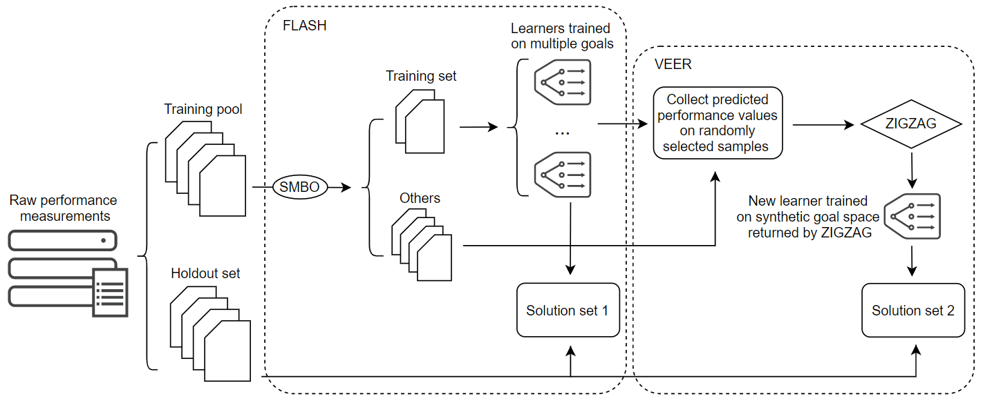

An overview of the framework using VEER is shown in Figure 3 (which also includes the experimental rig used in this paper). The component ZIGZAG, as illustrated in Figure 4, is the core heuristic used in VEER to generate the single-dimension objective space, and its implementation varies for different definitions of domination. In this paper, we choose to use the heuristic implemented with continuous domination because we believe it can better reflect and preserve the domination relationship among solutions in our setting: As one can observe from the two examples in Figure 4, when using binary domination, point is assigned a higher rank than point . However, if we only look at these two solutions, neither of them can dominate each other, thus, assigning them different ranks seems less reasonable. Such tricky situations can be avoided in the continuous domination scenario because points are ranked precisely according to their distance toward the "heaven" point (where both objectives are optimized).
for do
.append() // record the predicted performance values for the th objectives
while do
.remove()
.update() // record the current Pareto rank as depicted in Figure 4
FitModel()
// Fit a new model using PR as the dependent feature.
.predict()
//Those predicted to have lowest PR will be returned as final choice of configurations.
return
VEER uses CART as the final surrogate model motivated by effectiveness and interpretability considerations. As previously shown by FLASH, an optimizer model built with CART can achieve comparable and sometimes superior performance in multi-objective optimization as compared to GPM. One reason that CART scales better than GPM in data of larger dimensionality is that CART does not presume the "smoothness" of the data space: models like GPM make an assumption to the data space that configurations closer to each other have similar performance. Such assumption can usually be invalid because a seemingly small change in configuration options might actually represent a crucial shift in configuration strategy (i.e., the choice of data structure often has a substantial impact on the performance of a storage-oriented system). Our second consideration is interpretability. Gigerenzer pointed out that tree-structured models express great rationality and interpretability, making it easier for users to obtain actionable insights about the data Gigerenzer 2008. A recent survey about practitioners’ beliefs about visual explanations of defect prediction models also shows that CART is favoured by practitioners for its interpretability Jiarpakdee et al. 2021. The result of the survey reported that among 6 methods of offering visual explanations, CART is ranked as the 1st tier in terms of insightfulness and quality of the generated visual explanations.
Algorithm 3 offers details on VEER’s internal workings.
5 Research Questions
This section illustrates research questions and our strategy to address these questions.
To systematically evaluate its merits, we compared VEER with one of the most recent state-of-the-art configuration optimizer, FLASH. Moreover, to verify whether the model disagreement problem can be tamed via a simple and naive approach, we also implemented two variants of FLASH to serve as the baseline.
Our research questions are geared towards assessing the performance of VEER regarding 3 aspects: (a) effectiveness of configuration solutions generated from the model using VEER heuristic, (b) interpretability of VEER, and the (c) execution time of the model using VEER heuristic. More specifically, we ask the following research questions:
RQ1: Is there a model disagreement problem for multi-objective optimization of CSS?
Before doing anything else, we need to first motivate the investigation of this paper. In this research question, we ask whether the standard model-based method (FLASH) used in the multi-objective configuration problem results in conflicting suggestions on optimizing different objectives. To measure the level of such conflicts, we used the rank correlation measurement called Kendall’s test to assess whether learners trained on different objectives rank the candidate configurations in different orders.
RQ2: Is the disagreement problem “linearly solvable”?
All the technology proposed in this paper is superfluous if an existing alternate method can handle the problem of interpreting multi-objective optimization results. Therefore, we attempt to edit the default FLASH into two variants, using two different heuristic function to reduce the objective space: (a) the weighted sum equation and one single-output regression learner, or (b) a multi-output regression learner. The two benchmark methods are referred to as SingleWeight and MultiOut respectively. Our experiments will show that both methods have significant shortcomings.
RQ3: Can VEER resolve the model disagreement problem while maintaining on-par performance with benchmark methods?
Here, we test whether introduction of the VEER heuristic will compromise performance of the state-of-the-art optimizer . To measure that, we evaluate not only the quality of the returned solutions, but also the robustness of the model. Measurements used to evaluate the merits of VEER and other benchmark methods are elaborated in §6.3
RQ4: Can VEER reduce the execution time?
We explore other positive side effects brought by VEER. One of the most apparent improvements of VEER is that since multiple learners within the optimizer are replaced by a single learner, the model can now skip the step of computing domination sort across the whole holdout set, which is computationally very intense. To assess the extent of the improvement, we will record the execution time of VEER when applying it to the holdout set, and compare it with that of other benchmark methods.
6 Experimental Setup
To answer our research questions, our experiment compares the performance of configuration optimizers using VEER heuristic against those using alternative heuristics.
As depicted in Figure 3, all the configuration optimizers in our experiment will divide the configuration space into 2 sets: the training pool, and the holdout set (we split them 50% to 50%). Each optimizer sequentially samples along the training pool to add the selected next most informative configuration item into the training set (and this set is a subset of the training pool). The selected configurations and the corresponding performance measures are then used to train the machine learners within the optimizer. Then, the performance of each optimizer is evaluated using the holdout set. Apart from that, VEER has one additional step, which is to use the ZIGZAG process as illustrated in Figure 4 to train a hyper-space model using random samples chosen from the rest of the training pool. Note that, since this step does not require to access the actual performance measures of the additionally chosen samples , it will not increase the measurement cost in the real-world application. Finally, to assess the stability and reliability of our approach in a statistical manner, our experimentation will randomly choose 50% of the configuration space as the holdout set. To reduce the effect of the random seeds, the whole process is repeated for 100 times. For replication purposes, our code and datasets are on-line: https://github.com/anonymous12138/multiobj.
6.1 Data
To empirically evaluate the effectiveness of our approach, we use datasets collected from different configurable software systems. Each dataset contains the whole population of all valid configurations of that system and the performance measures of each configuration (by “all”, we mean all combinations given the selected configuration options). Table 2 describes the nature of each dataset. We selected the datasets based on the following criteria: (1) different sizes to examine the scalability and robustness, (2) different domains to improve external validity, and (3) different application domains (client-server and desktop) to cover different performance aspects (i.e., run time of compressing a video vs. run time to perform a set of actions on a database). Among all the datasets, SS-C and SS-F are datasets used in FLASH. Others (SS-A, SS-B, SS-D, SS-E, and SS-G to SS-K) are datasets recently collected by us. For datasets that are collected by us, we applied the following process: To reduce measurement noise, we executed all measurements in isolation (i.e., no other tasks are performed) on machines with minimal Debian 9 or Debian 10 installations and repeated each measurement 3–5 times. While the standard deviation of a performance measure exceeded , we repeated the measurement of the configuration.
6.2 Baselines
To assess our approach comprehensively, we included several SMBO methods as benchmark methods in out experiment. At first, we collected some existing open-source SMBO methods, such as FLASH Nair et al. 2018, HyperOpt Bergstra et al. 2013 (using TPE Bergstra et al. 2011 as surrogate models) and SMAC Hutter et al. 2011. Unfortunately, we found that both HyperOpt and SMAC do not support customized constraints on the search space. As illustrated in §3.2, such constraints are rather crucial as they filter out over 99% of invalid configurations Kaltenecker et al. 2020. Hence, we had to implement our own versions of the SingleWeight and MultiOut alogorithms described in §5. The implementation follows the SMBO framework as described in prior works Bergstra et al. 2011; Nair et al. 2018; Brochu et al. 2010, denoted as SingleWeight and MultiOut33 3 And the source code for that implementation can be found in the reproduction package mentioned in our abstract. The major difference among these benchmark methods is the output format of surrogate models (either single-output or multi-output) and option of using either weighted sum or non-dominated sorting to select the final solutions. The implementation of all benchmark methods is available in our online repository.
6.3 Performance Criteria
First of all, to assess effectiveness of our approach against benchmark models, we choose to measure the quality of the solutions set returned by each model. A solution set contains configurations that a model believes to have optimal performance among all configurations. Given the definitions of binary and continuous domination, a solution set can contain more than one configuration. To measure the quality of the solution set, this paper uses generational distance Van Veldhuizen 1999 (GD) as the indicator. GD computes the average distance between the solution set returned by a model and the actual optimal solution set. There are other indicator such as inverted generational distance Coello and Sierra 2004 (IGD) and hypervolume Huband et al. 2003 (HV). However, prior research suggests GD as a more suitable metric to uniformly reflect the overall quality of the solution set Agrawal et al. 2020. For example, if one intentionally adds very poor solutions into the solution set, IGD and HV cannot reflect the change in the overall quality of the new solution set.
Secondly, to assess the interpretability of a model, in this paper we are specifically assessing the level of disagreement among multiple learners within a multi-objective model. We argue that if interpretations extracted from different learners are conflicting or disagreeing with each other, the model will fail to provide stakeholders with unequivocal insights that are truly informatively or actionable. In that spirit, we use a rank correlation test, Kendall’s test Kendall 1948, to measure the extent of disagreements among learners built on different objectives. Kendall’s test is a non-parametric statistical test which can be used to measure the ordinal association between 2 lists of measured variables (in this paper, 2 objective values on the same configurations). According to the definition from Kendall correlation, we first categorize any pair of configurations by their performance measure into 2 kinds: discordant pairs and concordant pairs. Let and denote a pair of configurations, represented by the performance measures in objective and objective . This pair is concordant if the sorted order of and agrees: one configuration has better performance than the other in both objectives44 4 We define a concordant pair in tasks of more than 2 objectives in a similar manner: one configuration has better performance than the other in all objectives. This is not originally defined by Kendall, but we believe it is a proper extension.. Otherwise, the pair is discordant. After that we compute the Kendall coefficient using the following equation:
| (4) |
where P is the number of concordant pairs, Q the number of discordant pairs. In general, the Kendall correlation is high when the 2 variables are ranked similarly, and the correlation is low when the 2 variables are ranked differently. More specifically in our case study, a positive coefficient means a relatively similar ordering among different objectives, which indicates less disagreement among different learners in a multi-objective model; A coefficient near 0 means the 2 lists of ranks assigned by different learners have no correlation at all; A negative coefficient means the learners rank configurations in somehow opposite order.
Finally, to assess computational complexity of our approach, we measure the execution time of applying each model on the holdout data to generate a solution set. All the above analyses and measurements were executed on a 64-bit Windows 10 machine with a 2.2 GHz 4-core Intel Core i5 processor and 8 GB of RAM.
6.4 Statistical Analysis
To make comparisons among all algorithms on a single project, we use a non-parametric significance test and a non-parametric effect size. Specifically, we use the Scott-Knott test Mittas and Angelis 2012 that sorts the list of treatments (in this paper, VEER and baselines) by their median scores. After the sorting, it then splits the list into two sub-lists. The objective for such a split is to maximize the expected value of differences in the observed performances before and after division Xia et al. 2018:
| (5) |
where means the size of list . The Scott-Knott test assigns ranks to each result set; the higher the rank, the better the result. Two results will be ranked the same if the difference between the distributions is not significant. In this expression, Cliff’s Delta estimates the probability that a value in list is greater than a value in list , minus the reverse probability Macbeth et al. 2011. A division passes this hypothesis test if it is not a “small” effect (). This hypothesis test and its effect size are supported by Hess and Kromery Hess and Kromrey 2004.
7 Results
This section provides experiment results that answer the research questions (RQs) previously discussed.
7.1 RQ1
Is there a model disagreement problem for multi-objective optimization of CSS?
Table 3 checks for the existence of this problem by showing the rank correlation of FLASH, which is measured by Kendall’s coefficient. As shown in Table 3, there are a few systems where the rank correlation is relatively high (SS-I and SS-K). This could be because the objectives in those systems are not so conflicting. In such cases, feature interactions learned from different learners are likely to be homogeneous since essentially these learners can substitute each other without harming the model performance. On the other hand, for most of the case studies in this paper, we do observe that configurations are ranked in a rather opposite way by learners trained on different objectives.
In summary, we answer RQ1 as follows:
| FLASH (Default) | SingleWeight | MultiOut | VEER | |
|---|---|---|---|---|
| SS-A | 0.47 | 1.00 | 0.82 | 1.00 |
| SS-B | 0.16 | 1.00 | 0.13 | 1.00 |
| SS-C | 0.60 | 1.00 | 0.65 | 1.00 |
| SS-D | -0.17 | 1.00 | -0.07 | 1.00 |
| SS-E | -0.56 | 1.00 | -0.54 | 1.00 |
| SS-F | -0.30 | 1.00 | -0.30 | 1.00 |
| SS-G | -0.47 | 1.00 | -0.51 | 1.00 |
| SS-H | -0.69 | 1.00 | -0.69 | 1.00 |
| SS-I | 0.73 | 1.00 | 0.73 | 1.00 |
| SS-J | -0.08 | 1.00 | -0.17 | 1.00 |
| SS-K | 0.87 | 1.00 | 0.88 | 1.00 |
7.2 RQ2
Is the disagreement problem “linearly solvable”?
This section compares the results of FLASH (which works on each objective separately) to MultiOut and SingleWeight (which work on some linear combinations of the objectives).
For MultiOut, we show in Table 3 that we can increase the rank correlation by replacing the multiple single-output CART learners with a single multi-output CART learner. This could be a good sign implying that in some cases FLASH can be easily improved in the model disagreement problem via making a small mutation on its original implementation. However, such improvement does have its upper bound, given the disagreement still exists pervasively among all datasets.
As for SingleWeight, because we beforehand transformed multi-objective space into a single objective via a weighted sum function, the optimizer now requires one surrogate model. This totally resolved the disagreement problem by reducing the arity of output. However, as later reported in Table 4, this approach can sometimes compromise the performance significantly. We conjecture that it could be because the optimal solutions are not uniformly distributed or the optimal solutions reside in a non-convex region which leads the weighted sum approach to fail.
In summary, we answer RQ2 as follows:
| FLASH (Default) | SingleWeight | MultiOut | VEER | |
|---|---|---|---|---|
| SS-A | 0.007 | 0.011 | 0.014 | 0.013 |
| SS-B | 0.125 | 0.171 | 0.100 | 0.119 |
| SS-C | 0.020 | 0.021 | 0.019 | 0.022 |
| SS-D | 0.060 | 0.059 | 0.061 | 0.058 |
| SS-E | 0.131 | 0.135 | 0.144 | 0.136 |
| SS-F | 0.098 | 0.082 | 0.113 | 0.113 |
| SS-G | 0.014 | 0.296 | 0.016 | 0.014 |
| SS-H | 0.013 | 0.013 | 0.016 | 0.013 |
| SS-I | 0.034 | 0.038 | 0.034 | 0.042 |
| SS-J | 0.386 | 0.437 | 0.384 | 0.362 |
| SS-K | 0.299 | 0.306 | 0.304 | 0.298 |

7.3 RQ3
Can VEER resolve the model disagreement problem while maintaining on-par performance with benchmark methods?
First of all, we need to clarify that we will not use the rank correlation as the major indicator to evaluate the merit of our approach. The reason is, when the model used to generate the solution set is a single-output learner, there is naturally no disagreement at all, which always guarantees a perfect correlation (Kendall’s coefficient = 1). This result is totally to be expected by us since VEER is designed purposefully to resolve the disagreement problem.
Therefore, we need to evaluate whether VEER compromises the performance as compared to FLASH. In Table 4, we report the generational distance (GD) of solution sets provided by each optimizer. We used a non-parametric effect size test to determine if the difference between the two performance measures is statistically significant. As shown by the table, in most cases VEER can achieve comparable performance. We note in Figure 5 that VEER in some cases has a slightly larger variance than other methods. Specifically, in four cases out of eleven (SS-B, SS-C, SS-F, SS-I), VEER has a larger inter-quartile (IQR) than FLASH. This was actually a pre-experimental expectation since VEER is a patch on FLASH (so VEER gets all the variance of FLASH, plus some extra "wriggle" due to its own learning process). It is also noteworthy that in the majority datasets (SS-A, SS-C, SS-D, SS-G, SS-H, SS-I, SS-K), the inter-quartile range of VEER was very small (less than ). Lastly, we note that while that IQR is larger, the significance of that larger size does not effect our argument (as supported by the statistical tests in §6.4.)
In summary, we answer RQ3 as follows:

7.4 RQ4
Can VEER reduce the execution time?
While executing VEER during the experimentation, one of the most obvious bonuses is that VEER runs much faster than prior methods when applied to the holdout set. As shown in Figure 6, the average execution time using VEER when applied to the holdout set is much faster than that of other benchmark methods. The model can be up to 1000+ times faster than other benchmarks when applied on the largest dataset. Note that we also observe a larger variance in runtime when the size of datasets increases. This is because the runtime is also hugely influenced by the size of the returned solutions set: when there are more non-dominated solutions in the holdout set, the time till the termination of the non-domination sort will increase proportionally. VEER does not suffer from such complexity given its design of "compressing" multi-objective space into a single dimension.
In summary, we answer RQ4 as follows:
8 Discussion
In this section we discuss what makes VEER novel and more useful than prior methods in optimizing multi-objective configuration.
Final interpretations: In the domain of multi-objective optimization, final solutions are yielded by processing non-dominated sorting first. However, this part is non-parametric and cannot be used to extract interpretation. Therefore, traditional SMBO optimizers are only capable of providing preliminary interpretations from single-objective models. The same attribute is also reflected on Clafer, the configuration visualizer: Clafer helps practitioners understand the commonalities and variants among different configuration solutions on the Pareto frontier. However, such instance-based visualization cannot yield generalizable rules on how to optimize multiple goals. VEER, on contrary, provides final rule-based interpretations about how to optimize a configuration in general.
Fast: Non-dominated sorting is a computation-intensive step with an optimizer. VEER replaces it with the hyper-space model that mimics the behavior of the non-dominating sorting procedure. By directly learning the relationship between the non-dominated ranks and the independent variables (configuration options), VEER can achieve significantly (up to in the largest system) faster execution time.
Adjustable: In addition to the merits above, VEER can also incorporate with the preference-based approach by simply adjusting the distance calculation function insides ZIGZAG. As shown in Figure 7, by customizing the preference weights (e.g., means optimizing one objective is twice as important as optimizing the other one), VEER can generate solutions that reflect such user preferences.
Uncompromising: Our approach cannot be generalizable to all configurable software systems: when two objectives are competing (with strong negative correlation), VEER is doomed to fail since a configuration that optimizes one objective will inevitably compromise the other one by the same extent. However, we show that this is not the case in datasets explored so far. In fact, VEER can generate disagreement-free interpretations without compromising the performance in most cases; In others, VEER inevitably suffers from greater variances.
9 Threats to validity
Given the complexity of our experiments in 11 real-world configurable software systems, many factors can threaten the validity of our results.
Internal Validity. First of all, the multi-objective optimizer learns from benchmark measurements that we collected from various configurable systems. While we have rejected measurements with relatively high variance, it remains possible that some measurements are incorrect, which can bias the learning procedure of the optimizer and may result in worse solution sets.
Secondly, we measure the level of model disagreement using a rank correlation test, namely Kendall’s test. One shortcoming of this test is that it has to be performed on ranks assigned to the same set of variables, which forces us to compute the correlation on the whole population (since optimal solutions defined by different objectives are hardly the same). As is well-known, it is actually the optimal (non-dominated) solution set that an optimizer cares about, and the very majority of the whole population are only sub-optimal solutions. Therefore, it could be a possible case that there is actually little disagreement within the optimal solutions but much disagreement among the sub-optimal space.
External Validity. While we believe our findings is generalizable as supported by the experimentation result, this does not guarantee the model to be automatically scalable to systems with larger spaces and dimensionalities. However, to increase the external validity of our study, we did intentionally choose datasets from various sizes, dimensions, and application domains.
Secondly, we select CART as the embedded surrogate model because prior research has shown that CART is capable to achieve good performance and has great interpretability with feature interactions being presented as decision conditions within the tree Nair et al. 2018. Another consideration is that since we use FLASH, one of the most recent state-of-the-art optimization models, as the benchmark method, we would prefer to control variables within the experiment so that our comparison is sufficiently "fair". That said, it is possible that other white-box machine learners (e.g., logistic regression, Naive Bayes) can achieve superior performance than CART while we have not explored yet. However, this paper is centered around assessing the feasibility of our proposed method used to improve Pareto-based optimization. Our current experiment results suffice to illustrate the effectiveness of our work.
10 Conclusion
We have shown that model disagreement is rampant in the standard case studies used to assess multi-objective configuration problems. As stated in our introduction, the current literature has surprisingly little on this topic. Hence we are concerned that model disagreement may be a long-standing, but previously under-explored, problem.
To better address this problem, we have proposed a confusion-free multi-objective configuration optimizer, VEER, which is built on top of a state-of-the-art sequential model-based optimizer FLASH. We have shown that VEER has not only inherited many merits of FLASH (good performance and low training cost), but also resolved the potential model disagreement problem. We have demonstrated the effectiveness of VEER in resolving model disagreement while maintaining on-par quality for the configuration solutions.
To do this, first, we investigated the existence of model disagreement problem in cases studied in this paper, where the interpretations returned by FLASH can sometimes be conflicting, as indicated by the rank correlation.
Second, we demonstrated that VEER can enhance the shortcoming of FLASH. VEER is capable of mapping an N-dimensional objective space (in this paper, is 2 and 3) onto a single-dimensional space without information loss of the domination relationship. Since the synthetic single-dimensional objective space can be learned by just one machine learner, the model disagreement problem collapses in itself.
Finally, we have shown that VEER can achieve on-par performance compared to the original FLASH model, indicating no information loss during the procedure.
Another bonus of VEER is that by simplifying the objective space, the execution time of applying the optimizer model during the testing (or deployment) time has been dramatically reduced (1,000 times at most). It is also noteworthy that since the computational cost of VEER is also relatively small compared to that of an optimizer, the overhead of adding VEER on top of any model-based optimizer should be trivial.
Regarding future work, we will invest our effort in addressing open issues described in §9. Beyond that, we believe VEER can be not only applicable in configuration optimization tasks, but also hyper-parameter tasks from machine learning techniques as described in the FLASH paper Nair et al. 2018. Moreover, there exists an increasing demand for commissions such as auto-generated code (from chatGPT or Copilot, etc.) to the local domain. Tools like VEER might be useful for tuning the choice points inside that code (e.g., given a genetic -th nearest neighbor code snippet from chatGPT, designers could use VEER to decide what is the best setting for .
Acknowledgements
This work was partially funded by a research grant from the Laboratory for Analytical Sciences, North Carolina State University. Apel’s work has been funded by the German Research Foundation (AP 206/11 and Grant 389792660 as part of TRR 248 – CPEC. Siegmunds work has been supported by the Federal Ministry of Education and Research of Germany and by the Sächsische Staatsministerium für Wissenschaft Kultur und Tourismus in the program Center of Excellence for AI-research "Center for Scalable Data Analytics and Artificial Intelligence Dresden/Leipzig", project identification number: ScaDS.AI, and by the German Research Foundation (SI 2171/2-2).
Declarations
Funding and Conflicts of interests
Apart from the funding acknowledged above, this work does not have any other conflicts of interests.
References
- Agrawal et al. (2020) Agrawal A, Menzies T, Minku LL, Wagner M, Yu Z (2020) Better software analytics via “duo”: Data mining algorithms using/used-by optimizers. Empirical Software Engineering 25(3):2099–2136
- Antkiewicz et al. (2013) Antkiewicz M, Bąk K, Murashkin A, Olaechea R, Liang JH, Czarnecki K (2013) Clafer tools for product line engineering. In: Proceedings of the 17th international software product line conference co-located workshops, pp 130–135
- Bergstra et al. (2011) Bergstra J, Bardenet R, Bengio Y, Kégl B (2011) Algorithms for hyper-parameter optimization. Advances in neural information processing systems 24
- Bergstra et al. (2013) Bergstra J, Yamins D, Cox DD, et al. (2013) Hyperopt: A python library for optimizing the hyperparameters of machine learning algorithms. In: Proceedings of the 12th Python in science conference, Citeseer, vol 13, p 20
- Brochu et al. (2010) Brochu E, Cora VM, De Freitas N (2010) A tutorial on bayesian optimization of expensive cost functions, with application to active user modeling and hierarchical reinforcement learning. arXiv preprint arXiv:10122599
- Chen et al. (2018a) Chen D, Fu W, Krishna R, Menzies T (2018a) Applications of psychological science for actionable analytics. In: Proceedings of the 2018 26th ACM Joint Meeting on European Software Engineering Conference and Symposium on the Foundations of Software Engineering, pp 456–467
- Chen et al. (2018b) Chen J, Nair V, Krishna R, Menzies T (2018b) "sampling" as a baseline optimizer for search-based software engineering. IEEE Transactions on Software Engineering (pre-print) pp 1–1
- Coello and Sierra (2004) Coello CAC, Sierra MR (2004) A study of the parallelization of a coevolutionary multi-objective evolutionary algorithm. In: Mexican international conference on artificial intelligence, Springer, pp 688–697
- Deb et al. (2002) Deb K, Pratap A, Agarwal S, Meyarivan T (2002) A fast and elitist multiobjective genetic algorithm: Nsga-ii. IEEE transactions on evolutionary computation 6(2):182–197
- Devanbu et al. (2016) Devanbu P, Zimmermann T, Bird C (2016) Belief & evidence in empirical software engineering. In: 2016 IEEE/ACM 38th International Conference on Software Engineering (ICSE), IEEE, pp 108–119
- Gigerenzer (2008) Gigerenzer G (2008) Why heuristics work. Perspectives on psychological science 3(1):20–29
- Golovin et al. (2017) Golovin D, Solnik B, Moitra S, Kochanski G, Karro J, Sculley D (2017) Google vizier: A service for black-box optimization. In: Proceedings of the 23rd ACM SIGKDD international conference on knowledge discovery and data mining, pp 1487–1495
- Guo et al. (2018) Guo J, Yang D, Siegmund N, Apel S, Sarkar A, Valov P, Czarnecki K, Wasowski A, Yu H (2018) Data-Efficient Performance Learning for Configurable Systems. Empirical Software Engineering (EMSE) 23(3):1826–1867
- Herodotou et al. (2011) Herodotou H, Lim H, Luo G, Borisov N, Dong L, Cetin FB, Babu S (2011) Starfish: A self-tuning system for big data analytics. In: Conference on Innovative Data Systems Research
- Hess and Kromrey (2004) Hess MR, Kromrey JD (2004) Robust confidence intervals for effect sizes: A comparative study of cohen’sd and cliff’s delta under non-normality and heterogeneous variances. In: annual meeting of the American Educational Research Association, pp 1–30
- Holland (1992) Holland JH (1992) Genetic algorithms. Scientific american 267(1):66–73
- Huband et al. (2003) Huband S, Hingston P, While L, Barone L (2003) An evolution strategy with probabilistic mutation for multi-objective optimisation. In: The 2003 Congress on Evolutionary Computation, 2003. CEC’03., IEEE, vol 4, pp 2284–2291
- Hutter et al. (2011) Hutter F, Hoos HH, Leyton-Brown K (2011) Sequential model-based optimization for general algorithm configuration. In: 5th LION
- Jiarpakdee et al. (2021) Jiarpakdee J, Tantithamthavorn C, Grundy J (2021) Practitioners’ perceptions of the goals and visual explanations of defect prediction models. arXiv preprint arXiv:210212007
- Kaltenecker et al. (2020) Kaltenecker C, Grebhahn A, Siegmund N, Apel S (2020) The interplay of sampling and machine learning for software performance prediction. IEEE Software 37(4):58–66
- Kendall (1948) Kendall MG (1948) Rank correlation methods.
- Kolesnikov et al. (2019) Kolesnikov S, Siegmund N, Kästner C, Grebhahn A, Apel S (2019) Tradeoffs in modeling performance of highly configurable software systems. Software & Systems Modeling 18(3):2265–2283
- Laumanns et al. (2002) Laumanns M, Thiele L, Deb K, Zitzler E (2002) Combining convergence and diversity in evolutionary multiobjective optimization. Evolutionary computation
- Macbeth et al. (2011) Macbeth G, Razumiejczyk E, Ledesma RD (2011) Cliff’s delta calculator: A non-parametric effect size program for two groups of observations. Universitas Psychologica 10(2):545–555
- Mittas and Angelis (2012) Mittas N, Angelis L (2012) Ranking and clustering software cost estimation models through a multiple comparisons algorithm. IEEE Transactions on software engineering 39(4):537–551
- Nair et al. (2017) Nair V, Menzies T, Siegmund N, Apel S (2017) Using bad learners to find good configurations. In: Proceedings of the 2017 11th Joint Meeting on Foundations of Software Engineering, pp 257–267
- Nair et al. (2018) Nair V, Yu Z, Menzies T, Siegmund N, Apel S (2018) Finding faster configurations using flash. IEEE Transactions on Software Engineering 46(7):794–811
- Sarkar et al. (2015) Sarkar A, Guo J, Siegmund N, Apel S, Czarnecki K (2015) Cost-efficient sampling for performance prediction of configurable systems (t). In: 2015 30th IEEE/ACM International Conference on Automated Software Engineering (ASE), IEEE, pp 342–352
- Sawyer (2011) Sawyer R (2011) Bi’s impact on analyses and decision making depends on the development of less complex applications. IJBIR 2:52–63, DOI 10.4018/IJBIR.2011070104
- Shrikanth and Menzies (2020) Shrikanth N, Menzies T (2020) Assessing practitioner beliefs about software defect prediction. In: 2020 IEEE/ACM 42nd International Conference on Software Engineering: Software Engineering in Practice (ICSE-SEIP), IEEE, pp 182–190
- Siegmund et al. (2015) Siegmund N, Grebhahn A, Apel S, Kästner C (2015) Performance-Influence Models for Highly Configurable Systems. In: Proceedings of the Joint Meeting on Foundations of Software Engineering (ESEC/FSE), ACM, pp 284–294
- Snoek et al. (2012) Snoek J, Larochelle H, Adams R (2012) Practical bayesian optimization of machine learning algorithms. In: NIPS - Volume 2
- Song and Chan (2015) Song W, Chan FT (2015) Multi-objective configuration optimization for product-extension service. Journal of Manufacturing Systems 37:113–125
- Tan and Chan (2016) Tan SY, Chan T (2016) Defining and conceptualizing actionable insight: a conceptual framework for decision-centric analytics. arXiv preprint arXiv:160603510
- Tu et al. (2021) Tu H, Papadimitriou G, Kiran M, Wang C, Mandal A, Deelman E, Menzies T (2021) Mining workflows for anomalous data transfers. In: 2021 IEEE/ACM 18th International Conference on Mining Software Repositories (MSR), pp 1–12, DOI 10.1109/MSR52588.2021.00013
- Van Aken et al. (2017) Van Aken D, Pavlo A, Gordon GJ, Zhang B (2017) Automatic database management system tuning through large-scale machine learning. In: International Conference on Management of Data, ACM
- Van Veldhuizen (1999) Van Veldhuizen DA (1999) Multiobjective evolutionary algorithms: classifications, analyses, and new innovations. Tech. rep., AIR FORCE INST OF TECH WRIGHT-PATTERSONAFB OH SCHOOL OF ENGINEERING
- Xia et al. (2018) Xia T, Krishna R, Chen J, Mathew G, Shen X, Menzies T (2018) Hyperparameter optimization for effort estimation. arXiv preprint arXiv:180500336
- Xu et al. (2015) Xu T, Jin L, Fan X, Zhou Y, Pasupathy S, Talwadker R (2015) Hey, you have given me too many knobs!: understanding and dealing with over-designed configuration in system software. In: Foundations of Software Engineering
- Zhang and Li (2007) Zhang Q, Li H (2007) Moea/d: A multiobjective evolutionary algorithm based on decomposition. IEEE Transactions on evolutionary computation 11(6):712–731
- Zhu et al. (2017) Zhu H, Jin J, Tan C, Pan F, Zeng Y, Li H, Gai K (2017) Optimized cost per click in taobao display advertising. arXiv preprint
- Zitzler et al. (2001) Zitzler E, Laumanns M, Thiele L (2001) Spea2: Improving the strength pareto evolutionary algorithm. TIK-report 103
- Zuluaga et al. (2016) Zuluaga M, Krause A, Püschel M (2016) -pal: an active learning approach to the multi-objective optimization problem. The Journal of Machine Learning Research 17(1):3619–3650