Superconducting on-chip spectrometer for mesoscopic quantum systems
Abstract
Spectroscopy is a powerful tool to probe physical, chemical, and biological systems. Recent advances in microfabrication have introduced novel, intriguing mesoscopic quantum systems including superconductor-semiconductor hybrid devices and topologically non-trivial electric circuits. A sensitive, general purpose spectrometer to probe the energy levels of these systems is lacking. We propose an on-chip absorption spectrometer functioning well into the millimeter wave band which is based on a voltage-biased superconducting quantum interference device. We demonstrate the capabilities of the spectrometer by coupling it to a variety of superconducting systems, probing phenomena such as quasiparticle and plasma excitations. We perform spectroscopy of a microscopic tunable non-linear resonator in the 40-50 GHz range and measure transitions to highly excited states. The Josephson junction spectrometer, with outstanding frequency range, sensitivity, and coupling strength will enable new experiments in linear and non-linear spectroscopy of novel mesoscopic systems.
I Introduction
Soon after the theoretical prediction of the Josephson effect, researchers directly measured microwave emission from a superconducting tunnel junction Yanson et al. 1965a and demonstrated that such junctions can also be used as detectors of external radiation Grimes et al. 1966. Silver and Zimmerman were the first to combine the emission and detection capabilities of Josephson junctions to make an integrated absorption spectrometer Silver and Zimmerman 1967. Using a voltage-biased superconducting point contact coated in powdered cobalt, they measured the nuclear magnetic resonance response of Co59 at in the point-contact current-voltage characteristic. Deaver extended the technique to higher frequencies with a niobium point contact coated with a resonant absorber, measuring features in the current-voltage characteristic at corresponding to the absorber frequency Deaver 1974.
Despite these early efforts coupling Josephson junctions to bulk samples, there have been few applications of the technique for spectroscopy of mesoscopic systems, artificial quantum coherent structures. Using specialized circuits in each case, researchers have measured Josephson plasma modes Kleinsasser et al. 2005, resonances in microresonators Edstam and Olsson 1994; Holst et al. 1994, the energy levels of Cooper pair transistors Lindell et al. 2003a; Billangeon et al. 2007; Basset et al. 2012, spin-wave resonances Petković et al. 2009, and Andreev bound states Bretheau et al. 2013; van Woerkom et al. 2017. Although Josephson junction based absorption spectroscopy has the potential to access a frequency range spanning to with unprecedented sensitivity, progress has been impeded by several technical challenges. The bandwidth is strongly limited by junction capacitance, parasitic electromagnetic modes are prevalent, and the low-frequency region is dominated by artifacts from the biasing circuit. We overcome these difficulties, implementing a uniform coupling scheme, variable output power, and reduction of background resonances, in order to realize a general-purpose spectrometer for mesoscopic systems.
The Josephson relations Josephson 1962 imply that a superconducting tunnel junction biased at a DC voltage is comparable to an alternating current source of frequency and amplitude , the critical current. The oscillating Josephson currents may excite resonances of the junction’s electromagnetic environment, resulting in a change in the DC current which can be explained by energy conservation Eck et al. 1964; Fiske 1964; Yanson et al. 1965b; Yanson et al. 1965a. The power dissipated in the junction’s electromagnetic environment by the high-frequency currents must be balanced by the DC power supplied by the source to maintain the voltage Werthamer 1966; Werthamer and Shapiro 1967; Likharev 1986.
In a microscopic quantum view, the back and forth tunneling of Cooper pairs in a voltage-biased junction is accompanied by the emission and re-absorption of photons at an energy Ingold et al. 1994; Bretheau et al. 2014. The junction’s electromagnetic environment may include a generic device-under-test (DUT) with a well-defined photon absorption peak, such as a two-level system with an energy difference between ground and excited states [Fig. 1(a)]. At resonance, , the DUT can absorb photons emitted by the junction, with one Cooper pair tunneling per absorbed photon. Relaxation from excited states of the DUT will result in a steady-state photon absorption rate which must be matched by a DC Cooper-pair tunneling current . Because of the large voltage-to-frequency conversion ratio, , where is the magnetic flux quantum, the DC current-voltage characteristic of the Josephson junction (JJ) corresponds to the millimeter wave absorption spectrum of the DUT and its environment.
For a Josephson spectrometer based on a symmetric superconducting quantum interference device (SQUID) Clarke and Braginski 2004, as sketched in Fig. 1(b), consisting of two JJs (boxed crosses) in a superconducting loop, the direction of the emitted radiation will depend on the total static magnetic flux threading the loop. When the SQUID inductance is negligible, is equal to the applied magnetic flux. The phase difference between the two JJs in the loop is given by the total reduced flux, . When the total flux is a multiple of the flux quantum, and there is non-zero bias voltage , the junctions are in phase () and an oscillating current of amplitude and frequency flows in the biasing leads (common mode). On the contrary when the SQUID is frustrated, with the total flux which is a multiple of half a flux-quantum, the junctions are out-of-phase (). An oscillating current of amplitude circulates in the superconducting loop, generating an oscillating out-of-plane magnetic field (differential mode).
For a DUT coupled to the electromagnetic field above the spectrometer loop, only the differential mode can excite transitions. At few photons are coupled to the DUT but many propagate in the common mode along the biasing leads, Fig. 1(b) (blue schematic). These photons may excite spurious electromagnetic modes in the biasing circuit, especially at lower frequencies where the impedance of the external environment may be large. Therefore there will be significant DC current in the spectrometer current-voltage characteristic at low voltages and a negligible absorption peak at the DUT resonant voltage , as shown in the schematic Fig. 1(c) (blue, ).
Near half a flux-quantum many photons couple to the DUT and few excite the common mode, Fig. 1(b) (red schematic), resulting in a current-voltage characteristic with a large DUT absorption peak and little background signal at low voltages, Fig. 1(c) (red, ).
The magnetic flux simultaneously tunes the power delivered to the DUT by the spectrometer and decouples the spectrometer from the external, or “off-chip,” electromagnetic environment. In the low power or linear spectroscopy regime, where , only the first few excited states of the DUT are probed. For the power delivered to the DUT is large enough to access the non-linear spectroscopy regime and probe excited states. Changes in the shape of an absorption peak with increasing power reveals the anharmonicities typically found in mesoscopic systems.
II Spectrometer implementation
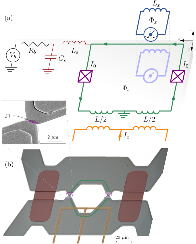
The advantages of using a frustrated SQUID as a Josephson spectrometer is that coupling to parasitic modes is reduced, the bandwidth is enhanced, and the power output is tunable. Excitation of a general mesoscopic system can be implemented by coupling it to the spectrometer loop inductance via the generated magnetic field [Fig. 1], the magnetic flux [Fig. 2], galvanically by inserting the DUT in the loop [Fig. 4], or capacitively with a parallel connection. The coupling scheme can be adapted to the DUT, with low impedance mesoscopic devices such as superconducting ones suited for flux or galvanic coupling, whereas higher impedance devices, including spins or semiconductor crystals, better suited for capacitive coupling.
We describe in detail below a Josephson spectrometer with inductive coupling which allows for strong driving while allowing the DUT to be located on a separate chip. A simplified electrical schematic for the Josephson spectrometer, including voltage and flux biasing circuits, is shown in Fig. 2(a). The DUT, indicated as a two-level system, is embedded in a superconducting loop of geometric inductance enclosing a total flux and positioned above the spectrometer SQUID (purple boxed crosses in green superconducting loop) so as to couple only to the differential mode. The total flux threading the DUT loop will differ from the applied flux when screening of magnetic fields must be taken into account.
Due to the inductive coupling scheme the DUT does not need to be located on the same chip as the spectrometer, as shown in Appendix B, and the mutual coupling coefficient will depend on the relative positions of the DUT and spectrometer [Appendix C]. The maximum amplitude of the oscillating magnetic flux generated by the spectrometer is , where is the geometric inductance of the spectrometer loop. For a DUT coupled to the spectrometer differential mode, the coupling energy can be approximated as Dmytruk et al. 2021. The Josephson energy of a spectrometer junction is and is the average phase difference across the spectrometer. The phase difference across the DUT, , is equal to the total reduced flux .
An external coil (not-shown) combined with an on-chip gradiometric inductor (orange), with control current , allows independent flux biasing of both spectrometer () and DUT (). The gradiometric line is designed to avoid inducing flux in the spectrometer loop but a calibration procedure is necessary to relate the control currents to the total flux in each loop, as well as to account for non-linear screening [Appendix E]. Passive filtering, both on-chip () and off-chip, help reduce spurious electromagnetic resonances in the spectrum. The Josephson junctions comprising the spectrometer as well as the surrounding circuit, including filtering and bias, Fig. 2(b), is fabricated using standard microlithography techniques [Appendix A].

We first demonstrate operation of a spectrometer in the absence of a DUT, Fig. 3. Current-voltage characteristics are plotted for two spectrometer phases in Fig. 3(a). The phase-dependence of the supercurrent branch is as expected for a SQUID, Fig. 1(b), with a maximum at and minimum at . The non-zero switching current minimum is due to a small difference in the size of the two junctions comprising the SQUID. In these and subsequent current-voltage characteristics, discontinuous switching (dashed lines) may occur at the top of peaks, including the supercurrent branch at zero voltage, due to the load line given by the bias resistor [Fig. 2(b)]. Quasiparticle conduction results in a sharp increase in current at knee voltages , corresponding to a typical thin-film aluminum value for , the superconducting energy gap.
Near zero flux bias () and , corresponding to , there is an extraneous absorption peak, highlighted in Fig. 3(a, inset), which can be identified as an electromagnetic resonance of the series biasing circuit. Biasing at greatly reduces the height of this peak and results in a virtually flat background over the whole frequency range, as shown in the log scale sensitivity plot, Fig. 3(b).
The intrinsic spectrometer sensitivity is defined as the minimum DUT absorption rate which exceeds the background noise in a given measurement bandwidth. As the background noise increases it is more difficult to identify the current signal due to absorption by the DUT. The intrinsic current noise of a Josephson tunnel junction, similarly to a photodetector, is given by the shot noise spectral density , where is the DC background current. In order to improve sensitivity the dark count rate must be minimized, motivating a spectrometer design and fabrication process which results in small background currents. For Fig. 3(b) the dark current of the spectrometer was measured with a long averaging time and converted to a shot-noise sensitivity in a bandwidth. The intrinsic spectrometer sensitivity away from the extraneous peak is approximately , corresponding to noise equivalent power (NEP) of at . Sensitivity in the range is better at phase bias due to the reduced height of the spurious resonance. The intrinsic sensitivity compares favorably to existing spectrometers [Table 1], but the total sensitivity will be worse due to extrinsic factors such as current noise in the biasing circuit. The external noise can be reduced by improved filtering, and the signal can be improved by cryogenic amplification and a photo-detector type current measurement circuit Hobbs 2001; Curry et al. 2019.
The full phase dependence of the spectrometer is shown in the spectral map Fig. 3(c), where the current, proportional to the absorption rate , is plotted in color scale as a function of bias voltage (left axis) as well as frequency (right axis). The current-voltage curves for and are indicated by dashed lines. Adjusting the spectrometer phase not only changes the DC supercurrent, but also the power output of the high-frequency Josephson oscillations at non-zero voltage. Since there is no DUT the spurious resonance at () is the only remarkable feature. The current peak due to absorption by this mode evolves in-phase with the supercurrent peak at , with a maximum at and minimum at . Such phase dependence for an absorption peak is a signature that the resonance couples to the common mode and is in series with the spectrometer. At , the background is flat and the spectrometer is decoupled from this series resonance.
Unlike with previous realizations of Josephson spectrometers, the inductive nature of the coupling scheme used here ensures that the coupling strength at flux bias is uniform and independent of frequency up to an intrinsic “loop resonance” Zimmerman and Sullivan 1977; Zappe and Landman 1978; Song and Hurrell 1979; Tuckerman and Magerlein 1980. The loop mode is a lumped element resonance of the spectrometer circuit Fig. 2(b) with angular frequency where is the loop inductance, proportional to the loop perimeter, and is the capacitance of a single junction. The coupling to the loop mode is maximal at , resulting in an absorption peak which is 180° out of phase with the supercurrent peak and any series resonant modes. Above the loop resonance frequency, the coupling to the DUT decreases rapidly as .
For the spectrometer shown in Fig. 3 the loop mode frequency was designed to exceed and so it is not visible in the map Fig. 3(c). Appendix F describes a spectrometer with a larger perimeter for which the loop mode is present in measurements.


To demonstrate how Josephson spectroscopy can be useful in probing mesoscopic systems, in Fig. 4 we show the measured quasiparticle absorption spectrum of a short superconducting wire and the plasma resonance of a large Josephson junction.
In Fig. 4(a), quasiparticles are excited in the superconducting loop of the spectrometer when it emits photons of energy greater than , occurring for bias voltage . This absorption is described by the Mattis-Bardeen theory for the frequency-dependent conductivity of superconductors with a BCS density of states Mattis and Bardeen 1958. A numerical fit to the theory (dash-dotted line) closely follows the measured current rise at . The additional current relative to the Mattis-Bardeen prediction above is due to the spectrometer loop mode at and can be accounted for with an additional lumped-element model (full fit, orange dashed line). The fit parameters, including the normal state resistance () and the loop mode frequency (), coincide with estimated values extracted from the junction capacitance (approximately ) and loop geometry (approximate width , perimeter , inductance ) Khapaev and Kupriyanov 2015. The two additional narrow peaks are attributed to inadvertent parasitic resonances Griesmar 2018. For unconventional superconductors, similar Josephson spectroscopy measurements could determine the form of the quasiparticle density of states and reveal the symmetry of the order parameter Sauls et al. 2015.
In Fig. 4(b), another Josephson spectrometer (inset, black) is galvanically coupled to a large Josephson junction (inset, red) embedded in the spectrometer loop. The area of the large junction is whereas each junction of the spectrometer has area Griesmar 2018. The spectral map shows Fraunhofer like absorption bands as a function of , the reduced flux which threads the large junction. Although the applied flux is nominally oriented out-of-plane, a small fraction links the junction as stray in-plane flux due to misalignment and field distortion via the Meissner effect. The Josephson plasma resonance, which disperses as , is identified as and fit with a plasma frequency (red dashed line), consistent with the estimated value, . A possible second harmonic of this mode as well as additional features in between and can be distinguished Griesmar 2018. The narrow repetitive feature at low voltage corresponds to the flux modulation of the spectrometer critical current. Previously, plasma resonances had only been measured with capacitive or series coupling schemes Kleinsasser et al. 2005; Bretheau et al. 2013; Lindell et al. 2003b.

III rf-SQUID Spectroscopy
An rf-SQUID Silver and Zimmerman 1965 is a prototypical quantum device which can be designed to have a tunable electromagnetic resonance frequency in the range Clarke and Braginski 2004; Wendin and Shumeiko 2007. This device consists of a single Josephson junction in a superconducting loop, making it ideal for coupling inductively to the Josephson spectrometer and testing its sensitivity.
Fig. 5(a) shows a schematic and images of a tunnel junction based rf-SQUID coupled to a Josephson spectrometer. The rf-SQUID is fabricated on a separate chip from the spectrometer and carefully positioned near the spectrometer loop with an XYZ translation stage [Appendix B]. The mutual inductance will depend on the relative position between the rf-SQUID and spectrometer loop, as shown in Appendix C, and can be estimated from the geometry or determined by numerical simulation (3D-MLSI) Khapaev et al. 2001; Khapaev and Kupriyanov 2015.
The critical current of the Josephson junction in the rf-SQUID is sufficiently large such that screening fields are non-negligible. Therefore the total reduced flux threading the rf-SQUID, , as well as the reduced flux threading the spectrometer, , will depend in a non-linear fashion on the applied magnetic fields. The corresponding phase differences across the rf-SQUID junction, , and the two junctions of the spectrometer, , are calibrated for independent control via currents applied to the coil and gradiometric flux line [Appendix E]. Although the total reduced fluxes and corresponding phase differences can be used interchangeably, we reserve for graphs and text in which calibration has been performed and the total flux is not equal to applied flux.
In the linear spectroscopy regime is tuned away from the high-power point in order to weakly excite the rf-SQUID. The absorption spectra in Fig. 5(a) measured in this regime () show a high-frequency resonance centered at approximately . The resonance peak shifts to lower frequencies as the rf-SQUID phase difference is tuned away from , giving a tuning bandwidth of . Due to the switching instability, only the left half of each peak is visible.
The rf-SQUID peak is distinguished from the background by its nearly sinusoidal dependence on as shown in the spectral map, Fig. 5(b). Several small background peaks, independent of , are present due to common-mode coupling to spurious microwave resonances in the gradiometric line and DC biasing lines when .
A schematic for the rf-SQUID and its coupling to the spectrometer, as well as the energy diagram, are shown in the insets of Fig. 5(b). The low-energy lumped element circuit model of an rf-SQUID consists of a geometric loop inductance in parallel with the flux-dependent non-linear Josephson inductance and the junction capacitance Clarke and Braginski 2004. The Josephson inductance is , where and is the junction critical current. The full flux dependence of the resonance,
| (1) |
where and , is calculated by adding a small Josephson term to the harmonic oscillator potential. When the contribution of the Josephson inductance to the total inductance is small, such that , the central resonant frequency is approximately and the tuning range is . The small size of the rf-SQUID loop, which determines , and small junction area, proportional to , leads to large while determines the relative tuning bandwidth.
The energy dispersion in the data, Fig. 5(b), shows excellent agreement with the model, which is offset and indicated by a dashed line. Fit details and parameters are given in Appendix D. This measurement demonstrates the power of Josephson spectroscopy in coupling inductively to mesoscopic systems and measuring their high-frequency transitions.
The previous spectra were measured in the linear regime, at low spectrometer output power. By adjusting the spectrometer phase to it is possible to strongly drive a non-linear DUT, inducing transitions to highly excited states. Non-linear spectroscopy allows measuring power-dependent shifts in resonance frequency, or equivalently for quantum systems the change in level spacing with average occupation. To enter this regime the coupling must be strong and the losses small enough such that the absorption rate at a given power is larger than the relaxation rate.
Fig. 6 shows absorption spectra of the rf-SQUID as a function of spectrometer output power. In Fig. 6(a) and (b), the rf-SQUID phase difference is , where the resonant frequency in the linear regime is at its minimum, approximately . The absorption peak for the lowest trace in Fig. 6(a) () is absent because no power is coupled to the rf-SQUID, as sketched in Fig. 1(c) (blue). At low power, , the shape of the peak is identical to the one shown in the linear regime, Fig. 5(a) (orange, ), except for a scaling factor. As the spectrometer power increases () the absorption peak bends to the right and the maximum peak position shifts towards higher frequency. We associate this shift with the excitation of higher energy states of the rf-SQUID, which due to anharmonicity, have larger level spacing when and for large level number (energy ladder, inset) [Appendix D]. As shown in the inset the sum of the quadratic potential due to the inductance and the Josephson cosine potential of amplitude results in a decrease in convexity at the potential minimum. Whereas low-lying states therefore have a smaller transition frequency, higher energy states do not “see” the bottom of the potential well and recover the energy spacing arising from the bare resonance, . The spectral map Fig. 6(b), in which the peak maximum (red line) is overlaid on the rf-SQUID resonance, shows how the frequency shifts upward from the minimum as approaches , even though the rf-SQUID phase difference is fixed. For reference a peak corresponding to a spurious linear resonance at (gray overlay) shows no variation in frequency and only its amplitude scales with spectrometer power.
On the contrary, for the rf-SQUID energy level are more closely spaced at higher level number [Fig. 6(c), inset] due to the increase in convexity at the bottom of the potential well [Appendix D]. This results in a backward bending of the rf-SQUID absorption peak in the current-voltage characteristics Fig. 6(c) as spectrometer power is increased (). This region of back-bending is generally not accessible with a conventional spectrometer, for which one expects discontinuities in the spectrum at points where the slope is vertical, such as at jumps of a Duffing oscillator. Along a back-bending peak, the Josephson frequency decreases with increasing bias voltage [Fig. 2(a)], which is possible because of the series bias resistor . This may allow probing “hidden” parts of certain non-linear resonances with the Josephson spectrometer. In the spectral map Fig. 6(d) for the back-bending results in the peak maximum moving downwards as power is increased (red line).
For a general non-linear DUT, analyzing the shape of a resonance peak as a function of spectrometer power provides information about relaxation rates in addition to the DUT excited state spectrum. In the steady state the overall relaxation rate for transitions at frequency should be equal to the absorption rate , otherwise the peak is not stable. Further theoretical analysis allows fitting the measured spectra of the rf-SQUID at high power, quantifying the relaxation rates, and understanding the role of the bias resistor Dmytruk et al. 2021.
IV Conclusion
The sensitivity of the spectrometer, as well as several other figures of merit, are superior to those of conventional spectrometers (Table 1). The low residual quasiparticle density in Josephson tunnel junctions leads to the high sensitivity and ultra low NEP. Furthermore the Josephson spectrometer bandwidth spans to , corresponding to the onset of the quasiparticle branch in the current-voltage characteristic. Although the Josephson oscillations only decay logarithmically at higher frequencies, sensitivity is reduced due to the large quasiparticle background current. The soft upper frequency bound is approximately for aluminum and for niobium. The two principle limitations of the spectrometer are the necessity for low temperature and low magnetic field in order to maintain superconductivity. By using alternative thin-film superconductors such as niobium, NbN Kim et al. 2021, or even YBCO Cybart et al. 2015, with higher critical field and transition temperature it would be possible to extend the operating range.
As for the Josephson spectrometer emission linewidth, an upper bound can be estimated from a current-voltage characteristic by measuring the linewidth of a small but narrow Lorentzian absorption peak. This gives which is consistent with thermal noise from the on-chip resistive lines combined with measurement noise. A direct microwave measurement of the emission linewidth of a single Josephson junction with non-resistive leads gives a linewidth less than , but the junction has stronger coupling to common-mode parasitic resonances. The linewidth can be further reduced to less than by injection locking to a conventional microwave source as with Shapiro steps Shapiro 1963.
Additionally the spectrometer design allows strong coupling to microscopic mesoscopic systems without necessitating that the DUT be fabricated or located on the same chip. As a result the spectrometer can also be reused with different DUTs. We have demonstrated spatial sensitivity of the Josephson spectrometer by displacing the DUT [Appendix C] to change the coupling strength, opening the way to spatially-resolved microwave spectroscopy via modifications to existing scanning SQUID implementations Kirtley et al. 2016; Anahory et al. 2020.
Whereas we demonstrated the capabilities of the spectrometer by coupling it to a microscopic oscillator of extremely high frequency and tuning range, novel physics can be probed in other mesoscopic systems. These include hybrid superconductor-semiconductor based topologically non-trivial circuits Krogstrup et al. 2015, multi-terminal superconducting weak links Riwar et al. 2016; Pillet et al. 2019, Josephson Weyl circuits Peyruchat et al. 2021; Fatemi et al. 2021, and superconductors such as or which are posited to exhibit unconventional pairing Kallin and Berlinsky 2016; Sauls et al. 2015. A plethora of non-superconducting systems can also be probed with the Josephson spectrometer: high-frequency nano-mechanical and piezo-electric resonators O’Connell et al. 2010, two-level systems in dielectrics Lisenfeld et al. 2015, NV centers Kubo et al. 2010, spin-wave resonances Petković et al. 2009, magnons Tabuchi et al. 2016, and other localized or collective excitations in semiconductors. Measurement of the excitation spectra of these systems may answer important open questions. Josephson spectroscopy in general will lead to the exploration and detection of novel elementary excitations and quasiparticles.
| Spectrometer11 1 Abbreviations: CW, continuous wave; BWO, backward wave oscillator; QCL, quantum cascade laser; TDS, time domain spectrometer; FTS, Fourier transform spectrometer. | Frequency coverage () | Linewidth () | Maximum Brightness22 2 The source output power divided by the linewidth. () | Minimum NEP33 3 Noise Equivalent Power (NEP): the required spectral density of detected power to match the background noise power density (lower is better). (/) | Minimum Detectable Absorption44 4 Ratio of minimum detectable absorbed power over source output power. Value averaged over frequency interval . |
|---|---|---|---|---|---|
| CW BWO | 55 5 A single instrument cannot cover the entire frequency range. | 20 | |||
| CW multiplier | 55 5 A single instrument cannot cover the entire frequency range. | 20 | |||
| CW QCL | 55 5 A single instrument cannot cover the entire frequency range. | 100 | |||
| CW Photomixer | |||||
| p-type Ge66 6 Pulsed source. | |||||
| TDS66 6 Pulsed source. | |||||
| FTS | |||||
| Josephson77 7 Assuming niobium tunnel junctions and injection locking to reduce linewidth. With aluminum tunnel junctions the maximum frequency is and without locking, the linewidth is less than . |
Acknowledgements.
We thank Victor Brar, Landry Bretheau, Olesia Dmytruk, Daniel Estève, Marcelo Goffman, Fréderic Pierre, Fabien Portier, Hugues Pothier, and Marco Schiro for critical feedback. This project has received funding from the European Research Council (ERC) under the European Union’s Horizon 2020 research and innovation programme (grant agreement 636744). The research was also supported by IDEX Grant No. ANR-10-IDEX-0001-02 PSL, a Paris “Programme Emergence(s)” Grant, the Office of Naval Research under Award No. N00014-20-1-2356, and the Thomas Jefferson Fund, a program of FACE Foundation launched in collaboration with the French Embassy. F. L. acknowledges funding from the People Programme (Marie Skłodowska-Curie Actions) of the European Union’s Seventh Framework Programme (FP7/2007-2013) under REA grant agreement PCOFUND-GA-2013-609102, through the PRESTIGE programme coordinated by Campus France. We acknowledge the SEM Service of ESPCI.Appendix A Methods
The spectrometer and rf-SQUID were patterned with a combination of direct write laser microlithography and electron-beam lithography (Magellan 400 Thermofisher, SEM Service, ESPCI, Paris). On-chip resistive leads (HfPd), capacitor and junction dielectrics (aluminum oxide), and superconductors (Al) were deposited in an electron beam evaporator. Samples were cooled in closed-cycle dilution refrigerators with base temperature between . Noise was filtered with a combination of custom cabling, shielding, and sample holders incorporating lumped-element and distributed filters. Broadband silicon capacitors (, Murata) are wirebonded directly to the spectrometers in order to shunt high frequency noise and reduce the Josephson emission linewidth. Current-voltage characteristics were measured with low-noise voltage and transimpedance amplifiers in a differential configuration when possible.
On-chip filters to tailor the high-frequency electromagnetic environment are implemented as shown in Fig. 2 and Fig. 7. These filters are designed to reduce electromagnetic resonances coupling to the common mode while allowing DC biasing. Close to the spectrometer SQUID, short inductances reduce shunting the differential mode Josephson oscillations while capacitors shunt the common-mode oscillations [Fig. 2]. Beyond these two lumped elements a distributed low-impedance lossy transmission line made of HfPd with DC resistance dampens any common-mode oscillations leaking off chip [Fig. 7]. The Hf(45 nm)/Pd(25 nm) stack is not superconducting at base temperature and has a sheet resistivity of . Further details are provided in Griesmar 2018.

Appendix B Flip-chip assembly

The flip-chip setup to attach a device under test (DUT) to the spectrometer is shown in Fig. 8. The assembly consists of an optical microscope (not shown), the DUT, the spectrometer, and a micromanipulator [Fig. 8(a)]. The DUT, here an rf-SQUID on a silicon chip, is placed facing upwards on the microscope manual XY translation table and held in place by a vacuum system. The Josephson spectrometer, fabricated on a transparent sapphire chip, is mounted around the opening of a rigid support fixed on a manual micrometric vertical stage. The vertical stage controls the separation between both chips and the XY table allows positioning the DUT over the central loop of the spectrometer. The opening, or window, where the spectrometer is attached (Top View) allows monitoring the alignment under the microscope field of vision.
Optical images of the alignment procedure are shown in Fig. 8(b). As the chip separation is decreased, the spectrometer enters into the field of view and is brought to focus for a separation within the depth of field. The middle panel shows the DUT offset from the spectrometer for clarity.
Fig. 8(c) shows how the position of the DUT relative to the spectrometer can be adjusted within a few micrometers (minimum position change in this sequence is about ). For a small DUT the relative position determines the strength of the magnetic flux or magnetic field coupled to the DUT from the spectrometer [Appendix C].
Once alignment is complete and the DUT chip is in contact with the spectrometer chip, a small drop of resist is deposited at the edge of the chips with a fine wire. The droplet spreads via capillary action and glues the chips together upon drying. At this point vacuum is disabled and the spectrometer chip, with the DUT glued in place, is removed from the tape on the rigid support. The size and orientation of the DUT chip must be such that it does not cover the wirebond pads on the spectrometer chip [Fig. 7]. The ensemble is now ready for mounting in the sample box and wirebonding.
This setup is designed for aligning the spectrometer to a small, thin DUT which can be placed on a flat chip, and is suitable for standard superconducting or semiconducting devices. Large samples, such as or scale crystals or compounds, can be placed directly over the spectrometer chip and glued in place without alignment. DUTs in solution can be dispersed directly or spin-coated onto the spectrometer chip. The flip-chip assembly can also be modified to individually place a DUT on the spectrometer. The rigid support is outfitted with a probe tip to which a DUT, such as nanotube, nanowire, or microresonator, can be attached. After aligning to the spectrometer, now fabricated on a silicon chip and fixed on the XY table, the DUT is deposited by mechanical friction.
Appendix C Spectrometer coupling
The mutual inductance and coupling coefficient between the rf-SQUID and the spectrometer will depend on the circuit geometry, especially the lateral and perpendicular separation between the two superconducting loops containing the Josephson junctions and DUT. The coupling can be estimated from formulas Grover 1928 or calculated numerically Khapaev and Kupriyanov 2015. The flip chip assembly setup, Appendix B, allows lateral alignment of both loops with the XY-translation stage. However because the two chips are attached together the perpendicular () separation cannot be controlled with the flip-chip assembly. Full XYZ control, in addition to in-situ tuning of coupling, can be achieved in a scanning spectrometer setup.
In Fig. 9 spectra of the rf-SQUID DUT are shown for two coupling strengths. The DUT chip was detached, shifted laterally away from the spectrometer loop to reduce the coupling, and then reattached to the spectrometer chip. The measured spectral map (top inset) at maximum spectrometer power (), as well as spectrometer current-voltage characteristics (bottom inset) at several values of DUT phase (color-coded with dashed vertical lines), are shown in the “reduced coupling” configuration in Fig. 9(a) and “large coupling” configuration in Fig. 9(b).
At equivalent power, the height of the rf-SQUID absorption peaks in the current-voltage characteristics are larger for larger coupling. In other words it is possible to perform non-linear spectroscopy at smaller output power, or closer to zero. The spectral map in (b) also shows jumps, missing at reduced coupling (a), which are characteristic of hybridization of the rf-SQUID with an electromagnetic mode in the environment. In addition since the local gradiometric line is aligned inside the spectrometer loop [Fig. 2], when the DUT is closer to the spectrometer the periodicity of the spectral lines is smaller. Data presented in the main text were measured in the “reduced coupling” configuration.

Appendix D rf-SQUID spectrum
Fig. 10(a) plots the position of the rf-SQUID absorption peak at low spectrometer power () as a function of rf-SQUID phase difference . The points are obtained by numerically determining the position of the maxima of the peaks in Fig. 5(b) and correspond to the red dashed line therein. The approximately sinusoidal fit to the peak position as a function of is based on Eq. 1 from the main text. We rewrite the equation in terms of the plasma frequency, , which is nominally identical for all of our Josephson junctions,
| (2) |
At the level spacing is larger than for a bare mode at frequency due to the increase in the curvature of the potential well (inset level diagram at , green solid line) as compared to the bare potential (dashed line). At the curvature is reduced (orange solid line) and the peak position is at its minimum. The fit for is consistent with the determined from phase calibration, Appendix E, and the bare plasma frequency is consistent with typical values.
In Fig. 10(b) the eigenvalues of the Hamiltonian describing the rf-SQUID are calculated numerically with and critical current , estimated from the spectroscopy measurement and the area of the rf-SQUID Josephson junction. The plot shows the difference between successive energy levels, , as a function of level number . As the spectrometer power increases the average occupation of the rf-SQUID also increases and therefore its absorption frequency changes. For , this frequency will shift to lower values (green line), leading to back-bending [Fig. 6(c) and (d)], whereas for the frequency increases (orange line), leading to forward-bending [Fig. 6(a) and (b)]. As increases further the level spacing converges to , independent of . The parameter , where is the charging energy, is proportional to the rf-SQUID junction impedance . A detailed model including the effects of the bias resistor allows fitting the peak bending observed in the spectra Dmytruk et al. 2021.
Appendix E Phase calibration
When performing spectroscopy of an inductively coupled device-under-test (DUT) as shown in the schematic Fig. 2(b) there are two total magnetic fluxes: for the spectrometer loop and for the DUT loop. The difference in phases of the two Josephson junctions in the spectrometer loop, , is equal to the reduced magnetic flux . In the case of the rf-SQUID DUT, the phase difference across the Josephson junction in the rf-SQUID loop is the reduced flux . The total flux includes screening by the superconductors and may differ from the applied magnetic flux. In the data of Fig. 3 and Fig. 4 screening can be neglected and the applied flux and total flux are interchangeable.
However for superconducting loops such that the geometric loop inductance is larger than the Josephson inductance (), in other words big junctions or big loops, the screening fields must be taken into account. This is the case for spectroscopy of the rf-SQUID (Section III). In the presence of screening we must solve a non-linear matrix equation to obtain the phase differences and as a function of the applied magnetic fluxes.
We consider the general case of control currents used to apply fluxes to loops containing a single Josephson junction of phase difference . The effective “coil” inductances describe the linear relationship between the control currents and the flux applied to a given loop :
Each loop has a geometric inductance , a Josephson inductance , and is coupled to every other loop via a mutual inductance . We include self-screening as well as screening from other loops to obtain the following non-linear equations for the phase differences,
where , , and the reduced applied flux is .
In matrix notation we have,
| (3) | ||||
| (4) |
with matrices,
To apply a given configuration of phase differences we calculate the necessary applied fluxes from Eq. 4 and then calculate the corresponding control currents by inverting Eq. 3. As long as the matrix elements and are sufficiently small there will be a one-to-one correspondence between the coil currents and the junction phase differences. Our model does not take into account the presence of multiple junctions in a loop, such as for the spectrometer, but this does not affect the results as long as such loops have negligible geometric inductance.
For spectroscopy of the rf-SQUID fluxes are applied via a control current flowing through a microfabricated on-chip gradiometric line [Fig. 2 and Fig. 7, orange lines] and a control current flowing through an off-chip superconducting solenoid. The gradiometric line generates a local magnetic field with a steep field gradient and due to its position along the spectrometer axis predominantly couples magnetic field to the rf-SQUID and not the spectrometer. The large solenoid creates a spatially uniform magnetic field which couples to both.
To obtain the matrix elements of we tune the control currents iteratively to determine the following surfaces of constant phase difference,
- •
: adjust through multiples of while maintaining zero spectrometer supercurrent
- •
: adjust through multiples of while maintaining the rf-SQUID frequency constant and at a point of high sensitivity (large dispersion ).
The periodicity of sine allows subtracting out the non-linear terms in Eq. 4 in order to obtain . Without correction for these terms, equivalent to assuming , the spectrometer switching current is not flat for “constant” , Fig. 11(a), indicating that screening by the rf-SQUID loop must be taken into account.
To determine and we start with estimated values and iterate until the switching current of the spectrometer does not vary as a function of the expected rf-SQUID phase, Fig. 11(b). We obtain the following matrices,
where the units of are .
For the measurements shown in Fig. 5(a,b), with , the supercurrent was maintained at of the maximum value and variations were less than for most of the map.

Appendix F Spectrometer loop mode
The spectrometer circuit has an intrinsic “loop” lumped element resonance of angular frequency which can only be excited by an oscillating current circulating in the loop Zimmerman and Sullivan 1977; Zappe and Landman 1978; Song and Hurrell 1979; Tuckerman and Magerlein 1980. The loop resonance spectral peak is therefore absent at and maximal at . This mode is not apparent in Fig. 3 because its resonant frequency is too high, exceeding . By increasing the perimeter of the spectrometer loop or the area of the junctions, thereby increasing or respectively, the resonant frequency may fall in the operating range of the spectrometer, below , and result in a prominent peak, as shown in Fig. 12.
The spectrometer whose current-voltage characteristic is plotted in Fig. 12(a) has a larger SQUID loop and larger junction capacitances. The absorption peak due to the loop mode resonance is at () and is only apparent for . The phase shift of the loop mode peak as compared to the supercurrent peak is highlighted in the spectral map Fig. 12(b).

References
- Yanson et al. (1965a) I. Yanson, V. Svistunov, and I. Dmitrenko, Experimental observation of the tunnel effect for Cooper pairs with the emission of photons, Sov. Phys. JETP 21, 650 (1965a).
- Grimes et al. (1966) C. C. Grimes, P. L. Richards, and S. Shapiro, Far infrared response of point-contact josephson junctions, Phys. Rev. Lett. 17, 431 (1966).
- Silver and Zimmerman (1967) A. H. Silver and J. E. Zimmerman, Multiple quantum resonance spectroscopy through weakly connected superconductors, Applied Physics Letters 10, 142 (1967).
- Deaver (1974) B. Deaver, Absorption spectroscopy via the i-v curve of a josephson junction, Rev. Phys. Appl. (Paris) 9, 297 (1974).
- Kleinsasser et al. (2005) A. W. Kleinsasser, M. Johnson, and K. Delin, Direct measurement of the josephson plasma resonance frequency from i-v characteristics, Applied Superconductivity, IEEE Transactions on 15, 86 (2005).
- Edstam and Olsson (1994) J. Edstam and H. K. Olsson, Josephson broadband spectroscopy to 1 THz, Applied Physics Letters 64, 2733 (1994).
- Holst et al. (1994) T. Holst, D. Esteve, C. Urbina, and M. H. Devoret, Effect of a transmission line resonator on a small capacitance tunnel junction, Phys. Rev. Lett. 73, 3455 (1994).
- Lindell et al. (2003a) R. Lindell, J. Penttilä, M. Sillanpää, and P. Hakonen, Quantum states of a mesoscopic squid measured using a small josephson junction, Phys. Rev. B 68, 052506 (2003a).
- Billangeon et al. (2007) P.-M. Billangeon, F. Pierre, H. Bouchiat, and R. Deblock, Very high frequency spectroscopy and tuning of a single-cooper-pair transistor with an on-chip generator, Phys. Rev. Lett. 98, 126802 (2007).
- Basset et al. (2012) J. Basset, H. Bouchiat, and R. Deblock, High-frequency quantum admittance and noise measurement with an on-chip resonant circuit, Phys. Rev. B 85, 085435 (2012).
- Petković et al. (2009) I. Petković, M. Aprili, S. E. Barnes, F. Beuneu, and S. Maekawa, Direct dynamical coupling of spin modes and singlet josephson supercurrent in ferromagnetic josephson junctions, Phys. Rev. B 80, 220502(R) (2009).
- Bretheau et al. (2013) L. Bretheau, Ç. Ö. Girit, H. Pothier, D. Esteve, and C. Urbina, Exciting andreev pairs in a superconducting atomic contact, Nature 499, 312 (2013).
- van Woerkom et al. (2017) D. J. van Woerkom, A. Proutski, B. van Heck, D. Bouman, J. I. Väyrynen, L. I. Glazman, P. Krogstrup, J. Nygård, L. P. Kouwenhoven, and A. Geresdi, Microwave spectroscopy of spinful andreev bound states in ballistic semiconductor josephson junctions, Nature Physics 13, 876 (2017).
- Josephson (1962) B. Josephson, Possible new effects in superconductive tunnelling, Physics Letters 1, 251 (1962).
- Eck et al. (1964) R. E. Eck, D. J. Scalapino, and B. N. Taylor, Self-detection of the ac josephson current, Phys. Rev. Lett. 13, 15 (1964).
- Fiske (1964) M. D. Fiske, Temperature and magnetic field dependences of the josephson tunneling current, Rev. Mod. Phys. 36, 221 (1964).
- Yanson et al. (1965b) I. Yanson, V. Svistunov, and I. Dmitrenko, Experimental observation of cooper pair tunneling between thin layers of superconducting tin, Sov. Phys. JETP 20, 1404 (1965b).
- Werthamer (1966) N. R. Werthamer, Nonlinear Self-Coupling of Josephson Radiation in Superconducting Tunnel Junctions, Physical Review 147, 255 (1966).
- Werthamer and Shapiro (1967) N. R. Werthamer and S. Shapiro, Analog-Computer Studies of Josephson Radiation Effects, Physical Review 164, 523 (1967).
- Likharev (1986) K. K. Likharev, Dynamics of Josephson junctions and circuits (Gordon and Breach Science Publishers, New York, 1986).
- Ingold et al. (1994) G.-L. Ingold, H. Grabert, and U. Eberhardt, Cooper-pair current through ultrasmall josephson junctions, Physical Review B 50, 395 (1994).
- Bretheau et al. (2014) L. Bretheau, Ç. Ö. Girit, M. Houzet, H. Pothier, D. Esteve, and C. Urbina, Theory of microwave spectroscopy of andreev bound states with a josephson junction, Phys. Rev. B 90, 134506 (2014).
- Clarke and Braginski (2004) J. Clarke and A. I. Braginski, The SQUID Handbook, Vol. 1 (John Wiley & Sons, Ltd, 2004).
- Dmytruk et al. (2021) O. Dmytruk, R. H. Rodriguez, Ç. Ö. Girit, and M. Schiro, Theory of high-power excitation spectra of rf-SQUID (2021), in preparation.
- Hobbs (2001) P. C. Hobbs, Photodiode Front Ends: The Real Story, Optics and Photonics News 12, 44 (2001).
- Curry et al. (2019) M. J. Curry, M. Rudolph, T. D. England, A. M. Mounce, R. M. Jock, C. Bureau-Oxton, P. Harvey-Collard, P. A. Sharma, J. M. Anderson, D. M. Campbell, J. R. Wendt, D. R. Ward, S. M. Carr, M. P. Lilly, and M. S. Carroll, Single-Shot Readout Performance of Two Heterojunction-Bipolar-Transistor Amplification Circuits at Millikelvin Temperatures, Scientific Reports 9, 16976 (2019).
- Zimmerman and Sullivan (1977) J. E. Zimmerman and D. B. Sullivan, High-frequency limitations of the double-junction squid amplifier, Applied Physics Letters 31, 360 (1977).
- Zappe and Landman (1978) H. H. Zappe and B. S. Landman, Analysis of resonance phenomena in josephson interferometer devices, Journal of Applied Physics 49, 344 (1978).
- Song and Hurrell (1979) Y. Song and J. Hurrell, Lc resonance steps in the i-v characteristics of dc squids, IEEE Transactions on Magnetics 15, 428 (1979).
- Tuckerman and Magerlein (1980) D. B. Tuckerman and J. H. Magerlein, Resonances in symmetric josephson interferometers, Applied Physics Letters 37, 241 (1980).
- Mattis and Bardeen (1958) D. C. Mattis and J. Bardeen, Theory of the anomalous skin effect in normal and superconducting metals, Phys. Rev. 111, 412 (1958).
- Khapaev and Kupriyanov (2015) M. M. Khapaev and M. Y. Kupriyanov, Inductance extraction of superconductor structures with internal current sources, Superconductor Science and Technology 28, 055013 (2015).
- Griesmar (2018) J. Griesmar, A mesoscopic spectrometer based on the Josephson effect, Phd thesis, Université PSL (2018).
- Sauls et al. (2015) J. A. Sauls, H. Wu, and S. B. Chung, Anisotropy and strong-coupling effects on the collective mode spectrum of chiral superconductors: application to sr2ruo41, Frontiers in Physics 3, 36 (2015).
- Lindell et al. (2003b) R. Lindell, J. Penttilä, M. Paalanen, and P. Hakonen, Spectroscopy of mesoscopic josephson junction using inelastic cooper-pair tunneling, Physica E: Low-dimensional Systems and Nanostructures 18, 13 (2003b), 23rd International Conference on Low Temperature Physics (LT23).
- Silver and Zimmerman (1965) A. H. Silver and J. E. Zimmerman, Quantum Transitions and Loss in Multiply Connected Superconductors, Physical Review Letters 15, 888 (1965).
- Wendin and Shumeiko (2007) G. Wendin and V. S. Shumeiko, Quantum bits with josephson junctions (review article), Low Temperature Physics 33, 724 (2007).
- Khapaev et al. (2001) M. M. Khapaev, A. Y. Kidiyarova-Shevchenko, P. Magnelind, and M. Y. Kupriyanov, 3D-MLSI: software package for inductance calculation in multilayer superconducting integrated circuits, IEEE Transactions on Applied Superconductivity 11, 1090 (2001).
- Kim et al. (2021) S. Kim, H. Terai, T. Yamashita, W. Qiu, T. Fuse, F. Yoshihara, S. Ashhab, K. Inomata, and K. Semba, Enhanced coherence of all-nitride superconducting qubits epitaxially grown on silicon substrate, Communications Materials 2, 1 (2021).
- Cybart et al. (2015) S. A. Cybart, E. Y. Cho, T. J. Wong, B. H. Wehlin, M. K. Ma, C. Huynh, and R. C. Dynes, Nano Josephson superconducting tunnel junctions in YBa2Cu3O7- directly patterned with a focused helium ion beam, Nature Nanotechnology 10, 598 (2015).
- Shapiro (1963) S. Shapiro, Josephson currents in superconducting tunneling: The effect of microwaves and other observations, Phys. Rev. Lett. 11, 80 (1963).
- Kirtley et al. (2016) J. R. Kirtley, L. Paulius, A. J. Rosenberg, J. C. Palmstrom, C. M. Holland, E. M. Spanton, D. Schiessl, C. L. Jermain, J. Gibbons, Y.-K.-K. Fung, M. E. Huber, D. C. Ralph, M. B. Ketchen, G. W. Gibson, and K. A. Moler, Scanning squid susceptometers with sub-micron spatial resolution, Review of Scientific Instruments 87, 093702 (2016).
- Anahory et al. (2020) Y. Anahory, H. R. Naren, E. O. Lachman, S. Buhbut Sinai, A. Uri, L. Embon, E. Yaakobi, Y. Myasoedov, M. E. Huber, R. Klajn, and E. Zeldov, Squid-on-tip with single-electron spin sensitivity for high-field and ultra-low temperature nanomagnetic imaging, Nanoscale 12, 3174 (2020).
- Krogstrup et al. (2015) P. Krogstrup, N. L. B. Ziino, W. Chang, S. M. Albrecht, M. H. Madsen, E. Johnson, J. Nygård, C. M. Marcus, and T. S. Jespersen, Epitaxy of semiconductor–superconductor nanowires, Nature Materials 14, 400 (2015).
- Riwar et al. (2016) R.-P. Riwar, M. Houzet, J. S. Meyer, and Y. V. Nazarov, Multi-terminal josephson junctions as topological matter, Nature Communications 7, 11167 (2016).
- Pillet et al. (2019) J.-D. Pillet, V. Benzoni, J. Griesmar, J.-L. Smirr, and Ç. Ö. Girit, Nonlocal Josephson effect in Andreev molecules, Nano Letters 19, 7138 (2019).
- Peyruchat et al. (2021) L. Peyruchat, J. Griesmar, J.-D. Pillet, and Ç. Ö. Girit, Transconductance quantization in a topological josephson tunnel junction circuit, Phys. Rev. Research 3, 013289 (2021).
- Fatemi et al. (2021) V. Fatemi, A. R. Akhmerov, and L. Bretheau, Weyl josephson circuits, Phys. Rev. Research 3, 013288 (2021).
- Kallin and Berlinsky (2016) C. Kallin and J. Berlinsky, Chiral superconductors, Reports on Progress in Physics 79, 054502 (2016).
- O’Connell et al. (2010) A. D. O’Connell, M. Hofheinz, M. Ansmann, R. C. Bialczak, M. Lenander, E. Lucero, M. Neeley, D. Sank, H. Wang, M. Weides, J. Wenner, J. M. Martinis, and A. N. Cleland, Quantum ground state and single-phonon control of a mechanical resonator, Nature 464, 697 (2010).
- Lisenfeld et al. (2015) J. Lisenfeld, G. J. Grabovskij, C. Müller, J. H. Cole, G. Weiss, and A. V. Ustinov, Observation of directly interacting coherent two-level systems in an amorphous material, Nature Communications 6, 6182 (2015).
- Kubo et al. (2010) Y. Kubo, F. R. Ong, P. Bertet, D. Vion, V. Jacques, D. Zheng, A. Dréau, J.-F. Roch, A. Auffeves, F. Jelezko, J. Wrachtrup, M. F. Barthe, P. Bergonzo, and D. Esteve, Strong coupling of a spin ensemble to a superconducting resonator, Phys. Rev. Lett. 105, 140502 (2010).
- Tabuchi et al. (2016) Y. Tabuchi, S. Ishino, A. Noguchi, T. Ishikawa, R. Yamazaki, K. Usami, and Y. Nakamura, Quantum magnonics: The magnon meets the superconducting qubit, Comptes Rendus Physique Quantum microwaves / Micro-ondes quantiques, 17, 729 (2016).
- Hubers et al. (2011) H.-W. Hubers, M. Kimmitt, N. Hiromoto, and E. Brundermann, Terahertz spectroscopy: System and sensitivity considerations, Terahertz Science and Technology, IEEE Transactions on 1, 321 (2011).
- Grover (1928) F. W. Grover, Methods for the derivation and expansion of formulas for the mutual inductance of coaxial circles and for the inductance of single-layer solenoids, Bureau of Standards Journal of Research 1, 487 (1928).