ADTrack: Target-Aware Dual Filter Learning for Real-Time Anti-Dark UAV Tracking

Bowen Li Changhong Fu Fangqiang Ding Junjie Ye Fuling Lin Thanks: Bowen Li, Changhong Fu, Fangqiang Ding, Junjie Ye, and Fuling Lin are with the School of Mechanical Engineering, Tongji University, 201804 Shanghai, China. changhongfu@tongji.edu.cn Thanks: $ˆ*$Corresponding Author

Abstract

Prior correlation filter (CF)-based tracking methods for unmanned aerial vehicles (UAVs) have virtually focused on tracking in the daytime. However, when the night falls, the trackers will encounter more harsh scenes, which can easily lead to tracking failure. In this regard, this work proposes a novel tracker with anti-dark function (ADTrack). The proposed method integrates an efficient and effective low-light image enhancer into a CF-based tracker. Besides, a target-aware mask is simultaneously generated by virtue of image illumination variation. The target-aware mask can be applied to jointly train a target-focused filter that assists the context filter for robust tracking. Specifically, ADTrack adopts dual regression, where the context filter and the target-focused filter restrict each other for dual filter learning. Exhaustive experiments are conducted on typical dark sceneries benchmark, consisting of 37 typical night sequences from authoritative benchmarks, i.e., UAVDark, and our newly constructed benchmark UAVDark70. The results have shown that ADTrack favorably outperforms other state-of-the-art trackers and achieves a real-time speed of 34 frames/s on a single CPU, greatly extending robust UAV tracking to night scenes.

I Introduction

Widely applied in the field of robotics and automation, visual object tracking aims at predicting the location and size of a target object. Particularly, applying tracking methods onboard unmanned aerial vehicles (UAVs) has facilitated extensive UAV-based applications, e.g., collision avoidance [1], autonomous aerial manipulation operations [2], and autonomous transmission-line inspection [3].

Scenarios suitable to deploy visual trackers are currently limited to daytime when the light condition is favorable and the object is easily distinguished with representative geometric and radiometric characteristics. As the night falls, the cameras fail to acquire sufficient information to complete the details of images, bringing great challenges to trackers and huge limitations to the generality and serviceability of UAV.

Compared with generic tracking scenes, visual tracking for UAV in the dark is confronted with more terrible conditions as follows: $a$ ) the object is apt to merge in the dark environment, making its external contour unclear; $b$ ) objects’ color feature is usually invalid, ending up in its internal characteristics not significant; $c$ ) random noises appear frequently on images captured at night, severely distracting the tracker; $d$ ) limited computation and storage resources on UAV set barriers to real-time tracking. Due to the challenging tracking conditions above, current state-of-the-art (SOTA) methods [4, 5, 6, 7, 8, 9] fail to up to scratch for UAV tracking in the dark.

Refer to caption — Fig. 1: Performance comparison of baseline tracker BACF [8] and proposed tracker ADTrack in dark sequence motorbike5. The shape of response map of BACF tracker is not ideal, which easily leads to tracking failure when the object merges into the dark. While the proposed ADTrack can maintain satisfactory tracking even when the object is invisible in the dark. Green boxes denote the ground-truth. Some typical dark tracking scenes and performances of the SOTA trackers can be found at https://youtu.be/8ZnGOwoqDZ8.

Prior work gives few regards to robust tracking in the dark, which is essential and crucial to broaden the application range and service life of UAV. A direct strategy is to couple SOTA low-light enhancement methods [10, 11, 12] and trackers [6, 8, 4], i.e., operating tracking onto the enhanced images. Even if effective, such a simple fashion has obvious drawbacks: $a$ ) most SOTA low-light enhancing methods are time-consuming, thereby adds a heavy burden to the overall algorithm; $b$ ) merely employing preprocessing images for tracking does not fully explore the potential of enhancers; $c$ ) enhanced images usually have extra noises, interfering the tracker.

To this end, we propose a novel tracker with Anti-Dark function (ADTrack), conducting to render real-time and robust tracking onboard UAV at night. To be specific, ADTrack embeds a high-speed low-light image enhancing algorithm into an effective CF-based tracker framework. To our excitement, the image enhancing algorithm can be explored to further generate a target-aware mask based on the illumination information of an image. With the mask, ADTrack proposes a dual regression, where context filter and target-focused filter mutually restrict each other during training, while in the detection stage, the dual filters complement each other for more precise localization. Moreover, the mask favorably filters out the noise brought by the enhancer. Therefore, the proposed ADTrack can maintain splendid tracking performance at night while ensuring real-time tracking speed. Fig. 1 displays the performance comparison of baseline CF-based tracker [8] and our proposed ADTrack in dark scenes.

In addition, to the best of our knowledge, there exists no dark tracking benchmark now. Hence, this work presents a pioneering UAV dark tracking benchmark (UAVDark70), including 70 videos with a variety of objects. All the HD videos were captured by commercial UAV at night. Contributions¹¹ 1 The source code of the proposed tracker and newly constructed benchmark UAVDark70 are located at https://github.com/vision4robotics/ADTrack. of this work can be summarized as:

•

This work proposes a novel anti-dark tracker, which unites the first stage of an image enhancement methods into CF structure for real-time UAV tracking at night.
•

This work exploits image illumination variance information to obtain an innovative and effective mask that enables dual regression for dual filter learning and filters out noises, bringing CF-based trackers up to a new level.
•

Extensive experiments are undertaken on the newly constructed UAVDark70 and UAVDark to demonstrate the robustness and efficiency of ADTrack in the dark.

II Related Works

II-A Low-Light Enhancement Methods

Low-light image enhancement algorithms can be generally divided into two categories. The first type like [10, 11], aims to offline train a deep neural network with numerous pairs of data. The calculation of such methods is too huge to be integrated into UAV real-time trackers. The other is based on retinex theory [13], without deploying large-scale offline training, [12, 14], which explores illumination and reflectance separated from the whole image to operate them adaptively. In particular, the proposed global adaptation output in [14] is proved to be efficient and effective in low-light enhancement by experiments, which is suitable for integration into UAV tracking algorithm. In addition, the global adaptation output can be further deployed to generate a target-aware mask in this work to elevate robustness.

II-B CF-Based Tracking Approaches

Among various tracking methods, CF-based trackers [15, 16, 17] are popular mainly relying on: $a$ ) their fast element-wise product in Fourier domain, $b$ ) online trained filters which are favorably adaptive when object appearance undergoes abrupt variation. On account of the high robustness, adaptability, and efficiency in tracking, CF-based trackers have flourished recently in the field of visual tracking [15, 16, 17, 8, 18, 19]. Further, CF-based trackers have been demonstrated to be the promising choice for UAV tracking due to their efficiency [4, 20, 21, 22, 23], where the real-time processing speed on a single CPU platform is crucial.

To be specific, D. S. Bolme et al. [15] proposed a seminar MOSSE method as the earliest CF-based tracker. J. F. Henriques et al. [16] introduced kernel function and Tikhonov regularization term for more robust CF-based tracking. H. K. Galoogahi et al. [8] integrated a cropping matrix during filter training and used alternating direction method of multipliers (ADMM) for optimization, making their tracker aware of the real background information. Oriented at more challenging UAV tracking, [4] proposed more adaptive and robust AutoTrack with automatic spatio-temporal regularization. While the SOTA CF-based trackers generally perform well during daytime, ignoring robust tracking in the dark.

II-C Target-Aware CF-Based Tracking

Target-aware mask aims to highlight important parts within target region for filter training. In [17], M. Danelljan introduced a fixed spatial penalty, focusing the attention of the filter on learning the center region of extracted samples at a coarse level. A. Lukezic et al. [24] proposed an adaptive spatial reliability mask based on the Bayes rule. Lately, C. Fu et al. [20] employs an efficient saliency detection algorithm to generate an effective mask.

A huge drawback of the prior work is that when an invalid or unreliable mask is generated, wrong regions in the filter will hold higher weights, causing inferior robust tracking or even tracking failure. Besides, images captured in the dark generally possess inadequate information to generate masks in [20], [24]. To this end, apart from the prior work, ADTrack employs the generated mask from the illumination map to train a dual target-focused filter for restraining the original context filter, which proves to be more robust.

III Methodology

The pipeline of ADTrack consists of three progressive stages: cropped patch pretreatment, dual filter training and weighted response generation. As shown in Fig. 2, when the UAV camera captures the $f$ -th frame in the dark, ADTrack firstly implements image pretreatment to achieve image enhancement and mask generation. Then, dual filters are jointly trained by focusing on both context and target appearance. As next frame comes, the trained filters generate dual response maps which are fused to obtain the final response for target localization.

III-A Pretreatment Stage

As a bio-inspired technique from human front-end visual perception system, ADTrack firstly deploys the beginning of enhancer in [14] to enhance low-light images. When a low-light image RGB $\mathcal{I}\in\mathbb{R}^{w\times h\times 3}$ is input, the pixel-level world illumination value $\mathcal{L}^{\mathrm{W}}(x,y,\mathcal{I})$ is firstly computed as:

\footnotesize\mathcal{L}^{\mathrm{W}}(x,y,\mathcal{I})=\sum_{\mathrm{m}}\alpha_{\mathrm{m}}\Psi_{\mathrm{m}}(\mathcal{I}(x,y)),~\mathrm{m}\in\{\mathrm{R,G,B}\}~,

(1)

where $\Psi_{\mathrm{m}}(\mathcal{I}(x,y))$ indicates the pixel value of image $\mathcal{I}$ at location $(x,y)$ in channel $\mathrm{m}$ , e.g., $\Psi_{\mathrm{R}}(\mathcal{I}(x,y))$ denotes the value in red channel. The channel weight parameters $\alpha_{\mathrm{R}},\alpha_{\mathrm{G}},\alpha_{\mathrm{B}}$ meet $\alpha_{\mathrm{R}}+\alpha_{\mathrm{G}}+\alpha_{\mathrm{B}}=1$ . Then, the log-average luminance $\tilde{\mathcal{L}}^{W}(\mathcal{I})$ is given as in [25]:

\footnotesize\tilde{\mathcal{L}}^{\mathrm{W}}(\mathcal{I})={\mathrm{exp}}\Big(\frac{1}{wh}\sum_{x,y}\mathrm{log}(\delta+\mathcal{L}^{\mathrm{W}}(x,y,\mathcal{I}))\Big)~,

(2)

where $\delta$ is a small value, to avoid zero value. Lastly, the global adaptation factor $\mathcal{L}_{\mathrm{g}}(x,y,\mathcal{I})$ is defined as in [14]:

\footnotesize\mathcal{L}_{\mathrm{g}}(x,y,\mathcal{I})=\frac{\mathrm{log}(\mathcal{L}^{\mathrm{W}}(x,y,\mathcal{I})/\tilde{\mathcal{L}}^{\mathrm{W}}(\mathcal{I})+1)}{\mathrm{log}(\mathcal{L}^{\mathrm{W}}_{\mathrm{max}}(\mathcal{I})/\tilde{\mathcal{L}}^{\mathrm{W}}(\mathcal{I})+1)}~,

(3)

where $\mathcal{L}^{\mathrm{W}}_{\mathrm{max}}(\mathcal{I})=\mathrm{\mathrm{max}}(\mathcal{L}^{\mathrm{W}}(x,y,\mathcal{I}))$ . The calculated factor can be referred to change the pixel value in three intensity channels of each pixel to realize image enhancement as:

\footnotesize\Psi_{\mathrm{m}}(\mathcal{I}_{\mathrm{e}}(x,y))=\Psi_{\mathrm{m}}(\mathcal{I}(x,y))\cdot\frac{\mathcal{L}_{\mathrm{g}}(x,y,\mathcal{I})}{\mathcal{L}^{\mathrm{W}}(x,y,\mathcal{I})}~,

(4)

where $\mathcal{I}_{\mathrm{e}}$ denotes the enhanced image based on original $\mathcal{I}$ .
To our excitement, the algorithm can be used to generate a target-focused mask. By simple deviation, the illuminance change $\bm{\Theta}_{\mathcal{L}}(\mathcal{I})$ after enhancement can be written as:

\footnotesize\bm{\Theta}_{\mathcal{L}}(\mathcal{I})=\mathcal{L}^{\mathrm{W}}(\mathcal{I})-\mathcal{L}^{\mathrm{W}}(\mathcal{I}_{\mathrm{e}})=\frac{\mathcal{L}^{\mathrm{W}}(x,y,\mathcal{I})-\mathrm{log}\Big(\frac{\mathcal{L}^{\mathrm{W}}(x,y,\mathcal{I})}{\tilde{\mathcal{L}}^{\mathrm{W}}(\mathcal{I})+1}\Big)}{\mathrm{log}(\mathcal{L}^{\mathrm{W}}_{\mathrm{max}}(\mathcal{I})/\tilde{\mathcal{L}}^{\mathrm{w}}(\mathcal{I})+1)}~.

(5)

Since $\mathcal{L}^{\mathrm{W}}(x,y,\mathcal{I})\in[0,1]$ , the value of $\bm{\Theta}_{\mathcal{L}}(\mathcal{I})$ apparently varies according to the original illumination. Owing to the fact that different objects’ illumination are different under similar light condition in an image due to their various reflectivity, the illumination change $\bm{\Theta}_{\mathcal{L}}(\mathcal{I})$ of different objects varies even bigger. Thereby, by virtue of Eq. (5), the class of pixels can be indicated as the target or the context.

To be specific, the average value $\mu$ and standard deviation $\sigma$ of the center region of $\mathbf{\Theta}_{\mathcal{L}}$ are computed. Following a three-sigma criterion in statistics, pixels in the range $\mu\pm 3\sigma$ are considered targets while others are the context. Then, a binary mask $\mathbf{m}_{r}$ is generated, where one is filled into pixels pertaining to segmented target while zero for others. Ultimately, the expected mask is obtained by $\mathbf{m}=\mathbf{m}_{r}\odot\mathbf{P}$ , where $\odot$ denotes element-wise product. $\mathbf{P}\in\mathbb{R}^{w\times h}$ is the cropping matrix, which extracts the value of the target-size area in the middle of the raw mask $\mathbf{m}_{r}$ , and set the value of the remaining area to 0 to shield the interference of similar brightness objects in the background.

Remark 1: Not only can the mask robustly segment object from its background, but it can also block out the noise brought by enhancer, i.e., Eq.(5). Fig. 3 exhibits the typical examples of the pretreatment stage.

III-B Training Stage

III-B1 Review Baseline

This work adopts background-aware correlation filters (BACF) [8] as the baseline tracker due to its outstanding performance stemming from the cropping matrix $\mathbf{P}$ . The regression objective to train the BACF is defined as:

\footnotesize\mathcal{E}(\mathbf{w})=\frac{1}{2}\sum_{j=1}^{T}\left\|\sum_{c=1}^{D}\mathbf{w}^{c\top}\mathbf{P}\mathbf{C}^{j}\mathbf{x}^{c}-\mathbf{y}(j)\right\|_{2}^{2}+\frac{\lambda}{2}\sum_{c=1}^{D}\left\|\mathbf{w}^{c}\right\|_{2}^{2}~,

(6)

where $\mathbf{w}^{c}\in\mathbb{R}^{N}(c=1,2,\cdots,D)$ is the filter in the $c$ -th channel trained in current frame and $\mathbf{w}=[\mathbf{w}^{1},\mathbf{w}^{2},\cdots,\mathbf{w}^{D}]$ denotes the whole filter. $\mathbf{x}^{c}\in\mathbb{R}^{T}$ is the $c$ -th channel of extracted feature map and $\mathbf{y}(j)$ denotes the $j$ -th element in the expected Gaussian-shape regression label $\mathbf{y}\in\mathbb{R}^{T}$ . Cropping matrix $\mathbf{P}\in\mathbb{R}^{N\times T}$ aims at cropping the center region of samples $\mathbf{x}^{c}$ for training and cyclic shift matrix $\mathbf{C}^{j}\in\mathbb{R}^{T\times T}$ is the same in [16], which is employed to obtain cyclic samples. $\lambda$ is the regularization term parameter.

III-B2 Training Objective

Apart from BACF [8], which trains single filter $\mathbf{w}$ with both negative and positive target-size samples, ADTrack trains dual filters $\mathbf{w}_{g}$ and $\mathbf{w}_{o}$ by learning context information and target information separately. Besides, a constraint term is added into the overall objective to promise more robust tracking on-the-fly. The proposed regression objective can be written as:

\footnotesize\begin{split}\mathcal{E}(\mathbf{w}_{g},\mathbf{w}_{o})=\sum_{k}\Big(\left\|\sum_{c=1}^{D}\mathbf{P}^{\top}\mathbf{w}_{k}^{c}\star\mathbf{x}_{k}^{c}-\mathbf{y}\right\|_{2}^{2}+\frac{\lambda_{1}}{2}\sum_{c=1}^{D}\left\|\mathbf{w}_{k}^{c}\right\|_{2}^{2}\Big)\\ +\frac{\mu}{2}\sum_{c=1}^{D}\left\|\mathbf{w}_{g}^{c}-\mathbf{w}_{o}^{c}\right\|_{2}^{2}~,k\in\{g,o\}~,\end{split}

(7)

where $\star$ denotes circular correlation operator, which implicitly executes sample augmentation by circular shift. Thus the first and third terms formally equivalent to the first term in Eq. (6). Differently, $\mathbf{x}_{g}$ denotes the context feature map, while $\mathbf{x}_{o}$ indicates the target region feature map, which is generated using the mask $\mathbf{m}$ , i.e., $\mathbf{x}_{o}=\mathbf{m}\odot\mathbf{x}_{g}$ . The second and fourth term in Eq. (7) serve as the regularization term, and the last term can be considered as the constraint term, where $\mathbf{w}_{g}$ and $\mathbf{w}_{o}$ bind each other during training. $\mu$ is a parameter used to control the impact of the constraint term.

Remark 2: In order to maintain historic appearance information of object, this work follows a conventional fashion in [8] for adaptive feature updates using linear interpolation strategy with a fixed learning rate.

III-B3 Optimization

Suppose that $\mathbf{w}_{o}$ is given, ADTrack firstly finds the optimal solution of $\mathbf{w}_{g}$ . Defining an auxiliary variable $\mathbf{v}$ , i.e., $\mathbf{v}=\mathbf{I}_{N}\otimes\mathbf{P}^{\top}\mathbf{w}_{g}\in\mathbb{R}^{TD}$ , where $\otimes$ denotes Kronecker product, $\mathbf{I}_{N}$ an $N$ -order identical matrix. Here, $\mathbf{w}_{g}=[\mathbf{w}^{1\top}_{g},\mathbf{w}^{2\top}_{g},\cdots,\mathbf{w}^{D\top}_{g}]^{\top}\in\mathbb{R}^{ND}$ . Then, the augmented Lagrangian form of Eq. (7) is formulated by:

\footnotesize\begin{split}\mathcal{E}(\mathbf{w}_{g},\mathbf{v},\bm{\theta})=\frac{1}{2}\left\|\mathbf{v}\star\mathbf{x}-\mathbf{y}\right\|^{2}_{2}+\frac{\lambda_{1}}{2}\left\|\mathbf{w}_{g}\right\|_{2}^{2}+\frac{\mu}{2}\left\|\mathbf{w}_{g}-\mathbf{w}_{o}\right\|_{2}^{2}\\ +(\mathbf{I}_{N}\otimes\mathbf{P}^{\top}\mathbf{w}_{g}-\mathbf{v})^{\top}\bm{\theta}+\frac{\gamma}{2}\left\|\mathbf{I}_{N}\otimes\mathbf{P}^{\top}\mathbf{w}_{g}-\mathbf{v}\right\|^{2}_{2}~,\end{split}

(8)

where $\bm{\theta}=[\bm{\theta}^{1\top},\bm{\theta}^{2\top},\cdots,\bm{\theta}^{D\top}]^{\top}\in\mathbb{R}^{TD}$ is the Lagrangian vector and $\gamma$ denotes a penalty factor. Then ADMM [26] is utilized to iteratively solve $\mathbf{w}_{g},\mathbf{v},$ and $\bm{\theta}$ .
Subproblem $\mathbf{w}^{\prime}_{g}$ : By setting the partial derivative of Eq. (8) with respect to $\mathbf{w}_{g}$ as zero, we can find the closed-form solution $\mathbf{w}^{\prime}_{g}$ , which is expressed as:

\footnotesize\mathbf{w}^{\prime}_{g}=\frac{\mu\mathbf{w}_{o}+T\bm{\theta}+\gamma T\mathbf{v}}{\lambda_{1}+\mu+\gamma T}~.

(9)

Subproblem $\mathbf{v}^{\prime}$ : To effectively achieve the closed-form of $\mathbf{v}$ , this work firstly turn Eq. (8) into Fourier domain using discrete Fourier transform as:

\footnotesize\begin{split}\mathbf{v}^{\prime}=\rm{arg}\min_{\hat{\mathbf{v}}}&\Big\{\frac{1}{2T}\left\|\hat{\mathbf{v}}^{*}\odot\hat{\mathbf{x}}-\hat{\mathbf{y}}\right\|^{2}_{2}+\hat{\bm{\theta}}^{\top}(\sqrt{T}\mathbf{I}_{N}\otimes\mathbf{P}^{\top}\mathbf{F}_{N}\mathbf{w}_{g}\\ &-\hat{\mathbf{v}})+\frac{\gamma}{2T}\left\|\sqrt{T}\mathbf{I}_{N}\otimes\mathbf{P}^{\top}\mathbf{F}_{N}\mathbf{w}_{g}-\hat{\mathbf{v}}\right\|^{2}_{2}\Big\}~,\\ \end{split}

(10)

where $\hat{\cdot}$ denotes the Fourier form of a variable, i.e., $\hat{\mathbf{x}}=\sqrt{T}\mathbf{F}_{T}\mathbf{x}$ . $\mathbf{F}_{T}\in\mathbb{C}^{T\times T}$ is the Fourier matrix. Superscript $\cdot^{*}$ indicates the complex conjugate.

Remark 3: Since circular correlation is turned into element-wise product in Eq. (10), by separating sample across pixels, e.g., $\mathbf{x}(t)=[\mathbf{x}^{1}(t),\mathbf{x}^{2}(t),\cdots,\mathbf{x}^{D}(t)]\in\mathbb{R}^{D}(t=1,2,\cdots,T)$ , each $\hat{\mathbf{v}}^{\prime}(t)$ can be solved as:

\footnotesize\begin{split}\hat{\mathbf{v}}^{\prime}(t)=\Big(\hat{\mathbf{x}}(t)\hat{\mathbf{x}}(t)^{\top}+T\gamma\mathbf{I}_{D}\Big)^{-1}\Big(\hat{\mathbf{y}}(t)\hat{\mathbf{x}}(t)-T\hat{\bm{\theta}}(t)+T\gamma\hat{\mathbf{w}}_{g}(t)\Big)~.\end{split}

(11)

Then Sherman-Morrison formula [27] is applied to avoid the inverse operation and Eq. (11) is turned into:

\footnotesize\begin{split}\hat{\mathbf{v}}^{\prime}(t)=\frac{1}{\gamma T}\Big(\hat{\mathbf{y}}(t)\hat{\mathbf{x}}(t)-T\hat{\bm{\theta}}(t)+\gamma T\hat{\mathbf{w}}_{g}(t)\Big)-\\ \frac{\hat{\mathbf{x}}(t)}{\gamma Tb}\Big(\hat{\mathbf{y}}(t)\hat{\mathbf{s}}_{\mathbf{x}}(t)-T\hat{\mathbf{s}}_{\bm{\theta}}(t)+\gamma T\hat{\mathbf{s}}_{\bm{w}_{g}}(t)\Big)~,\end{split}

(12)

where $\hat{\mathbf{s}}_{\mathbf{x}}(t)=\hat{\mathbf{x}}(t)^{\top}\hat{\mathbf{x}}(t),\hat{\mathbf{s}}_{\bm{\theta}}=\hat{\mathbf{x}}(t)^{\top}\hat{\mathbf{\theta}},\hat{\mathbf{s}}_{\bm{w}_{g}}=\hat{\mathbf{x}}(t)^{\top}\hat{\mathbf{w}}_{g}$ and $b=\hat{\mathbf{s}}_{\mathbf{x}}(t)+T\gamma$ are scalar.
Lagrangian Update: Having solved $\mathbf{v}$ and $\mathbf{w}_{g}$ in current $e$ -th iteration, the Lagrangian multipliers are updated as:

\footnotesize\begin{split}\hat{\bm{\theta}}^{e}=\hat{\bm{\theta}}^{e-1}+\gamma(\hat{\mathbf{v}}^{e}-(\mathbf{FP}^{\top}\otimes\mathbf{I}_{D})\mathbf{w}^{e}_{g})~,\end{split}

(13)

where the superscript $\cdot^{e}$ indicates current $e$ -th iteration.

Remark 4: The positions of $\mathbf{w}_{g}$ and $\mathbf{w}_{o}$ in Eq. (7) are equivalent. When an solving iteration of $\mathbf{w}_{g}$ is completed, then the same ADMM iteration operation is performed to obtain the optimized solution of $\mathbf{w}_{o}$ .

III-C Detection Stage

Given the expected filter $\mathbf{w}^{f}_{g}$ and $\mathbf{w}^{f}_{o}$ in the $f$ -th frame, the response map $\mathbf{R}$ regarding the detection samples $\mathbf{z}^{f+1}$ in the $(f+1)$ -th frame can be obtained by:

\footnotesize\begin{split}\mathbf{R}=\mathcal{F}^{-1}\sum_{c=1}^{D}\big(\hat{\mathbf{w}}^{f,c*}_{g}\odot\hat{\mathbf{z}}^{f+1,c}_{g}+\psi\hat{\mathbf{w}}^{f,c*}_{o}\odot\hat{\mathbf{z}}^{f+1,c}_{o}\big)~,\end{split}

(14)

where $\mathcal{F}^{-1}$ means inverse Fourier transform. $\mathbf{z}_{g}^{f+1,c}$ denotes the $c$ -th channel of resized search region samples extracted in the $(f+1)$ -th frame, and $\mathbf{z}_{o}^{f+1,c}$ is the $c$ -th channel of the masked samples similar to $\mathbf{x}_{o}$ . $\psi$ is a weight parameter that controls the impact response map generated by context filter and object filter. Finally, the object location in the $(f+1)$ -th frame can be found at the peak of response map $\mathbf{R}$ .

IV Experiment

( $a$ ) Results on UAVDark70

( $b$ ) Results on UAVDark

Fig. 4: Overall performance of real-time hand-crafted DCF-based trackers on the benchmark UAVDark70 and UAVDark. The evaluation metric in precision plot is DP, and the metric in success rate plot is AUC. Clearly ADTrack maintains its robustness in 2 benchmarks by virtue of its dual regression.

This part exhibits the exhaustive experimental results. Generally, in Section IV-B, 16 SOTA hand-crafted CF-based trackers, i.e., AutoTrack [4], KCF & DCF [16], SRDCF [17], STRCF [9], BACF [8], DSST & fDSST [18], ECO-HC [19], ARCF-HC & ARCF-H [5], KCC [28], MCCT-H [29], CSR-DCF [24], Staple [30], Staple_CA [31], and proposed ADTrack are invited for evaluation on two dark tracking benchmark, i.e., UAVDark70 and UAVDark, to demonstrate the superiority of the proposed ADTrack comprehensively. Specially, in Section IV-E as displayed in TABLE IV and TABLE V, deep trackers deploying convolutional neural network (CNN), have also been evaluated.

IV-A Implementation Information

IV-A1 Platform

The experiments extended in this work were all performed on MATLAB R2019a. The main hardware adopted consists of an Intel Core I7-8700K CPU, 32GB RAM, and an NVIDIA RTX 2080 GPU.

IV-A2 Parameters

To guarantee the fairness and objectivity of the evaluation, the tested trackers from other works have maintained their official initial parameters.

The parameters of the regression equation in ADTrack are as follows, $\lambda_{1}=\lambda_{2}=0.01$ and $\mu$ is set as 200. For the hyper parameters of ADMM, ADTrack sets $\gamma_{\rm max}=10000,\gamma^{0}=1$ , and the numbers of iteration for $\mathbf{w}_{g}$ and $\mathbf{w}_{o}$ are both 3. During detection, weight $\psi$ is set as $0.02$ . Note that both context and target appearance adopts a learning rate $\eta_{1}=0.02$ to implement feature update.

IV-A3 Features and Scale Estimation

ADTrack uses hand-crafted features for appearance representations, i.e., gray-scale, a fast version of histogram of oriented gradient (fHOG) [32], and color names (CN) [33]. Note that gray-scale and CN features can be valid in ADTrack thanks to low-light enhancement. The cell size for feature extraction is set as $4\times 4$ . ADTrack adopts the scale filter proposed by [18] to perform accurate scale estimation.

IV-B Overall Evaluation

Figure 4 shows the overall success rate and precision comparison of the real-time trackers.

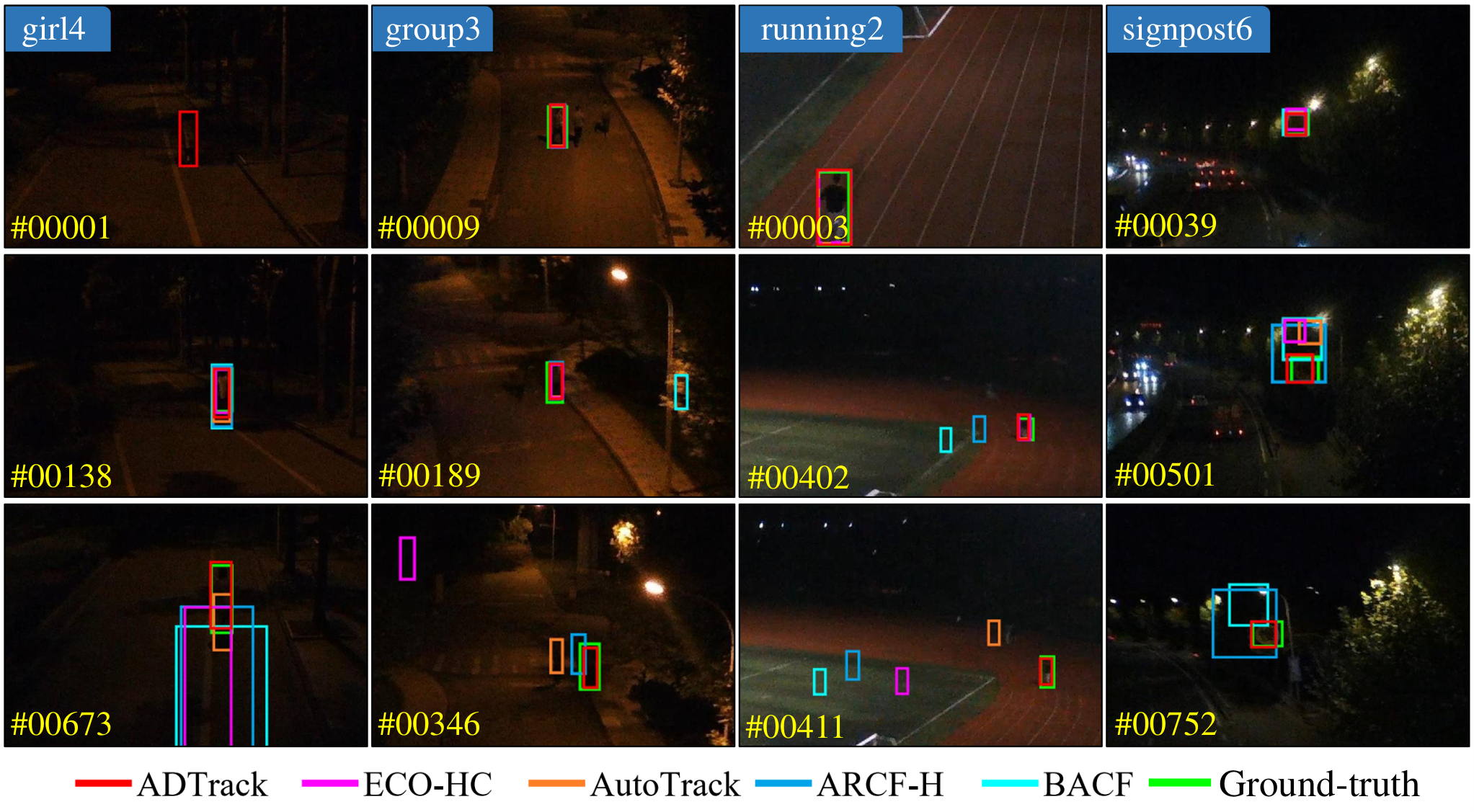
Benchmark UAVDark70 is newly made in this work, consisting of 70 manually annotated sequences. All the scenes were shot from a professional grade UAV at night. In Fig. 4( $a$ ), ADTrack outperforms all other arts and improves the baseline BACF [8] tracker by 10.2% under distance precision (DP) at center location error (CLE) = 20 pixels. In terms of area under curve (AUC), ADTrack ranks the first as well. Fig. 5 displays some typical dark tracking scenes and performance of the SOTA trackers in UAVDark70.

In order to maintain the objectivity, this work selected typical night scenes from the authoritative publicly available benchmark UAVDT [34] and Visdrone-2019SOT [35] (totally 37 sequences), and composed them into a new benchmark, i.e., UAVDark. In Fig. 4( $b$ ), ADTrack outperforms all others in both DP and AUC. Specifically, ADTrack improves the DP of baseline BACF by more than 4.5% in UAVDark.

TABLE I shows the top 11 hand-crafted CF-based trackers’ (both real-time and not real-time) venues and average results on 2 benchmarks, where ADTrack outperforms all other hand-crafted trackers. Besides, ADTrack achieves a speed of 34 FPS, meeting real-time requirement on UAV tracking.

Remark 5: The sequences in the newly made UAVDark70 are more common in real-world dark tracking, where the scenes are generally much darker, bringing more challenges to trackers.

TABLE I: Average results of the selected top 11 trackers using hand-crafted feature. Red, green, and blue respectively mean the first, second and third place. The FPS values in this table are all obtained on a single CPU.

Tracker	ADTrack	AutoTrack[4]	ARCF-HC[5]	ARCF-H[5]	STRCF[9]	MCCT-H[29]	BACF [8]	CSR-DCF [24]	Staple_CA [31]	ECO-HC [19]	Staple [30]
Venue	Ours	’20 CVPR	’19 ICCV	’19 ICCV	’18 CVPR	’18 CVPR	’17 ICCV	’17 CVPR	’17 CVPR	’17 CVPR	’16 CVPR
AUC	0.504	0.492	0.497	0.468	0.492	0.399	0.484	0.428	0.412	0.457	0.431
DP	0.749	0.728	0.722	0.705	0.706	0.600	0.699	0.650	0.622	0.666	0.656
FPS	34.84	49.05	24.71	38.58	22.84	47.16	41.52	8.42	48.99	57.52	85.16

IV-C Analysis by Attributes

TABLE II: Results comparison of the top 8 real-time hand-crafted CF-based trackers on UAVDark70 and UAVDark by UAV-specific attribute. Red, green, and blue respectively mean the first, second and third place. The results here are the average by all sequences involved.

	AUC					DP
	IV	OCC	LR	FM	VC	IV	OCC	LR	FM	VC
Staple [30]	0.436	0.396	0.356	0.433	0.421	0.656	0.561	0.633	0.613	0.632
ECO-HC [19]	0.443	0.437	0.363	0.457	0.437	0.580	0.558	0.586	0.620	0.633
Staple_CA [31]	0.415	0.410	0.359	0.425	0.396	0.563	0.511	0.622	0.592	0.591
BACF [8]	0.482	0.444	0.406	0.483	0.457	0.677	0.607	0.648	0.660	0.663
MCCT-H [29]	0.393	0.398	0.322	0.409	0.377	0.591	0.531	0.578	0.567	0.565
ARCF-H [5]	0.465	0.453	0.373	0.487	0.447	0.689	0.617	0.660	0.671	0.671
AutoTrack [4]	0.479	0.460	0.441	0.487	0.470	0.701	0.638	0.709	0.688	0.698
ADTrack (ours)	0.497	0.459	0.444	0.503	0.485	0.731	0.638	0.720	0.712	0.722

Following [21], this work considers the UAV special tracking challenges as low resolution (LR), fast motion (FM), illumination variation (IV), viewpoint change (VC), and occlusion (OCC). In terms of UAVDark70, the attributes are manually annotated according to the same criterion in [35]. TABLE II exhibits the average by sequences results of the top 8 real-time CF-based trackers in UAVDark and UAVDark70 according to TABLE I, where ADTrack ranks the first in most attributes.

IV-D Ablation Studies

This part exhibits the validity of different components in ADTrack on tracking. BACF_e denotes adding only the enhancing factor on the baseline tracker BACF [8]. ADTrack_e means ADTrack without dual filters (considered the Baseline). ADTrack_ew indicates adding merely weighted summation in detection stage on ADTrack_e. ADTrack means the full version of the proposed tracker (both weighted summation and constraint term). The results are displayed in TABLE III, where clearly, the proposed 2 components have boosted tracking performance by a large margin, improving more than 3% in both AUC and DP.

Remark 6: BACF_e is worse than original BACF, probably due to the noise introduced by image enhancing. While for ADTrack, the mask can block such negative effect.

TABLE III: AUC and DP comparison of different versions of ADTrack on UAVDark70. The tracker ADTrack_e, ADTrack_ew respectively denote ADTrack with different components.

Tracker	ADTrack	ADTrack_ew	ADTrack_e	BACF_e	BACF
AUC	0.502	0.492	0.487	0.448	0.451
$\Delta$ (%)	+11.3	+9.0	+7.9	-0.7	0
DP	0.712	0.694	0.689	0.618	0.630
$\Delta$ (%)	+13.0	+10.2	+9.4	-1.9	0

IV-E Against the Deep Trackers

This section focuses on comparison between proposed ADTrack and deep trackers which utilize off-line trained deep network for feature extraction or template matching. This work invites totally 10 SOTA deep trackers, i.e., SiameseFC [6], ASRCF [7], ECO [19], UDT+ [36], TADT [37], UDT [36], HCFT [38], IBCCF [39], and DSiam [40], to test their performance in UAVDark. From TABLE IV, ADTrack clearly outperforms most deep trackers in terms of DP and AUC.

Remark 7: Using merely single CPU, ADTrack still achieves a real-time speed at more than 30 FPS, while many deep trackers are far from real-time even on GPU, demonstrating the excellence of ADTrack for real-time UAV tracking.

TABLE V selects the top 5 trackers in TABLE IV to evaluate their performance under the newly constructed UAVDark70.

Remark 8: The results illustrate that the SOTA deep trackers fail to maintain their robustness in real-world common dark scenes, since the CNNs they utilize are trained by daytime images, ending up in their huge inferiority compared with online-learned ADTrack in the dark.

TABLE IV: AUC, DP, and tracking speed (FPS) comparison of the deep trackers and ADTrack on UAVDark. * denotes GPU speed, which is not commonly used in UAV platform. Red, green, and blue respectively mean the first, second and third place.

Tracker	Venue	DP	AUC	FPS	GPU
HCFT [38]	’15 ICCV	0.721	0.451	18.26*	✓
SiameseFC [6]	’16 ECCV	0.713	0.467	37.17*	✓
IBCCF [39]	’17 ICCV	0.731	0.474	2.77*	✓
DSiam [40]	’17 ICCV	0.653	0.419	15.62*	✓
ECO [19]	’17 CVPR	0.790	0.498	16.12*	✓
UDT [36]	’19 CVPR	0.754	0.484	56.68*	✓
TADT [37]	’19 CVPR	0.780	0.498	29.06*	✓
UDT+ [36]	’19 CVPR	0.728	0.459	53.96*	✓
ASRCF [7]	’19 CVPR	0.775	0.500	21.39*	✓
ADTrack	Ours	0.786	0.505	37.71	✗

TABLE V: AUC and DP comparison of top 5 trackers in TABLE. IV on UAVDark70. Red, green, and blue respectively mean the first, second and third place.

Tracker	ADTrack	ECO [19]	TADT [37]	ASRCF [7]	UDT [36]
AUC	0.502	0.446	0.403	0.493	0.298
DP	0.712	0.612	0.532	0.678	0.390

V Conclusion

This work puts forward a novel real-time tracker with anti-dark function, i.e., ADTrack. ADTrack first implements image enhancement and target-aware mask generation based on an image enhancer. With the mask, ADTrack innovatively proposes dual filters, i.e., the target-focused filter and the context filter, regression model. Thus, the dual filters restrict each other in training and compensate each other in detection, achieving robust real-time dark tracking onboard UAV. In addition, the first dark tracking benchmark, UAVDark70, is also constructed in this work for visual tracking community. The proposed anti-dark tracker and dark tracking benchmark will make an outstanding contribution to the research of UAV tracking in dark conditions in the future.

Acknowledgment

This work is supported by the National Natural Science Foundation of China (No. 61806148) and Natural Science Foundation of Shanghai (No. 20ZR1460100).

References

[1] T. Baca, D. Hert, G. Loianno, M. Saska, and V. Kumar, “Model Predictive Trajectory Tracking and Collision Avoidance for Reliable Outdoor Deployment of Unmanned Aerial Vehicles,” in 2018 IEEE/RSJ International Conference on Intelligent Robots and Systems (IROS), 2018, pp. 6753–6760.
[2] D. R. McArthur, Z. An, and D. J. Cappelleri, “Pose-Estimate-Based Target Tracking for Human-Guided Remote Sensor Mounting with a UAV,” in Proceedings of IEEE International Conference on Robotics and Automation (ICRA), 2020, pp. 10 636–10 642.
[3] J. Bian, X. Hui, X. Zhao, and M. Tan, “A Novel Monocular-Based Navigation Approach for UAV Autonomous Transmission-Line Inspection,” in Proceedings of IEEE/RSJ International Conference on Intelligent Robots and Systems (IROS), 2018, pp. 1–7.
[4] Y. Li, C. Fu, F. Ding, Z. Huang, and G. Lu, “AutoTrack: Towards High-Performance Visual Tracking for UAV with Automatic Spatio-Temporal Regularization,” in Proceedings of IEEE Conference on Computer Vision and Pattern Recognition (CVPR), 2020, pp. 11 923–11 932.
[5] Z. Huang, C. Fu, Y. Li, F. Lin, and P. Lu, “Learning Aberrance Repressed Correlation Filters for Real-Time UAV Tracking,” in Proceedings of the IEEE International Conference on Computer Vision (ICCV), 2019, pp. 2891–2900.
[6] L. Bertinetto, J. Valmadre, J. F. Henriques, A. Vedaldi, and P. H. S. Torr, “Fully-Convolutional Siamese Networks for Object Tracking,” in Proceedings of European Conference on Computer Vision (ECCV), 2016, pp. 850–865.
[7] K. Dai, D. Wang, H. Lu, C. Sun, and J. Li, “Visual Tracking via Adaptive Spatially-Regularized Correlation Filters,” in Proceedings of IEEE Conference on Computer Vision and Pattern Recognition (CVPR), 2019, pp. 4665–4674.
[8] H. K. Galoogahi, A. Fagg, and S. Lucey, “Learning Background-Aware Correlation Filters for Visual Tracking,” in Proceedings of IEEE International Conference on Computer Vision (ICCV), 2017, pp. 1144–1152.
[9] F. Li, C. Tian, W. Zuo, L. Zhang, and M. Yang, “Learning Spatial-Temporal Regularized Correlation Filters for Visual Tracking,” in Proceedings of IEEE Conference on Computer Vision and Pattern Recognition (CVPR), 2018, pp. 4904–4913.
[10] Y. Zhang, J. Zhang, and X. Guo, “Kindling the Darkness: A Practical Low-Light Image Enhancer,” in Proceedings of the ACM International Conference on Multimedia (ACM), 2019, pp. 1632–1640.
[11] S. Park, S. Yu, M. Kim, K. Park, and J. Paik, “Dual Autoencoder Network for Retinex-Based Low-Light Image Enhancement,” IEEE Access, vol. 6, pp. 22 084–22 093, 2018.
[12] M. Li, J. Liu, W. Yang, X. Sun, and Z. Guo, “Structure-Revealing Low-Light Image Enhancement Via Robust Retinex Model,” IEEE Transactions on Image Processing, vol. 27, no. 6, pp. 2828–2841, 2018.
[13] E. H. Land, “The Retinex Theory of Color Vision,” Scientific American, vol. 237, no. 6, pp. 108–129, 1977.
[14] H. Ahn, B. Keum, D. Kim, and H. S. Lee, “Adaptive Local Tone Mapping Based on Retinex for High Dynamic Range Images,” in Proceedings of IEEE International Conference on Consumer Electronics (ICCE), 2013, pp. 153–156.
[15] D. S. Bolme, J. R. Beveridge, B. A. Draper, and Y. M. Lui, “Visual Object Tracking Using Adaptive Correlation Filters,” in Proceedings of IEEE Conference on Computer Vision and Pattern Recognition (CVPR), 2010, pp. 2544–2550.
[16] J. F. Henriques, R. Caseiro, P. Martins, and J. Batista, “High-Speed Tracking with Kernelized Correlation Filters,” IEEE Transactions on Pattern Analysis and Machine Intelligence, vol. 37, no. 3, pp. 583–596, 2015.
[17] M. Danelljan, G. Häger, F. S. Khan, and M. Felsberg, “Learning Spatially Regularized Correlation Filters for Visual Tracking,” in Proceedings of IEEE International Conference on Computer Vision (ICCV), 2015, pp. 4310–4318.
[18] M. Danelljan, G. Häger, F. S. Khan, and M. Felsberg, “Discriminative Scale Space Tracking,” IEEE Transactions on Pattern Analysis and Machine Intelligence, vol. 39, no. 8, pp. 1561–1575, 2017.
[19] M. Danelljan, G. Bhat, F. Shahbaz Khan, and M. Felsberg, “ECO: Efficient Convolution Operators for Tracking,” in Proceedings of IEEE Conference on Computer Vision and Pattern Recognition (CVPR), 2017, pp. 6638–6646.
[20] C. Fu, J. Xu, F. Lin, F. Guo, T. Liu, and Z. Zhang, “Object Saliency-Aware Dual Regularized Correlation Filter for Real-Time Aerial Tracking,” IEEE Transactions on Geoscience and Remote Sensing, pp. 1–12, 2020.
[21] C. Fu, B. Li, F. Ding, F. Lin, and G. Lu, “Correlation Filter for UAV-Based Aerial Tracking: A Review and Experimental Evaluation,” arXiv preprint arXiv:2010.06255, pp. 1–28, 2020.
[22] C. Fu, J. Ye et al., “Disruptor-Aware Interval-Based Response Inconsistency for Correlation Filters in Real-Time Aerial Tracking,” IEEE Transactions on Geoscience and Remote Sensing, pp. 1–13, 2020.
[23] F. Ding, C. Fu, Y. Li, J. Jin, and C. Feng, “Automatic Failure Recovery and Re-Initialization for Online UAV Tracking with Joint Scale and Aspect Ratio Optimization,” in Proceedings of IEEE/RSJ International Conference on Intelligent Robots and Systems (IROS), 2020, pp. 1–8.
[24] A. Lukezic, T. Vojir, L. Cehovin Zajc, J. Matas, and M. Kristan, “Discriminative Correlation Filter with Channel and Spatial Reliability,” in Proceedings of IEEE Conference on Computer Vision and Pattern Recognition (CVPR), 2017, pp. 6309–6318.
[25] E. Reinhard, M. Stark, P. Shirley, and J. Ferwerda, “Photographic Tone Reproduction for Digital Images,” in Proceedings of the annual conference on Computer graphics and interactive techniques (ACM), 2002, pp. 267–276.
[26] S. Boyd, N. Parikh, E. Chu, B. Peleato, and J. Eckstein, “Distributed Optimization and Statistical Learning via the Alternating Direction Method of Multipliers,” Foundations and Trends in Machine Learning, vol. 3, pp. 1–122, 2010.
[27] J. Sherman and W. J. Morrison, “Adjustment of An Inverse Matrix Corresponding to A Change in One Element of A Given Matrix,” The Annals of Mathematical Statistics, vol. 21, no. 1, pp. 124–127, 1950.
[28] C. Wang, L. Zhang, L. Xie, and J. Yuan, “Kernel Cross-Correlator,” in Proceedings of AAAI Conference on Artificial Intelligence (AAAI), 2018, pp. 1–8.
[29] N. Wang, W. Zhou, Q. Tian, R. Hong, M. Wang, and H. Li, “Multi-cue Correlation Filters for Robust Visual Tracking,” in Proceedings of IEEE Conference on Computer Vision and Pattern Recognition (CVPR), 2018, pp. 4844–4853.
[30] L. Bertinetto, J. Valmadre, S. Golodetz, O. Miksik, and P. H. Torr, “Staple: Complementary Learners for Real-time Tracking,” in Proceedings of IEEE Conference on Computer Vision and Pattern Recognition (CVPR), 2016, pp. 1401–1409.
[31] M. Mueller, N. Smith, and B. Ghanem, “Context-Aware Correlation Filter Tracking,” in Proceedings of IEEE Conference on Computer Vision and Pattern Recognition (CVPR), 2017, pp. 1396–1404.
[32] P. F. Felzenszwalb, R. B. Girshick, D. McAllester, and D. Ramanan, “Object Detection with Discriminatively Trained Part-Based Models,” IEEE Transactions on Pattern Analysis and Machine Intelligence, vol. 32, no. 9, pp. 1627–1645, 2010.
[33] J. van de Weijer and C. Schmid, “Coloring Local Feature Extraction,” in Proceedings of European Conference on Computer Vision (ECCV), 2006, pp. 334–348.
[34] D. Du, Y. Qi, H. Yu, Y. Yang, K. Duan, G. Li, W. Zhang, Q. Huang, and Q. Tian, “The Unmanned Aerial Vehicle Benchmark: Object Detection and Tracking,” in Proceedings of the European Conference on Computer Vision (ECCV), 2018, pp. 370–386.
[35] D. Du, P. Zhu et al., “VisDrone-SOT2019: The Vision Meets Drone Single Object Tracking Challenge Results,” in Proceedings of International Conference on Computer Vision Workshops (ICCVW), 2019, pp. 1–14.
[36] N. Wang, Y. Song, C. Ma, W. Zhou, W. Liu, and H. Li, “Unsupervised Deep Tracking,” in Proceedings of IEEE Conference on Computer Vision and Pattern Recognition (CVPR), 2019, pp. 1308–1317.
[37] X. Li, C. Ma, B. Wu, Z. He, and M.-H. Yang, “Target-Aware Deep Tracking,” in Proceedings of IEEE Conference on Computer Vision and Pattern Recognition (CVPR), 2019, pp. 1369–1378.
[38] C. Ma, J. Huang, X. Yang, and M. Yang, “Hierarchical Convolutional Features for Visual Tracking,” in Proceedings of IEEE International Conference on Computer Vision (ICCV), 2015, pp. 3074–3082.
[39] F. Li, Y. Yao, P. Li, D. Zhang, W. Zuo, and M.-H. Yang, “Integrating Boundary and Center Correlation Filters for Visual Tracking with Aspect Ratio Variation,” in Proceedings of IEEE International Conference on Computer Vision Workshops (ICCVW), 2017, pp. 2001–2009.
[40] Q. Guo, W. Feng, C. Zhou, R. Huang, L. Wan, and S. Wang, “Learning Dynamic Siamese Network for Visual Object Tracking,” in Proceedings of IEEE International Conference on Computer Vision (ICCV), 2017, pp. 1781–1789.