Evaluating Local Explanations using White-box ModelsDOI: 10.1145/1122445.1122456Conference: Woodstock ’18: ACM Symposium on Neural Gaze Detection; June 03–05, 2018; Woodstock, NYWoodstock ’18: ACM Symposium on Neural Gaze Detection, June 03–05, 2018, Woodstock, NYPrice: 15.00ISBN: 978-1-4503-XXXX-X/18/06CCS: Computing methodologies Modeling methodologies
Abstract.
Evaluating explanation techniques using human subjects is costly, time-consuming and can lead to subjectivity in the assessments. To evaluate the accuracy of local explanations, we require access to the true feature importance scores for a given instance. However, the prediction function of a model usually does not decompose into linear additive terms that indicate how much a feature contributes to the output. In this work, we suggest to instead focus on the log odds ratio (LOR) of the prediction function, which naturally decomposes into additive terms for logistic regression and naive Bayes. We demonstrate how we can benchmark different explanation techniques in terms of their similarity to the LOR scores based on our proposed approach. In the experiments, we compare prominent local explanation techniques and find that the performance of the techniques can depend on the underlying model, the dataset, which data point is explained, the normalization of the data and the similarity metric.
Keywords:
explainability, interpretability, machine learning1. Introduction
As machine learning models have become more complex, the need for techniques that explain the decision making process of the these black-boxes has grown. To make the decision making process more accessible to humans, explanation techniques can be used to estimate the importance of input features to a model’s output. Explanation techniques fall into two main categories: global or local explanations. Global explanations are a set of feature importance scores that are important for in the prediction of all instances in a dataset (Craven and Shavlik 1995). Local explanations are the set of feature importance scores that are important in the prediction of a single instance from a dataset (Ribeiro et al. 2016b). One prominent class of local explanation techniques are local additive explanations that fit a linear - or additive - model to the predictions of the underlying model for a given instance (Lundberg and Lee 2017).

In order to evaluate the accuracy of explanations, two categories of evaluation methods have been proposed: human-grounded and functionally-grounded (Doshi-Velez and Kim 2017). Human-grounded evaluation methods use the judgment of human subjects to evaluate the accuracy of explanations. The subjectivity of human judgment, time, and costs make human-grounded evaluations often infeasible. Functionally-grounded methods use different proxy measures to evaluate explanation techniques systematically. Compared to human-grounded methods, functionally-grounded methods are fast and less costly. Functionally grounded evaluation methods are specifically useful in the early development of explanation techniques.
As we discuss in Section 2, existing functionally-grounded methods cannot directly assess explanation accuracy. To assess accuracy directly, we need to have access to the ground truth (Bishop 2006). In the context of explanations, this ground truth consists of the true feature importance scores for a given instance and prediction function. If we had access to a prediction function that decomposes into a linear weighted sum of the true importance scores, we would expect an accurate local additive explanation technique applied to this function to output scores that are not far from these true importance scores. The latter could thus be used to evaluate the accuracy of explanations. Since the prediction function of even simple classification models is not linear, we cannot directly assess accuracy based on the prediction function. In this work we propose to explain not the prediction function, but the log odds ratio (LOR) thereof. In particular, we focus on explaining two white-box models, logistic regression and naive Bayes, for which the log odds ratio decomposes into a linear sum of terms. These terms indicate how much a feature contributes to the prediction of one class versus another. We can thus interpret these additive log odds ratio (aLOR) terms as the true feature importance of the log odds ratio11 1 The aLOR terms are also referred to as true importance scores or aLOR scores throughout our study.. Given the true importance scores, we are now able to determine the accuracy of local additive explanation techniques. In our proposed method, we start by extracting the aLOR terms and local additive explanations based on the log odds ratio as shown in Step 1 and 2 in Figure 1. These can then be compared in terms of similarity as shown in Step 3 in Figure 1. We suggest to use our method as an initial verification of a new explanation technique which can be complemented with human- or other functionally-grounded evaluation techniques at later stages.
We perform an extensive comparison of three local model-agnostic explanation techniques across 20 datasets; Local Interpretable Model-agnostic Explanations (LIME) (Ribeiro et al. 2016a), SHapley Additive exPlanations (SHAP) (Lundberg and Lee 2017) and Local Permutation Importance (LPI) (Casalicchio et al. 2018). It is important to state that while LPI explanations are not additive, we are still interested to include LPI as a prominent local explanation technique. Our key findings from this investigation are: 1) The performance of LIME and SHAP varies to a large extent across datasets, data points and underlying models. In some cases, the Spearman’s rank correlation between LIME and SHAP explanations and aLOR terms is small or even negative. 2) LPI provides more accurate explanations relative to LIME and SHAP when the chosen similarity metric is Spearman’s Rank Correlation. 3) LIME explanations provide more accurate explanations relative to SHAP and LPI when the chosen similarity metric is Euclidean or Cosine Similarity 4) The employed preprocessing technique has a large effect on the explanation accuracy, especially in the case of Logistic Regression. 5) The notions of robustness and accuracy of explanation techniques are complementary and orthogonal to one another
In the next section, we discuss related work on local model-agnostic explanation techniques and functionally-grounded evaluation. We then formally introduce the proposed evaluation method in Section 3. In Section 4, we empirically study the accuracy of explanation techniques in 20 datasets based on our proposed approach. We discuss the proposed method further in Section 5, and finally, we summarize the main conclusions and point out directions for future research in Section 6.
2. Local model-agnostic explanations and functionally-grounded evaluation
Local additive model-agnostic explanation techniques decompose the predicted probability of a black-box model into an additive sum of feature importance scores of a single instance (Lundberg and Lee 2017). Throughout this paper, the notion of local additive explanations and local additive model-agnostic explanations are used interchangeably. LIME and SHAP are examples of widely used techniques to obtain additive explanations. The explanations of LIME and SHAP consist of the weights of a local linear model that is trained to imitate the decision boundary of the black-box model for a given instance. In contrast, LPI defines the importance of a feature to be the average decrease in the prediction score when this feature value is randomly replaced by a different value (Casalicchio et al. 2018). It is important to acknowledge that the feature importance scores of non-additive explanation techniques such as LPI have a different interpretation compared to additive explanation techniques.
To evaluate the quality of explanations, functionally-grounded methods have been proposed. We have classified these method into two main categories: ablation and robustness evaluation techniques. Ablation techniques measure the sensitivity of the model’s predicted value after the removal of features with high importance scores (Hsieh et al. 2021). The rationale behind this evaluation method is that the more substantial the change of the model’s predicted value following the removal of important features, the more accurate are the explanations. Different ablation techniques are proposed in the literature of explainability which are different variations of the Occlusion Sensitivity method proposed in (Zeiler and Fergus 2014). Ablation techniques therefore measure the accuracy of explanations indirectly, meaning without access to the ground truth. One example of this technique is presented in (Hooker et al. 2019). The authors propose RemOve And Retrain (ROAR) to evaluate different explanation techniques based on saliency maps. The black-box model is retrained on an auxiliary dataset that is striped of pixels deemed important by the explanations. The accuracy of the explanations is calculated as the difference between the predicted class probabilities of the original and the auxiliary instance. Methods such as ROAR are computationally expensive as the underlying model needs to be retrained on a large auxiliary data set. Another limitation of this evaluation method is that the new auxiliary data and retrained black-box model deviate from the original data and model and can exhibit new structures or properties.
Robustness of explanations on the other hand measures the difference in explanations of a single instance after adding noise or redundancy to the features of the explained instance (Alvarez-Melis and Jaakkola 2018; Camburu et al. 2019). The main rationale behind this category of evaluation techniques is that a robust explanation technique should provide explanations that are resilient with respect to the added noise and assign relatively low importance scores to redundant features. (Alvarez-Melis and Jaakkola 2018) empirically show that some explanation techniques including LIME are not robust to Lipschitz noise. In (Camburu et al. 2019), the robustness of LIME, SHAP and Learn To eXplain (L2X) (Chen et al. 2018) is studied following the introduction of irrelevant features to the explained instance in a sentiment analysis task. According to the results, L2X explanations outperform other explanation techniques across different measures of robustness that are proposed in the study. One limitation of this category of evaluation techniques is that changing the feature values of the input instance can turn it into an out-of-distribution data point. This can lead to highly uncertain predictions by the black-box model which makes it impossible to distinguish between a failing black-box and a failing explanation (Lakkaraju et al. 2020; Rahnama and Boström 2019). In section 4.3, we perform experiments that measure the robustness of the explanation techniques in this study.
Both classes of techniques suffer from the fact that there is no objective way to directly derive the accuracy of an explanation solely based on the change of the black-box’s output. Changing a feature value deemed important by an explanation does not necessarily lead to a change in the model’s output. Similarly, if changing the feature moves the data point off the training data manifold, the output of the black-box might change dramatically (Lipton et al. 2018).
In contrast to ablation and robustness methods, we propose an evaluation method that extracts the true importance scores from the LOR and compares them directly to local explanations obtained from other explanation techniques.
3. Methodology
To evaluate the accuracy of a local model-agnostic explanation technique, we propose to extract the true importance scores of the LOR of two white-box models, logistic regression and naive Bayes. These scores are compared to local additive explanations obtained from the LOR of these white-box models (see Section 3.3). We use Euclidean and Cosine Similarity along with Spearman’s Rank correlation (see Section 3.4) to assess the accuracy of the explanations with respect to the true importance scores. If the explanations correlate highly with the true importance scores, we can conclude that the explanation is accurate. Figure 2 shows a visualization of the true importance scores of a single instance as well as LIME, SHAP and LPI explanations.
3.1. Local additive explanations
Since LIME and SHAP are examples of local additive explanations, we present a formalization of local additive explanations based on the notation used in (Lundberg and Lee 2017). Let be a matrix of data points with corresponding features and be a vector of binary labels. Suppose is an instance of and let denote the feature of . Assume that we want to explain the prediction of model for a given instance . The local additive explanation then has the form:
| (1) |
where is a simplified version of and the prediction should be close to the prediction of the original function , i.e., . We denote the explanation by .
In practice, a subset of is selected including the top- ranked elements based on the absolute value of importance scores, where (Ribeiro et al. 2016a). It is important to note that we extract the local model-agnostic explanations based on the log odds ratio of a single instance with respect to a specific class instead of the class probability scores . This is necessary as the extracted LOR scores are based on the log odds ratio.
3.2. Local Permutation Importance
The core idea behind LPI (Casalicchio et al. 2018) is that the importance of a certain feature can be estimated by the average change of a black-box’s prediction given that the value of this feature is replaced by another value. To change the feature value, LPI randomly permutates feature values of a single dimension across all data points.
We calculate LPI as follows. Let be a random permutation of the index sequence , and let denote the position of index in . The importance of feature at is then defined as:
| (2) |
where is defined as follows:
| (3) |
where and . In simpler terms, is equal to except that the value of the th feature is replaced by . It is noteworthy that we make use of the model’s log odds ratio of class instead of the predicted values .

3.3. True Importance Scores
The weights of logistic regression and naive Bayes models can be used as global explanations to understand which features are important in their learning and prediction process (Freitas 2014). In our study, we propose to obtain the feature importance scores for a single data point from these models. Since the prediction functions of logistic regression and naive Bayes do not naturally decompose into additive terms, we turn the task of explaining the models’ prediction function into the task of explaining the log odds ratio functions. We demonstrate that the log odds ratio can indeed decompose into additive parts for logistic regression and naive Bayes. As a result, each of the additive parts corresponds to a single feature and expresses how much the feature contributes to predicted log odds ratio of one class versus another. We call these terms additive Log Odds Ratio (aLOR) scores. Please note that while the notation in this section is based on a binary setting, however our proposed approach is extended to a multi-class settings using a one-vs-rest (OvR) method.
3.3.1. Logistic regression
Given weights and an instance , the prediction function of a logistic regression model is defined as
| (4) |
where we define . We can derive an additive decomposition of the prediction function by using the log odds ratio for with respect to class :
| (5) |
where is the complement of class and is the local importance score for feature . The extracted aLOR scores are denoted by .
3.3.2. Naive Bayes
Given input and a mean and variance vector, and , the prediction function of naive Bayes is defined as
| (6) |
where the likelihood is given by
| (7) |
Similar to the case of logistic regression, the prediction function does not naturally decompose into additive parts. However, the log odds ratio for an instance with respect to class has an intrinsic natural additive decomposition,
| (8) |
where . Based on this, the importance score for feature is .
In our comparison, we compare each term with from Equation 1 since our proposed decomposition terms include two terms, namely the weight times the explained input. In each decomposed terms from Equation 1, is a simplified binary vector of one. This is due to the fact that local additive explanation do not provide an explanation for features with zero values (Lundberg and Lee 2017; Ribeiro et al. 2016a).
3.3.3. Example
To make our idea more tangible, we train a logistic regression model with L2 regularization on a 2-dimensional discrete logical AND function that returns one if both inputs are one and zero otherwise. The parameters of the logistic regression model are and with intercept value . These parameters show that the model correctly learned that both features are equally important on a global level. For with and the model predicts . Based on this, we can derive the log odds ratio for as
We can see that, whereas the first and second feature are equally important globally, the only feature that contributes to the log odds prediction is the first feature. The resulting aLOR scores consist of and the feature importance scores of the log odds ratio of with respect to class . A similar example for naive Bayes can be found in the Appendix.
3.4. Evaluating explanation accuracy
As discussed before, we suggest to use the aLOR scores as true importance scores when comparing explanation techniques. In order to measure the similarity between the true importance scores and different explanations, we use Euclidean and Cosine similarity along with Spearman’s Rank correlation. We suggest to use the Spearman’s Rank correlation as the primary measure of similarity (see Sections 3.4.1 and 3.4.2). We explain how we can use the aLOR scores to evaluate the relative performance of explanation techniques in a systematic manner in Section 3.4.3.
3.4.1. Similarity between explanations
We measure accuracy in terms of how similar an explanation is to the true importance scores. Similarity between explanations can be measured in different ways. Several studies have used measures such as Cosine or Euclidean distance (Montavon et al. 2018; Yang and Kim 2019) to measure the similarity of explanations. Similar to arguments in (Ghorbani et al. 2019), we argue that the Spearman’s Rank correlation is the most suitable measure for comparing explanations. This is because in numerous applications, explanations are presented as a small subset of ranked features based on their absolute importance scores (Ribeiro et al. 2016a). Based on this, we may not need to pay attention to small changes in the importance scores that do not change the ranking of the features. In addition, a mistake in assigning low importance scores to a highly important features need to have a larger effect than of a assigning a wrong importance scores to modestly important features. The Spearman’s Rank correlation coefficient is optimal in this setting as it is not affected by small, rank-preserving differences between explanations or differences in scale whereas such differences might affect cosine similarity or Euclidean distance drastically. Cosine and Euclidean distances are useful in applications where the explanations are not ranked based on importance scores but represented as vectors that include all features.
Additionally, the interpretation of explanations might differ across different types of explanation techniques. Rank correlation makes it possible to compare feature importance scores between additive and non-additive explanations techniques which otherwise cannot be compared directly. Lastly, correlation has a natural interpretation of how similar two vectors are and is confined to the interval between -1 and 1. In contrast to e.g. Cosine and Euclidean similarity, correlation comes with interpretable measures of direction and strength. One drawback of using a rank-based measure is that it might be sensitive in case a dataset has many unimportant feature dimensions. In this case, the performance across all explanation techniques will be low as the ranking of unimportant features will vary randomly. As we show in the next section, at least one of the techniques usually has an average correlation of more than 0.4 for a given dataset, indicating that unimportant features do not impact explanation accuracy for the datasets chosen in this study.
3.4.2. Example
To understand the difference between the Euclidean and Cosine similarity along with Spearman’s rank correlation, imagine we want to compare two different explanations and to the aLOR score .
As can be seen, the ranking of correlates perfectly with , while the ranking of is negatively correlated with . When using this rank-based metric, we can thus conclude that explanation is more accurate than .
3.4.3. Evaluation procedure
On a high level, to evaluate an explanation technique using the log odds ratio of white-box model , we extract the aLOR scores and the local model-agnostic explanation for a single instance . We then compute the similarity between and using Spearman’s rank correlation . We measure the Spearman’s rank correlation based on the absolute importance scores since that is how explanations are presented (Ribeiro et al. 2016a). This procedure is detailed in Algorithm 1.
In general, we are interested in comparing different explanation techniques based on their similarity to the aLOR scores extracted from a white-box model across several datasets. Let be the th dataset of datasets. Suppose we obtain by applying Algorithm 1 to test instances of the th dataset for each explanation technique . The average value of can be seen as a measure of how accurate the explanation technique is with respect to the aLOR scores. Needless to say, the higher the average values of are, the more accurate are the explanations when explaining model .
Input : instance
Functions : white-box model, : explanation method, : function to extract aLOR scores
: Spearman’s rank correlation
Output : correlation value
3.5. Explanation Robustness
In this section, we present formal definitions of the robustness measures that are used in our experiments.
Local Lipschitz was proposed by (Alvarez-Melis and Jaakkola 2018) to measure the maximum change in the predicted probability score of a black-box model in a neighbourhood around the explained instance. Let denote a sample of inputs and for every let its neighbourhood be
| (9) |
can also be created by adding Gaussian noise to the input sample and there is no need to set an in this case (see (Alvarez-Melis and Jaakkola 2018) for details). Local Lipschitz is then defined as
| (10) |
where is the black-box model that outputs a probability score for a designated class. While there is no ideal value, lower Local Lipschitz values indicate that an explanation technique is more robust.
We consider two additional measures of robustness, namely and 22 2 These measures are refereed to as and for brevity in Table 3 that are originally proposed by (Fong and Vedaldi 2017; Samek et al. 2016). Our notation is similar to that in (Hsieh et al. 2021). Let be the set of important features selected by an explanation technique and let . measures the change in the predicted probability scores of a black-box after the replacement of feature values in with a baseline value. Similarly, reflects the change in the predicted probability score of a black-box following the replacement of feature values in with a baseline. The baseline value can be binary or the average value of the corresponding feature in the training or validation set. Similar to the case of Local Lipschitz, there are no ideal optimal values for these robustness measures. It is then defined that robust explanations have relatively large values and low .
| Model | Logistic Regression | Naïve Bayes | ||||
|---|---|---|---|---|---|---|
| Dataset | LIME | SHAP | LPI | LIME | SHAP | LPI |
| Adult | 0.27 | 0.221 | 0.203 | 0.724 | 0.401 | 0.752 |
| Attrition | 0.502 | 0.194 | 0.423 | 0.261 | 0.297 | 0.297 |
| Audit | 0.515 | 0.511 | 0.703 | 0.194 | 0.382 | 0.55 |
| Banking | 0.226 | 0.477 | 0.338 | 0.486 | 0.088 | 0.848 |
| Banknote | 0.81 | 0.898 | 0.778 | 0.908 | 0.778 | 0.904 |
| Breast Cancer | 0.811 | 0.833 | 0.803 | 0.688 | 0.687 | 0.455 |
| Churn | 0.331 | 0.133 | 0.409 | 0.692 | 0.536 | 0.651 |
| Donors | 0.048 | 0.346 | 0.51 | 0.131 | 0.304 | 0.556 |
| HR | 0.092 | 0.264 | 0.315 | 0.774 | 0.275 | 0.675 |
| Haberman | 0.74 | 0.377 | 0.708 | 0.786 | 0.026 | 0.877 |
| Hattrick | 0.403 | 0.657 | 0.637 | 0.586 | 0.564 | 0.446 |
| Heart Disease | 0.322 | 0.134 | 0.33 | 0.785 | 0.424 | 0.623 |
| Insurance | 0.595 | -0.301 | 0.604 | 0.616 | 0.199 | 0.644 |
| Iris | 0.728 | 0.792 | 0.848 | 0.848 | 0.892 | 0.78 |
| Loan | 0.398 | 0.33 | 0.453 | 0.311 | 0.463 | 0.463 |
| Pima Indians | 0.775 | 0.856 | 0.593 | 0.743 | 0.469 | 0.606 |
| Seismic | 0.501 | 0.511 | 0.497 | 0.773 | 0.198 | 0.716 |
| Spambase | 0.606 | 0.244 | 0.552 | -0.259 | 0.182 | 0.463 |
| Thera | 0.488 | 0.208 | 0.557 | 0.306 | 0.48 | 0.48 |
| Titanic | 0.779 | 0.245 | 0.74 | 0.695 | 0.366 | 0.794 |
| Average | 0.497 | 0.396 | 0.55 | 0.552 | 0.401 | 0.629 |
| Standard Deviation | 0.23 | 0.293 | 0.176 | 0.293 | 0.216 | 0.162 |
4. Empirical Investigation
We start out by describing the experimental setup, which is followed by results from comparing the selected explanations techniques against true importance scores. Finally, we investigate the effect of the choice of preprocessing technique, used prior to model generation.
4.1. Experimental setup
In this section, we provide the results of our empirical investigation where we compare explanations of LIME, SHAP, and LPI when explaining logistic regression and naive Bayes models in terms of their accuracy33 3 The code for experiments is available at: https://anonymous.4open.science/r/Evaluation-Local-Explanations-Whitebox-Models-BFC5/.
We evaluate the proposed procedure on 20 different tabular datasets, all concerning classification tasks (binary and multi-class). Unless otherwise stated, the numerical features are standardized and categorical features are encoded as one-hot vectors. For datasets for which no separate test set has been provided at the source, a random hold-out set of 25% was used. In order to tune the hyper-parameters of the logistic regression models we use grid-search44 4 Hyper parameters were chosen after 10 trials with the hyper-parameter space consisting of L1 and L2 regularization with the regularization parameter selected from a uniform distribution of values between 0 to 4. . The Appendix includes the test accuracy of the logistic regression and naive Bayes models along with references to the datasets used in the experiments, which are all publicly available.
For LIME and SHAP, we used the official Python packages TabularLIME (Ribeiro et al. 2016b) and KernelShap (Lundberg and Lee 2017). We would like to emphasize that KernelShap explainer is model-agnostic and it outputs approximated SHAP values. This is contrast to model-based explainers such as LinearSHAP where the SHAP values are analytically deducible from closed-form equations (see (Lundberg and Lee 2017) for details). In our study, we are comparing model-agnostic explanations where the explainers have no assumptions on the class of machine learning models they are explaining. The number of samples generated for LIME and SHAP is 5000 as suggested in (Lundberg and Lee 2017; Ribeiro et al. 2016b). In the case of LPI, it is the size of the training set as suggested in (Casalicchio et al. 2018). This means the sample size of LPI is half the size of LIME and SHAP on average. As stated earlier, the feature importance scores are extracted from the log odds ratios of instances with respect to a specific class. Therefore we need to obtain the local explanations based on the log odds ratio of a given class. In the case of binary classification, we explain the class designated as one in the dataset to be in line with equations in Section 3.3.1 and 3.3.2. In the case of multi-class classification, the predicted class by the underlying model is explained. The only modification we have made is to pass the log odds ratio function as a replacement of the prediction function when obtaining explanations. This is possible as in both packages one can pass in any desired prediction function when obtaining explanations. In the case of LPI, we have replicated the algorithm proposed in (Casalicchio et al. 2018) such that the importance scores are calculated based on the log odds ratio scores instead of the prediction function (see Section 3.2).
4.2. General performance
The average rank correlations for all datasets and explanation techniques are presented in Table 1. The first three columns list the results for the logistic regression white-box models and the last three columns list the equivalent for the naive Bayes white-box models. We also summarize the average rank correlation values across all datasets as well as the standard deviation in the last two rows.
Let us first focus on the explanations of the two local additive techniques, LIME and SHAP, obtained for the logistic regression models. LIME provides explanations with relatively low average rank correlation for several datasets, such as Adult, Churn, Donors and Heart Disease. On the other hand, the average rank correlation of SHAP explanations is substantially low for the Attrition, Donors, Insurance and HR datasets to name a few. The average rank correlation of LIME is larger than the average rank correlation of SHAP across all datasets. This suggests that LIME explanations are more accurate with respect to the aLOR scores for Logistic Regression in most cases.
Looking at the performance of LIME and SHAP in the context of the naive Bayes models, we can see that the performance of LIME and SHAP are both slightly improving compared to when using logistic regression. This suggests that the performance of the two explanation techniques might depend on the class of black-box (here white-box) models used. As a result, we can conclude that while model-agnostic explanations can provide explanations for all classes of machine learning models, they are more accurate for some classes of machine learning models.
Turning our attention to LPI, the explanations of LPI result in higher average rank correlation across all datasets. This is quite surprising, as one would expect that additive explanations, as produced by LIME and SHAP, would outperform explanations that do not decompose into additive parts, such as the ones produced by LPI. We do not (yet) have a good explanation for this finding.
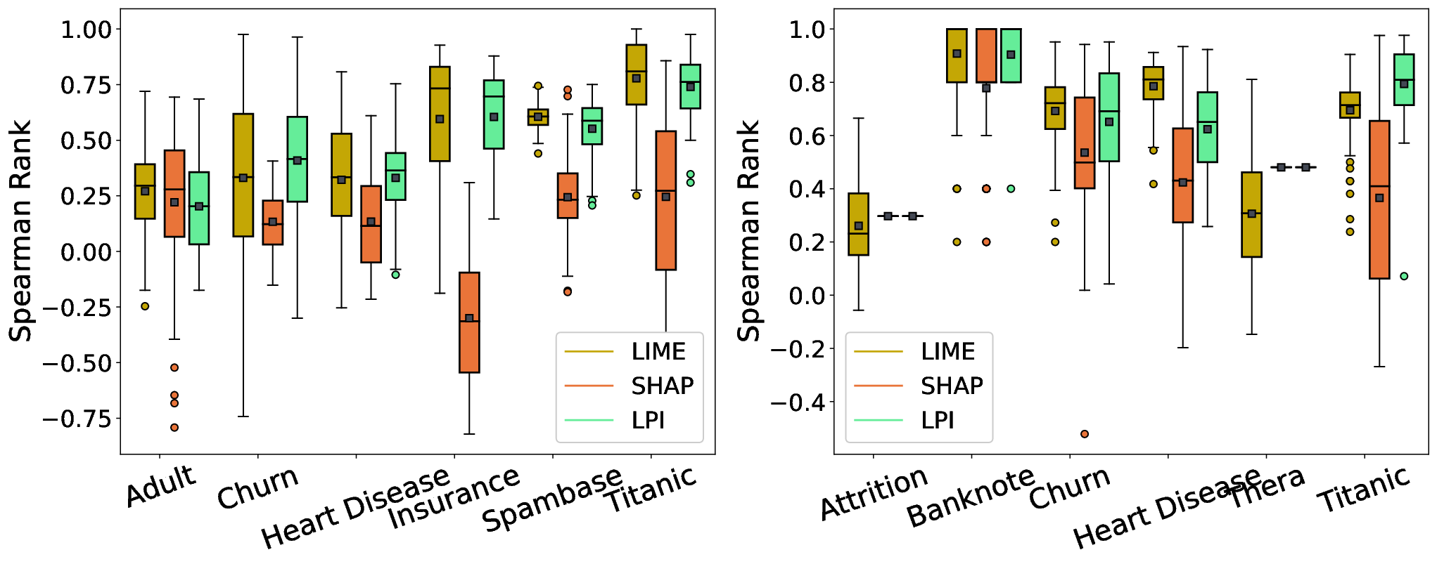
That the performance of the explanation techniques is not constant across different datasets becomes apparent when we observe that the Spearman’s rank correlation can vary to a high degree depending on the data point within each dataset (Figure 3). For several datasets, the standard deviation of the correlation is substantially higher for LIME and SHAP compared to LPI. This means that the explanation techniques to some degree, can produce both highly correlated explanations for some instances of a dataset and weakly correlated or uncorrelated explanations for other instances using exactly the same underlying model. One possible implication of this phenomenon is that local explanation techniques are not able to explain all instances within a dataset accurately. We believe that the local explanation techniques need to develop criteria for cases in which the explanation technique cannot provide an explanation. Based on our knowledge, none of the explanation techniques in this study has such criteria.
Table 2 includes the results of similar experiments with different similarity measures. In the case of Logistic Regression, LIME explanations are most similar to LOR scores when using Cosine and Euclidean similarity. Similar conclusions can be made in the case of naive Bayes. The decrease in the accuracy of LPI explanations can be explained by the fact that, in contrast to LIME and SHAP, LPI’s feature importance scores are non-additive and can therefore not be compared to additive explanations directly in Euclidean space (see Section 3.2 and 3.4.1). The result shows the strong contribution of the choice of a similarity metric on explanation accuracy. The choice of an ideal similarity measure is not an easy task as there is no unified agreement on the optimal measure for explanation accuracy and it is highly dependent on the application scenario (Ghorbani et al. 2019).
| Logistic Regression | naive Bayes | |||||
|---|---|---|---|---|---|---|
| LIME | SHAP | LPI | LIME | SHAP | LPI | |
| Spearman’s Correlation | 0.497 | 0.396 | 0.55 | 0.552 | 0.401 | 0.629 |
| Euclidean Similarity | 0.702 | 0.598 | 0.646 | 0.741 | 0.469 | 0.692 |
| Cosine Similarity | 0.397 | 0.385 | 0.394 | 0.278 | 0.253 | 0.274 |
4.3. Explanation Robustness
In this section, we share the results of empirical experiments on the robustness of LIME, SHAP and LPI explanations when explaining Logistic Regression and naive Bayes on our datasets. Local Lipschitz and and are measures of robustness that are described (see Section 3.5). To recapitulate, a robust explanation technique have relatively low values for Local Lipschitz and and relatively high values for .
In Table 3, the average robustness values are shown across all data sets55 5 The detailed results are reported in Section A.2 in the appendix. , are based on the top-5 important features in the dataset. Local Lipschitz values are based on adding noise from a standard normal distribution with . LPI provides explanations that are more robust in terms of and for both, Logistic Regression and naive Bayes models. For both explained models, SHAP explanations are the most robust in terms of Local Lipschitz measure. We see a different pattern here compared to Table 2. LIME appears to be the least robust explanation technique while simultaneously providing the most accurate explanations in terms of Euclidean and Cosine Similarity. LPI on the other hand seems to be the robust and accurate in terms of Spearman’s Rank Correlation.
| Logistic Regression | naive Bayes | |||||
|---|---|---|---|---|---|---|
| LIME | SHAP | LPI | LIME | SHAP | LPI | |
| 0.108 | 0.086 | 0.122 | 0.096 | 0.117 | 0.257 | |
| 0.038 | 0.049 | 0.033 | 0.084 | 0.082 | 0.061 | |
| 2.17 | 0.172 | 0.191 | 2.621 | 0.441 | 0.896 | |
4.4. Preprocessing effects
As described in Section 4.1, we standardized the numerical features in each dataset before training the logistic regression and naive Bayes models. In this section, we show that the choice of employed preprocessing technique has a substantial effect on the accuracy of the generated explanations. We compare the performances from using three different preprocessing techniques: standardization, robust scaling and minmax (see A.6 for definition).
The first three columns in Table 4 show the average accuracy across all datasets when explaining logistic regression predictions. LIME and SHAP explanations provide the most accurate explanations in many cases when explaining Logistic Regression. The relative performance of explanation techniques can be highly dependent on the preprocessing method used regardless of the measures of similarity used. For example, the difference between performing Minmax or Standard preprocessing can have a substantial and decisive effect in choosing LIME over SHAP in cases where Euclidean or Cosine similarity is used as the similarity metric.
The last three columns of the Table 4 show results for when explaining predictions of naive Bayes models. In this case, the choice of preprocessing technique has less of an effect on the relative performance of the three techniques. LIME and LPI outperform SHAP across all cases.
Since the choice of preprocessing technique has only a very minor effect on the predictive performance of the underlying models across the datasets (see Table 10 in appendix), performance shifts of these models cannot explain the observed differences in explanation accuracy following the choice of preprocessing technique. One possible explanation is that explanation techniques have implicit assumptions on the empirical distributions of features.
| Logistic Regression | naive Bayes | |||||||
|---|---|---|---|---|---|---|---|---|
| Preprocessing | LIME | SHAP | LPI | LIME | SHAP | LPI | ||
| Similarity | Spearman | standard | 0.497 | 0.396 | 0.55 | 0.552 | 0.401 | 0.629 |
| minmax | 0.15 | 0.397 | 0.165 | 0.641 | 0.414 | 0.626 | ||
| robust | 0.315 | 0.618 | 0.303 | 0.596 | 0.401 | 0.628 | ||
| Cosine | Standard | 0.702 | 0.598 | 0.646 | 0.741 | 0.469 | 0.692 | |
| Minmax | 0.276 | 0.348 | 0.17 | 0.82 | 0.478 | 0.691 | ||
| Robust | 0.52 | 0.72 | 0.366 | 0.796 | 0.473 | 0.689 | ||
| Euclidean | Standard | 0.397 | 0.385 | 0.394 | 0.278 | 0.253 | 0.274 | |
| Minmax | 0.325 | 0.387 | 0.336 | 0.282 | 0.251 | 0.273 | ||
| Robust | 0.398 | 0.434 | 0.376 | 0.277 | 0.253 | 0.274 | ||
5. Discussion
Claiming to have derived the true feature importance for a given instance and underlying model, might appear to be unfounded. One could argue that there exist an infinite amount of linear combinations of features that add up to the predicted score, so why would the one presented in this paper be the true decomposition. The beauty of explaining the log odds ratio is that we can extract the exact linear combination based on the model’s parameters for a given instance, i.e., we can extract the only decomposition that the model uses to generate the log odds ratio score.
Another question that might occur to the reader is whether using simple models can tell us anything about the performance of more complex models. It is clear that good performance on simple tasks does not necessarily transfer to good performance on complex tasks. This means that an explanation technique, that has high accuracy according to our method, might not perform well on more complex tasks. The important aspect of using simple tasks however is to have access to a sanity check; if the explanation technique does not work on a simple task, then it is very unlikely that it will have high accuracy on complex tasks. This means that functionally-grounded evaluation methods, such as the one presented here, can be seen as means to make the development of new candidate techniques more efficient; they allow for rejecting some candidate techniques early on. Promising candidates will most likely still need to be qualitatively evaluated in a user-centered context at later stages.
6. Concluding remarks
In this study, we propose an evaluation procedure to directly measure the accuracy of local explanation when explaining the log odds ratio (LOR) scores of logistic regression and naive Bayes models. We showed that in contrast to prediction functions, the log odds ratio functions of these models have intrinsic additive structures. We presented a comparison of explanation techniques based on the extracted true importance scores using Spearman’s rank correlation, Euclidean and Cosine similarity. The results from the extensive empirical investigation showed that the quality of the explanation techniques can depend on the underlying model, the dataset, measure of similarity, which data point is explained, and what pre-processing technique that has been employed. Overall, LPI was observed to often provide more accurate explanations compared to both SHAP and LIME for both logistic regression and naive Bayes models when using Spearman’s rank correlation whereas LIME provided the most accurate explanations when using Euclidean and Cosine similarity.
Based on our empirical experiments, our proposed measure of explanation accuracy is complementary to the functionally-grounded robustness measures. For example, LIME provides relatively low robustness values when explaining Logistic Regression and Naive Bayes models while outperforming LPI and SHAP with regards to explanation accuracy when the similarity metric of choice is Cosine or Euclidean similarity. Based on this, we argue that the notions of explanation robustness and accuracy are orthogonal concepts and should be studied and analyzed separately.
The findings in this study point to several directions for future research. One major open question is how LPI is able to frequently outperform LIME and SHAP despite not even attempting to decompose the predictions into additive terms. Other open questions concern the interplay between the pre-processing technique, underlying model and explanation technique, e.g., how come the choice of pre-processing technique have an effect of the relative performance of the explanation techniques, and why only for one model class?
Another important direction for future research is to extend the proposed evaluation framework to other model classes, e.g., tree models, and explanation types, e.g., rules, as produced by Anchors (Ribeiro et al. 2018). One major challenge here is to derive the true feature importance scores in cases where intrinsic additive structures are not as easily derivable as they are for logistic regression and naive Bayes.
Acknowledgements.
To Robert, for the bagels and explaining CMYK and color spaces.References
- (1)
- Alvarez-Melis and Jaakkola (2018) David Alvarez-Melis and Tommi S Jaakkola. 2018. On the robustness of interpretability methods. ICML Workshop on Human Interpretability in Machine Learning (2018).
- Bishop (2006) Christopher M Bishop. 2006. Pattern recognition. Machine learning 128, 9 (2006).
- Camburu et al. (2019) Oana-Maria Camburu, Eleonora Giunchiglia, Jakob Foerster, Thomas Lukasiewicz, and Phil Blunsom. 2019. Can I trust the explainer? Verifying post-hoc explanatory methods. NeurIPS Workshop on Safety and Robustness in Machine Learning (2019).
- Casalicchio et al. (2018) Giuseppe Casalicchio, Christoph Molnar, and Bernd Bischl. 2018. Visualizing the feature importance for black box models. In Joint European Conference on Machine Learning and Knowledge Discovery in Databases. Springer, 655–670.
- Chen et al. (2018) Jianbo Chen, Le Song, Martin Wainwright, and Michael Jordan. 2018. Learning to explain: An information-theoretic perspective on model interpretation. In International Conference on Machine Learning. PMLR, 883–892.
- Craven and Shavlik (1995) Mark Craven and Jude Shavlik. 1995. Extracting tree-structured representations of trained networks. Advances in neural information processing systems 8 (1995), 24–30.
- Doshi-Velez and Kim (2017) Finale Doshi-Velez and Been Kim. 2017. Towards a rigorous science of interpretable machine learning. arXiv preprint arXiv:1702.08608 (2017).
- Fong and Vedaldi (2017) Ruth C Fong and Andrea Vedaldi. 2017. Interpretable explanations of black boxes by meaningful perturbation. In Proceedings of the IEEE international conference on computer vision. 3429–3437.
- Freitas (2014) Alex A Freitas. 2014. Comprehensible classification models: a position paper. ACM SIGKDD explorations newsletter 15, 1 (2014), 1–10.
- Ghorbani et al. (2019) Amirata Ghorbani, Abubakar Abid, and James Zou. 2019. Interpretation of neural networks is fragile. In Proceedings of the AAAI Conference on Artificial Intelligence, Vol. 33. 3681–3688.
- Hooker et al. (2019) Sara Hooker, Dumitru Erhan, Pieter-Jan Kindermans, and Been Kim. 2019. A benchmark for interpretability methods in deep neural networks. Advances in Neural Information Processing Systems 32 (NeurIPS) (2019).
- Hsieh et al. (2021) Cheng-Yu Hsieh, Chih-Kuan Yeh, Xuanqing Liu, Pradeep Ravikumar, Seungyeon Kim, Sanjiv Kumar, and Cho-Jui Hsieh. 2021. Evaluations and Methods for Explanation through Robustness Analysis. 9th International Conference on Learning Representations, ICLR 2021 (2021).
- Lakkaraju et al. (2020) Himabindu Lakkaraju, Nino Arsov, and Osbert Bastani. 2020. Robust and stable black box explanations. In International Conference on Machine Learning. PMLR, 5628–5638.
- Lipton et al. (2018) Zachary Lipton, Yu-Xiang Wang, and Alexander Smola. 2018. Detecting and correcting for label shift with black box predictors. In International conference on machine learning. PMLR, 3122–3130.
- Lundberg and Lee (2017) Scott Lundberg and Su-In Lee. 2017. A unified approach to interpreting model predictions. Advances in Neural Information Processing Systems 30 (NeruIPS) (2017).
- Montavon et al. (2018) Grégoire Montavon, Wojciech Samek, and Klaus-Robert Müller. 2018. Methods for interpreting and understanding deep neural networks. Digital Signal Processing 73 (2018), 1–15.
- Rahnama and Boström (2019) Amir Hossein Akhavan Rahnama and Henrik Boström. 2019. A study of data and label shift in the LIME framework. Neurip 2019 Workshop on Human-Centric Machine Learning (2019).
- Ribeiro et al. (2016a) Marco Tulio Ribeiro, Sameer Singh, and Carlos Guestrin. 2016a. " Why should i trust you?" Explaining the predictions of any classifier. In Proceedings of the 22nd ACM SIGKDD international conference on knowledge discovery and data mining. 1135–1144.
- Ribeiro et al. (2016b) Marco Tulio Ribeiro, Sameer Singh, and Carlos Guestrin. 2016b. Model-agnostic interpretability of machine learning. ICML Workshop on Human Interpretability in Machine (2016).
- Ribeiro et al. (2018) Marco Tulio Ribeiro, Sameer Singh, and Carlos Guestrin. 2018. Anchors: High-precision model-agnostic explanations. In Proceedings of the AAAI conference on artificial intelligence, Vol. 32.
- Samek et al. (2016) Wojciech Samek, Alexander Binder, Grégoire Montavon, Sebastian Lapuschkin, and Klaus-Robert Müller. 2016. Evaluating the visualization of what a deep neural network has learned. IEEE transactions on neural networks and learning systems 28, 11 (2016), 2660–2673.
- Yang and Kim (2019) Mengjiao Yang and Been Kim. 2019. Benchmarking attribution methods with relative feature importance. Neurip 2019 Workshop on Human-Centric Machine Learning (2019).
- Zeiler and Fergus (2014) Matthew D Zeiler and Rob Fergus. 2014. Visualizing and understanding convolutional networks. In European conference on computer vision. Springer, 818–833.
Appendix A Appendix
A.1. Rank Correlation
Table 5 and 6 show the average Spearman’s rank correlation of explanations with true importance scores when robust and minmax preprocessing is used.
| Model | Logistic Regression | Naïve Bayes | ||||
|---|---|---|---|---|---|---|
| Dataset | LIME | SHAP | LPI | LIME | SHAP | LPI |
| Adult | -0.075 | 0.372 | -0.104 | 0.706 | 0.396 | 0.75 |
| Attrition | 0.329 | 0.413 | 0.215 | 0.232 | 0.297 | 0.297 |
| Audit | 0.486 | 0.971 | 0.579 | 0.466 | 0.364 | 0.522 |
| Banking | 0.257 | 0.601 | 0.006 | 0.486 | 0.088 | 0.847 |
| Banknote | 0.798 | 0.924 | 0.79 | 0.892 | 0.78 | 0.902 |
| Breast Cancer | 0.737 | 0.977 | 0.756 | 0.698 | 0.683 | 0.454 |
| Churn | 0.279 | 0.227 | 0.378 | 0.744 | 0.537 | 0.649 |
| Donors | 0.034 | 0.351 | 0.278 | 0.131 | 0.311 | 0.559 |
| HR | -0.003 | 0.254 | 0.208 | 0.783 | 0.275 | 0.676 |
| Haberman | 0.364 | 0.961 | 0.292 | 0.844 | 0.032 | 0.87 |
| Hattrick | 0.369 | 0.808 | 0.498 | 0.594 | 0.565 | 0.446 |
| Heart Disease | 0.183 | 0.253 | 0.152 | 0.797 | 0.424 | 0.624 |
| Insurance | 0.522 | -0.153 | 0.519 | 0.59 | 0.199 | 0.642 |
| Iris | 0.512 | 0.736 | 0.424 | 0.816 | 0.892 | 0.78 |
| Loan | -0.008 | 0.533 | 0.051 | 0.272 | 0.463 | 0.463 |
| Pima Indians | 0.712 | 0.985 | 0.481 | 0.738 | 0.47 | 0.603 |
| Seismic | 0.195 | 0.801 | 0.107 | 0.786 | 0.202 | 0.726 |
| Spambase | 0.142 | 0.967 | 0.024 | 0.794 | 0.194 | 0.473 |
| Thera | 0.024 | 0.8 | 0.085 | 0.283 | 0.48 | 0.48 |
| Titanic | 0.447 | 0.574 | 0.328 | 0.259 | 0.367 | 0.79 |
| Average | 0.315 | 0.618 | 0.303 | 0.596 | 0.401 | 0.628 |
| Standard Deviation | 0.254 | 0.319 | 0.243 | 0.235 | 0.214 | 0.161 |
| Model | Logistic Regression | Naïve Bayes | ||||
|---|---|---|---|---|---|---|
| Dataset | LIME | SHAP | LPI | LIME | SHAP | LPI |
| Adult | -0.014 | 0.302 | -0.018 | 0.702 | 0.399 | 0.749 |
| Attrition | 0.261 | 0.237 | 0.213 | 0.25 | 0.297 | 0.297 |
| Audit | -0.01 | 0.746 | -0.152 | 0.551 | 0.622 | 0.506 |
| Banking | -0.043 | 0.342 | 0.293 | 0.478 | 0.089 | 0.848 |
| Banknote | 0.708 | 0.708 | 0.684 | 0.894 | 0.786 | 0.902 |
| Breast Cancer | 0.513 | 0.665 | 0.64 | 0.702 | 0.684 | 0.454 |
| Churn | 0.153 | 0.067 | 0.241 | 0.886 | 0.529 | 0.629 |
| Donors | -0.019 | 0.176 | 0.143 | 0.122 | 0.303 | 0.552 |
| HR | 0.083 | 0.283 | 0.341 | 0.786 | 0.276 | 0.675 |
| Haberman | -0.219 | 0.36 | -0.319 | 0.831 | 0.032 | 0.87 |
| Hattrick | 0.273 | 0.44 | 0.329 | 0.614 | 0.563 | 0.449 |
| Heart Disease | 0.107 | 0.17 | 0.031 | 0.802 | 0.423 | 0.623 |
| Insurance | 0.4 | -0.069 | 0.418 | 0.601 | 0.2 | 0.635 |
| Iris | 0.187 | 0.135 | 0.059 | 0.84 | 0.892 | 0.78 |
| Loan | -0.203 | 0.514 | -0.088 | 0.366 | 0.463 | 0.463 |
| Pima Indians | 0.51 | 0.554 | 0.372 | 0.755 | 0.466 | 0.622 |
| Seismic | 0.167 | 0.785 | 0.079 | 0.774 | 0.198 | 0.718 |
| Spambase | -0.141 | 0.883 | -0.265 | 0.795 | 0.193 | 0.468 |
| Thera | -0.212 | 0.519 | -0.09 | 0.255 | 0.48 | 0.48 |
| Titanic | 0.503 | 0.123 | 0.382 | 0.825 | 0.38 | 0.794 |
| Average | 0.15 | 0.397 | 0.165 | 0.641 | 0.414 | 0.626 |
| Standard Deviation | 0.264 | 0.26 | 0.269 | 0.227 | 0.22 | 0.162 |
A.2. Robustness Measures
In this section, the details of measuring robustness for each dataset is presented. Table 7 includes the result of Local Lipschitz measures. As stated earlier, robust explanations have relatively low Local Lipschitz values. Table 8 includes the result of whereas Table 9 shows the result of across all datasets. As stated earlier, larger values of and lower values are desirable for a robust explanation.
| Model | Logistic Regression | Naïve Bayes | ||||
|---|---|---|---|---|---|---|
| Dataset | LIME | SHAP | LPI | LIME | SHAP | LPI |
| Adult | 1.248 | 0.121 | 0.138 | 1.487 | 0.139 | 0.157 |
| Attrition | 0.58 | 0.114 | 0.067 | 0.448 | 0.143 | 0.116 |
| Audit | 5.886 | 0.002 | 0.006 | 5.873 | 0 | 0 |
| Banking | 0.744 | 0.068 | 0.155 | 2.537 | 0.06 | 0.177 |
| Banknote | 1.789 | 0.366 | 0.467 | 0.958 | 0.005 | 0.002 |
| Breast Cancer | 0.576 | 0.169 | 0.176 | 0.55 | 0.181 | 0.227 |
| Churn | 0.808 | 0.086 | 0.092 | 1.612 | 0.109 | 0.121 |
| Donors | 2.856 | 0.013 | 0.023 | 3.389 | 2.537 | 2.525 |
| HR | 5.65 | 0.003 | 0.005 | 6.498 | 0 | 0 |
| Haberman | 2.723 | 0.254 | 0.41 | 0.014 | 2.105 | 5.668 |
| Hattrick | 1.355 | 0.073 | 0.205 | 0.07 | 1.921 | 6.656 |
| Heart Disease | 1.444 | 0.297 | 0.253 | 1.482 | 0.25 | 0.364 |
| Insurance | 2.33 | 0.041 | 0.088 | 6.366 | 0.039 | 0.157 |
| Iris | 0.438 | 0.231 | 0.197 | 1.035 | 0.128 | 0.133 |
| Loan | 2.474 | 0.214 | 0.217 | 2.563 | 0.238 | 0.296 |
| Pima Indians | 1.175 | 0.871 | 0.789 | 0.886 | 0.343 | 0.374 |
| Seismic | 5.202 | 0.263 | 0.253 | 9.003 | 0.28 | 0.432 |
| Spambase | 2.549 | 0.245 | 0.267 | 3.349 | 0.314 | 0.452 |
| Thera | 0.115 | 0.009 | 0.015 | 0.615 | 0.029 | 0.068 |
| Titanic | 3.453 | 0.004 | 0.005 | 3.688 | 0 | 0 |
| Average | 2.17 | 0.172 | 0.191 | 2.621 | 0.441 | 0.896 |
| Standard Deviation | 1.69 | 0.194 | 0.187 | 2.458 | 0.748 | 1.839 |
| Model | Logistic Regression | Naïve Bayes | ||||
|---|---|---|---|---|---|---|
| Dataset | LIME | SHAP | LPI | LIME | SHAP | LPI |
| Adult | 0.062 | 0.059 | 0.064 | 0.067 | 0.058 | 0.067 |
| Attrition | 0.029 | 0.033 | 0.079 | 0.037 | 0.041 | 0.049 |
| Audit | 0.016 | 0.015 | 0.01 | 0.012 | 0.017 | 0.017 |
| Banking | 0.027 | 0.018 | 0.039 | 0.033 | 0.02 | 0.028 |
| Banknote | 0.251 | 0.251 | 0.251 | 0.267 | 0.267 | 0.267 |
| Breast Cancer | 0.096 | 0.095 | 0.106 | 0.105 | 0.104 | 0.108 |
| Churn | 0.027 | 0.01 | 0.025 | 0.054 | 0.025 | 0.058 |
| Donors | 0.235 | 0.174 | 0.248 | 0.447 | 0.391 | 0.602 |
| HR | 0.006 | 0.014 | 0.002 | 0.001 | 0.022 | 0.022 |
| Haberman | 0.292 | 0.059 | 0.289 | 0.006 | 0.513 | 1.7 |
| Hattrick | 0.122 | 0.076 | 0.186 | 0.08 | 0.094 | 1.31 |
| Heart Disease | 0.179 | 0.191 | 0.294 | 0.045 | 0.101 | 0.112 |
| Insurance | 0.029 | 0.015 | 0.033 | 0.028 | 0.029 | 0.019 |
| Iris | 0.071 | 0.071 | 0.071 | 0.06 | 0.06 | 0.06 |
| Loan | 0.15 | 0.121 | 0.15 | 0.185 | 0.153 | 0.174 |
| Pima Indians | 0.294 | 0.294 | 0.294 | 0.222 | 0.222 | 0.222 |
| Seismic | 0.076 | 0.043 | 0.088 | 0.048 | 0.025 | 0.055 |
| Spambase | 0.131 | 0.105 | 0.148 | 0.139 | 0.122 | 0.195 |
| Thera | 0.003 | 0.002 | 0.004 | 0.011 | 0.006 | 0.01 |
| Titanic | 0.06 | 0.069 | 0.062 | 0.064 | 0.07 | 0.07 |
| Average | 0.108 | 0.086 | 0.122 | 0.096 | 0.117 | 0.257 |
| Standard Deviation | 0.094 | 0.081 | 0.101 | 0.108 | 0.132 | 0.441 |
| Model | Logistic Regression | Naïve Bayes | ||||
|---|---|---|---|---|---|---|
| Dataset | LIME | SHAP | LPI | LIME | SHAP | LPI |
| Adult | 0.023 | 0.055 | 0.028 | 0.029 | 0.043 | 0.029 |
| Attrition | 0.111 | 0.11 | 0.033 | 0.019 | 0.008 | 0.042 |
| Audit | 0 | 0.001 | 0 | 0 | 0 | 0 |
| Banking | 0.016 | 0.017 | 0.037 | 0.022 | 0.009 | 0.053 |
| Banknote | 0 | 0 | 0 | 0 | 0 | 0 |
| Breast Cancer | 0.018 | 0.018 | 0.034 | 0.035 | 0.02 | 0.052 |
| Churn | 0.034 | 0.031 | 0.043 | 0.04 | 0.03 | 0.057 |
| Donors | 0.003 | 0.097 | 0.002 | 0.011 | 0.039 | 0.002 |
| HR | 0 | 0.001 | 0 | 0 | 0 | 0 |
| Haberman | 0.272 | 0.182 | 0.255 | 0.61 | 0.61 | 0.02 |
| Hattrick | 0.117 | 0.219 | 0.05 | 0.674 | 0.674 | 0.674 |
| Heart Disease | 0.009 | 0.039 | 0.017 | 0.062 | 0.06 | 0.04 |
| Insurance | 0.02 | 0.011 | 0.022 | 0.023 | 0.004 | 0.089 |
| Iris | 0 | 0 | 0 | 0 | 0 | 0 |
| Loan | 0.011 | 0.096 | 0.014 | 0.016 | 0.072 | 0.015 |
| Pima Indians | 0 | 0 | 0 | 0 | 0 | 0 |
| Seismic | 0.05 | 0.017 | 0.052 | 0.048 | 0.009 | 0.048 |
| Spambase | 0.082 | 0.073 | 0.059 | 0.076 | 0.051 | 0.089 |
| Thera | 0.002 | 0.003 | 0.004 | 0.009 | 0.003 | 0.015 |
| Titanic | 0.001 | 0.007 | 0.001 | 0 | 0 | 0 |
| Average | 0.038 | 0.049 | 0.033 | 0.084 | 0.082 | 0.061 |
| Standard Deviation | 0.064 | 0.062 | 0.055 | 0.188 | 0.188 | 0.143 |
A.3. Accuracy
The test accuracy of Logistic Regression and Naive Bayes models across all datasets is reported in Table 10.
| Pre-processing | Standard | Robust | Minmax | |||
|---|---|---|---|---|---|---|
| dataset | LR | NB | LR | NB | LR | NB |
| Attrition | 1 | 1 | 1 | 1 | 1 | 1 |
| Breast Cancer | 0.965 | 0.916 | 0.965 | 0.916 | 0.965 | 0.916 |
| Pima Indians | 0.802 | 0.766 | 0.776 | 0.766 | 0.802 | 0.766 |
| Banknote | 0.98 | 0.854 | 0.977 | 0.854 | 0.98 | 0.854 |
| Iris | 1 | 1 | 1 | 1 | 1 | 1 |
| Haberman | 0.662 | 0.649 | 0.688 | 0.649 | 0.662 | 0.649 |
| Spambase | 0.921 | 0.808 | 0.886 | 0.808 | 0.921 | 0.809 |
| Adult | 0.841 | 0.805 | 0.835 | 0.805 | 0.841 | 0.801 |
| Heart Disease | 0.829 | 0.829 | 0.829 | 0.829 | 0.829 | 0.829 |
| Churn | 0.805 | 0.826 | 0.806 | 0.826 | 0.805 | 0.826 |
| Hattrick | 1 | 0.939 | 0.995 | 0.939 | 0.998 | 0.939 |
| HR | 0.77 | 0.749 | 0.77 | 0.749 | 0.77 | 0.749 |
| Insurance | 0.987 | 0.953 | 0.987 | 0.953 | 0.987 | 0.953 |
| Audit | 0.99 | 0.974 | 0.974 | 0.969 | 0.995 | 0.974 |
| Loan | 1 | 1 | 1 | 1 | 1 | 1 |
| Donors | 1 | 0.99 | 1 | 0.99 | 1 | 0.988 |
| Seismic | 0.946 | 0.837 | 0.947 | 0.837 | 0.944 | 0.837 |
| Thera | 1 | 1 | 1 | 1 | 1 | 1 |
| Banking | 0.906 | 0.879 | 0.905 | 0.879 | 0.907 | 0.879 |
| Titanic | 0.794 | 0.78 | 0.794 | 0.78 | 0.794 | 0.78 |
A.4. Naïve Bayes example
In this section, we show an example of how LOR scores are extracted for a Naive Bayes model. Let us train a Gaussian Nav̈e Bayes model on the following data and label matrix:
The parameters of the Gaussian distribution for feature 1 and 2 for class 0 are and . Similarly, parameters of the Gaussian distribution for feature 1 and 2 for class 1 are: . For with and , the model predicts . Let , therefore
based on this,
where . While the first feature has an average of -2 for class 0 in the global Gaussian distribution parameters, the contribution of this feature to the LOR of Nav̈e Bayes model for is largely positive, i.e. 11.99. From these two examples, we can see that beside providing true local importance scores, our proposed method can help to quantify the differences between the global and local importance scores in Naive Bayes. Figure 4 shows another example where the extracted LOR scores are compared against different explanations for a test instance in Pima Indians dataset.

A.5. Datasets
Descriptions and access links to all datasets used in this study is available in Table 11.
A.6. Preprocessing techniques
We have included two additional pre-processing techniques including min-max scaling and inter-quartile pre-processing. In inter-quartile pre-processing, median is removed and data is scaled according to the quantile range between the first quartile and the third quartile. For a given random variable , min-max scaling produces as follows: