跳到论文正文
W Papers独立论文阅读器 arXiv:2106.02212 论文正文 计算阅读时间 · 0%
引用这篇论文根据当前论文元数据生成,正式投稿前建议核对。


License: arXiv.org perpetual non-exclusive license
arXiv:2106.02212v2 [cs.LG] 04 Nov 2021

Fuzzy Clustering with Similarity Queries

Wasim Huleihel    Arya Mazumdar    Soumyabrata Pal Thanks: W. Huleihel is with the Department of Electrical Engineering-Systems at Tel Aviv university, Tel Aviv 6997801, Israel (e-mail: wasimh@tauex.tau.ac.il). Thanks: A.Mazumdar is with the Halıcıoğlu Data Science Institute at University of California, San Diego, USA (email: arya@ucsd.edu) Thanks: S. Pal is with the Computer Science Department at the University of Massachusetts Amherst, Amherst, MA 01003, USA (email: spal@cs.umass.edu).
Abstract

The fuzzy or soft kk-means objective is a popular generalization of the well-known kk-means problem, extending the clustering capability of the kk-means to datasets that are uncertain, vague and otherwise hard to cluster. In this paper, we propose a semi-supervised active clustering framework, where the learner is allowed to interact with an oracle (domain expert), asking for the similarity between a certain set of chosen items. We study the query and computational complexities of clustering in this framework. We prove that having a few of such similarity queries enables one to get a polynomial-time approximation algorithm to an otherwise conjecturally NP-hard problem. In particular, we provide algorithms for fuzzy clustering in this setting that ask O⁡(𝗉𝗈𝗅𝗒⁡(k)​log⁡n)O(\mathsf{poly}(k)\log n) similarity queries and run with polynomial-time-complexity, where nn is the number of items. The fuzzy kk-means objective is nonconvex, with kk-means as a special case, and is equivalent to some other generic nonconvex problem such as non-negative matrix factorization. The ubiquitous Lloyd-type algorithms (or alternating minimization algorithm) can get stuck at a local minima. Our results show that by making few similarity queries, the problem becomes easier to solve. Finally, we test our algorithms over real-world datasets, showing their effectiveness in real-world applications.

1 Introduction

The kk-means objective for clustering is perhaps the most ubiquitous of all unsupervised learning paradigms. It is extremely well studied, with Lloyd’s algorithm being the most popular solution method, while the problem in general being NP Hard [11, 7]. A variety of approximate solutions for kk-means exists (such as, [20, 3]).

In recent times, there have been efforts to bring in a flavor of active learning in kk-means clustering; by allowing the learner to make a limited number of carefully chosen label/membership queries [4, 2, 18]. In this setting, the main objective is to show that a polynomial-time solution exists provided that small number of such queries to an oracle is permitted. Note that, an alternative to membership query (i.e., query of the form “does the i𝗍𝗁i^{\mathsf{th}} element belong to the j𝗍𝗁j^{\mathsf{th}} cluster”) is the same-cluster/similarity query (i.e., “do elements ii and jj belong to the same cluster”). Given representatives from each cluster is available, one can simulate any membership query with at most kk same cluster queries. Hence whatever is achievable with membership queries, can be also achieved by same cluster queries by asking at most kk times as many queries [4].

How realistic is to allow the learner to make such label queries, and how realistic is the oracle assumption? It turns out that many clustering tasks, primarily entity-resolution, are being delegated to crowdsourcing models. One can easily assume that the crowd is playing the role of an oracle here. It is natural in these models to assign crowd workers with sub-tasks, which can either be answering the membership query or the same cluster query [5, 49, 50, 38, 23].

Fuzzy kk-means or soft kk-means is a generalized model of the kk-means objective that covers lot more grounds being applicable to dataset where datapoints show affinity to multiple labels, the clustering criteria are vague and data features are unavailable [8]. In fuzzy clustering, instead of an element being part of one fixed cluster, it is assumed that it has a membership value between 00 and 11 to each of the clusters. The objective of the clustering is to recover all of the membership values for each element or datapoint. This relaxation in membership values from {0,1}\{0,1\} to [0,1][0,1] makes the fuzzy kk-means an attractive model for overlapping clusters [52], multilabel classification [30] and numerous other applications such as, pattern recognition [8], computational biology [6], bioinformatics [47], image segmentation [1, 19] and so on.

What is more interesting is that solving fuzzy clustering is equivalent to approximate solution of nonnegative symmetric matrix factorization problems [22]. Given such applications, it is somewhat surprising that the theoretical results known about fuzzy clustering is quite limited. As is even the computational tractability of fuzzy kk-means is only conjecturally known. In fact algorithmic study of fuzzy kk-means algorithm seems to have been only recently started [9, 10, 31].

1.1 Membership vs. Similarity Queries

As mentioned above, in the hard-clustering case, one can simulate any membership query with at most kk same-cluster (or, similarity) queries [4]. In fuzzy clustering, we are given a set of nn vectors (items) in the dd-dimensional Euclidean space, and we are tasked the problem of determining the kk-dimensional membership vector for each of the items. The clustering algorithm has access to the set of vectors, and can also make queries about the underlying soft clustering. As in hard-clustering, these queries can take at least two forms. Specifically, membership queries refer to the existence of a membership-oracle which whenever queried, replies with the membership value of the ithi^{\rm th} item to the jthj^{\rm th} cluster, i.e., the jthj^{\rm th} entry of the ithi^{\rm th} membership vector. One could argue that querying the membership values, and specifically, the existence of such a membership-oracle, is not realistic, and often impractical in real-world settings since it requires knowledge of the relevant clusters. Instead, the similarity query model that takes two or three elements as input and ask “How similar are all these elements?" is much easier to implement in practice. Accordingly, in a similar vein to hard-clustering, we show that membership queries can be simulated by similarity queries, measured by the inner-product between pairs (and triplets) of membership vectors. Finally, as will be explained in more detail, the responses of the oracle or the target solution do not need to correspond to the optimum solution of the fuzzy kk-means objective, but instead need to satisfy a few mild conditions. Accordingly, the target solution can represent noisy/quantized version of the optimum solution of the fuzzy kk-means objective function making our set-up highly practical in crowdsourcing settings.

A natural question that one can ask about fuzzy clustering following the lead of [4] is how many membership/similarity queries one may ask so that the clustering can be efficiently solved with a good approximation of the target solution? In this paper, our main motivation is to answer this rather basic question. It has to be noted that revealing a fractions of labels during clustering algorithm in fuzzy kk-means has been studied with some heuristics in [42], but not only the model was different from ours, a rigorous theoretical study was also lacking in the past literature.

1.2 Our Contributions and Techniques

We design several algorithms and analyze their query and computational complexities. Specifically, the first algorithm we propose works in two phases: in the first phase, we estimate the center of each cluster using non-adaptive queries, and in the second phase we recover the membership of each element to each cluster using the estimated centers obtained in the first phase. We show with this algorithm it is possible to get an approximation of the membership vectors by making only O⁡(poly⁡(k/β)​log⁡n)O({\rm poly}(k/\beta)\log n) queries, where β\beta is ratio of the volume of the smallest cluster to the average volume, informally speaking. Then, we show that by allowing one to ask adaptive/sequential queries in the first phase, the polynomial dependence on β\beta of the query complexity can be further improved. Despite the strong dependency of the query complexity on β\beta, for a large regime of parameters, our query complexity is non-trivial and sublinear in nn. Interestingly, for the special case of k=2k=2, we can completely get rid of the dependency of the query complexity on β\beta, and it suffices to ask O⁡(log2⁡n)O(\log^{2}n) queries only.

For our theoretical results to hold, we make an assumption on the dataset that quantifies the clusterability of the data. We would like to emphasize that our assumption is only needed for deriving the theoretical guarantees; our algorithms are demonstrated to perform well on real-world datasets irrespective of whether our assumption holds or not. The computational complexity of all the algorithms scales as dd times the number of queries.

It is to be noted that the analysis of the aforementioned algorithms are technically much more demanding than solving the analogous query complexity problem for hard kk-means. For the case of hard kk-means, a general principle would be to sample a small set of items and estimate the centre of the largest cluster from the samples (see, [4]). Subsequently all the items closest to the estimated centre can be assigned to it and the cluster can be removed from consideration. One can iterate over this algorithm to find all the clusters. However the size of a cluster is not well-defined in the fuzzy setting; and also it is not possible to assign items to a cluster and remove them from consideration, since they can very well have nonzero memberships to other clusters.

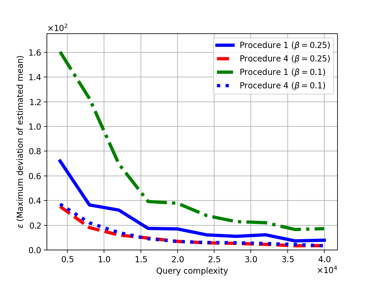
To tackle these difficulties, we have to use more challenging technical tools and analysis methods than the hard kk-means literature. In a nutshell, since at any step of the algorithm we cannot remove items from consideration, we propose sophisticated random sub-sampling algorithms that explore the space of items efficiently. Specifically, having reliable approximations for the centers and memberships of some processed clusters, we partition the space of items into bins that have the same approximated sum of membership weights to unprocessed clusters. Sampling equally from every bin ensures that we obtain enough samples from items which have high membership weight to those clusters which have not yet been approximated. Also, contrary to hard kk-means where a simple (unbiased) empirical mean estimator is used to approximate the means, in the fuzzy setting, we end up with a form of self-normalized importance sampling estimators. While these estimators are biased, we managed to bound their deviations in an elegant way using concentration inequalities. We tested our algorithms over both synthetic and real-world datasets, and illustrate the trade off and effect of different values of β\beta and kk on the estimation error and query complexity.

1.3 Related Work

Clustering with limited label-queries have mostly followed two different lines of works. In the first line of work, queries were used to make the objective based clustering, such as kk-means, polynomial time solvable [4, 2, 18, 12, 13, 14]. The problem being considered here is most closely related to this line of work, albeit, instead of hard kk-means, we focus on a soft objective.

In the second line of work, instead of an objective based clustering, it is assumed that there exists a ground-truth clustering, and by label-querying, one gets a (noisy) answer from an oracle about this ground-truth. The aim of this line of work has been to give statistical-computational guarantees on recovery of the ground truth [36, 37, 35, 2, 15, 46, 43]. The work in this canon that is closest to our problem is [28], where an overlapping clustering groundtruth was considered. At a high level, we also consider overlapping clusters, however, focus on objective-based clustering therein.

It is worth noting that clustering with same cluster, or other label queries, has found connections with and application to correlation clustering [15, 43], community detection [37, 17], heavy-hitters [44] and possibly other areas, that we might have missed. Our problem can be seen as approximately equivalent to non-negative symmetric matrix factorization [40] with limited access to the entries of the factors (via queries) [22].

1.4 Organization

The rest of the paper is organized as follows. In Section 2 we present our model and the learning problem. Then, in Section 3 we present our algorithms and their theoretical guarantees. The main theoretical results can be found in Theorems 1,2,3, followed by several experimental results over both synthetic and real-world datasets. Finally, our conclusion an outlook appear in Section 6. Some technical proofs and discussions are relegated to the appendices.

2 Model Formulation and Background

2.1 The Optimization Problem

We start by describing the hard kk-means problem, and then move forward to the fuzzy kk-means problem (soft clustering). Let 𝒳⊂ℝd{\cal X}\subset\mathbb{R}^{d} be a set of dd-dimensional points, with |𝒳|=n|{\cal X}|=n. We denote this set of vectors by {𝒙i}i=1n\{\boldsymbol{x}_{i}\}_{i=1}^{n}, and assume without loss of generality that 𝒙i∈ℬ⁡(𝟎,𝖱)\boldsymbol{x}_{i}\in{\cal B}(\boldsymbol{0},\mathsf{R}), for any i∈[n]i\in[n], where ℬ⁡(𝒂,𝖱){\cal B}(\boldsymbol{a},\mathsf{R}) is the L2L_{2}-Euclidean ball of radius 𝖱∈ℝ+\mathsf{R}\in\mathbb{R}_{+} centered around 𝒂∈ℝd\boldsymbol{a}\in\mathbb{R}^{d}. Let 𝒞𝒳≜{𝒞1,𝒞2,…,𝒞k}{\cal C}_{{\cal X}}\triangleq\{{\cal C}_{1},{\cal C}_{2},\ldots,{\cal C}_{k}\} be a clustering (or, partition) of 𝒳{\cal X}, where k∈ℕk\in\mathbb{N} is the number of clusters. We say that a clustering 𝒞𝒳{\cal C}_{{\cal X}} is center-based if there exists a set of centers 𝝁≜{𝝁1,𝝁2,…,𝝁k}⊂ℝd\boldsymbol{\mu}\triangleq\{\boldsymbol{\mu}_{1},\boldsymbol{\mu}_{2},\ldots,\boldsymbol{\mu}_{k}\}\subset\mathbb{R}^{d} such that the clustering is induced by the Voronoi diagram over those center points. The objective function of hard kk-means is

𝖩𝗄𝗆​(𝒳,𝝁,𝖴)=∑i=1n∑j=1k𝖴i​j​∥𝒙i−𝝁j∥22,\displaystyle\mathsf{J_{km}}({\cal X},{\mbox{\boldmath$\mu$}},\mathsf{U})=\sum_{i=1}^{n}\sum_{j=1}^{k}\mathsf{U}_{ij}\lVert\boldsymbol{x}_{i}-\boldsymbol{\mu}_{j}\rVert_{2}^{2}, (1)

where 𝖴∈{0,1}n×k\mathsf{U}\in\{0,1\}^{n\times k} is the partition matrix, i.e., the membership weight 𝖴i​j\mathsf{U}_{ij} is 1 if 𝒙i∈𝒞j\boldsymbol{x}_{i}\in{\cal C}_{j}, and 0 otherwise. In hard clustering each data point is assigned exactly to one cluster and every cluster must contain at least one data point. The goal of kk-means is to minimize (1) w.r.t. (𝝁,𝖴)({\mbox{\boldmath$\mu$}},\mathsf{U}).

In soft-clustering there is no partitioning of 𝒳{\cal X}. Instead, we describe the k𝗍𝗁k^{\mathsf{th}} cluster of a fuzzy clustering as a vector of the fractions of points assigned to it by the membership function. In particular, the memberships weights take on real-valued numbers in [0,1][0,1] rather than {0,1}\{0,1\}, as for hard clustering. The fuzzy kk-means problem is defined as follows.

Definition 1 (Fuzzy kk-means).

Let α≥1\alpha\geq 1 and k∈ℕk\in\mathbb{N}. The fuzzy kk-means problem is to find a set of means 𝛍={𝛍ℓ}ℓ∈[k]⊂ℝd{\mbox{\boldmath$\mu$}}=\{{\mbox{\boldmath$\mu$}}_{\ell}\}_{\ell\in[k]}\subset\mathbb{R}^{d} and a membership matrix 𝖴∈[0,1]n×k\mathsf{U}\in[0,1]^{n\times k} minimizing

𝖩𝖿𝗆​(𝒳,𝝁,𝖴)≜∑i=1n∑j=1k𝖴i​jα​∥𝒙i−𝝁j∥22,\displaystyle\mathsf{J_{fm}}({\cal X},{\mbox{\boldmath$\mu$}},\mathsf{U})\triangleq\sum_{i=1}^{n}\sum_{j=1}^{k}\mathsf{U}^{\alpha}_{ij}\lVert\boldsymbol{x}_{i}-{\mbox{\boldmath$\mu$}}_{j}\rVert^{2}_{2}, (2)

subject to ∑j=1k𝖴i​j=1\sum_{j=1}^{k}\mathsf{U}_{ij}=1 and 0<∑i=1n𝖴i​j<n0<\sum_{i=1}^{n}\mathsf{U}_{ij}<n, for all i∈[n]i\in[n] and j∈[k]j\in[k].

The parameter α\alpha is called the fuzzifier, and is not subject to optimization. It can be shown that when α→1\alpha\to 1, the fuzzy kk-means solution coincides with that of the hard kk-means problem. Similarly to the classical kk-means problem, it is easy to optimize the means or memberships of fuzzy kk-means, assuming the other part of the solution is fixed. Specifically, given a set of means 𝝁\mu, it can be shown that the optimal membership weights minimizing the cost in (2) are (see, e.g., [8, Theorem 11.1])

𝖴i​j=[∑ℓ=1k(∥𝒙i−𝝁j∥∥𝒙i−𝝁ℓ∥)2/(α−1)]−1,\displaystyle\mathsf{U}_{ij}=\left[\sum_{\ell=1}^{k}\left(\frac{\lVert\boldsymbol{x}_{i}-\boldsymbol{\mu}_{j}\rVert}{\lVert\boldsymbol{x}_{i}-\boldsymbol{\mu}_{\ell}\rVert}\right)^{2/(\alpha-1)}\right]^{-1}, (3)

for all i∈[n],j∈[k]i\in[n],\;j\in[k]. On the other hand, given a set of membership weights 𝖴\mathsf{U}, the optimal centers are given by

𝝁j=∑i=1n𝖴i​jα​𝒙i∑i=1n𝖴i​jα,\displaystyle\boldsymbol{\mu}_{j}=\frac{\sum_{i=1}^{n}\mathsf{U}_{ij}^{\alpha}\boldsymbol{x}_{i}}{\sum_{i=1}^{n}\mathsf{U}_{ij}^{\alpha}}, (4)

for all i∈[n],j∈[k]i\in[n],\;j\in[k]. Iterating these solutions is known as the Lloyd’s algorithm [32], which provably lands on a local optima. It is well-known, however, that finding the optimal solution (i.e., global minimia) to the kk-means problem is is NP-hard in general [33, 48]. While the same result is unknown for the fuzzy formulation, it is strongly believed to be the case (e.g., [9, 16]).

Finally, although several validity indexes for the performance of fuzzy kk-means solutions have been proposed in the literature (see, e.g., [24, 25]), the Xie–Beni [51] is the most widely used in the literature. This measure is defined as follows11 1 In (5) we divide by n​knk and not just by nn, as in [51], where kk was consider a fixed parameter. If kk is allowed to grow (e.g., with nn), then our definition makes more sense, as in general the numerator in (5) can grow with kk.

𝖷𝖡⁡(𝒳,𝝁,𝖴)≜𝖩𝖿𝗆​(𝒳,𝝁,𝖴)n​k⋅mini≠j⁡∥𝝁i−𝝁j∥22.\displaystyle\mathsf{XB}({\cal X},{\mbox{\boldmath$\mu$}},\mathsf{U})\triangleq\frac{\mathsf{J_{fm}}({\cal X},{\mbox{\boldmath$\mu$}},\mathsf{U})}{nk\cdot\min_{i\neq j}\lVert{\mbox{\boldmath$\mu$}}_{i}-{\mbox{\boldmath$\mu$}}_{j}\rVert_{2}^{2}}. (5)

For the rest of this paper, we denote a clustering by 𝒫≜(𝝁,𝖴){\cal P}\triangleq(\boldsymbol{\mu},\mathsf{U}), and we replace 𝖷𝖡⁡(𝒳,𝝁,𝖴)\mathsf{XB}({\cal X},{\mbox{\boldmath$\mu$}},\mathsf{U}) by 𝖷𝖡⁡(𝒳,𝒫)\mathsf{XB}({\cal X},{\cal P}). Accordingly, the optimal solution to the fuzzy kk-means problem (Defintion 1) is denoted by 𝒫⋆{\cal P}^{\star}. Finally, we say that a clustering 𝒫{\cal P} is consistent center-based if:

  • •

    Given membership weights 𝖴\mathsf{U}, the centers 𝝁\boldsymbol{\mu} are given by (4).

  • •

    The membership weights 𝖴\mathsf{U} are monotone, i.e., if ∥𝒙i−𝝁j∥2≤∥𝒙ℓ−𝝁j∥2\lVert\boldsymbol{x}_{i}-\boldsymbol{\mu}_{j}\rVert_{2}\leq\lVert\boldsymbol{x}_{\ell}-\boldsymbol{\mu}_{j}\rVert_{2} then 𝖴i​j≥𝖴ℓ​j\mathsf{U}_{ij}\geq\mathsf{U}_{\ell j}, for any i,ℓ∈[n]i,\ell\in[n] and j∈[k]j\in[k].

The first condition appears also in [4]. The second condition excludes inconsistent membership weights 𝖴\mathsf{U}. In particular, as is shown in [16], and in Lemma 12 in the appendix, both conditions are satisfied by the optimal solution 𝒫⋆{\cal P}^{\star}, as well as by (4). We would like to clarify that the above assumptions are only required for the theoretical analysis; Our proposed algorithms can be implemented regardless of these assumptions. As is shown in Appendix 5, in real-world applications, our algorithm works well even if these assumptions do not hold.

2.2 Domain Expert/Oracle

Our goal is to construct efficient algorithms with the aid of a domain expert who can give an approximate solution to the fuzzy kk-means problem. Specifically, given a clustering 𝒫{\cal P}, a 𝒫{\cal P}-oracle is a function 𝒪𝒫{\cal O}_{{\cal P}} that answers queries consistent with 𝒫{\cal P}. One can think of such an oracle as a user that has some idea about its desired solution, enough to answer the algorithm’s queries. Importantly, note that as long as 𝒫{\cal P} is a consistent center-based clustering, it need not be the optimal solution 𝒫⋆{\cal P}^{\star} minimizing (2). The algorithm then tries to recover (or, approximate) 𝒫{\cal P} by querying the oracle a small number of times. For hard clustering, the same-cluster query oracle model (i.e., “do elements ii and jj belong to the same cluster") was considered in [4]. Using a certain number of such same-cluster queries and the data points 𝒳{\cal X}, the clustering 𝒫{\cal P} can be found efficiently [4], while finding the optimal solution without the aid of an oracle is NP-hard. For the fuzzy formulation, one can think of analogous oracle models, and in this paper, we focus on the following.

Definition 2 (Membership-Oracle).

A membership query asks the membership weight of an instance 𝐱i\boldsymbol{x}_{i} to a cluster jj, i.e., 𝒪fuzzy​(i,j)=𝖴i​j{\cal O}_{\mathrm{fuzzy}}(i,j)=\mathsf{U}_{ij}.

Basically we ask the oracle for the membership weight of 𝒙i\boldsymbol{x}_{i} to cluster 𝒞j{\cal C}_{j}. Using a certain amount of such queries and the data set 𝒳{\cal X} we would like to approximate the solution for fuzzy kk-means problem. As discussed in the Introduction, one could argue that querying the membership values, and specifically, the existence of such a membership-oracle, is not realistic, and often impractical in real-world settings since it requires knowledge of the relevant clusters. Instead, the following similarity query models are easy to implement in practice.

Definition 3 (Similarity-Oracle).

A fuzzy pairwise similarity query asks the similarity of two distinct instances 𝐱p\boldsymbol{x}_{p} and 𝐱q\boldsymbol{x}_{q} i.e., 𝒪sim​(p,q)=⟨𝖴p,𝖴q⟩{\cal O}_{\mathrm{sim}}(p,q)=\langle\mathsf{U}_{p},\mathsf{U}_{q}\rangle. A fuzzy triplet similarity query asks the similarity of three distinct instances 𝐱p,𝐱q,𝐱r\boldsymbol{x}_{p},\boldsymbol{x}_{q},\boldsymbol{x}_{r}, i.e., 𝒪triplet​(p,q,r)=∑t∈[k]𝖴p​t​𝖴q​t​𝖴r​t{\cal O}_{\mathrm{triplet}}(p,q,r)=\sum_{t\in[k]}\mathsf{U}_{pt}\mathsf{U}_{qt}\mathsf{U}_{rt}.

We show in Appendix D, however, that each membership query can be simulated with a few similarity queries. From a theoretical perspective, membership queries can be simulated with only fuzzy pairwise similarity queries if there exists many pure instances (instances that have a membership weight of 1 to a particular cluster in the dataset), see Lemma 14 in appendix. Unfortunately this strong condition is necessary as well. But it turns out that by using a few triplet similarity queries at the beginning, we can resolve this issue. Specifically, we prove the following result, informally stated, that is interesting in its own right.

Lemma 1 (Membership to Similarity Queries Reduction, Informal).

Suppose there exists an algorithm 𝒜n\mathcal{A}_{n} with time complexity 𝖳n\mathsf{T}_{n} that uses mm membership queries to provide some guaranteed solution of the fuzzy kk-means problem. In that case, under mild conditions on the dataset, the same guarantee can be obtained with O⁡(k3)O(k^{3}) fuzzy triplet similarity queries and O⁡(k​m)O(km) fuzzy pairwise similarity queries, with a time complexity of 𝖳n+O⁡(m​k+k3)\mathsf{T}_{n}+O(mk+k^{3}).

Therefore, we can express everything in terms of the more natural notion of similarity queries and hence, we use membership queries for the rest of the paper to make the representation of our algorithms simpler.

Noisy/Inaccurate Oracle.

Our algorithms work even with inaccuracies in the oracle answer, provided the deviation is small. Under the assumption that such inaccuracies are random, in particular, a repetition algorithm can remedy such errors. Specifically, consider the case where 𝒪fuzzy​(i,j)=𝖴i​j+ζi​j{\cal O}_{\mathrm{fuzzy}}(i,j)=\mathsf{U}_{ij}+\zeta_{ij}, where ζi​j\zeta_{ij} is a zero-mean random variable, and assume the errors to be independent, i.e., the answers are collected from independent crowd-workers. Then, in Appendix C we show how one can convert any “successful" solver for the noiseless problem into a solver for the noisy problem; generally speaking, by repeating the noiseless solver for 𝖳\mathsf{T} consecutive steps using the noisy responses, and then averaging the results to obtain the final estimate. Note that, the technique used to handle the subsequent steps are also applicable to any bounded error. For simplicity of exposition and clarity, we opted to focus on the noiseless setting given in Definition 2.

2.3 Objective and Learning Problem

The goal of the algorithm is to find an approximated clustering that is consistent with the answers given to its queries. We have the following definition.

Definition 4 (Oracle-Based Solver).

Let (𝒳,𝒫)({\cal X},{\cal P}) be a clustering instance. An algorithm 𝒜{\cal A} is called a (ϵ1,ϵ2,𝖰)(\epsilon_{1},\epsilon_{2},\mathsf{Q})-solver if it can approximate 𝒫{\cal P} by having access to 𝒳{\cal X} and making at most 𝖰\mathsf{Q} membership queries to a 𝒫{\cal P}-oracle. Specifically, for any ϵ1,ϵ2>0\epsilon_{1},\epsilon_{2}>0, the algorithm outputs 𝒫^\widehat{{\cal P}} such that maxj∈[k]⁡∥𝛍j−𝛍^j∥2≤ϵ1\max_{j\in[k]}\lVert{\mbox{\boldmath$\mu$}}_{j}-\widehat{{\mbox{\boldmath$\mu$}}}_{j}\rVert_{2}\leq\epsilon_{1} and maxi∈[n],j∈[k]⁡|𝖴i​j−𝖴^i​j|≤ϵ2\max_{i\in[n],j\in[k]}|\mathsf{U}_{ij}-\widehat{\mathsf{U}}_{ij}|\leq\epsilon_{2}. Such an algorithm is a polynomial (ϵ1,ϵ2,𝖰)(\epsilon_{1},\epsilon_{2},\mathsf{Q})-solver if its time-complexity is polynomial in (n,k,ϵ1−1,ϵ2−1)(n,k,\epsilon_{1}^{-1},\epsilon_{2}^{-1}).

We would like to emphasize that we seek an approximate solution rather than exact one. It is important to note 𝖰=O⁡(n​k)\mathsf{Q}=O(nk) membership queries suffice to recover the 𝒫{\cal P}-oracle clustering. Also, with unbounded computational resources one can find the optimal clustering 𝒫⋆{\cal P}^{\star} without any queries. Nonetheless, in this paper, we would like to have a sub-linear dependency of the query complexity on nn and a polynomial dependency of the time complexity on n,kn,k. Having an algorithm such as the one in Definition 4, implies the following guarantee, proved in Appendix A.

Lemma 2.

Let (𝒳,𝒫)({\cal X},{\cal P}) be a clustering instance, and 𝒜{\cal A} be a (ϵ1,ϵ2,𝖰)(\epsilon_{1},\epsilon_{2},\mathsf{Q})-solver. Then,

|𝖷𝖡⁡(𝒳,𝒫)−𝖷𝖡⁡(𝒳,𝒫^)|≤𝖷𝖡⁡(𝒳,𝒫)⋅O⁡(ϵ1)+O⁡(ϵ2)mini≠j⁡∥𝝁i−𝝁j∥22+o⁡(ϵ12+ϵ22mini≠j⁡∥𝝁i−𝝁j∥22).\displaystyle\left|\mathsf{XB}({\cal X},{\cal P})-\mathsf{XB}({\cal X},\widehat{{\cal P}})\right|\leq\frac{\mathsf{XB}({\cal X},{\cal P})\cdot O(\epsilon_{1})+O(\epsilon_{2})}{\min_{i\neq j}\lVert\boldsymbol{\mu}_{i}-\boldsymbol{\mu}_{j}\rVert_{2}^{2}}+o\left(\frac{\epsilon_{1}^{2}+\epsilon_{2}^{2}}{\min_{i\neq j}\lVert\boldsymbol{\mu}_{i}-\boldsymbol{\mu}_{j}\rVert_{2}^{2}}\right). (6)

The lemma above shows that if ϵ1\epsilon_{1} and ϵ2\epsilon_{2} are small enough, then the 𝖷𝖡\mathsf{XB} measure associated with an (ϵ1,ϵ2,𝖰)(\epsilon_{1},\epsilon_{2},\mathsf{Q})-solver is “close" to the 𝖷𝖡\mathsf{XB} measure associated with 𝒫{\cal P}. Note, however, that the r.h.s. of (6) depends inversely on mini≠j⁡∥𝝁i−𝝁j∥22\min_{i\neq j}\lVert\boldsymbol{\mu}_{i}-\boldsymbol{\mu}_{j}\rVert_{2}^{2}. Accordingly, if for some clustering instance (𝒳,𝒫)({\cal X},{\cal P}) this quantity is too small compared to the estimation error, then the difference |𝖷𝖡⁡(𝒳,𝒫)−𝖷𝖡⁡(𝒳,𝒫^)||\mathsf{XB}({\cal X},{\cal P})-\mathsf{XB}({\cal X},\widehat{{\cal P}})| is uncontrolled. This is reasonable since when clusters are “close", the estimation task gets harder.

Finally, we introduce certain notations that will be needed for the presentation of our main results. Given a set of points 𝒳{\cal X} and 𝒗∈ℝd\boldsymbol{v}\in\mathbb{R}^{d}, let π𝒗:[n]→[n]\pi_{\boldsymbol{v}}:[n]\rightarrow[n] be the permutation defined on [n][n] such that

∥𝒗−𝒙π𝒗​(i)∥2≤∥𝒗−𝒙π𝒗​(j)∥2,\displaystyle\lVert\boldsymbol{v}-\boldsymbol{x}_{\pi_{\boldsymbol{v}}(i)}\rVert_{2}\leq\lVert\boldsymbol{v}-\boldsymbol{x}_{\pi_{\boldsymbol{v}}(j)}\rVert_{2}, (7)

for all i<j∈[n]i<j\in[n]. To wit, π𝒗\pi_{\boldsymbol{v}} is the ranking of the elements in 𝒳\mathcal{X} when they are sorted in ascending order w.r.t. to their distance from 𝒗\boldsymbol{v}. Then, we let γ∈ℝ+\gamma\in\mathbb{R}_{+} be the maximum positive number such that for all j∈[k]j\in[k],

π𝝁^=π𝝁j,∀𝝁^∈ℬ⁡(𝝁j,γ).\displaystyle\pi_{\widehat{\boldsymbol{\mu}}}=\pi_{\boldsymbol{\mu}_{j}},\quad\forall\widehat{\boldsymbol{\mu}}\in\mathcal{B}(\boldsymbol{\mu}_{j},\gamma). (8)

Intuitively, if one has reliable estimates for the centers, then the ordering of 𝒳{\cal X} w.r.t. these estimated centers is the same as the ordering w.r.t. the target centers. Next, we define the cluster membership size associated with 𝒫{\cal P} by ∑i∈[n]𝖴i​j\sum_{i\in[n]}\mathsf{U}_{ij}, for all j∈[k]j\in[k], and a parameter β∈ℝ+\beta\in\mathbb{R}_{+} by

β≜minj∈[k]⁡kn⋅∑i∈[n]𝖴i​j.\displaystyle\beta\triangleq\min_{j\in[k]}\;\frac{k}{n}\cdot\sum_{i\in[n]}\mathsf{U}_{ij}. (9)

Accordingly, in terms of β\beta, the minimum cluster membership size is at least β​n/k\beta n/k. Notice that β\beta must be less than unity since ∑i,j𝖴i​j=n\sum_{i,j}\mathsf{U}_{ij}=n, and there must exist at least one cluster whose membership size is at most n/kn/k. We mention that β\beta was introduced in [18] as well.

3 Algorithms and Theoretical Guarantees

In this section we provide our algorithms along with their theoretical guarantees, for the setting described in the previous section. Specifically, we assume that the oracle has a consistent center-based clustering in mind. For this model, we provide two different algorithms; the first is a two-phase algorithm, and the second is a sequential one. Finally, for the special case of k=2k=2, we show an algorithm with significantly improved guarantees.

3.1 Two-Phase Algorithm

We start by providing a non-formal description of our algorithm, whose pseudocode is given in Algorithms 1–3. Specifically, in the first three steps of Algorithm 1 we approximate the centers of all clusters. To that end, we start by sampling at random mm elements from [n][n] with replacement, and denote the obtained samples by 𝒮{\cal S}. The value of mm is specified in Theorem 1 below. Subsequently, we query the membership weights 𝖴i​j\mathsf{U}_{ij}, for all i∈𝒮i\in{\cal S} and j∈[k]j\in[k]. Using these queries, we approximate the center of every cluster using the estimator defined in Step 3 of Algorithm 1. Note that this estimator is the most natural candidate when one knows the membership weights only for a set of sub-sampled elements. Although this Algorithm is quite intuitive, it suffers from the natural drawback that if the size of a particular cluster is small, many samples are needed for a reliable estimate of its center. Algorithm 1 Parallel algorithm for approximating 𝒫{\cal P}. 0:  𝒳\mathcal{X}, 𝒪𝖿𝗎𝗓𝗓𝗒{\cal O}_{\mathsf{fuzzy}}, α\alpha, mm, and η\eta. 0:  An estimate 𝒫^\widehat{{\cal P}}. 1:  Let 𝒮{\cal S} be a set of mm elements sampled at random from [n][n] with replacement. 2:  Query 𝒪𝖿𝗎𝗓𝗓𝗒​(i,j)\mathcal{O}_{\mathsf{fuzzy}}(i,j), ∀i∈𝒮,j∈[k]\forall i\in{\cal S},j\in[k]. 3:  Compute 𝝁^j=∑i∈𝒮𝖴i​jα​𝒙i∑i∈𝒮𝖴i​jα,\widehat{\boldsymbol{\mu}}_{j}=\frac{\sum_{i\in\mathcal{S}}\mathsf{U}_{ij}^{\alpha}\boldsymbol{x}_{i}}{\sum_{i\in\mathcal{S}}\mathsf{U}_{ij}^{\alpha}}, ∀j∈[k]\;\forall j\in[k]. 4:  for j=1,2,…,kj=1,2,\dots,k do 5:    {𝖴^i​j}i=1n←\{\widehat{\mathsf{U}}_{ij}\}_{i=1}^{n}\leftarrowMembership(𝒳,𝝁^j,α,η\mathcal{X},\widehat{\boldsymbol{\mu}}_{j},\alpha,\eta). 6:    𝖴^i​j←𝖴^i​j+1−∑j=1k𝖴^i​jk,∀i∈[n]\widehat{\mathsf{U}}_{ij}\leftarrow\widehat{\mathsf{U}}_{ij}+\frac{1-\sum_{j=1}^{k}\widehat{\mathsf{U}}_{ij}}{k},\;\forall i\in[n]. 7:  end for Algorithm 2 Membership(𝒳,𝝁^j,α,η\mathcal{X},\widehat{\boldsymbol{\mu}}_{j},\alpha,\eta) 0:  𝒳{\cal X}, and 𝒪𝖿𝗎𝗓𝗓𝗒{\cal O}_{\mathsf{fuzzy}}. 0:  An estimate {𝖴^i​j}i=1n\{\widehat{\mathsf{U}}_{ij}\}_{i=1}^{n}. 1:  Find π𝝁^j\pi_{\widehat{\boldsymbol{\mu}}_{j}} w.r.t. 𝒳{\cal X}. 2:  for s=0,1,…,1/ηs=0,1,\dots,1/\eta do 3:    Find ℓs=𝖺𝗋𝗀𝗆𝖺𝗑i∈[n]​𝖴π𝝁^j​(i)​j≥s​η\ell_{s}=\mathsf{argmax}_{i\in[n]}\mathsf{U}_{\pi_{\widehat{\boldsymbol{\mu}}_{j}}(i)j}\geq s\eta using BinarySearch(𝒳,π𝝁^j,s​η\mathcal{X},\pi_{\widehat{\boldsymbol{\mu}}_{j}},s\eta). 4:  end for 5:  for s=0,1,2,…,1/ηs=0,1,2,\dots,1/\eta do 6:    for i=ℓs,ℓs−1,…,,ℓ(s+1)+1i=\ell_{s},\ell_{s}-1,\dots,,\ell_{(s+1)}+1 do 7:    Set 𝖴^π𝝁^j​(i)​j=s​η\widehat{\mathsf{U}}_{\pi_{\widehat{\boldsymbol{\mu}}^{j}}(i)j}=s\eta. 8:    end for 9:  end for

Algorithm 3 BinarySearch(𝒳,π,x\mathcal{X},\pi,x)
0:  𝒪𝖿𝗎𝗓𝗓𝗒{\cal O}_{\mathsf{fuzzy}}.
1:  Set 𝗅𝗈𝗐=1\mathsf{low}=1 and 𝗁𝗂𝗀𝗁=n\mathsf{high}=n.
2:  while 𝗅𝗈𝗐≠𝗁𝗂𝗀𝗁\mathsf{low}\neq\mathsf{high} do
3:    Set 𝗆𝗂𝖽=⌈(𝗅𝗈𝗐+𝗁𝗂𝗀𝗁)/2⌉\mathsf{mid}=\lceil(\mathsf{low}+\mathsf{high})/2\rceil.
4:    Query 𝒪𝖿𝗎𝗓𝗓𝗒​(π​(𝗆𝗂𝖽),j)\mathcal{O}_{\mathsf{fuzzy}}(\pi(\mathsf{mid}),j).
5:    if 𝖴π⁡(𝗆𝗂𝖽)​j≥x\mathsf{U}_{\pi(\mathsf{mid})j}\geq x then
6:    Set 𝗅𝗈𝗐=𝗆𝗂𝖽\mathsf{low}=\mathsf{mid}.
7:    else
8:    Set 𝗁𝗂𝗀𝗁=𝗆𝗂𝖽−1\mathsf{high}=\mathsf{mid}-1.
9:    end if
10:  end while

Next, using the approximated centers, we approximate the membership weights of every element up to a precision of η\eta by using Algorithm 2. To that end, in the first step of this algorithm, we sort the elements of 𝒳{\cal X} in an ascending order according to their distance from the estimated center. Accordingly, if the estimation error of the centers ϵ\epsilon satisfies ϵ≤γ\epsilon\leq\gamma, then (8) implies that the obtained ordering of elements after sorting from the estimated centers is same as the true ordering of the elements obtained by sorting according to distance (in ascending order) from the exact centers (instead of approximated centers). Furthermore, the fact that 𝒫{\cal P} is a consistent center-based clustering implies that for any j∈[k]j\in[k] the membership weights 𝖴π𝝁^j​(i)​j\mathsf{U}_{\pi_{\widehat{\boldsymbol{\mu}}_{j}(i)}j} are non-increasing in ii. Therefore, for any j∈[k]j\in[k] using the binary search in Algorithm 3, we find the maximum index ℓs\ell_{s} such that 𝖴π𝝁^j​(ℓs)​j\mathsf{U}_{\pi_{\widehat{\boldsymbol{\mu}}_{j}(\ell_{s})}j} is larger than s​ηs\eta, for s∈{0,1,…,1/η}s\in\{0,1,\dots,1/\eta\}. This will create an η\eta-spaced grid, and we approximate each membership weight in accordance to the cell it falls into. Specifically, we assign 𝖴^π𝝁^j​(t)​j=s​η\widehat{\mathsf{U}}_{\pi_{\widehat{\boldsymbol{\mu}}_{j}(t)}j}=s\eta, for all t∈[ℓs,ℓs−1,…,ℓs+1+1]t\in[\ell_{s},\ell_{s}-1,\ldots,\ell_{s+1}+1]. Clearly, the estimation error is at most η\eta. Overall, each binary search step takes O⁡(log⁡n)O(\log n) queries, and therefore the total query complexity of this step is O⁡(log⁡n/η)O(\log n/\eta). Finally, Step 6 transforms 𝖴^i​j\widehat{\mathsf{U}}_{ij} to ensure that ∑i=1n𝖴^i​j=1\sum_{i=1}^{n}\widehat{\mathsf{U}}_{ij}=1, for j∈[k]j\in[k]. We have the following result, the detailed proof of which is delegated to Appendix 4.1.

Theorem 1.

Let (𝒳,𝒫)({\cal X},{\cal P}) be a consistent center-based clustering instance, and recall the definitions of γ∈ℝ+\gamma\in\mathbb{R}_{+} and β∈(0,1)\beta\in(0,1) in (8)-(9). Pick ϵ≤γ\epsilon\leq\gamma, η∈(0,1)\eta\in(0,1), and δ∈(0,1)\delta\in(0,1). Take as input to Algorithm 1 m≥(𝖱​kαϵ​βα)4​c​log⁡kδm\geq\left(\frac{\mathsf{R}k^{\alpha}}{\epsilon\beta^{\alpha}}\right)^{4}c\log\frac{k}{\delta}, for some c>0c>0. Then, with probability at least 1−δ1-\delta, Algorithm 1 is (ϵ,η,𝖰)(\epsilon,\eta,\mathsf{Q})-solver using 𝖰=O⁡(𝖱4​k4​α+1(ϵ​βα)4​log⁡kδ+k​log⁡nη)\mathsf{Q}=O\left(\frac{\mathsf{R}^{4}k^{4\alpha+1}}{(\epsilon\beta^{\alpha})^{4}}\log\frac{k}{\delta}+\frac{k\log n}{\eta}\right) membership queries. Furthermore, Algorithm 1 time-complexity is of order O⁡(k​n​log⁡n+d​𝖱4​k4​α+1(ϵ​βα)4​log⁡kδ+k​log⁡nη)O\left(kn\log n+\frac{d\mathsf{R}^{4}k^{4\alpha+1}}{(\epsilon\beta^{\alpha})^{4}}\log\frac{k}{\delta}+\frac{k\log n}{\eta}\right).

Proof Sketch of Theorem 1.

To prove Theorem 1 we first show that with high probability, Steps 1–4 in Algorithm 1 output an ϵ\epsilon-approximation for all centers. To that end, we first show in Lemma 3 that for a given cluster j∈[k]j\in[k], with probability 1−δ1-\delta, ∥𝝁j−𝝁^j∥22≤4​𝖱2𝖸2​cm​log⁡1δ\lVert\boldsymbol{\mu}_{j}-\widehat{\boldsymbol{\mu}}_{j}\rVert^{2}_{2}\leq\frac{4\mathsf{R}^{2}}{\mathsf{Y}^{2}}\sqrt{\frac{c}{m}\log\frac{1}{\delta}}, where 𝖸≜minj∈[k]⁡1n​∑i∈[n]𝖴i​jα\mathsf{Y}\triangleq\min_{j\in[k]}\frac{1}{n}\sum_{i\in[n]}\mathsf{U}_{ij}^{\alpha}. This result follows by noticing that both the numerator and denominator of 𝝁^j\widehat{\boldsymbol{\mu}}_{j} are unbiased estimates of the corresponding numerator and denominator of 𝝁j\boldsymbol{\mu}_{j} in (4). Representing 𝝁^j\widehat{\boldsymbol{\mu}}_{j} as a sum of the true underlying center 𝝁j\boldsymbol{\mu}_{j} and a certain error term, the generalized Hoeffding’s inequality in Lemma 11 implies the above estimation error guarantee. In light of this result, using Hölder’s inequality and the union bound we show in Lemma 5 that ∥𝝁^j−𝝁j∥2≤ϵ\lVert\widehat{\boldsymbol{\mu}}_{j}-\boldsymbol{\mu}_{j}\rVert_{2}\leq\epsilon, for all j∈[k]j\in[k], if mm is as given in Theorem 1. Note that this centers estimation algorithm requires a total of k​mkm membership-oracle queries. Next, conditioned on the above proxy of any given center, we show in Lemma 4 that Algorithm 2 estimates the corresponding membership weights within a certain range of error with high probability. Specifically, for a given cluster jj, we prove that Algorithm 2 outputs 𝖴^i​j\widehat{\mathsf{U}}_{ij}, for i∈[n]i\in[n], such that 0≤𝖴i​j−𝖴^i​j≤η0\leq\mathsf{U}_{ij}-\widehat{\mathsf{U}}_{ij}\leq\eta and 𝖴^i​j∈{0,η,2​η,…,1}\widehat{\mathsf{U}}_{ij}\in\{0,\eta,2\eta,\dots,1\}, ∀i∈[n]\forall i\in[n], using O⁡(log⁡n/η)O\left(\log n/\eta\right) queries to the membership-oracle. Roughly speaking, this result follows from the arguments presented in the paragraph preceding the statement of Theorem 1. Finally, it is evident from the above that the total number of membership-oracle queries is O⁡(k​m+k​log⁡n/η)O(km+k\log n/\eta). ∎

Note that both the query and computational complexities in Theorem 1 exhibit an exponential dependency on the “fuzzifier" α\alpha. As mentioned in Subsection 2.1, this parameter is not subject to optimization and, usually, practitioners pick α=2\alpha=2. Nonetheless, there has been a lot of work on this topic; one notable example is [27] which presents an initial theoretical approach towards the investigation of this question. It seems that the value of α\alpha is influenced by the structure of the dataset, i.e., the number of clusters and the distribution of each cluster. Currently, a definite answer on how to pick α\alpha is unknown. Indeed, since there is no baseline, one cannot decide which value of α\alpha is preferable. Note also that despite the fact that our query complexity naturally depend on α\alpha, it cannot be used to determine the “best" value of α\alpha. Assuming the existence of a ground truth, in Appendix 5 we compare the clustering accuracy for different values of α\alpha on a real-world dataset.

3.2 Sequential Algorithm

As mentioned in the previous subsection, the main drawback faced by Algorithm 1 is its undesirable strong dependency on β\beta. The algorithm proposed in this section remedies this drawback to some extent. The algorithm works as follows. In the first four steps of Algorithm 1, we randomly draw mm samples from [n][n], and query the membership weights that correspond to all these samples. Using these samples we estimate the center of largest cluster t1t_{1}, having the maximal total membership weight ∑i∈𝒮𝖴i​jα\sum_{i\in{\cal S}}\mathsf{U}_{ij}^{\alpha}, among the kk clusters. Corollary 4 in Section 4.2 specifies the number of such elements needed to have a reliable estimate. Then, using this approximated center, we estimate the membership of every element in cluster t1t_{1} using Algorithm 2 such that the estimate is a multiple of η1\eta_{1} and further, the estimate has an additive error of at most η1\eta_{1}, just as we did in the two-phase algorithm. For the rest of the clusters, we follow the sequential algorithm in Steps 5–13 of Algorithm 4, the guarantees of which are characterized in the following result:

Theorem 2.

Let (𝒳,𝒫)({\cal X},{\cal P}) be a consistent center-based clustering instance, and recall the definitions of γ∈ℝ+\gamma\in\mathbb{R}_{+} and β∈(0,1)\beta\in(0,1) in (8)-(9). Take m≥(𝖱​kαϵ)4​c​log⁡2​kδm\geq\left(\frac{\mathsf{R}k^{\alpha}}{\epsilon}\right)^{4}c\log\frac{2k}{\delta}, r≥c​𝖱4​k4​αϵ4​β4​α−4​log⁡4​kη1​δr\geq\frac{c\mathsf{R}^{4}k^{4\alpha}}{\epsilon^{4}\beta^{4\alpha-4}}\log\frac{4k}{\eta_{1}\delta}, for some c>0c>0, and any δ∈(0,1)\delta\in(0,1). Then, with probability at least 1−δ1-\delta, Algorithm 4 is (ϵ,η2,𝖰)(\epsilon,\eta_{2},\mathsf{Q})-solver using 𝖰=O⁡(𝖱4​k4​α+1η1​ϵ4​β4​α−4​log⁡4​kη1​δ+k​log⁡nη1+k​log⁡nη2)\mathsf{Q}=O\left(\frac{\mathsf{R}^{4}k^{4\alpha+1}}{\eta_{1}\epsilon^{4}\beta^{4\alpha-4}}\log\frac{4k}{\eta_{1}\delta}+\frac{k\log n}{\eta_{1}}+\frac{k\log n}{\eta_{2}}\right) membership queries, for any chosen ϵ≤γ\epsilon\leq\gamma and η2≤η1≤1k​(1−βk)\eta_{2}\leq\eta_{1}\leq\frac{1}{k}\left(1-\frac{\beta}{k}\right). Furthermore, Algorithm 4 time-complexity is of order O⁡(d​𝖱4​k4​α+1η1​ϵ4​β4​α−4​log⁡4​kη1​δ+k​log⁡nη1+k​log⁡nη2+k​n​log⁡n)O\left(\frac{d\mathsf{R}^{4}k^{4\alpha+1}}{\eta_{1}\epsilon^{4}\beta^{4\alpha-4}}\log\frac{4k}{\eta_{1}\delta}+\frac{k\log n}{\eta_{1}}+\frac{k\log n}{\eta_{2}}+kn\log n\right).

The proof of Theorem 2 is given in Subsection 4.2, and is based on a technically complicated induction arguments. Below, we provide a short sketch.

Proof Sketch of Theorem 2.

Suppose that we have approximated the means of ℓ≤k\ell\leq k clusters, indexed by 𝒯ℓ≜{t1,t2,…,tℓ}{\cal T}_{\ell}\triangleq\{t_{1},t_{2},\dots,t_{\ell}\}, with an estimation error at most ϵ≤γ\epsilon\leq\gamma, and further approximated the membership weights of every element in 𝒳{\cal X} for all clusters indexed by 𝒯ℓ{\cal T}_{\ell}, up to an additive error η1\eta_{1}. The leftover clusters, indexed by [k]∖𝒯ℓ[k]\setminus{\cal T}_{\ell}, are the unprocessed clusters. The above implies that we can also approximate the sum ∑j∈[ℓ]𝖴i​tj\sum_{j\in[\ell]}\mathsf{U}_{it_{j}}, for each i∈𝒳i\in{\cal X}, up to an additive error ℓ​η1\ell\eta_{1}. Note that, since 𝖴^i​tj\widehat{\mathsf{U}}_{it_{j}} is a multiple of η1\eta_{1} for all j∈[ℓ]j\in[\ell], ∑j∈[ℓ]𝖴^i​tj\sum_{j\in[\ell]}\widehat{\mathsf{U}}_{it_{j}} must also be a multiple of η1\eta_{1}. Subsequently, we partition 𝒳{\cal X} into bins, where the elements in a particular bin have the same approximated sum of membership weights. Formally, let Σ≜{0,1,…,1/η1}\Sigma\triangleq\{0,1,\dots,1/\eta_{1}\}. For each s∈Σs\in\Sigma, we define 𝒳s≜{i∈[n]:∑j∈[ℓ]𝖴^i​tj=s​η1}\mathcal{X}_{s}\triangleq\{i\in[n]:\sum_{j\in[\ell]}\widehat{\mathsf{U}}_{it_{j}}=s\eta_{1}\} to be the s𝗍𝗁s^{\mathsf{th}} bin. Then, in Steps 9-10 of Algorithm 4, we randomly sample min⁡(r,|𝒳s|)\min(r,|{\cal X}_{s}|) elements from each bin with replacement, and denote the resulted sub-sampled set by 𝒴s\mathcal{Y}_{s}. The value of rr is specified in Theorem 2. Sampling equally from every bin ensures that we obtain enough samples from elements which have high membership weight to the unprocessed clusters, i.e., ∑j∈[k]∖[ℓ]𝖴i​tj\sum_{j\in[k]\setminus[\ell]}\mathsf{U}_{it_{j}} is large. Given these sub-sampled sets, we query the membership weights 𝖴i​j\mathsf{U}_{ij}, for all i∈∪s∈Σ𝒴si\in\cup_{s\in\Sigma}{\cal Y}_{s} and j∈[k]∖𝒯ℓj\in[k]\setminus{\cal T}_{\ell}. Using these queries we would like to approximate the center of some unprocessed cluster. We choose the unprocessed cluster having the largest total membership size, weighted by the size of each bin. Mathematically, the index of the (ℓ+1)𝗍𝗁(\ell+1)^{\mathsf{th}} cluster, and its approximated center are given as follows,

tℓ+1\displaystyle t_{\ell+1} ≜𝖺𝗋𝗀𝗆𝖺𝗑j∈[k]∖𝒯ℓ∑s∈Σ|𝒳s|r∑i∈𝒴s𝖴i​jα𝖺𝗇𝖽𝝁^tℓ+1≜∑s∈Σ|𝒳s|r​∑i∈𝒴s𝖴i​tℓ+1α​𝒙i∑s∈Σ|𝒳s|r​∑i∈𝒴s𝖴i​tℓ+1α.\displaystyle\triangleq\underset{j\in[k]\setminus{\cal T}_{\ell}}{\mathsf{argmax}}\;\sum_{s\in\Sigma}\frac{|\mathcal{X}_{s}|}{r}\sum_{i\in\mathcal{Y}_{s}}\mathsf{U}_{ij}^{\alpha}\quad\mathsf{and}\quad\widehat{\boldsymbol{\mu}}_{t_{\ell+1}}\triangleq\frac{\sum_{s\in\Sigma}\frac{|\mathcal{X}_{s}|}{r}\sum_{i\in\mathcal{Y}_{s}}\mathsf{U}_{it_{\ell+1}}^{\alpha}\boldsymbol{x}_{i}}{\sum_{s\in\Sigma}\frac{|\mathcal{X}_{s}|}{r}\sum_{i\in\mathcal{Y}_{s}}\mathsf{U}_{it_{\ell+1}}^{\alpha}}. (10)

We choose the number of samples rr large enough so that the estimation error is less than ϵ\epsilon. The above steps are repeated until all unprocessed clusters are exhausted. Finally, once we have approximated all the centers, we apply Algorithm 2 to approximate the membership weight of every cluster up to an additive error of η2≤η1\eta_{2}\leq\eta_{1}. ∎

Comparing Theorems 1 and 2 we see that the sequential algorithm has a more graceful dependency on β\beta, the size of the smallest cluster. On the other hand, the query complexity of the two-phase algorithm is better in terms of kk (recall that η1≤1/k\eta_{1}\leq 1/k for the sequential algorithm). Note that the query complexity of the sequential algorithm still has some dependency on β\beta. This stems from the fact that we estimate the membership weights up to a precision of η1\eta_{1}, which might be too large if there exists a cluster jj such that maxi∈[n]⁡𝖴i​j≤η1\max_{i\in[n]}\mathsf{U}_{ij}\leq\eta_{1}. Accordingly, in this case, all elements will fall into a single bin in the partition, leading to the same drawback the two-phase algorithm suffers from.

Algorithm 4 Sequential algorithm for approximating 𝒫{\cal P}.
0:  𝒳\mathcal{X}, 𝒪𝖿𝗎𝗓𝗓𝗒{\cal O}_{\mathsf{fuzzy}}, α\alpha, mm, rr, η1\eta_{1}, and η2\eta_{2}.
0:  An estimate 𝒫^\widehat{{\cal P}}.
1:  Let 𝒮{\cal S} be a set of mm elements sampled at random from [n][n] with replacement.
2:  Query 𝒪𝖿𝗎𝗓𝗓𝗒​(i,j),∀i∈𝒮,j∈[k]\mathcal{O}_{\mathsf{fuzzy}}(i,j),\;\forall i\in{\cal S},j\in[k].
3:  t1=𝖺𝗋𝗀𝗆𝖺𝗑j∈[k]​∑i∈𝒮𝖴i​jα.t_{1}=\mathsf{argmax}_{j\in[k]}\sum_{i\in\mathcal{S}}\mathsf{U}_{ij}^{\alpha}.
4:  Compute 𝝁^t1=∑i∈𝒮𝖴i​t1α​𝒙i∑i∈𝒮𝖴i​t1α\widehat{\boldsymbol{\mu}}_{t_{1}}=\frac{\sum_{i\in\mathcal{S}}\mathsf{U}_{it_{1}}^{\alpha}\boldsymbol{x}_{i}}{\sum_{i\in\mathcal{S}}\mathsf{U}_{it_{1}}^{\alpha}}.
5:  for ℓ=1,2,…,k−1\ell=1,2,\dots,k-1 do
6:    {𝖴^i,ℓ}i=1n←\{\widehat{\mathsf{U}}_{i,\ell}\}_{i=1}^{n}\leftarrowMembership(𝒳,𝝁^tℓ,α,η1\mathcal{X},\widehat{\boldsymbol{\mu}}_{t_{\ell}},\alpha,\eta_{1}).
7:    Set 𝒳s≜{i∈[n]:∑j∈[ℓ]𝖴^i​tj=s​η1}\mathcal{X}_{s}\triangleq\{i\in[n]:\sum_{j\in[\ell]}\widehat{\mathsf{U}}_{it_{j}}=s\eta_{1}\} for s∈{0,1,…,1/η1}s\in\{0,1,\dots,1/\eta_{1}\}.
8:    for s=0,1,…,1/η1s=0,1,\dots,1/\eta_{1} do
9:    Let 𝒴s{\cal Y}_{s} be a set of min⁡(r,|𝒳s|)\min(r,|{\cal X}_{s}|) elements sampled at random from 𝒳s\mathcal{X}_{s} with replacement.
10:    end for
11:    Compute tℓ+1t_{\ell+1} using (10).
12:    Compute 𝝁^tℓ+1\widehat{\boldsymbol{\mu}}_{t_{\ell+1}} using (10).
13:  end for
14:  for j=1,2,…,kj=1,2,\dots,k do
15:    {𝖴^i​j}i=1n←\{\widehat{\mathsf{U}}_{ij}\}_{i=1}^{n}\leftarrowMembership(𝒳,𝝁^j,α,η2\mathcal{X},\widehat{\boldsymbol{\mu}}_{j},\alpha,\eta_{2}).
16:    𝖴^i​j←𝖴^i​j+1−∑j=1k𝖴^i​jk,∀i∈[n]\widehat{\mathsf{U}}_{ij}\leftarrow\widehat{\mathsf{U}}_{ij}+\frac{1-\sum_{j=1}^{k}\widehat{\mathsf{U}}_{ij}}{k},\;\forall i\in[n].
17:  end for

3.3 The Special Case of Two Clusters

While the sequential algorithm proposed in the previous subsection exhibits graceful dependency of the query complexity on β\beta, it is still unclear to what extent this dependency can be reduced. Interestingly, it turns out that for the special case of two clusters k=2k=2, we can devise an algorithm whose query complexity is completely independent of β\beta. The proof of the following result is given in Subsection 4.3.

Theorem 3.

Let (𝒳,𝒫)({\cal X},{\cal P}) be a consistent center-based clustering instance, recall the definition of γ∈ℝ+\gamma\in\mathbb{R}_{+} in (8), and let k=2k=2. Then, with probability at least 1−δ1-\delta, Algorithm 5 with m=O⁡((𝖱ϵ)4​log⁡4δ)m=O\left(\Big(\frac{\mathsf{R}}{\epsilon}\Big)^{4}\log\frac{4}{\delta}\right) and r=O⁡(𝖱4ϵ4​log⁡2η​δ)r=O\left(\frac{\mathsf{R}^{4}}{\epsilon^{4}}\log\frac{2}{\eta\delta}\right) is a (ϵ,η,𝖰)(\epsilon,\eta,\mathsf{Q})-solver using

𝖰=O⁡(𝖱4​log⁡n​log⁡(1/η​δ)ϵ4+log2⁡n+log⁡nη)\mathsf{Q}=O\left(\frac{\mathsf{R}^{4}\log n\log(1/\eta\delta)}{\epsilon^{4}}+\log^{2}n+\frac{\log n}{\eta}\right)

membership queries, for any chosen ϵ≤γ,δ∈(0,1)\epsilon\leq\gamma,\;\delta\in(0,1) and η>0\eta>0. Furthermore, Algorithm 5 time-complexity is of order O⁡(n​log⁡n+d​𝖱4​log⁡n​log⁡(1/η​δ)ϵ4+log2⁡n+log⁡nη)O\left(n\log n+\frac{d\mathsf{R}^{4}\log n\log(1/\eta\delta)}{\epsilon^{4}}+\log^{2}n+\frac{\log n}{\eta}\right).

Algorithm 5 Sequential algorithm for approximating 𝒫{\cal P} with two clusters
0:  𝒳{\cal X}, 𝒪𝖿𝗎𝗓𝗓𝗒\mathcal{O}_{\mathsf{fuzzy}}, α\alpha, mm, rr, and η\eta.
1:  Let 𝒮{\cal S} be a set of mm elements sampled at random from [n][n] with replacement.
2:  Query 𝒪𝖿𝗎𝗓𝗓𝗒​(i,j)\mathcal{O}_{\mathsf{fuzzy}}(i,j) and store 𝖴i​j\mathsf{U}_{ij} for all j∈{1,2}j\in\{1,2\}.
3:  Choose t1=𝖺𝗋𝗀𝗆𝖺𝗑j∈{1,2}​∑i∈𝒮𝖴i​jα.t_{1}=\mathsf{argmax}_{j\in\{1,2\}}\sum_{i\in\mathcal{S}}\mathsf{U}_{ij}^{\alpha}.
4:  Compute estimator 𝝁^t1=∑i∈𝒮𝖴i​t1α​𝒙i∑i∈𝒮𝖴i​t1α\widehat{\boldsymbol{\mu}}_{t_{1}}=\frac{\sum_{i\in\mathcal{S}}\mathsf{U}_{it_{1}}^{\alpha}\boldsymbol{x}_{i}}{\sum_{i\in\mathcal{S}}\mathsf{U}_{it_{1}}^{\alpha}}.
5:  Obtain 𝒫1,𝒫2,𝒳1,𝒳2,…,𝒳q\mathcal{P}_{1},\mathcal{P}_{2},\mathcal{X}_{1},\mathcal{X}_{2},\dots,\mathcal{X}_{q} and 𝖴^i​t2\widehat{\mathsf{U}}_{it_{2}} for all i∈[n]i\in[n] using Membership2(𝒳,𝝁^t1,α\mathcal{X},\widehat{\boldsymbol{\mu}}_{t_{1}},\alpha)
6:  for q=1,2,3,…,3​log⁡nq=1,2,3,\dots,3\log n do
7:   Let 𝒴q\mathcal{Y}_{q} be a set of rr elements sampled at random from 𝒳q\mathcal{X}_{q} with replacement.
8:   Query 𝒪𝖿𝗎𝗓𝗓𝗒​(i,t2)\mathcal{O}_{\mathsf{fuzzy}}(i,t_{2}) to obtain 𝖴i​t2\mathsf{U}_{it_{2}} for all i∈𝒴qi\in\mathcal{Y}_{q}
9:  end for
10:  Let 𝒬\mathcal{Q} be a set of rr elements sampled at random from 𝒫1\mathcal{P}_{1} with replacement.
11:  Query 𝒪𝖿𝗎𝗓𝗓𝗒​(i,t2)\mathcal{O}_{\mathsf{fuzzy}}(i,t_{2}) to obtain 𝖴i​t2\mathsf{U}_{it_{2}} for all i∈𝒬i\in\mathcal{Q}.
12:  Compute 𝝁^t2\widehat{\boldsymbol{\mu}}_{t_{2}} in (88).
13:  for j=1,2j=1,2 do
14:   Run Algorithm Membership(𝒳,𝝁^j,α,η,j\mathcal{X},\widehat{\boldsymbol{\mu}}_{j},\alpha,\eta,j) to update 𝖴^i​j\widehat{\mathsf{U}}_{ij} for all i∈[n]i\in[n].
15:  end for
16:  Return 𝝁^j\widehat{\boldsymbol{\mu}}_{j} for all j∈{1,2}j\in\{1,2\} and 𝖴^i​j\widehat{\mathsf{U}}_{ij} for all i∈[n],j∈{1,2}i\in[n],j\in\{1,2\}.

We now explain the main ideas behind Algorithm 5. First, let 𝒮{\cal S} be a set of mm elements sampled from [n][n] with replacement. Denote by t1∈{1,2}t_{1}\in\{1,2\} the index of the larger cluster and t2∈{1,2}t_{2}\in\{1,2\} the index of the smaller cluster, i.e., ∑i∈𝒮𝖴i​t1α>∑i∈𝒮𝖴i​t2α\sum_{i\in{\cal S}}\mathsf{U}_{it_{1}}^{\alpha}>\sum_{i\in{\cal S}}\mathsf{U}_{it_{2}}^{\alpha}. The algorithm works as follows. We start by computing an estimate 𝝁^t1\widehat{\boldsymbol{\mu}}_{t_{1}} for the center of the largest cluster t1t_{1}. Corollary 4 shows that O⁡((𝖱/ϵ)4​log⁡(4/δ))O\left((\mathsf{R}/\epsilon)^{4}\log(4/\delta)\right) membership queries are needed to guarantee that ∥𝝁^t1−𝝁t1∥2≤ϵ\lVert\widehat{\boldsymbol{\mu}}_{t_{1}}-\boldsymbol{\mu}_{t_{1}}\rVert_{2}\leq\epsilon. Now, the main novelty in Algorithm 5 is a non-trivial querying scheme used to estimate the memberships of the second cluster, 𝖴i​t2\mathsf{U}_{it_{2}}, for all i∈[n]i\in[n], using the center estimated for the first cluster t1t_{1}. Note that for the special case of two clusters, querying 𝖴i​t1\mathsf{U}_{it_{1}} reveals 𝖴i​t2\mathsf{U}_{it_{2}} since 𝖴i​t1+𝖴i​t2=1\mathsf{U}_{it_{1}}+\mathsf{U}_{it_{2}}=1. While, in the sequential algorithm, we always approximated the membership weights using bins of fixed size η1\eta_{1}, here, we will approximate 𝖴i​t2\mathsf{U}_{it_{2}} with bins whose size is data-dependent. The reason for using variable bin sizes rather than fixed size bins is that with the latter we might ask for many redundant membership queries simply because many bins might be empty. Accordingly, by adaptively choosing the bin size for approximating the membership weights of the smaller cluster t2t_{2}, while querying membership weights to the larger cluster t1t_{1}, allows us to get around this issue completely; this results in a theoretical guarantee that is completely independent of β\beta.

We now describe Algorithm 6 used to estimate the membership weights of cluster t2t_{2}. We start by sorting 𝒳{\cal X} in ascending order according to their distance from 𝝁^t1\widehat{\boldsymbol{\mu}}_{t_{1}}, and initialize η1=𝖴π𝝁^t1​(n)​t2\eta_{1}=\mathsf{U}_{\pi_{\widehat{\boldsymbol{\mu}}_{t_{1}}}(n)t_{2}} and pη1≜np_{\eta_{1}}\triangleq n. To wit, η1\eta_{1} is the membership of the element farthest from 𝝁^t1\widehat{\boldsymbol{\mu}}_{t_{1}} to the smaller cluster t2t_{2}. For each q∈={2,3​…,3​log⁡n}q\in=\{2,3\dots,3\log n\}, we set ηq=ηq−1/2\eta_{q}=\eta_{q-1}/2, and then perform binary search to find pηq′=𝖺𝗋𝗀𝗆𝗂𝗇j∈[n]𝟙[𝖴π𝝁^t1​(j)​t2≥ηq]p^{\prime}_{\eta_{q}}=\mathsf{argmin}_{j\in[n]}\mathds{1}[\mathsf{U}_{\pi_{\widehat{\boldsymbol{\mu}}_{t_{1}}}(j)t_{2}}\geq\eta_{q}]. Here, we should think of pηq′p^{\prime}_{\eta_{q}} to be the index for which 𝒙π𝝁^t1​(pηq′)\boldsymbol{x}_{\pi_{\widehat{\boldsymbol{\mu}}_{t_{1}}}(p^{\prime}_{\eta_{q}})} is the element closest from 𝝁^t1\widehat{\boldsymbol{\mu}}_{t_{1}}, such that its membership to the smaller cluster t2t_{2} is at least ηq\eta_{q}. Now, if |pηq′−pηq−1|≥log⁡n|p^{\prime}_{\eta_{q}}-p_{\eta_{q-1}}|\geq\log n, we keep ηq\eta_{q} unchanged, set pηq=pηq′p_{\eta_{q}}=p^{\prime}_{\eta_{q}}, and put all elements which are closer to 𝝁^t1\widehat{\boldsymbol{\mu}}_{t_{1}} than 𝒙π𝝁^t1​(pηq−1)\boldsymbol{x}_{\pi_{\widehat{\boldsymbol{\mu}}_{t_{1}}}(p_{\eta_{q-1}})}, but farther than 𝒙π𝝁^t1​(pηq)\boldsymbol{x}_{\pi_{\widehat{\boldsymbol{\mu}}_{t_{1}}}(p_{\eta_{q}})} into a single bin. Notice that each such bin contains at least log⁡n\log n elements by definition. However, if pηq′p^{\prime}_{\eta_{q}} is the same as pηq−1p_{\eta_{q-1}}, then the membership queries in the latter binary search to compute pηq′p^{\prime}_{\eta_{q}} is wasteful. In order to fix this issue, we check if there are a sufficient number (at least log⁡n\log n) of elements between pηq′p^{\prime}_{\eta_{q}} and pηq−1p_{\eta_{q-1}}. If there are not, then we set pηqp_{\eta_{q}} such that the above condition is satisfied. More formally, if |pηq′−pηq−1|≤log⁡n|p^{\prime}_{\eta_{q}}-p_{\eta_{q-1}}|\leq\log n we update pηq=min⁡(0,pηq−1−1−log⁡n)p_{\eta_{q}}=\min(0,p_{\eta_{q-1}}-1-\log n) and ηq=𝖴π𝝁^t1​(pηq)​t2\eta_{q}=\mathsf{U}_{\pi_{\widehat{\boldsymbol{\mu}}_{t_{1}}}(p_{\eta_{q}})t_{2}}. In other words, we set pηqp_{\eta_{q}} such that there at least log⁡n\log n elements between pηqp_{\eta_{q}} and pηq−1p_{\eta_{q-1}}, and accordingly, we set ηq\eta_{q} to be the membership of π𝝁^t1​(pηq)\pi_{\widehat{\boldsymbol{\mu}}_{t_{1}}}(p_{\eta_{q}}) to the cluster t2t_{2}. Subsequently, we query 𝖴i​t2\mathsf{U}_{it_{2}} for every element that is closer to 𝝁^t1\widehat{\boldsymbol{\mu}}_{t_{1}} than 𝒙π𝝁^t1​(pηq−1)\boldsymbol{x}_{\pi_{\widehat{\boldsymbol{\mu}}_{t_{1}}}(p_{\eta_{q-1}})} but farther than 𝒙π𝝁^t1​(pηq)\boldsymbol{x}_{\pi_{\widehat{\boldsymbol{\mu}}_{t_{1}}}(p_{\eta_{q}})}. In this case, we call these elements special elements, since we query every one of them. We will assume that all these special elements between 𝒙π𝝁^t1​(pηq−1)\boldsymbol{x}_{\pi_{\widehat{\boldsymbol{\mu}}_{t_{1}}}(p_{\eta_{q-1}})} and 𝒙π𝝁^t1​(pηq)\boldsymbol{x}_{\pi_{\widehat{\boldsymbol{\mu}}_{t_{1}}}(p_{\eta_{q}})} are assigned a single bin.

Algorithm 6 Membership2(𝒳,𝝁^t1,α\mathcal{X},\widehat{\boldsymbol{\mu}}_{t_{1}},\alpha) Estimate the memberships 𝖴i​t2\mathsf{U}_{it_{2}} for all i∈[n]i\in[n] given an estimated mean 𝝁^t1\widehat{\boldsymbol{\mu}}_{t_{1}}
0:  𝒪𝖿𝗎𝗓𝗓𝗒\mathcal{O}_{\mathsf{fuzzy}}.
1:  Sort the elements 𝒙1,𝒙2,…,𝒙n\boldsymbol{x}_{1},\boldsymbol{x}_{2},\dots,\boldsymbol{x}_{n} in ascending order according to ∥𝒙i−𝝁^t1∥2\lVert\boldsymbol{x}_{i}-\widehat{\boldsymbol{\mu}}_{t_{1}}\rVert_{2}. Denote the resultant permutation of [n][n] corresponding to the sorted elements by π𝝁^t1\pi_{\widehat{\boldsymbol{\mu}}_{t_{1}}}.
2:  Set η1≜1−𝖴π𝝁^t1​(n)​t1andpη1≜n\eta_{1}\triangleq 1-\mathsf{U}_{\pi_{\widehat{\boldsymbol{\mu}}_{t_{1}}}(n)t_{1}}\quad\text{and}\quad p_{\eta_{1}}\triangleq n.
3:  Query 𝒪𝖿𝗎𝗓𝗓𝗒​(π𝝁^t1​(n),t1)\mathcal{O}_{\mathsf{fuzzy}}(\pi_{\widehat{\boldsymbol{\mu}}_{t_{1}}}(n),t_{1}) to obtain 𝖴π𝝁^t1​(n)​t1\mathsf{U}_{\pi_{\widehat{\boldsymbol{\mu}}_{t_{1}}}(n)t_{1}}. Set 𝖴π𝝁^t1​(n),t2=1−𝖴π𝝁^t1​(n)​t1\mathsf{U}_{\pi_{\widehat{\boldsymbol{\mu}}_{t_{1}}}(n),t_{2}}=1-\mathsf{U}_{\pi_{\widehat{\boldsymbol{\mu}}_{t_{1}}}(n)t_{1}}.
4:  Initialize 𝒫1,𝒫2=ϕ\mathcal{P}_{1},\mathcal{P}_{2}=\phi
5:  for q=2,3,…,3​log⁡nq=2,3,\dots,3\log n do
6:   Initialize 𝒳q=ϕ\mathcal{X}_{q}=\phi and set ηq=ηq−12\eta_{q}=\frac{\eta_{q-1}}{2}
7:   Find pηq′=𝖺𝗋𝗀𝗆𝗂𝗇i∈[n]​𝖴π𝝁^t1​(i),t2≥ηqp^{\prime}_{\eta_{q}}=\mathsf{argmin}_{i\in[n]}\mathsf{U}_{\pi_{\widehat{\boldsymbol{\mu}}_{t_{1}}}(i),t_{2}}\geq\eta_{q} using BinarySearch2(𝒳,π𝝁^t1,ηq\mathcal{X},\pi_{\widehat{\boldsymbol{\mu}}_{t_{1}}},\eta_{q}).
8:   if |pηq′−pηq−1|≥log⁡n|p^{\prime}_{\eta_{q}}-p_{\eta_{q-1}}|\geq\log n then
9:    Set pηq=pηq′p_{\eta_{q}}=p^{\prime}_{\eta_{q}}
10:    for i=pηq,pηq+1,…,pηq−1−1i=p_{\eta_{q}},p_{\eta_{q}}+1,\dots,p_{\eta_{q-1}}-1 do
11:     Set 𝒳q=𝒳q∪π𝝁^t1​(i)\mathcal{X}_{q}=\mathcal{X}_{q}\cup\pi_{\widehat{\boldsymbol{\mu}}_{t_{1}}}(i) and set 𝖴^π𝝁^t1​(i),t2=1−𝖴π𝝁^t1​(pηq)​t1\widehat{\mathsf{U}}_{\pi_{\widehat{\boldsymbol{\mu}}_{t_{1}}}(i),t_{2}}=1-\mathsf{U}_{\pi_{\widehat{\boldsymbol{\mu}}_{t_{1}}}(p_{\eta_{q}})t_{1}}
12:    end for
13:   else
14:    Query 𝒪𝖿𝗎𝗓𝗓𝗒​(π𝝁^t1​(min⁡(0,pηq−1−log⁡n−1)),t1)\mathcal{O}_{\mathsf{fuzzy}}(\pi_{\widehat{\boldsymbol{\mu}}_{t_{1}}}(\min(0,p_{\eta_{q-1}}-\log n-1)),t_{1}) and obtain the membership 𝖴π𝝁^t1​(min⁡(0,pηq−1−log⁡n−1)),t1\mathsf{U}_{\pi_{\widehat{\boldsymbol{\mu}}_{t_{1}}}(\min(0,p_{\eta_{q-1}}-\log n-1)),t_{1}}.
15:    Set ηq=𝖴π𝝁^t1​(min⁡(0,pηq−1−log⁡n−1)),t2\eta_{q}=\mathsf{U}_{\pi_{\widehat{\boldsymbol{\mu}}_{t_{1}}}(\min(0,p_{\eta_{q-1}}-\log n-1)),t_{2}} and pηq=min⁡(0,pηq−1−1−log⁡n)p_{\eta_{q}}=\min(0,p_{\eta_{q-1}}-1-\log n).
16:    for i=pηq,pηq+1,…,pηq−1−1i=p_{\eta_{q}},p_{\eta_{q}}+1,\dots,p_{\eta_{q-1}}-1 do
17:     Query 𝒪𝖿𝗎𝗓𝗓𝗒​(π𝝁^t1​(i),t1)\mathcal{O}_{\mathsf{fuzzy}}(\pi_{\widehat{\boldsymbol{\mu}}_{t_{1}}}(i),t_{1}) to obtain 𝖴π𝝁^t1​(i)​t1\mathsf{U}_{\pi_{\widehat{\boldsymbol{\mu}}_{t_{1}}}(i)t_{1}}.
18:     Set 𝖴^π𝝁^t1​(i),t2=1−𝖴π𝝁^t1​(i)​t1\widehat{\mathsf{U}}_{\pi_{\widehat{\boldsymbol{\mu}}_{t_{1}}}(i),t_{2}}=1-\mathsf{U}_{\pi_{\widehat{\boldsymbol{\mu}}_{t_{1}}}(i)t_{1}} and set 𝒳q′=𝒳q′∪π𝝁^t1​(i)\mathcal{X}^{\prime}_{q}=\mathcal{X}^{\prime}_{q}\cup\pi_{\widehat{\boldsymbol{\mu}}_{t_{1}}}(i)
19:    end for
20:   end if
21:  end for
22:  for i=0,1,…,η3​log⁡n−1i=0,1,\dots,\eta_{3\log n}-1 do
23:   Set 𝖴^π𝝁^t1​(i),t2=0\widehat{\mathsf{U}}_{\pi_{\widehat{\boldsymbol{\mu}}_{t_{1}}}(i),t_{2}}=0 and set 𝒫1=𝒫1∪π𝝁^t1​(i)\mathcal{P}_{1}=\mathcal{P}_{1}\cup\pi_{\widehat{\boldsymbol{\mu}}_{t_{1}}}(i)
24:  end for
25:  Set 𝒫2=∪q𝒳′q\mathcal{P}_{2}=\cup_{q}\mathcal{X}^{\prime}_{q}.
26:  Return 𝒫1,𝒫2,𝒳1,𝒳2,…,𝒳q\mathcal{P}_{1},\mathcal{P}_{2},\mathcal{X}_{1},\mathcal{X}_{2},\dots,\mathcal{X}_{q} and 𝖴^i​t2\widehat{\mathsf{U}}_{it_{2}} for all i∈[n]i\in[n].
Algorithm 7 BinarySearch2(𝒳,π,x\mathcal{X},\pi,x): Search for the minimum index ii such that 1−𝖴π⁡(i)​t1≥x1-\mathsf{U}_{\pi(i)t_{1}}\geq x
0:  𝒪𝖿𝗎𝗓𝗓𝗒\mathcal{O}_{\mathsf{fuzzy}}.
1:  Set 𝗅𝗈𝗐=1\mathsf{low}=1 and 𝗁𝗂𝗀𝗁=n\mathsf{high}=n.
2:  while 𝗅𝗈𝗐≠𝗁𝗂𝗀𝗁\mathsf{low}\neq\mathsf{high} do
3:   Set 𝗆𝗂𝖽=⌊(𝗅𝗈𝗐+𝗁𝗂𝗀𝗁)/2⌋\mathsf{mid}=\lfloor(\mathsf{low}+\mathsf{high})/2\rfloor.
4:   Query 𝒪𝖿𝗎𝗓𝗓𝗒​(π⁡(𝗆𝗂𝖽)​t1)\mathcal{O}_{\mathsf{fuzzy}}(\pi(\mathsf{mid})t_{1}) to obtain 𝖴π⁡(𝗆𝗂𝖽)​t1\mathsf{U}_{\pi(\mathsf{mid})t_{1}}.
5:   if 𝖴π⁡(𝗆𝗂𝖽)​t1≥1−x\mathsf{U}_{\pi(\mathsf{mid})t_{1}}\geq 1-x then
6:    Set 𝗅𝗈𝗐=𝗆𝗂𝖽+1\mathsf{low}=\mathsf{mid}+1
7:   else
8:    Set 𝗁𝗂𝗀𝗁=𝗆𝗂𝖽\mathsf{high}=\mathsf{mid}
9:   end if
10:  end while
11:  Return 𝗅𝗈𝗐\mathsf{low}.

To resolve the edge case, we put all those elements which are closer to 𝝁^t1\widehat{\boldsymbol{\mu}}_{t_{1}} than 𝒙π𝝁^t1​(pη3​log⁡n)\boldsymbol{x}_{\pi_{\widehat{\boldsymbol{\mu}}_{t_{1}}}(p_{\eta_{3\log n}})} into a separate bin. Let gg be the total number of bins formed by this algorithm, and say 𝒳j\mathcal{X}_{j} is the j𝗍𝗁j^{\mathsf{th}} bin formed by this method that does not contain any special elements. Let 𝒫\mathcal{P} be the set of all special elements. Notice that the number of bins gg is at most 1+3​log⁡n1+3\log n, and the number of special elements is at most 3​log2​n3\log^{2}n (since each bin can contain at most log⁡n\log n special elements). Moreover, for any bin 𝒳j\mathcal{X}_{j} not containing any special elements, we can show that maxi∈𝒳j⁡𝖴i​t2≤2​mini∈𝒳j​𝖴i​t2\max_{i\in\mathcal{X}_{j}}\mathsf{U}_{it_{2}}\leq 2\min_{i\in\mathcal{X}_{j}}\mathsf{U}_{it_{2}}, which should be contrasted with the guarantee we have for the sequential algorithm, i.e., for a particular bin 𝒳j\mathcal{X}_{j}, |maxi∈𝒳j⁡𝖴i​t2−mini∈𝒳j⁡𝖴i​t2|≤η1|\max_{i\in\mathcal{X}_{j}}\mathsf{U}_{it_{2}}-\min_{i\in\mathcal{X}_{j}}\mathsf{U}_{it_{2}}|\leq\eta_{1}. Finally, we again sub-sample rr elements from each such bin 𝒳j\mathcal{X}_{j} with replacement, and denote the resulting subset by 𝒴j\mathcal{Y}_{j}. We approximate the center of the second cluster by

𝝁^t2=∑j|𝒳j|r​∑i∈𝒴j𝖴i​t2α​𝒙i+∑i∈𝒫𝖴i​t2α​𝒙i∑j|𝒳j|r​∑i∈𝒴j𝖴i​t2α+∑i∈𝒫𝖴i​t2α,\displaystyle\widehat{\boldsymbol{\mu}}_{t_{2}}=\frac{\sum_{j}\frac{|\mathcal{X}_{j}|}{r}\sum_{i\in\mathcal{Y}_{j}}\mathsf{U}_{it_{2}}^{\alpha}\boldsymbol{x}_{i}+\sum_{i\in\mathcal{P}}\mathsf{U}_{it_{2}}^{\alpha}\boldsymbol{x}_{i}}{\sum_{j}\frac{|\mathcal{X}_{j}|}{r}\sum_{i\in\mathcal{Y}_{j}}\mathsf{U}_{it_{2}}^{\alpha}+\sum_{i\in\mathcal{P}}\mathsf{U}_{it_{2}}^{\alpha}}, (11)

and show that the required rr is independent of the cluster size.

4 Proofs

4.1 Proof of Theorem 1

To prove Theorem 1 we will establish some preliminary results.

4.1.1 Auxiliary Lemmata

We start by analyzing the performance of Algorithm 8, which estimates the center of a given cluster using a set of randomly sampled elements. Note that this algorithm is used as a sub-routine of Algorithm 1.

Algorithm 8 Algorithm for estimating the mean 𝝁j\boldsymbol{\mu}_{j} for any j∈[k]j\in[k].
0:  𝒳{\cal X}, 𝒪𝖿𝗎𝗓𝗓𝗒{\cal O}_{\mathsf{fuzzy}}, α\alpha, and mm.
0:  𝝁^j\widehat{\boldsymbol{\mu}}_{j}
1:  Initialize 𝒮←ϕ\mathcal{S}\leftarrow\phi.
2:  for s=1,2,…,ms=1,2,\dots,m do
3:   Sample ii uniformly at random from [n][n] and update 𝒮←𝒮∪{i}\mathcal{S}\leftarrow\mathcal{S}\cup\{i\}.
4:   Query 𝒪𝖿𝗎𝗓𝗓𝗒​(i,j)\mathcal{O}_{\mathsf{fuzzy}}(i,j).
5:  end for
6:  Compute 𝝁^j=∑i∈𝒮𝖴i​jα​𝒙i∑i∈𝒮𝖴i​jα\widehat{\boldsymbol{\mu}}_{j}=\frac{\sum_{i\in\mathcal{S}}\mathsf{U}_{ij}^{\alpha}\boldsymbol{x}_{i}}{\sum_{i\in\mathcal{S}}\mathsf{U}_{ij}^{\alpha}}.
Lemma 3 (Estimate of mean using uniform sampling).

Let (𝒳,𝒫)({\cal X},{\cal P}) be a consistent center-based clustering instance, and let δ∈(0,1)\delta\in(0,1). With probability at least 1−δ1-\delta, Algorithm 8 outputs an estimate 𝛍^j\widehat{\boldsymbol{\mu}}_{j} such that

∥𝝁j−𝝁^j∥22≤4​𝖱2𝖸2​cm​log⁡1δ,\displaystyle\lVert\boldsymbol{\mu}_{j}-\widehat{\boldsymbol{\mu}}_{j}\rVert^{2}_{2}\leq\frac{4\mathsf{R}^{2}}{\mathsf{Y}^{2}}\sqrt{\frac{c}{m}\log\frac{1}{\delta}}, (12)

where 𝖸≜minj∈[k]⁡1n​∑i∈[n]𝖴i​jα\mathsf{Y}\triangleq\min_{j\in[k]}\frac{1}{n}\sum_{i\in[n]}\mathsf{U}_{ij}^{\alpha}, and c>0c>0 is some absolute constant.

Proof of Lemma 3.

First, note that

𝝁^j=∑i∈𝒮𝖴i​jα​𝒙i∑i∈𝒮𝖴i​jα=(1/m)​∑i∈𝒮𝖴i​jα​𝒙i(1/m)​∑i∈𝒮𝖴i​jα≜𝝀¯𝒙𝖸¯.\displaystyle\widehat{\boldsymbol{\mu}}_{j}=\frac{\sum_{i\in\mathcal{S}}\mathsf{U}_{ij}^{\alpha}\boldsymbol{x}_{i}}{\sum_{i\in\mathcal{S}}\mathsf{U}_{ij}^{\alpha}}=\frac{(1/m)\sum_{i\in\mathcal{S}}\mathsf{U}_{ij}^{\alpha}\boldsymbol{x}_{i}}{(1/m)\sum_{i\in\mathcal{S}}\mathsf{U}_{ij}^{\alpha}}\triangleq\frac{\bar{\boldsymbol{\lambda}}_{\boldsymbol{x}}}{\bar{\mathsf{Y}}}. (13)

Recall that the true mean of the j𝗍𝗁j^{\mathsf{th}} cluster is

𝝁j=∑i∈[n]𝖴i​jα​𝒙i∑i∈[n]𝖴i​jα=(1/n)​∑i∈[n]𝖴i​jα​𝒙i(1/n)​∑i∈[n]𝖴i​jα≜𝝀𝒙𝖸.\displaystyle\boldsymbol{\mu}_{j}=\frac{\sum_{i\in[n]}\mathsf{U}_{ij}^{\alpha}\boldsymbol{x}_{i}}{\sum_{i\in[n]}\mathsf{U}_{ij}^{\alpha}}=\frac{(1/n)\sum_{i\in[n]}\mathsf{U}_{ij}^{\alpha}\boldsymbol{x}_{i}}{(1/n)\sum_{i\in[n]}\mathsf{U}_{ij}^{\alpha}}\triangleq\frac{\boldsymbol{\lambda}_{\boldsymbol{x}}}{\mathsf{Y}}. (14)

It is clear that 𝝀¯𝒙\bar{\boldsymbol{\lambda}}_{\boldsymbol{x}} and 𝖸¯\bar{\mathsf{Y}} are an unbiased estimators of 𝝀𝒙\boldsymbol{\lambda}_{\boldsymbol{x}} and 𝖸\mathsf{Y}, respectively. Now, note that we can write 𝝀¯𝒙\bar{\boldsymbol{\lambda}}_{\boldsymbol{x}} as an average of mm i.i.d random variables 𝒙¯ip=𝖴ip​jα​𝒙ip\bar{\boldsymbol{x}}_{i_{p}}=\mathsf{U}_{i_{p}j}^{\alpha}\boldsymbol{x}_{i_{p}}, where ipi_{p} is sampled uniformly at random from [n][n], and included to the set 𝒮\mathcal{S} in the third step of Algorithm 8 as the p𝗍𝗁p^{\mathsf{th}} sample. Similarly, 𝖸¯\bar{\mathsf{Y}} can also be written as the average of mm i.i.d random variables 𝖸¯ip=𝖴ip​jα\bar{\mathsf{Y}}_{i_{p}}=\mathsf{U}_{i_{p}j}^{\alpha}. Further, notice that 𝔼​𝒙¯ip=𝝀𝒙\mathbb{E}\bar{\boldsymbol{x}}_{i_{p}}=\boldsymbol{\lambda}_{\boldsymbol{x}}, ∥𝒙¯ip∥2≤𝖱\lVert\bar{\boldsymbol{x}}_{i_{p}}\rVert_{2}\leq\mathsf{R}, and similarly, 𝔼​𝖸¯ip=𝖸\mathbb{E}\bar{\mathsf{Y}}_{i_{p}}=\mathsf{Y}, and |𝖸¯i,p|≤1\left|\bar{\mathsf{Y}}_{i,p}\right|\leq 1, for all p∈{1,2,…,m}p\in\{1,2,\dots,m\}. Next, note that

𝝁^j\displaystyle\widehat{\boldsymbol{\mu}}_{j} =𝝀¯𝒙𝖸¯=𝝁𝒙𝖸+𝝀¯𝒙−𝝀𝒙𝖸+𝝀¯𝒙𝖸¯​𝖸−𝖸¯𝖸.\displaystyle=\frac{\bar{\boldsymbol{\lambda}}_{\boldsymbol{x}}}{\bar{\mathsf{Y}}}=\frac{{\boldsymbol{\mu}}_{\boldsymbol{x}}}{{\mathsf{Y}}}+\frac{\bar{\boldsymbol{\lambda}}_{\boldsymbol{x}}-\boldsymbol{\lambda}_{\boldsymbol{x}}}{\mathsf{Y}}+\frac{\bar{\boldsymbol{\lambda}}_{\boldsymbol{x}}}{\bar{\mathsf{Y}}}\frac{\mathsf{Y}-\bar{\mathsf{Y}}}{\mathsf{Y}}. (15)

Thus, using the triangle inequality we get

∥𝝁^j−𝝁j∥2≤∥𝝀¯𝒙−𝝀𝒙𝖸∥2+∥𝝀¯𝒙𝖸¯​𝖸−𝖸¯𝖸∥2≤∥𝝀¯𝒙−𝝀𝒙𝖸∥2+𝖱​∥𝖸¯−𝖸𝖸∥2,\displaystyle\lVert\widehat{\boldsymbol{\mu}}_{j}-\boldsymbol{\mu}_{j}\rVert_{2}\leq\lVert\frac{\bar{\boldsymbol{\lambda}}_{\boldsymbol{x}}-\boldsymbol{\lambda}_{\boldsymbol{x}}}{\mathsf{Y}}\rVert_{2}+\lVert\frac{\bar{\boldsymbol{\lambda}}_{\boldsymbol{x}}}{\bar{\mathsf{Y}}}\frac{\mathsf{Y}-\bar{\mathsf{Y}}}{\mathsf{Y}}\rVert_{2}\leq\lVert\frac{\bar{\boldsymbol{\lambda}}_{\boldsymbol{x}}-\boldsymbol{\lambda}_{\boldsymbol{x}}}{\mathsf{Y}}\rVert_{2}+\mathsf{R}\lVert\frac{\bar{\mathsf{Y}}-\mathsf{Y}}{\mathsf{Y}}\rVert_{2}, (16)

where in the last inequality we have used the fact that ∥𝝁^j∥2=∥𝝀¯𝒙/𝖸¯∥2≤𝖱\lVert\widehat{\boldsymbol{\mu}}_{j}\rVert_{2}=\lVert\bar{\boldsymbol{\lambda}}_{\boldsymbol{x}}/\bar{\mathsf{Y}}\rVert_{2}\leq\mathsf{R}. Then, the generalized Hoeffding’s inequality in Lemma 11, implies that with probability at least 1−δ1-\delta,

∥𝝀¯𝒙−𝝀𝒙∥22≤𝖱2​cm​log⁡1δ,\displaystyle\lVert\bar{\boldsymbol{\lambda}}_{\boldsymbol{x}}-\boldsymbol{\lambda}_{\boldsymbol{x}}\rVert_{2}^{2}\leq\mathsf{R}^{2}\sqrt{\frac{c}{m}\log\frac{1}{\delta}}, (17)

for some c>0c>0, and thus,

∥𝝁^j−𝝁j∥22≤4​𝖱2𝖸2​cm​log⁡1δ.\displaystyle\lVert\widehat{\boldsymbol{\mu}}_{j}-\boldsymbol{\mu}_{j}\rVert_{2}^{2}\leq\frac{4\mathsf{R}^{2}}{\mathsf{Y}^{2}}\sqrt{\frac{c}{m}\log\frac{1}{\delta}}. (18)

which concludes the proof. ∎

The following lemma shows that if for a given cluster jj we have been able to approximate its center well enough, then Algorithm 2 computes good estimates of the corresponding membership weights with high probability.

Lemma 4 (Estimate of membership given estimated center).

Let (𝒳,𝒫)({\cal X},{\cal P}) be a consistent center-based clustering instance, and recall the definition of γ∈ℝ+\gamma\in\mathbb{R}_{+} in (8). Assume that for any j∈[k]j\in[k], there exists an estimator 𝛍^j\widehat{\boldsymbol{\mu}}_{j} such that ∥𝛍j−𝛍^j∥2≤ϵ\lVert\boldsymbol{\mu}_{j}-\widehat{\boldsymbol{\mu}}_{j}\rVert_{2}\leq\epsilon with ϵ≤γ\epsilon\leq\gamma. Then, Algorithm 2 outputs 𝖴^i​j\widehat{\mathsf{U}}_{ij}, for i∈[n]i\in[n], such that

0≤𝖴i​j−𝖴^i​j≤η,𝖴^i​j∈{0,η,2​η,…,1},∀i∈[n],\displaystyle 0\leq\mathsf{U}_{ij}-\widehat{\mathsf{U}}_{ij}\leq\eta,\quad\widehat{\mathsf{U}}_{ij}\in\{0,\eta,2\eta,\dots,1\},\quad\forall i\in[n], (19)

for some η∈ℝ+\eta\in\mathbb{R}_{+}, using 𝖰=O⁡(log⁡n/η)\mathsf{Q}=O\left(\log n/\eta\right) queries to the membership-oracle.

Proof of Lemma 4.

First, note that since 𝒫{\cal P} is a consistent center-based clustering, we have

𝖴π𝝁j​(i1)​j≥𝖴π𝝁j​(i2)​jifi1<i2,i1,i2∈[n].\displaystyle\mathsf{U}_{\pi_{\boldsymbol{\mu}_{j}}(i_{1})j}\geq\mathsf{U}_{\pi_{\boldsymbol{\mu}_{j}}(i_{2})j}\quad\text{if}\quad i_{1}<i_{2},i_{1},i_{2}\in[n]. (20)

Indeed, when the elements of 𝒳{\cal X} are sorted in ascending order according to their distance from 𝝁j\boldsymbol{\mu}_{j}, if 𝒙u1\boldsymbol{x}_{u_{1}} is closer to 𝝁j\boldsymbol{\mu}_{j} than it is to 𝒙u2\boldsymbol{x}_{u_{2}}, then 𝖴u1​j>𝖴u2​j\mathsf{U}_{u_{1}j}>\mathsf{U}_{u_{2}j}. Also, since ∥𝝁j−𝝁^j∥2≤ϵ≤γ\lVert\boldsymbol{\mu}_{j}-\widehat{\boldsymbol{\mu}}_{j}\rVert_{2}\leq\epsilon\leq\gamma, using (8), this ordering remains the same. Therefore, sorting the elements in 𝒳\mathcal{X} in ascending order from 𝝁^j\widehat{\boldsymbol{\mu}}_{j} as in the first step of Algorithm 2 gives the same ordering with respect to the true mean. Now, given η∈ℝ+\eta\in\mathbb{R}_{+}, for each s∈{0,1,2,…,1/η}s\in\{0,1,2,\dots,1/\eta\}, in the third step of Algorithm 2 we binary search to find an index ℓs\ell_{s} such that

ℓs=𝖺𝗋𝗀𝗆𝖺𝗑i∈[n]​𝖴π𝝁^j​(i)​j≥s​η.\displaystyle\ell_{s}=\underset{i\in[n]}{\mathsf{argmax}}\;\mathsf{U}_{\pi_{\widehat{\boldsymbol{\mu}}_{j}}(i)j}\geq s\eta. (21)

This is done by using O⁡(log⁡n/η)O(\log n/\eta) membership-oracle queries. Finally, in the last three steps of Algorithm 2, for each s∈{0,1,2,…,1/η}s\in\{0,1,2,\dots,1/\eta\}, and for i∈{ℓs,ℓs−1,…,ℓ(s+1)+1}i\in\{\ell_{s},\ell_{s}-1,\dots,\ell_{(s+1)}+1\}, we assign 𝖴^π𝝁^j​(i)​j=s​η\widehat{\mathsf{U}}_{\pi_{\widehat{\boldsymbol{\mu}}_{j}}(i)j}=s\eta. It is then clear that the estimated memberships satisfy (19), which concludes the proof. ∎

Using the above lemmas we obtain the following.

Lemma 5 (Estimate all means).

Let (𝒳,𝒫)({\cal X},{\cal P}) be a consistent center-based clustering instance, recall the definition of β∈(0,1)\beta\in(0,1) in (9), and let δ∈(0,1)\delta\in(0,1). Then, with probability at least 1−δ1-\delta, Algorithm 8 outputs 𝛍^j\widehat{\boldsymbol{\mu}}_{j} such that ∥𝛍^j−𝛍j∥2≤ϵ\lVert\widehat{\boldsymbol{\mu}}_{j}-\boldsymbol{\mu}_{j}\rVert_{2}\leq\epsilon, for all j∈[k]j\in[k], if m≥(𝖱​kαϵ​βα)4​c​log⁡kδm\geq\left(\frac{\mathsf{R}k^{\alpha}}{\epsilon\beta^{\alpha}}\right)^{4}c\log\frac{k}{\delta}, for some c>0c>0.

Proof.

Using (9) and Hölder’s inequality, for any j∈[k]j\in[k] we have,

(∑i∈[n]𝖴i​jα)1/α​(∑i∈[n]1α/(α−1))(α−1)/α≥∑i∈[n]𝖴i​j≥β​nk,\displaystyle\left(\sum_{i\in[n]}\mathsf{U}_{ij}^{\alpha}\right)^{1/\alpha}\left(\sum_{i\in[n]}1^{\alpha/(\alpha-1)}\right)^{(\alpha-1)/\alpha}\geq\sum_{i\in[n]}\mathsf{U}_{ij}\geq\frac{\beta n}{k}, (22)

which implies that

(∑i∈[n]𝖴i​jα)1/α≥β​nk​n(α−1)/α=β​n1/αk,\displaystyle\left(\sum_{i\in[n]}\mathsf{U}_{ij}^{\alpha}\right)^{1/\alpha}\geq\frac{\beta n}{kn^{(\alpha-1)/\alpha}}=\frac{\beta n^{1/\alpha}}{k}, (23)

and thus

∑i∈[n]𝖴i​jα≥n​βαkα.\displaystyle\sum_{i\in[n]}\mathsf{U}_{ij}^{\alpha}\geq\frac{n\beta^{\alpha}}{k^{\alpha}}. (24)

Therefore,

𝖸=minj∈[k]⁡∑i∈[n]𝖴i​jαn≥(βk)α\displaystyle\mathsf{Y}=\min_{j\in[k]}\frac{\sum_{i\in[n]}\mathsf{U}_{ij}^{\alpha}}{n}\geq\Big(\frac{\beta}{k}\Big)^{\alpha}

Now, using Lemma 3 and the last result, taking a union bound over all j∈[k]j\in[k], we get

∥𝝁^j−𝝁j∥2≤2​𝖱​kαβα​(cm​log⁡1δ′)1/4≤ϵ.\displaystyle\lVert\widehat{\boldsymbol{\mu}}_{j}-\boldsymbol{\mu}_{j}\rVert_{2}\leq\frac{2\mathsf{R}k^{\alpha}}{\beta^{\alpha}}\Big(\frac{c}{m}\log\frac{1}{\delta^{\prime}}\Big)^{1/4}\leq\epsilon. (25)

with probability 1−k​δ′1-k\delta^{\prime}. Rearranging terms and substituting δ=k​δ′\delta=k\delta^{\prime}, we get the proof of the lemma. ∎

4.1.2 Proof of Theorem 1

We are now in a position to prove Theorem 1. Using Lemma 5, we can conclude that by taking m≥(𝖱​kαϵ​βα)4​c​log⁡kδm\geq\left(\frac{\mathsf{R}k^{\alpha}}{\epsilon\beta^{\alpha}}\right)^{4}c\log\frac{k}{\delta} in Algorithm 1, which would require k​mkm membership-oracle queries, we get ∥𝝁^j−𝝁j∥2≤ϵ\lVert\widehat{\boldsymbol{\mu}}_{j}-\boldsymbol{\mu}_{j}\rVert_{2}\leq\epsilon, for all j∈[k]j\in[k]. The time-complexity required to estimate all these means is of order O⁡(k​d​m)O(kdm). Furthermore, using Lemma 4, using O⁡(log⁡n/η)O(\log n/\eta) membership-oracle queries, Algorithm 1 outputs membership estimates such that (19) holds. This requires a time-complexity of order O⁡(log⁡n/η)O(\log n/\eta). We note, however, that the membership {𝖴^i​j}j=1k\{\widehat{\mathsf{U}}_{ij}\}_{j=1}^{k}, for any i∈[n]i\in[n], may not sum up to unity, which is an invalid solution. To fix that in step 7 of Algorithm 1 we add to each 𝖴^i​j\widehat{\mathsf{U}}_{ij} a factor of 1−∑j=1k𝖴^i​jk\frac{1-\sum_{j=1}^{k}\widehat{\mathsf{U}}_{ij}}{k}, and then it is clear that the new estimated membership weights sum up to unity. Furthermore, these updated membership weights satisfy |𝖴^i​j−𝖴i​j|≤η|\widehat{\mathsf{U}}_{ij}-\mathsf{U}_{ij}|\leq\eta, for all i∈[n]i\in[n] and j∈[k]j\in[k]. Therefore, we have shown that Algorithm 1 is (ϵ,η,𝖰)(\epsilon,\eta,\mathsf{Q})-solver with probability at least 1−δ1-\delta, which concludes the proof.

4.2 Proof of Theorem 2

In this subsection, we prove Theorem 2 using induction.

4.2.1 Base Case

As can be seen from Algorithm 4, in the first step of this algorithm we sample mm indices uniformly at random and obtain the multiset 𝒮⊆𝒳\mathcal{S}\subseteq\mathcal{X}. Subsequently, we query 𝖴i​j\mathsf{U}_{ij} for all i∈𝒮i\in\mathcal{S} and j∈[k]j\in[k], and then, in the third step of the algorithm we choose the cluster t1t_{1} with the highest membership value, namely,

t1=𝖺𝗋𝗀𝗆𝖺𝗑j∈[k]​∑i∈𝒮𝖴i​jα.\displaystyle t_{1}=\underset{j\in[k]}{\mathsf{argmax}}\;\sum_{i\in\mathcal{S}}\mathsf{U}_{ij}^{\alpha}. (26)

Then, in the fourth step of this algorithm we estimate the mean of this cluster by

𝝁^t1≜∑i∈𝒮𝖴i​jα​𝒙i∑i∈𝒮𝖴i​jα.\displaystyle\boldsymbol{\widehat{\mu}}_{t_{1}}\triangleq\frac{\sum_{i\in\mathcal{S}}\mathsf{U}_{ij}^{\alpha}\boldsymbol{x}_{i}}{\sum_{i\in\mathcal{S}}\mathsf{U}_{ij}^{\alpha}}. (27)

We have the following lemma, which is similar to Lemma 3.

Lemma 6 (Guarantees on the largest cluster).

Let (𝒳,𝒫)({\cal X},{\cal P}) be a consistent center-based clustering instance, and let δ∈(0,1)\delta\in(0,1). With probability at least 1−δ/k1-\delta/k, the estimator in (27) satisfies

∥𝝁^t1−𝝁t1∥2≤2​𝖱​(cm​log⁡2​kδ)1/41kα−c2​m​log⁡2​kδ,\displaystyle\lVert\widehat{\boldsymbol{\mu}}_{t_{1}}-\boldsymbol{\mu}_{t_{1}}\rVert_{2}\leq\frac{2\mathsf{R}\left(\frac{c}{m}\log\frac{2k}{\delta}\right)^{1/4}}{\frac{1}{k^{\alpha}}-\sqrt{\frac{c}{2m}\log\frac{2k}{\delta}}}, (28)

where c>0c>0 is an absolute constant.

Proof of Lemma 6.

Recall that Lemma 3 tells us that with probability at least 1−δ/(2​k)1-\delta/(2k),

∥𝝁^t1−𝝁t1∥2≤2​𝖱𝖸​(cm​log⁡2​kδ)1/4,\displaystyle\lVert\widehat{\boldsymbol{\mu}}_{t_{1}}-\boldsymbol{\mu}_{t_{1}}\rVert_{2}\leq\frac{2\mathsf{R}}{\mathsf{Y}}\left(\frac{c}{m}\log\frac{2k}{\delta}\right)^{1/4}, (29)

where 𝖸=(1/n)​∑i∈[n]𝖴i​t1α\mathsf{Y}=(1/n)\sum_{i\in[n]}\mathsf{U}_{it_{1}}^{\alpha}. Now, since t1t_{1} is chosen as the cluster with the maximum membership in the subset 𝒮\mathcal{S}, we will first bound 𝖸^≜(1/m)​∑i∈𝒮𝖴i​t1α\widehat{\mathsf{Y}}\triangleq(1/m)\sum_{i\in\mathcal{S}}\mathsf{U}_{it_{1}}^{\alpha}. Notice that ∑i∈𝒮∑j=1k𝖴i​j=m\sum_{i\in\mathcal{S}}\sum_{j=1}^{k}\mathsf{U}_{ij}=m, and therefore, using Hölder’s inequality we have that for α>1\alpha>1,

(∑i∈𝒮∑j=1k𝖴i​jα)1/α​(∑i∈𝒮∑j=1k1α/(α−1))(α−1)/α≥∑i∈𝒮∑j=1k𝖴i​j≥m,\displaystyle\left(\sum_{i\in\mathcal{S}}\sum_{j=1}^{k}\mathsf{U}_{ij}^{\alpha}\right)^{1/\alpha}\left(\sum_{i\in\mathcal{S}}\sum_{j=1}^{k}1^{\alpha/(\alpha-1)}\right)^{(\alpha-1)/\alpha}\geq\sum_{i\in\mathcal{S}}\sum_{j=1}^{k}\mathsf{U}_{ij}\geq m, (30)

which implies that

(∑i∈𝒮∑j=1k𝖴i​jα)1/α≥m(k​m)(α−1)/α=m1/αk(α−1)/α,\displaystyle\left(\sum_{i\in\mathcal{S}}\sum_{j=1}^{k}\mathsf{U}_{ij}^{\alpha}\right)^{1/\alpha}\geq\frac{m}{(km)^{(\alpha-1)/\alpha}}=\frac{m^{1/\alpha}}{k^{(\alpha-1)/\alpha}}, (31)

and therefore,

∑i∈𝒮∑j=1k𝖴i​jα≥mkα−1.\displaystyle\sum_{i\in\mathcal{S}}\sum_{j=1}^{k}\mathsf{U}_{ij}^{\alpha}\geq\frac{m}{k^{\alpha-1}}. (32)

Accordingly, we must have ∑i∈𝒮𝖴i​t1≥mkα\sum_{i\in\mathcal{S}}\mathsf{U}_{it_{1}}\geq\frac{m}{k^{\alpha}} which in turn implies that 𝖸^≥1kα\widehat{\mathsf{Y}}\geq\frac{1}{k^{\alpha}}. Next, using Hoeffding’s inequality in Lemma 10 we obtain that |𝖸−𝖸^|≤c2​m​log⁡2​kδ|\mathsf{Y}-\widehat{\mathsf{Y}}|\leq\sqrt{\frac{c}{2m}\log\frac{2k}{\delta}}, with probability at least 1−δ/(2​k)1-\delta/(2k), and therefore 𝖸≥𝖸^−c2​m​log⁡2​kδ\mathsf{Y}\geq\widehat{\mathsf{Y}}-\sqrt{\frac{c}{2m}\log\frac{2k}{\delta}}, which concludes the proof. ∎

Using the above result and Lemma 4 we obtain the following corollaries.

Corollary 4.

Let (𝒳,𝒫)({\cal X},{\cal P}) be a consistent center-based clustering instance, and let δ∈(0,1)\delta\in(0,1). Then, with probability at least 1−δ/k1-\delta/k, the estimator in (27) satisfies ∥𝛍^t1−𝛍t1∥2≤ϵ\lVert\widehat{\boldsymbol{\mu}}_{t_{1}}-\boldsymbol{\mu}_{t_{1}}\rVert_{2}\leq\epsilon, if m≥c​𝖱4​k4​αϵ4​log⁡2​kδm\geq\frac{c\mathsf{R}^{4}k^{4\alpha}}{\epsilon^{4}}\log\frac{2k}{\delta}. Also, this estimate requires O⁡(𝖱4​k4​α+1ϵ4​log⁡2​kδ)O\left(\frac{\mathsf{R}^{4}k^{4\alpha+1}}{\epsilon^{4}}\log\frac{2k}{\delta}\right) membership-oracle queries, and a time-complexity of O⁡(d​𝖱4​k4​αϵ4​log⁡2​kδ)O\left(\frac{d\mathsf{R}^{4}k^{4\alpha}}{\epsilon^{4}}\log\frac{2k}{\delta}\right).

Proof of Corollary 4.

The proof follows from rearranging terms of Lemma 6. The query complexity follows from the fact that we query the membership values 𝖴i​j\mathsf{U}_{ij} for all the i∈𝒮,j∈[k]i\in\mathcal{S},j\in[k] and the time-complexity follows from the fact that we take the mean of mm dd-dimensional vectors in order to return the estimator 𝝁^t1\widehat{\boldsymbol{\mu}}_{t_{1}}. ∎

Corollary 5.

Let (𝒳,𝒫)({\cal X},{\cal P}) be a consistent center-based clustering instance, and recall the definition of γ∈ℝ+\gamma\in\mathbb{R}_{+} in (8). Assume that there exists an estimator 𝛍^t1\widehat{\boldsymbol{\mu}}_{t_{1}} such that ∥𝛍t1−𝛍^t1∥2≤ϵ\lVert\boldsymbol{\mu}_{t_{1}}-\widehat{\boldsymbol{\mu}}_{t_{1}}\rVert_{2}\leq\epsilon with ϵ≤γ\epsilon\leq\gamma. Then, Algorithm 4 outputs 𝖴^i​t1\widehat{\mathsf{U}}_{it_{1}}, for i∈[n]i\in[n], such that

0≤𝖴i​t1−𝖴^i​t1≤η1,𝖴^i​t1∈{0,η1,2​η1,…,1},∀i∈[n],\displaystyle 0\leq\mathsf{U}_{it_{1}}-\widehat{\mathsf{U}}_{it_{1}}\leq\eta_{1},\quad\widehat{\mathsf{U}}_{it_{1}}\in\{0,\eta_{1},2\eta_{1},\dots,1\},\quad\forall i\in[n], (33)

for some η∈ℝ+\eta\in\mathbb{R}_{+}, using 𝖰=O⁡(log⁡n/η1)\mathsf{Q}=O\left(\log n/\eta_{1}\right) queries to the membership-oracle.

Proof of Corollary 5.

The proof of this lemma follows the same steps as in the proof of Lemma 4. ∎

Corollaries 4 and 5 show that the base case of our induction is correct.

4.2.2 Induction Hypothesis

We condition on the event that we have been able to estimate 𝝁t1,𝝁t2,…,𝝁tℓ\boldsymbol{\mu}_{t_{1}},\boldsymbol{\mu}_{t_{2}},\dots,\boldsymbol{\mu}_{t_{\ell}} by their corresponding estimators 𝝁^t1,𝝁^t2,…,𝝁^tℓ\widehat{\boldsymbol{\mu}}_{t_{1}},\widehat{\boldsymbol{\mu}}_{t_{2}},\dots,\widehat{\boldsymbol{\mu}}_{t_{\ell}}, respectively, such that

∥𝝁^tj−𝝁tj∥2≤ϵ,∀j∈[ℓ],\displaystyle\lVert\widehat{\boldsymbol{\mu}}_{t_{j}}-\boldsymbol{\mu}_{t_{j}}\rVert_{2}\leq\epsilon,\quad\forall\;j\in[\ell], (34)

and further, we have been able to recover 𝖴i​tj{\mathsf{U}}_{it_{j}}, for all i∈[n]i\in[n] and j∈[ℓ]j\in[\ell], in the sense that

0≤𝖴i​tj−𝖴^i​tj≤η1,𝖴^i​tj∈{0,η1,2η1,…,1},∀i∈[n],j∈[ℓ].\displaystyle 0\leq\mathsf{U}_{it_{j}}-\widehat{\mathsf{U}}_{it_{j}}\leq\eta_{1},\quad\widehat{\mathsf{U}}_{it_{j}}\in\{0,\eta_{1},2\eta_{1},\dots,1\}\quad,\forall\;i\in[n],j\in[\ell]. (35)

The induction hypothesis states that we have been able to estimate the means of ℓ\ell clusters up to an error of ϵ\epsilon and subsequently also estimated the memberships of every element in 𝒳\mathcal{X} to those ℓ\ell clusters such that the estimated memberships are an integral multiple of η1\eta_{1} and also have a precision error of at most η1\eta_{1}. Given the induction hypothesis, we characterize next the sufficient query complexity and time-complexity required in order to estimate the mean of the (ℓ+1)𝗍𝗁(\ell+1)^{\mathsf{th}} cluster and its membership weights.

4.2.3 Inductive Step

Let 𝖹ℓ≜∑i∈[n]∑j∈[ℓ]𝖴i​tj\mathsf{Z}_{\ell}\triangleq\sum_{i\in[n]}\sum_{j\in[\ell]}\mathsf{U}_{it_{j}}, and define 𝒳s≜{i∈[n]:∑j∈[ℓ]𝖴^i​tj=s​η1}\mathcal{X}_{s}\triangleq\{i\in[n]:\sum_{j\in[\ell]}\widehat{\mathsf{U}}_{it_{j}}=s\eta_{1}\}, for s∈{0,1,…,1/η1}s\in\{0,1,\ldots,1/\eta_{1}\}. In step 10 of Algorithm 4, we sub-sample rr indices uniformly at random with replacement from each of the sets 𝒳s\mathcal{X}_{s}, for s∈{0,1,2,…,1/η1}s\in\{0,1,2,\dots,1/\eta_{1}\} . Let us denote the multi-set of indices chosen from 𝒳s\mathcal{X}_{s} by 𝒴s\mathcal{Y}_{s}. Subsequently, in the step 12 of Algorithm 4, for every s∈{0,1,2,…,1/η1}s\in\{0,1,2,\dots,1/\eta_{1}\} and for every element in 𝒴s\mathcal{Y}_{s}, we query the memberships to all the clusters except t1,t2,…,tℓt_{1},t_{2},\dots,t_{\ell} from the oracle, and set

tℓ+1=𝖺𝗋𝗀𝗆𝖺𝗑j∈[k]∖{t1,t2,…,tℓ}​∑s|𝒳s|r​∑i∈𝒴s𝖴i​jα.\displaystyle t_{\ell+1}=\underset{j\in[k]\setminus\{t_{1},t_{2},\dots,t_{\ell}\}}{\mathsf{argmax}}\;\sum_{s}\frac{|\mathcal{X}_{s}|}{r}\sum_{i\in\mathcal{Y}_{s}}\mathsf{U}_{ij}^{\alpha}. (36)

Step 13 of Algorithm 4 computes

𝝁^tℓ+1≜∑s|𝒳s|r​∑i∈𝒴s𝖴i​tℓ+1α​𝒙i∑s|𝒳s|r​∑i∈𝒴s𝖴i​tℓ+1α.\displaystyle\widehat{\boldsymbol{\mu}}^{t_{\ell+1}}\triangleq\frac{\sum_{s}\frac{|\mathcal{X}_{s}|}{r}\sum_{i\in\mathcal{Y}_{s}}\mathsf{U}_{it_{\ell+1}}^{\alpha}\boldsymbol{x}_{i}}{\sum_{s}\frac{|\mathcal{X}_{s}|}{r}\sum_{i\in\mathcal{Y}_{s}}\mathsf{U}_{it_{\ell+1}}^{\alpha}}. (37)

The following analysis the performance of the estimator in (37). We relegate the proof of this result to the end of this section.

Lemma 7 (Performance of (37)).

Let (𝒳,𝒫)({\cal X},{\cal P}) be a consistent center-based clustering instance, and let δ∈(0,1)\delta\in(0,1). With probability at least 1−δ/k1-\delta/k, the estimator in (37) satisfies

∥𝝁^tℓ+1−𝝁tℓ+1∥2≤2​𝖱​(cr​log⁡4​kη1​δ)1/4​(n−𝖹ℓ+n​ℓ​η1)(n−𝖹ℓ−n​ℓ​η1​c2​r​log⁡4​kη1​δ)αnα−1​(k−ℓ)α−(n−𝖹ℓ−n​ℓ​η1)​c2​r​log⁡4​kη1​δ,\displaystyle\lVert\widehat{\boldsymbol{\mu}}_{t_{\ell+1}}-\boldsymbol{\mu}_{t_{\ell+1}}\rVert_{2}\leq\frac{2\mathsf{R}\left(\frac{c}{r}\log\frac{4k}{\eta_{1}\delta}\right)^{1/4}\Big(n-\mathsf{Z}_{\ell}+n\ell\eta_{1}\Big)}{\frac{\Big(n-\mathsf{Z}_{\ell}-n\ell\eta_{1}\sqrt{\frac{c}{2r}\log\frac{4k}{\eta_{1}\delta}}\Big)^{\alpha}}{n^{\alpha-1}(k-\ell)^{\alpha}}-(n-\mathsf{Z}_{\ell}-n\ell\eta_{1})\sqrt{\frac{c}{2r}\log\frac{4k}{\eta_{1}\delta}}}, (38)

where c>0c>0 is an absolute constant. The query and time-complexity required for evaluating this estimator are of order O⁡(k​r/η1)O(kr/\eta_{1}) and O⁡(r​d/η1)O(rd/\eta_{1}), respectively.

Using the above result and Lemma 4 we obtain the following corollaries.

Corollary 6.

Let (𝒳,𝒫)({\cal X},{\cal P}) be a consistent center-based clustering instance, recall the definition of β∈(0,1)\beta\in(0,1) in (9), and let δ∈(0,1)\delta\in(0,1). Then, with probability at least 1−δ/k1-\delta/k, the estimator in (37) satisfies ∥𝛍^tℓ+1−𝛍tℓ+1∥2≤ϵ\lVert\widehat{\boldsymbol{\mu}}_{t_{\ell+1}}-\boldsymbol{\mu}_{t_{\ell+1}}\rVert_{2}\leq\epsilon, if r≥c′​𝖱4​k4​αϵ4​β4​α−4​log⁡4​kη1​δr\geq\frac{c^{\prime}\mathsf{R}^{4}k^{4\alpha}}{\epsilon^{4}\beta^{4\alpha-4}}\log\frac{4k}{\eta_{1}\delta} and η1≤1k​(1−βk)\eta_{1}\leq\frac{1}{k}\left(1-\frac{\beta}{k}\right). Also, this estimate requires O⁡(𝖱4​k4​α+1ϵ4​β4​α−4​log⁡4​kη1​δ)O\left(\frac{\mathsf{R}^{4}k^{4\alpha+1}}{\epsilon^{4}\beta^{4\alpha-4}}\log\frac{4k}{\eta_{1}\delta}\right) membership-oracle queries, and a time-complexity of O⁡(𝖱4​k4​αϵ4​β4​α−4​log⁡4​kη1​δ)O\left(\frac{\mathsf{R}^{4}k^{4\alpha}}{\epsilon^{4}\beta^{4\alpha-4}}\log\frac{4k}{\eta_{1}\delta}\right).

Proof of Corollary 6.

Using (9) and the fact that n−𝖹ℓ=∑i∈[n]∑j∈[k]∖[ℓ]𝖴i​tjn-\mathsf{Z}_{\ell}=\sum_{i\in[n]}\sum_{j\in[k]\setminus[\ell]}\mathsf{U}_{it_{j}}, we have the following upper and lower bound

n−𝖹ℓk−ℓ≥β​nkandn−𝖹ℓ≤n−β​nk,\displaystyle\frac{n-\mathsf{Z}_{\ell}}{k-\ell}\geq\frac{\beta n}{k}\quad\text{and}\quad n-\mathsf{Z}_{\ell}\leq n-\frac{\beta n}{k}, (39)

which follows from the fact that the average membership size of the any k−ℓk-\ell clusters must be larger than the membership size of the smallest cluster. Thus, if η1≤1k​(1−βk)\eta_{1}\leq\frac{1}{k}\left(1-\frac{\beta}{k}\right), as claimed in the statement of the lemma, we have n​ℓ​η1≤n−𝖹ℓn\ell\eta_{1}\leq n-\mathsf{Z}_{\ell}. With the chosen values of η1\eta_{1} and rr, and the fact that ℓ<k\ell<k, we get n​ℓ​η1​c2​r​log⁡4​kη1​δ=o⁡(n−𝖹ℓ)n\ell\eta_{1}\sqrt{\frac{c}{2r}\log\frac{4k}{\eta_{1}\delta}}=o(n-\mathsf{Z}_{\ell}). Therefore,

∥𝝁^tℓ+1−𝝁tℓ+1∥2\displaystyle\lVert\widehat{\boldsymbol{\mu}}_{t_{\ell+1}}-\boldsymbol{\mu}_{t_{\ell+1}}\rVert_{2} ≤4​𝖱​(cr​log⁡4​kη1​δ)1/4​(n−𝖹ℓ)(n−𝖹ℓ)αnα−1​(k−ℓ)α−2​c2​r​log⁡4​kη1​δ​(n−𝖹ℓ)\displaystyle\leq\frac{4\mathsf{R}\left(\frac{c}{r}\log\frac{4k}{\eta_{1}\delta}\right)^{1/4}(n-\mathsf{Z}_{\ell})}{\frac{(n-\mathsf{Z}_{\ell})^{\alpha}}{n^{\alpha-1}(k-\ell)^{\alpha}}-2\sqrt{\frac{c}{2r}\log\frac{4k}{\eta_{1}\delta}}(n-\mathsf{Z}_{\ell})} (40)
=4​𝖱​(cr​log⁡4​kη1​δ)1/4(n−𝖹ℓ)α−1nα−1​(k−ℓ)α−2​c2​r​log⁡4​kη1​δ\displaystyle=\frac{4\mathsf{R}\left(\frac{c}{r}\log\frac{4k}{\eta_{1}\delta}\right)^{1/4}}{\frac{(n-\mathsf{Z}_{\ell})^{\alpha-1}}{n^{\alpha-1}(k-\ell)^{\alpha}}-2\sqrt{\frac{c}{2r}\log\frac{4k}{\eta_{1}\delta}}} (41)
≤4​𝖱​(cr​log⁡4​kη1​δ)1/4βα−1kα​(k−ℓ)−2​c2​r​log⁡4​kη1​δ.\displaystyle\leq\frac{4\mathsf{R}\left(\frac{c}{r}\log\frac{4k}{\eta_{1}\delta}\right)^{1/4}}{\frac{\beta^{\alpha-1}}{k^{\alpha}(k-\ell)}-2\sqrt{\frac{c}{2r}\log\frac{4k}{\eta_{1}\delta}}}. (42)

Again, for the chosen value of rr, it is clear that c2​r​log⁡4​kη1​δ=o⁡(βα−1kα​(k−ℓ))\sqrt{\frac{c}{2r}\log\frac{4k}{\eta_{1}\delta}}=o\Big(\frac{\beta^{\alpha-1}}{k^{\alpha}(k-\ell)}\Big), and thus we get that ∥𝝁^tℓ+1−𝝁tℓ+1∥2≤ϵ\lVert\boldsymbol{\widehat{\mu}}_{t_{\ell+1}}-\boldsymbol{\mu}_{t_{\ell+1}}\rVert_{2}\leq\epsilon, with probability at least 1−δ/k1-\delta/k. ∎

Corollary 7.

Let (𝒳,𝒫)({\cal X},{\cal P}) be a consistent center-based clustering instance, and recall the definition of γ∈ℝ+\gamma\in\mathbb{R}_{+} in (8). Assume that there exists an estimator 𝛍^tℓ+1\widehat{\boldsymbol{\mu}}_{t_{\ell+1}} such that ∥𝛍tℓ+1−𝛍^tℓ+1∥2≤ϵ\lVert\boldsymbol{\mu}_{t_{\ell+1}}-\widehat{\boldsymbol{\mu}}_{t_{\ell+1}}\rVert_{2}\leq\epsilon with ϵ≤γ\epsilon\leq\gamma. Then, Algorithm 4 outputs 𝖴^i​tℓ+1\widehat{\mathsf{U}}_{it_{\ell+1}}, for i∈[n]i\in[n], such that

0≤𝖴i​tℓ+1−𝖴^i​tℓ+1≤η1,𝖴^i​tℓ+1∈{0,η1,2​η1,…,1},∀i∈[n],\displaystyle 0\leq\mathsf{U}_{it_{\ell+1}}-\widehat{\mathsf{U}}_{it_{\ell+1}}\leq\eta_{1},\quad\widehat{\mathsf{U}}_{it_{\ell+1}}\in\{0,\eta_{1},2\eta_{1},\dots,1\},\quad\forall i\in[n], (43)

for some η∈ℝ+\eta\in\mathbb{R}_{+}, using 𝖰=O⁡(log⁡n/η1)\mathsf{Q}=O\left(\log n/\eta_{1}\right) queries to the membership-oracle.

Proof of Corollary 7.

The proof of this lemma follows the same steps as in the proof of Lemma 4. ∎

4.2.4 Proof of Theorem 2

We are now in a position to proof Theorem 2. To that end, we use our induction mechanism. Specifically, Corollaries 4 and 5 prove the base case for the first cluster t1t_{1}. Subsequently, Corollaries 6 and 7 prove the induction step after taking a union bound over all clusters and using η1=1k​(1−βk)\eta_{1}=\frac{1}{k}\Big(1-\frac{\beta}{k}\Big). Finally, we can use Lemma 4 in order to estimate the memberships 𝖴i​j​∀i∈[n],j∈[k]\mathsf{U}_{ij}\;\forall\;i\in[n],j\in[k] up to a precision of η2\eta_{2} using an addition query and time-complexity of O⁡(k​log⁡n/η2)O(k\log n/\eta_{2}).

It is left to prove Lemma 7.

Proof of Lemma 7.

Let Σ≜{0,1,…,1/η1}\Sigma\triangleq\{0,1,\ldots,1/\eta_{1}\}. We have

𝝁tℓ+1=∑i∈[n]𝖴i​tℓ+1α​𝒙i∑i∈[n]𝖴i​tℓ+1α=∑s∈Σ∑i∈𝒳s𝖴i​tℓ+1α​𝒙i∑s∈Σ∑i∈𝒳s𝖴i​tℓ+1α≜∑s∈Σ𝝀s∑s∈Σ𝖸s,\displaystyle\boldsymbol{\mu}_{t_{\ell+1}}=\frac{\sum_{i\in[n]}\mathsf{U}_{it_{\ell+1}}^{\alpha}\boldsymbol{x}_{i}}{\sum_{i\in[n]}\mathsf{U}_{it_{\ell+1}}^{\alpha}}=\frac{\sum_{s\in\Sigma}\sum_{i\in\mathcal{X}_{s}}\mathsf{U}_{it_{\ell+1}}^{\alpha}\boldsymbol{x}_{i}}{\sum_{s\in\Sigma}\sum_{i\in\mathcal{X}_{s}}\mathsf{U}_{it_{\ell+1}}^{\alpha}}\triangleq\frac{\sum_{s\in\Sigma}\boldsymbol{\lambda}_{s}}{\sum_{s\in\Sigma}\mathsf{Y}_{s}}, (44)

and that

𝝁^tℓ+1=∑s∈Σ|𝒳s|r​∑i∈𝒴s𝖴i​tℓ+1α​𝒙i∑s∈Σ|𝒳s|r​∑i∈𝒴s𝖴i​tℓ+1α≜∑s∈Σ𝝀¯s∑s∈Σ𝖸¯s.\displaystyle\widehat{\boldsymbol{\mu}}_{t_{\ell+1}}=\frac{\sum_{s\in\Sigma}\frac{|\mathcal{X}_{s}|}{r}\sum_{i\in\mathcal{Y}_{s}}\mathsf{U}_{it_{\ell+1}}^{\alpha}\boldsymbol{x}_{i}}{\sum_{s\in\Sigma}\frac{|\mathcal{X}_{s}|}{r}\sum_{i\in\mathcal{Y}_{s}}\mathsf{U}_{it_{\ell+1}}^{\alpha}}\triangleq\frac{\sum_{s\in\Sigma}\bar{\boldsymbol{\lambda}}_{s}}{\sum_{s\in\Sigma}\bar{\mathsf{Y}}_{s}}. (45)

Now, note that we can write 𝝀¯s\bar{\boldsymbol{\lambda}}_{s} as an average of rr i.i.d random variables 𝒙¯s,ip≜|𝒳s|​𝖴ip​tℓ+1α​𝒙ip\bar{\boldsymbol{x}}_{s,i_{p}}\triangleq\left|\mathcal{X}_{s}\right|\mathsf{U}_{i_{p}t_{\ell+1}}^{\alpha}\boldsymbol{x}_{i_{p}}, where ipi_{p} is sampled uniformly at random from [n][n], and included to the set 𝒴s\mathcal{Y}_{s} in the step 9 of Algorithm 4 as the p𝗍𝗁p^{\mathsf{th}} sample. Similarly, 𝖸¯s\bar{\mathsf{Y}}_{s} can also be written as the average of rr i.i.d random variables 𝖸¯s,ip=|𝒳s|​𝖴ip​tℓ+1α\bar{\mathsf{Y}}_{s,i_{p}}=\left|\mathcal{X}_{s}\right|\mathsf{U}_{i_{p}t_{\ell+1}}^{\alpha}. Therefore, it is evident that 𝔼​𝒙¯s,ip=𝝀s\mathbb{E}\bar{\boldsymbol{x}}_{s,i_{p}}=\boldsymbol{\lambda}_{s} and 𝔼​𝖸¯s,ip=𝖸s\mathbb{E}\bar{\mathsf{Y}}_{s,i_{p}}=\mathsf{Y}_{s} for all p∈[r]p\in[r]. This implies that the numerator and denominator of (45) are both unbiased. Now, note that

𝝁^tℓ+1=∑s∈Σ𝝀¯s∑s∈Σ𝖸¯s=∑s∈Σ𝝀s∑s∈Σ𝖸s+∑s∈Σ𝝀¯s−𝝀s∑s∈Σ𝖸s+∑s∈Σ𝝀¯s∑s∈Σ𝖸¯s​∑s∈Σ𝖸s−𝖸¯s∑s∈Σ𝖸s.\displaystyle\widehat{\boldsymbol{\mu}}_{t_{\ell+1}}=\frac{\sum_{s\in\Sigma}\bar{\boldsymbol{\lambda}}_{s}}{\sum_{s\in\Sigma}\bar{\mathsf{Y}}_{s}}=\frac{\sum_{s\in\Sigma}\boldsymbol{\lambda}_{s}}{\sum_{s\in\Sigma}\mathsf{Y}_{s}}+\frac{\sum_{s\in\Sigma}\bar{\boldsymbol{\lambda}}_{s}-\boldsymbol{\lambda}_{s}}{\sum_{s\in\Sigma}\mathsf{Y}_{s}}+\frac{\sum_{s\in\Sigma}\bar{\boldsymbol{\lambda}}_{s}}{\sum_{s\in\Sigma}\bar{\mathsf{Y}}_{s}}\frac{\sum_{s\in\Sigma}\mathsf{Y}_{s}-\bar{\mathsf{Y}}_{s}}{\sum_{s\in\Sigma}\mathsf{Y}_{s}}. (46)

Thus, using the triangle inequality we get

∥𝝁^tℓ+1−𝝁tℓ+1∥2≤∑s∈Σ∥𝝀¯s−𝝀s∑s∈Σ𝖸s∥2+𝖱​∑s∈Σ∥𝖸s−𝖸¯s∑s∈Σ𝖸s∥2,\displaystyle\lVert\widehat{\boldsymbol{\mu}}_{t_{\ell+1}}-\boldsymbol{\mu}_{t_{\ell+1}}\rVert_{2}\leq\sum_{s\in\Sigma}\lVert\frac{\bar{\boldsymbol{\lambda}}_{s}-\boldsymbol{\lambda}_{s}}{\sum_{s\in\Sigma}\mathsf{Y}_{s}}\rVert_{2}+\mathsf{R}\sum_{s\in\Sigma}\lVert\frac{\mathsf{Y}_{s}-\bar{\mathsf{Y}}_{s}}{\sum_{s\in\Sigma}\mathsf{Y}_{s}}\rVert_{2}, (47)

where the last inequality follows from the fact that ∥𝝁^tℓ+1∥2=∥∑s∈Σ𝝀¯s∑s∈Σ𝖸¯s∥2≤𝖱\lVert\widehat{\boldsymbol{\mu}}_{t_{\ell+1}}\rVert_{2}=\lVert\frac{\sum_{s\in\Sigma}\bar{\boldsymbol{\lambda}}_{s}}{\sum_{s\in\Sigma}\bar{\mathsf{Y}}_{s}}\rVert_{2}\leq\mathsf{R}.

Next, we note that for i∈𝒴si\in\mathcal{Y}_{s}, we have

𝖴i​tℓ+1α≤(1−∑j∈[ℓ]𝖴i​tj)α≤(1−∑j∈[ℓ]𝖴^i​tj)α=(1−s​η1)α,\displaystyle\mathsf{U}_{it_{\ell+1}}^{\alpha}\leq(1-\sum_{j\in[\ell]}\mathsf{U}_{it_{j}})^{\alpha}\leq(1-\sum_{j\in[\ell]}\widehat{\mathsf{U}}_{it_{j}})^{\alpha}=(1-s\eta_{1})^{\alpha}, (48)

where we have used the induction hypothesis in (35). Also, using Lemmas 10 and 11, for all s∈Σs\in\Sigma, with probability at least 1−δ/2​k1-\delta/2k,

∥𝝀¯s−𝝀s∥2\displaystyle\lVert\bar{\boldsymbol{\lambda}}_{s}-\boldsymbol{\lambda}_{s}\rVert_{2} ≤𝖱​|𝒳s|​(1−s​η1)α​(cr​log⁡4​kη1​δ)1/4\displaystyle\leq\mathsf{R}|\mathcal{X}_{s}|(1-s\eta_{1})^{\alpha}\left(\frac{c}{r}\log\frac{4k}{\eta_{1}\delta}\right)^{1/4}
≤𝖱​|𝒳s|​(1−s​η1)​(cr​log⁡4​kη1​δ)1/4,\displaystyle\leq\mathsf{R}|\mathcal{X}_{s}|(1-s\eta_{1})\left(\frac{c}{r}\log\frac{4k}{\eta_{1}\delta}\right)^{1/4}, (49)

and

|𝖸¯s−𝖸s|\displaystyle\left|\bar{\mathsf{Y}}_{s}-\mathsf{Y}_{s}\right| ≤|𝒳s|​(1−s​η1)α​cr​log⁡4​kη1​δ\displaystyle\leq|\mathcal{X}_{s}|(1-s\eta_{1})^{\alpha}\sqrt{\frac{c}{r}\log\frac{4k}{\eta_{1}\delta}}
≤|𝒳s|(1−s​η1)​c2​r​log⁡4​kη1​δ.\displaystyle\leq|\mathcal{X}_{s}|(1-s\eta_{1})\sqrt{\frac{c}{2r}\log\frac{4k}{\eta_{1}\delta}}. (50)

Using the induction hypothesis in (35) once again, we have

𝖹ℓ=∑s∈Σ∑i∈𝒳s∑j∈[ℓ]𝖴i​tj≤∑s∈Σ∑i∈𝒳s(ℓ​η1+∑j∈[ℓ]𝖴^i​tj)≤∑s∈Σ|𝒳s|​s​η1+n​ℓ​η1,\displaystyle\mathsf{Z}_{\ell}=\sum_{s\in\Sigma}\sum_{i\in\mathcal{X}_{s}}\sum_{j\in[\ell]}\mathsf{U}_{it_{j}}\leq\sum_{s\in\Sigma}\sum_{i\in\mathcal{X}_{s}}\Big(\ell\eta_{1}+\sum_{j\in[\ell]}\widehat{\mathsf{U}}_{it_{j}}\Big)\leq\sum_{s\in\Sigma}\left|\mathcal{X}_{s}\right|s\eta_{1}+n\ell\eta_{1}, (51)

and thus

∑s∈Σ|𝒳s|(1−s​η1)≤n−𝖹ℓ+n​ℓ​η1.\displaystyle\sum_{s\in\Sigma}|\mathcal{X}_{s}|(1-s\eta_{1})\leq n-\mathsf{Z}_{\ell}+n\ell\eta_{1}. (52)

Next, we lower bound ∑s∈Σ𝖸s\sum_{s\in\Sigma}\mathsf{Y}_{s}. To that end, in light of (47), it is suffice to bound ∑s∈Σ𝖸¯s\sum_{s\in\Sigma}\bar{\mathsf{Y}}_{s}. Using Hölder’s inequality we have

(∑i∈𝒴s∑j∈[k]∖{t1,t2,…,tℓ}𝖴i​jα)1/α​(∑i∈𝒴s∑j∈[k]∖{t1,t2,…,tℓ}1α/(α−1))(α−1)/α\displaystyle\Big(\sum_{i\in\mathcal{Y}_{s}}\sum_{j\in[k]\setminus\{t_{1},t_{2},\dots,t_{\ell}\}}\mathsf{U}_{ij}^{\alpha}\Big)^{1/\alpha}\Big(\sum_{i\in\mathcal{Y}_{s}}\sum_{j\in[k]\setminus\{t_{1},t_{2},\dots,t_{\ell}\}}1^{\alpha/(\alpha-1)}\Big)^{(\alpha-1)/\alpha}
≥∑i∈𝒴s∑j∈[k]∖{t1,t2,…,tℓ}𝖴i​j,\displaystyle\hskip 85.35826pt\geq\sum_{i\in\mathcal{Y}_{s}}\sum_{j\in[k]\setminus\{t_{1},t_{2},\dots,t_{\ell}\}}\mathsf{U}_{ij}, (53)

which implies that

(∑i∈𝒴s∑j∈[k]∖{t1,t2,…,tℓ}𝖴i​jα)1/α≥∑i∈𝒴s∑j∈[k]∖{t1,t2,…,tℓ}𝖴i​j(r⁡(k−ℓ))(α−1)/α,\displaystyle\Big(\sum_{i\in\mathcal{Y}_{s}}\sum_{j\in[k]\setminus\{t_{1},t_{2},\dots,t_{\ell}\}}\mathsf{U}_{ij}^{\alpha}\Big)^{1/\alpha}\geq\frac{\sum_{i\in\mathcal{Y}_{s}}\sum_{j\in[k]\setminus\{t_{1},t_{2},\dots,t_{\ell}\}}\mathsf{U}_{ij}}{(r(k-\ell))^{(\alpha-1)/\alpha}}, (54)

and therefore,

∑i∈𝒴s∑j∈[k]∖{t1,t2,…,tℓ}𝖴i​jα≥(∑i∈𝒴s∑j∈[k]∖{t1,t2,…,tℓ}𝖴i​j)α(r⁡(k−ℓ))(α−1).\displaystyle\sum_{i\in\mathcal{Y}_{s}}\sum_{j\in[k]\setminus\{t_{1},t_{2},\dots,t_{\ell}\}}\mathsf{U}_{ij}^{\alpha}\geq\frac{\Big(\sum_{i\in\mathcal{Y}_{s}}\sum_{j\in[k]\setminus\{t_{1},t_{2},\dots,t_{\ell}\}}\mathsf{U}_{ij}\Big)^{\alpha}}{(r(k-\ell))^{(\alpha-1)}}. (55)

To further lower bound the r.h.s. of (55), we use the power means inequality and ger

∑s∈Σ|𝒳s|r​(∑i∈𝒴s∑j∈[k]∖{t1,t2,…,tℓ}𝖴i​j)α∑s′∈Σ|𝒳s′|r≥(∑s∈Σ|𝒳s|r​∑i∈𝒴s∑j∈[k]∖{t1,t2,…,tℓ}𝖴i​j∑s′∈Σ|𝒳s′|r)α.\displaystyle\frac{\sum_{s\in\Sigma}\frac{|\mathcal{X}_{s}|}{r}\Big(\sum_{i\in\mathcal{Y}_{s}}\sum_{j\in[k]\setminus\{t_{1},t_{2},\dots,t_{\ell}\}}\mathsf{U}_{ij}\Big)^{\alpha}}{\sum_{s^{\prime}\in\Sigma}\frac{|\mathcal{X}_{s^{\prime}}|}{r}}\geq\Bigg(\frac{\sum_{s\in\Sigma}\frac{|\mathcal{X}_{s}|}{r}\sum_{i\in\mathcal{Y}_{s}}\sum_{j\in[k]\setminus\{t_{1},t_{2},\dots,t_{\ell}\}}\mathsf{U}_{ij}}{\sum_{s^{\prime}\in\Sigma}\frac{|\mathcal{X}_{s^{\prime}}|}{r}}\Bigg)^{\alpha}. (56)

Thus, the fact that ∑s∈Σ|𝒳s|r=nr\sum_{s\in\Sigma}\frac{|\mathcal{X}_{s}|}{r}=\frac{n}{r}, combined with (55) and (56), imply that

∑s∈Σ|𝒳s|r​∑i∈𝒴s∑j∈[k]∖{t1,t2,…,tℓ}𝖴i​jα\displaystyle\sum_{s\in\Sigma}\frac{\left|\mathcal{X}_{s}\right|}{r}\sum_{i\in\mathcal{Y}_{s}}\sum_{j\in[k]\setminus\{t_{1},t_{2},\dots,t_{\ell}\}}\mathsf{U}_{ij}^{\alpha} ≥(∑s∈Σ|𝒳s|r​∑i∈𝒴s∑j∈[k]∖{t1,t2,…,tℓ}𝖴i​j)α(n⁡(k−ℓ))(α−1)\displaystyle\geq\frac{\Bigg(\sum_{s\in\Sigma}\frac{|\mathcal{X}_{s}|}{r}\sum_{i\in\mathcal{Y}_{s}}\sum_{j\in[k]\setminus\{t_{1},t_{2},\dots,t_{\ell}\}}\mathsf{U}_{ij}\Bigg)^{\alpha}}{(n(k-\ell))^{(\alpha-1)}} (57)
=(n−∑s∈Σ|𝒳s|r​∑i∈𝒴s∑j∈{t1,t2,…,tℓ}𝖴i​j)α(n⁡(k−ℓ))(α−1).\displaystyle=\frac{\Bigg(n-\sum_{s\in\Sigma}\frac{|\mathcal{X}_{s}|}{r}\sum_{i\in\mathcal{Y}_{s}}\sum_{j\in\{t_{1},t_{2},\dots,t_{\ell}\}}\mathsf{U}_{ij}\Bigg)^{\alpha}}{(n(k-\ell))^{(\alpha-1)}}. (58)

We next upper bound the term inside the brackets at the r.h.s. of (58). To that end, for a given ss, we define the random variables

𝖧s,ip≜|𝒳s|​(∑j∈{t1,t2,…,tℓ}𝖴ip​j−s​η1),\displaystyle\mathsf{H}_{s,i_{p}}\triangleq\left|\mathcal{X}_{s}\right|\left(\sum_{j\in\{t_{1},t_{2},\dots,t_{\ell}\}}\mathsf{U}_{i_{p}j}-s\eta_{1}\right), (59)

where where ipi_{p} is sampled uniformly at random from [n][n], and included to the set 𝒴s\mathcal{Y}_{s} in the step 9 of Algorithm 4 as the p𝗍𝗁p^{\mathsf{th}} sample. With this definition, it is evident that |𝒳s|r​∑i∈𝒴s(∑j∈{t1,t2,…,tℓ}𝖴i​j−s​η1)\frac{|\mathcal{X}_{s}|}{r}\sum_{i\in\mathcal{Y}_{s}}(\sum_{j\in\{t_{1},t_{2},\dots,t_{\ell}\}}\mathsf{U}_{ij}-s\eta_{1}) can be written as the average of these rr i.i.d random variables, namely,

|𝒳s|r​∑i∈𝒴s(∑j∈{t1,t2,…,tℓ}𝖴i​j−s​η1)=1r​∑i∈𝒴s𝖧s,i.\displaystyle\frac{|\mathcal{X}_{s}|}{r}\sum_{i\in\mathcal{Y}_{s}}\left(\sum_{j\in\{t_{1},t_{2},\dots,t_{\ell}\}}\mathsf{U}_{ij}-s\eta_{1}\right)=\frac{1}{r}\sum_{i\in{\cal Y}_{s}}\mathsf{H}_{s,i}. (60)

Note that 𝔼​𝖧s,ip=∑i∈𝒳s∑j∈{t1,t2,…,tℓ}𝖴i​j−|𝒳s|​s​η1\mathbb{E}\mathsf{H}_{s,i_{p}}=\sum_{i\in\mathcal{X}_{s}}\sum_{j\in\{t_{1},t_{2},\dots,t_{\ell}\}}\mathsf{U}_{ij}-|\mathcal{X}_{s}|s\eta_{1} and |𝖧s,ip|≤ℓ​η1\left|\mathsf{H}_{s,i_{p}}\right|\leq\ell\eta_{1} for all ip∈[r]i_{p}\in[r]. For simplicity of notation we define 𝖹s​ℓ≜∑i∈𝒳s∑j∈{t1,t2,…,tℓ}𝖴i​j\mathsf{Z}_{s\ell}\triangleq\sum_{i\in\mathcal{X}_{s}}\sum_{j\in\{t_{1},t_{2},\dots,t_{\ell}\}}\mathsf{U}_{ij}. Then, using Hoeffding’s inequality in Lemma 10, we have with probability at least 1−δ/4​k1-\delta/4k,

||𝒳s|r​∑i∈𝒴s(∑j∈{t1,t2,…,tℓ}𝖴i​j−s​η1)−𝖹s​ℓ+|𝒳s|​s​η1|\displaystyle\left|\frac{|\mathcal{X}_{s}|}{r}\sum_{i\in\mathcal{Y}_{s}}\left(\sum_{j\in\{t_{1},t_{2},\dots,t_{\ell}\}}\mathsf{U}_{ij}-s\eta_{1}\right)-\mathsf{Z}_{s\ell}+|\mathcal{X}_{s}|s\eta_{1}\right|
≤|𝒳s|​ℓ​η1​c2​r​log⁡4​kη1​δ,\displaystyle\hskip 113.81102pt\leq\left|\mathcal{X}_{s}\right|\ell\eta_{1}\sqrt{\frac{c}{2r}\log\frac{4k}{\eta_{1}\delta}}, (61)

and thus,

|𝒳s|r​∑i∈𝒴s∑j∈{t1,t2,…,tℓ}𝖴i​j\displaystyle\frac{|\mathcal{X}_{s}|}{r}\sum_{i\in\mathcal{Y}_{s}}\sum_{j\in\{t_{1},t_{2},\dots,t_{\ell}\}}\mathsf{U}_{ij} ≤max⁡(|𝒳s|,𝖹s​ℓ+|𝒳s|​ℓ​η1​c2​r​log⁡4​kη1​δ)\displaystyle\leq\max\left(\left|\mathcal{X}_{s}\right|,\mathsf{Z}_{s\ell}+\left|\mathcal{X}_{s}\right|\ell\eta_{1}\sqrt{\frac{c}{2r}\log\frac{4k}{\eta_{1}\delta}}\right) (62)
=𝖹s​ℓ+max⁡(|𝒳s|−𝖹s​ℓ,|𝒳s|​ℓ​η1​c2​r​log⁡4​kη1​δ).\displaystyle=\mathsf{Z}_{s\ell}+\max\left(\left|\mathcal{X}_{s}\right|-\mathsf{Z}_{s\ell},\left|\mathcal{X}_{s}\right|\ell\eta_{1}\sqrt{\frac{c}{2r}\log\frac{4k}{\eta_{1}\delta}}\right). (63)

Summing (63) over s∈Σs\in\Sigma and using the fact that ∑s∈Σ𝖹s​ℓ=𝖹ℓ\sum_{s\in\Sigma}\mathsf{Z}_{s\ell}=\mathsf{Z}_{\ell}, we obtain

n−∑s∈Σ|𝒳s|r​∑i∈𝒴s∑j∈{t1,t2,…,tℓ}𝖴i​j≥n−𝖹ℓ−min⁡(n−𝖹ℓ,n​ℓ​η1​c2​r​log⁡4​kη1​δ).\displaystyle n-\sum_{s\in\Sigma}\frac{|\mathcal{X}_{s}|}{r}\sum_{i\in\mathcal{Y}_{s}}\sum_{j\in\{t_{1},t_{2},\dots,t_{\ell}\}}\mathsf{U}_{ij}\geq n-\mathsf{Z}_{\ell}-\min\left(n-\mathsf{Z}_{\ell},n\ell\eta_{1}\sqrt{\frac{c}{2r}\log\frac{4k}{\eta_{1}\delta}}\right). (64)

Substituting the last inequality in (58), we finally get

∑s∈Σ|𝒳s|r​∑i∈𝒴s∑j∈[k]∖{t1,t2,…,tℓ}𝖴i​jα≥(n−𝖹ℓ−n​ℓ​η1​c2​r​log⁡4​kη1​δ)α(n⁡(k−ℓ))(α−1).\displaystyle\sum_{s\in\Sigma}\frac{\left|\mathcal{X}_{s}\right|}{r}\sum_{i\in\mathcal{Y}_{s}}\sum_{j\in[k]\setminus\{t_{1},t_{2},\dots,t_{\ell}\}}\mathsf{U}_{ij}^{\alpha}\geq\frac{\Big(n-\mathsf{Z}_{\ell}-n\ell\eta_{1}\sqrt{\frac{c}{2r}\log\frac{4k}{\eta_{1}\delta}}\Big)^{\alpha}}{(n(k-\ell))^{(\alpha-1)}}. (65)

Next, recall that the index of the (ℓ+1)𝗍𝗁(\ell+1)^{\mathsf{th}} cluster is chosen as

tℓ+1=𝖺𝗋𝗀𝗆𝖺𝗑j∈[k]∖{t1,t2,…,tℓ}​∑s∈Σ|𝒳s|r​∑i∈𝒴s𝖴i​jα,\displaystyle t_{\ell+1}=\underset{j\in[k]\setminus\{t_{1},t_{2},\dots,t_{\ell}\}}{\mathsf{argmax}}\;\sum_{s\in\Sigma}\frac{|\mathcal{X}_{s}|}{r}\sum_{i\in\mathcal{Y}_{s}}\mathsf{U}_{ij}^{\alpha}, (66)

and therefore,

∑s∈Σ𝖸¯s\displaystyle\sum_{s\in\Sigma}\bar{\mathsf{Y}}_{s} =∑s∈Σ|𝒳s|r​∑i∈𝒴s𝖴i​tℓ+1α\displaystyle=\sum_{s\in\Sigma}\frac{|\mathcal{X}_{s}|}{r}\sum_{i\in\mathcal{Y}_{s}}\mathsf{U}_{it_{\ell+1}}^{\alpha} (67)
≥(n−𝖹ℓ−n​ℓ​η1​c2​r​log⁡4​kη1​δ)αnα−1​(k−ℓ)α.\displaystyle\geq\frac{\Big(n-\mathsf{Z}_{\ell}-n\ell\eta_{1}\sqrt{\frac{c}{2r}\log\frac{4k}{\eta_{1}\delta}}\Big)^{\alpha}}{n^{\alpha-1}(k-\ell)^{\alpha}}. (68)

Combining (50), (52), and (68), we get a lower bound on ∑s∈Σ𝖸s\sum_{s\in\Sigma}\mathsf{Y}_{s} as follows

∑s∈Σ𝖸s≥(n−𝖹ℓ−n​ℓ​η1​c2​r​log⁡4​kη1​δ)αnα−1​(k−ℓ)α−(n−𝖹ℓ−n​ℓ​η1)​c2​r​log⁡4​kη1​δ.\displaystyle\sum_{s\in\Sigma}\mathsf{Y}_{s}\geq\frac{\Big(n-\mathsf{Z}_{\ell}-n\ell\eta_{1}\sqrt{\frac{c}{2r}\log\frac{4k}{\eta_{1}\delta}}\Big)^{\alpha}}{n^{\alpha-1}(k-\ell)^{\alpha}}-(n-\mathsf{Z}_{\ell}-n\ell\eta_{1})\sqrt{\frac{c}{2r}\log\frac{4k}{\eta_{1}\delta}}. (69)

Finally, combining (47), (49), and (69), we get

∥𝝁^tℓ+1−𝝁tℓ+1∥2\displaystyle\lVert\widehat{\boldsymbol{\mu}}_{t_{\ell+1}}-\boldsymbol{\mu}_{t_{\ell+1}}\rVert_{2} ≤∑s∈Σ∥𝝀¯s−𝝀s∑s∈Σ𝖸s∥2+𝖱​∑s∈Σ∥𝖸s−𝖸¯s∑s∈Σ𝖸s∥2\displaystyle\leq\sum_{s\in\Sigma}\lVert\frac{\bar{\boldsymbol{\lambda}}_{s}-\boldsymbol{\lambda}_{s}}{\sum_{s\in\Sigma}\mathsf{Y}_{s}}\rVert_{2}+\mathsf{R}\sum_{s\in\Sigma}\lVert\frac{\mathsf{Y}_{s}-\bar{\mathsf{Y}}_{s}}{\sum_{s\in\Sigma}\mathsf{Y}_{s}}\rVert_{2} (70)
≤2​𝖱​(cr​log⁡4​kη1​δ)1/4​(n−𝖹ℓ+n​ℓ​η1)(n−𝖹ℓ−n​ℓ​η1​c2​r​log⁡4​kη1​δ)αnα−1​(k−ℓ)α−(n−𝖹ℓ−n​ℓ​η1)​c2​r​log⁡4​kη1​δ,\displaystyle\leq\frac{2\mathsf{R}\left(\frac{c}{r}\log\frac{4k}{\eta_{1}\delta}\right)^{1/4}\Big(n-\mathsf{Z}_{\ell}+n\ell\eta_{1}\Big)}{\frac{\Big(n-\mathsf{Z}_{\ell}-n\ell\eta_{1}\sqrt{\frac{c}{2r}\log\frac{4k}{\eta_{1}\delta}}\Big)^{\alpha}}{n^{\alpha-1}(k-\ell)^{\alpha}}-(n-\mathsf{Z}_{\ell}-n\ell\eta_{1})\sqrt{\frac{c}{2r}\log\frac{4k}{\eta_{1}\delta}}}, (71)

with probability at least 1−δ/k1-\delta/k, which concludes the proof. ∎

4.3 Proof of Theorem 3

To prove Theorem 3 we will establish some preliminary results.

4.3.1 Auxiliary Lemmata

We start with the following result which shows that given a good estimate for the larger cluster among the two, we can approximate the membership weights of the smaller cluster reliably. This is done in Algorithm 6.

Lemma 8.

Let (𝒳,𝒫)({\cal X},{\cal P}) be a consistent center-based clustering instance, recall the definition of γ∈ℝ+\gamma\in\mathbb{R}_{+} in (8), and let k=2k=2. Assume that there exists an estimator 𝛍^t1\widehat{\boldsymbol{\mu}}_{t_{1}} such that ∥𝛍t1−𝛍^t1∥2≤ϵ\lVert\boldsymbol{\mu}_{t_{1}}-\widehat{\boldsymbol{\mu}}_{t_{1}}\rVert_{2}\leq\epsilon with ϵ≤γ\epsilon\leq\gamma. Then, Algorithm 6 outputs 𝖴^i​t2\widehat{\mathsf{U}}_{it_{2}}, for i∈[n]i\in[n], such that

𝖴^i​t2∈𝒜⊂{𝖴i​t2:i∈[n]},\displaystyle\widehat{\mathsf{U}}_{it_{2}}\in\mathcal{A}\subset\{\mathsf{U}_{it_{2}}:i\in[n]\}, (72)

with |𝒜|=O⁡(log2⁡n)\left|\mathcal{A}\right|=O(\log^{2}n), and

maxi∈[n]:𝖴^i​t2=x𝖴i​t2≤max(maxi∈[n]⁡𝖴i​t2n3,mini∈[n]:𝖴^i​t2=x2𝖴i​t2),\displaystyle\max_{i\in[n]:\widehat{\mathsf{U}}_{it_{2}}=x}\mathsf{U}_{it_{2}}\leq\max\left(\frac{\max_{i\in[n]}\mathsf{U}_{it_{2}}}{n^{3}},\min_{i\in[n]:\widehat{\mathsf{U}}_{it_{2}}=x}2\mathsf{U}_{it_{2}}\right), (73)

for all x∈𝒜x\in\mathcal{A}, and for some η∈ℝ+\eta\in\mathbb{R}_{+}, using 𝖰=O⁡(log2⁡n)\mathsf{Q}=O(\log^{2}n) queries to the membership-oracle, and time-complexity O⁡(log2⁡n)O(\log^{2}n).

Proof of Lemma 8.

First, note that since 𝒫{\cal P} is a consistent center-based clustering, we have

𝖴σ𝝁t1​(r1)​t2≤𝖴σ𝝁t1​(r2)​t2ifr1<r2,r1,r2∈[n].\displaystyle\mathsf{U}_{\sigma_{\boldsymbol{\mu}_{t_{1}}}(r_{1})t_{2}}\leq\mathsf{U}_{\sigma_{\boldsymbol{\mu}_{t_{1}}}(r_{2})t_{2}}\quad\text{if}\quad r_{1}<r_{2},\;r_{1},r_{2}\in[n]. (74)

Indeed, when the elements of 𝒳{\cal X} are sorted in ascending order according to their distance from 𝝁t1\boldsymbol{\mu}_{t_{1}}, if 𝒙i\boldsymbol{x}_{i} is closer to 𝝁t1\boldsymbol{\mu}_{t_{1}} than it is to 𝒙j\boldsymbol{x}_{j}, then 𝖴i​t1≥𝖴j​t1\mathsf{U}_{it_{1}}\geq\mathsf{U}_{jt_{1}} and thus 𝖴i​t2≤𝖴j​t2\mathsf{U}_{it_{2}}\leq\mathsf{U}_{jt_{2}}. Also, since ∥𝝁t1−𝝁^t1∥2≤ϵ≤γ\lVert\boldsymbol{\mu}_{t_{1}}-\widehat{\boldsymbol{\mu}}_{t_{1}}\rVert_{2}\leq\epsilon\leq\gamma, using (8), this ordering remains the same. Therefore, sorting the elements in 𝒳\mathcal{X} in ascending order from 𝝁^t1\widehat{\boldsymbol{\mu}}_{t_{1}} as in the first step of Algorithm 6 gives the same ordering with respect to the true mean. Now, given η∈ℝ+\eta\in\mathbb{R}_{+}, we search for the index

pη′≜𝖺𝗋𝗀𝗆𝗂𝗇j∈[n]𝟙[𝖴π𝝁^t1​(j)​t2≥η],\displaystyle p^{\prime}_{\eta}\triangleq\mathsf{argmin}_{j\in[n]}\mathds{1}\left[\mathsf{U}_{\pi_{\widehat{\boldsymbol{\mu}}_{t_{1}}}(j)t_{2}}\geq\eta\right], (75)

which can be done by using the binary search routine in Algorithm 7, which ask for at most O⁡(log⁡n)O(\log n) membership-oracle queries. We will do this step for η1,η2,…,η3​log⁡n\eta_{1},\eta_{2},\dots,\eta_{3\log n}, as described in Algorithm 6. The values of {ηi}\{\eta_{i}\} are chosen as follows. We initialize η1=𝖴π𝝁^t1​(n)​t2\eta_{1}=\mathsf{U}_{\pi_{\widehat{\boldsymbol{\mu}}_{t_{1}}}(n)t_{2}} and pη1≜np_{\eta_{1}}\triangleq n, and update the other values of ηi\eta_{i}’s recursively as follows. Let 𝒱≜{1,2,…,3​log⁡n}{\cal V}\triangleq\{1,2,\dots,3\log n\}. For each q∈𝒱∖1q\in{\cal V}\setminus 1, we first set ηq=ηq−1/2\eta_{q}=\eta_{q-1}/2 and subsequently, if |pηq′−pηq−1|≥log⁡n|p^{\prime}_{\eta_{q}}-p_{\eta_{q-1}}|\geq\log n, then ηq\eta_{q} remains unchanged and we set pηq=pηq′p_{\eta_{q}}=p^{\prime}_{\eta_{q}}. Otherwise, if |pηq′−pηq−1|<log⁡n|p^{\prime}_{\eta_{q}}-p_{\eta_{q-1}}|<\log n, then we update both ηq\eta_{q} and pηqp_{\eta_{q}} as follows:

pηq\displaystyle p_{\eta_{q}} =min⁡(0,pηq−1−1−log⁡n)\displaystyle=\min(0,p_{\eta_{q-1}}-1-\log n) (76)
ηq\displaystyle\eta_{q} =𝖴π𝝁^t1​(pηq)​t2\displaystyle=\mathsf{U}_{\pi_{\widehat{\boldsymbol{\mu}}_{t_{1}}}(p_{\eta_{q}})t_{2}} (77)

For each value of q∈𝒱q\in{\cal V}, we initialize two sets 𝒳q,𝒳q′=ϕ\mathcal{X}_{q},\mathcal{X}^{\prime}_{q}=\phi. If |pηq′−pηq−1|≥log⁡n|p^{\prime}_{\eta_{q}}-p_{\eta_{q-1}}|\geq\log n, then we update 𝒳q={π𝝁^t1(i):pηq≤i≤pηq−1−1,i∈[n]}\mathcal{X}_{q}=\{\pi_{\widehat{\boldsymbol{\mu}}_{t_{1}}}(i):p_{\eta_{q}}\leq i\leq p_{\eta_{q-1}}-1,i\in[n]\} and if |pηq′−pηq−1|<log⁡n|p^{\prime}_{\eta_{q}}-p_{\eta_{q-1}}|<\log n, we update 𝒳q′={π𝝁^t1(i):pηq≤i≤pηq−1−1,i∈[n]}\mathcal{X}^{\prime}_{q}=\{\pi_{\widehat{\boldsymbol{\mu}}_{t_{1}}}(i):p_{\eta_{q}}\leq i\leq p_{\eta_{q-1}}-1,i\in[n]\}. It is clear that ηq≤ηq−1/2\eta_{q}\leq\eta_{q-1}/2 and therefore, we must have η3​log⁡n≤η1/n3\eta_{3\log n}\leq\eta_{1}/n^{3}. We now define the following sets:

𝒫1≜{i∈[n]:𝖴i​t2≤η3​log⁡n},\displaystyle\mathcal{P}_{1}\triangleq\{i\in[n]:\mathsf{U}_{it_{2}}\leq\eta_{3\log n}\}, (78)
𝒫2≜⋃q𝒳q′.\displaystyle\mathcal{P}_{2}\triangleq\bigcup_{q}\mathcal{X}^{\prime}_{q}. (79)

For each i∈𝒫1i\in\mathcal{P}_{1}, we estimate 𝖴^i​t2=0\widehat{\mathsf{U}}_{it_{2}}=0 and since 𝖴i​t2≤𝖴π𝝁^t1​(n)​t2/n3\mathsf{U}_{it_{2}}\leq\mathsf{U}_{\pi_{\widehat{\boldsymbol{\mu}}_{t_{1}}}(n)t_{2}}/n^{3} and 𝖴π𝝁^t1​(n)​t2=maxi∈[n]⁡𝖴i​t2\mathsf{U}_{\pi_{\widehat{\boldsymbol{\mu}}_{t_{1}}}(n)t_{2}}=\max_{i\in[n]}\mathsf{U}_{it_{2}}, we must have

|𝖴^i​t2−𝖴i​t2|≤maxi∈[n]⁡𝖴i​t2n3for all​i∈𝒫1.\displaystyle\left|\widehat{\mathsf{U}}_{it_{2}}-\mathsf{U}_{it_{2}}\right|\leq\frac{\max_{i\in[n]}\mathsf{U}_{it_{2}}}{n^{3}}\quad\text{for all}\;i\in\mathcal{P}_{1}. (80)

For each i∈𝒫2i\in\mathcal{P}_{2}, we query 𝖴i​t2\mathsf{U}_{it_{2}} and estimate 𝖴^i​t2=𝖴i​t2\widehat{\mathsf{U}}_{it_{2}}=\mathsf{U}_{it_{2}}. Notice that we have

[n]∖{𝒫1∪𝒫2}=⋃q𝒳q,\displaystyle[n]\setminus\{\mathcal{P}_{1}\cup\mathcal{P}_{2}\}=\bigcup_{q}\mathcal{X}_{q}, (81)

and therefore for each 𝒳q\mathcal{X}_{q} such that 𝒳q≠ϕ\mathcal{X}_{q}\neq\phi, we estimate 𝖴^i​t2=𝖴π𝝁^t1​(pηq)​t2\widehat{\mathsf{U}}_{it_{2}}=\mathsf{U}_{\pi_{\widehat{\boldsymbol{\mu}}_{t_{1}}}(p_{\eta_{q}})t_{2}} for all i∈𝒳qi\in\mathcal{X}_{q}. Now, since

𝖴π𝝁^t1​(pηq−1−1)​t2≤ηq−1and𝖴π𝝁^t1​(pηq)​t2≥ηq=ηq−12,\displaystyle\mathsf{U}_{\pi_{\widehat{\boldsymbol{\mu}}_{t_{1}}}(p_{\eta_{q-1}}-1)t_{2}}\leq\eta_{q-1}\quad\text{and}\quad\mathsf{U}_{\pi_{\widehat{\boldsymbol{\mu}}_{t_{1}}}(p_{\eta_{q}})t_{2}}\geq\eta_{q}=\frac{\eta_{q-1}}{2}, (82)

we must have that for all i∈𝒳qi\in\mathcal{X}_{q} such that 𝒳q≠ϕ\mathcal{X}_{q}\neq\phi,

maxi∈𝒳q⁡𝖴i​t2≤2​mini∈𝒳q​𝖴i​t2,\displaystyle\max_{i\in\mathcal{X}_{q}}\mathsf{U}_{it_{2}}\leq 2\min_{i\in\mathcal{X}_{q}}\mathsf{U}_{it_{2}}, (83)

which proves the lemma. Note that each binary search step in Algorithm 7 requires O⁡(log⁡n)O(\log n) queries, and may require an additional O⁡(log⁡n)O(\log n) queries if 𝒳q′≠ϕ\mathcal{X}^{\prime}_{q}\neq\phi. Similarly the time-complexity of each binary step is O⁡(log⁡n)O(\log n) as well. Since we are making at most 3​log⁡n3\log n binary search steps, we get the desired query and time-complexity results. ∎

Lemma 8 implies the following corollary.

Corollary 8.

Consider the setting of Lemma 8. Then,

∑i∈[n]|𝖴^i​t2−𝖴i​t2|≤∑i∈[n]𝖴i​t2+maxi∈[n]⁡𝖴i​t2n2.\displaystyle\sum_{i\in[n]}\left|\widehat{\mathsf{U}}_{it_{2}}-\mathsf{U}_{it_{2}}\right|\leq\sum_{i\in[n]}\mathsf{U}_{it_{2}}+\frac{\max_{i\in[n]}\mathsf{U}_{it_{2}}}{n^{2}}. (84)
Proof.

Recall that 𝒱≜{1,2,…,3​log⁡n}{\cal V}\triangleq\{1,2,\dots,3\log n\}. Then, note that

∑i∈[n]|𝖴^i​t2−𝖴i​t2|\displaystyle\sum_{i\in[n]}\left|\widehat{\mathsf{U}}_{it_{2}}-\mathsf{U}_{it_{2}}\right| =∑i∈𝒫1|𝖴^i​t2−𝖴i​t2|+∑i∈𝒫2|𝖴^i​t2−𝖴i​t2|+∑q∈𝒱∑i∈𝒳q:|𝒳q|≠ϕ|𝖴^i​t2−𝖴i​t2|.\displaystyle=\sum_{i\in\mathcal{P}_{1}}\left|\widehat{\mathsf{U}}_{it_{2}}-\mathsf{U}_{it_{2}}\right|+\sum_{i\in\mathcal{P}_{2}}\left|\widehat{\mathsf{U}}_{it_{2}}-\mathsf{U}_{it_{2}}\right|+\sum_{q\in{\cal V}}\sum_{i\in\mathcal{X}_{q}:|\mathcal{X}_{q}|\neq\phi}\left|\widehat{\mathsf{U}}_{it_{2}}-\mathsf{U}_{it_{2}}\right|. (85)

Next, we bound each of the terms on the r.h.s. of the above inequality. We have,

∑i∈𝒫2|𝖴^i​t2−𝖴i​t2|=0,\displaystyle\sum_{i\in\mathcal{P}_{2}}\left|\widehat{\mathsf{U}}_{it_{2}}-\mathsf{U}_{it_{2}}\right|=0, (86)
∑i∈𝒫1|𝖴^i​t2−𝖴i​t2|≤|𝒫2|​maxi∈[n]​𝖴i​t2n3≤maxi∈[n]⁡𝖴i​t2n2.\displaystyle\sum_{i\in\mathcal{P}_{1}}\left|\widehat{\mathsf{U}}_{it_{2}}-\mathsf{U}_{it_{2}}\right|\leq\frac{|\mathcal{P}_{2}|\max_{i\in[n]}\mathsf{U}_{it_{2}}}{n^{3}}\leq\frac{\max_{i\in[n]}\mathsf{U}_{it_{2}}}{n^{2}}. (87)

Finally, for each q∈𝒱q\in{\cal V} such that 𝒳q≠ϕ\mathcal{X}_{q}\neq\phi, recall that 𝖴^i​t2=minj∈𝒳q⁡𝖴i​t2\widehat{\mathsf{U}}_{it_{2}}=\min_{j\in\mathcal{X}_{q}}\mathsf{U}_{it_{2}}, for all i∈𝒳qi\in\mathcal{X}_{q}, and therefore,

maxi∈𝒳q⁡𝖴i​t2≤2​mini∈𝒳q​𝖴i​t2⟹|𝖴^i​t2−𝖴i​t2|≤maxi∈𝒳q⁡𝖴i​t22≤∑i∈𝒳q𝖴i​t2|𝒳q|,∀i∈𝒳q.\displaystyle\max_{i\in\mathcal{X}_{q}}\mathsf{U}_{it_{2}}\leq 2\min_{i\in\mathcal{X}_{q}}\mathsf{U}_{it_{2}}\implies\left|\widehat{\mathsf{U}}_{it_{2}}-\mathsf{U}_{it_{2}}\right|\leq\frac{\max_{i\in\mathcal{X}_{q}}\mathsf{U}_{it_{2}}}{2}\leq\frac{\sum_{i\in\mathcal{X}_{q}}\mathsf{U}_{it_{2}}}{|\mathcal{X}_{q}|},\quad\forall i\in\mathcal{X}_{q}.

Thus,

∑q∈𝒱∑i∈𝒳q|𝖴^i​t2−𝖴i​t2|≤∑i∈[n]𝖴i​t2,\displaystyle\sum_{q\in{\cal V}}\sum_{i\in\mathcal{X}_{q}}\left|\widehat{\mathsf{U}}_{it_{2}}-\mathsf{U}_{it_{2}}\right|\leq\sum_{i\in[n]}\mathsf{U}_{it_{2}},

which proves the desired result. ∎

It is left to estimate the center of the smaller cluster among the two. This is done in Steps 7-13 of Algorithm 5. Specifically, for each q∈𝒱q\in{\cal V}, we randomly sample with replacement rr elements from 𝒳q\mathcal{X}_{q} where 𝒳q≠ϕ\mathcal{X}_{q}\neq\phi. We denote this sampled multi-set by 𝒴q\mathcal{Y}_{q}, and query 𝖴i​t2\mathsf{U}_{it_{2}}, for each i∈𝒴qi\in\mathcal{Y}_{q}. We also sample rr elements from 𝒫1\mathcal{P}_{1}, and denote this sampled multi-set by 𝒬\mathcal{Q}, and query 𝖴i​t2\mathsf{U}_{it_{2}} for each i∈𝒬i\in\mathcal{Q}. Note that we have already queried 𝖴i​t2\mathsf{U}_{it_{2}} for every i∈𝒫2i\in\mathcal{P}_{2} in Step 19 of Algorithm 6. Subsequently, we propose the following estimate for the center of the smaller cluster,

𝝁^t2=∑q∈𝒱:𝒳q≠ϕ|𝒳q|r∑i∈𝒴q𝖴i​t2α𝒙i+∑i∈𝒫2𝖴i​t2α𝒙i+∑i∈𝒬|𝒫1|r𝖴i​t2α𝒙i∑q∈𝒱:𝒳q≠ϕ|𝒳q|r∑i∈𝒴q𝖴i​t2α+∑i∈𝒫2𝖴i​t2α+∑i∈𝒬|𝒫1|r𝖴i​t2α.\displaystyle\widehat{\boldsymbol{\mu}}_{t_{2}}=\frac{\sum_{q\in{\cal V}:\mathcal{X}_{q}\neq\phi}\frac{|\mathcal{X}_{q}|}{r}\sum_{i\in\mathcal{Y}_{q}}\mathsf{U}_{it_{2}}^{\alpha}\boldsymbol{x}_{i}+\sum_{i\in\mathcal{P}_{2}}\mathsf{U}_{it_{2}}^{\alpha}\boldsymbol{x}_{i}+\sum_{i\in\mathcal{Q}}\frac{|\mathcal{P}_{1}|}{r}\mathsf{U}_{it_{2}}^{\alpha}\boldsymbol{x}_{i}}{\sum_{q\in{\cal V}:\mathcal{X}_{q}\neq\phi}\frac{|\mathcal{X}_{q}|}{r}\sum_{i\in\mathcal{Y}_{q}}\mathsf{U}_{it_{2}}^{\alpha}+\sum_{i\in\mathcal{P}_{2}}\mathsf{U}_{it_{2}}^{\alpha}+\sum_{i\in\mathcal{Q}}\frac{|\mathcal{P}_{1}|}{r}\mathsf{U}_{it_{2}}^{\alpha}}. (88)

The following result gives guarantees on the estimation error associated with the smaller cluster among the two.

Lemma 9.

Let (𝒳,𝒫)({\cal X},{\cal P}) be a consistent center-based clustering instance, and let δ∈(0,1)\delta\in(0,1). Then, with probability at least 1−δ/21-\delta/2, the estimator in (88) satisfies ∥𝛍^t2−𝛍t2∥2≤ϵ\lVert\widehat{\boldsymbol{\mu}}_{t_{2}}-\boldsymbol{\mu}_{t_{2}}\rVert_{2}\leq\epsilon, if r≥c′​𝖱4ϵ4​log⁡2η​δr\geq\frac{c^{\prime}\mathsf{R}^{4}}{\epsilon^{4}}\log\frac{2}{\eta\delta}, where c′>0c^{\prime}>0 is an absolute constant. Also, this estimate requires O⁡(r​log⁡n)O\left(r\log n\right) membership-oracle queries, and a time-complexity of O⁡(d​r​log⁡n)O\left(dr\log n\right).

Proof of Lemma 9.

First, note that [n]=∪q:𝒳q≠ϕ𝒳q∪𝒫1∪𝒫2[n]=\cup_{q:\mathcal{X}_{q}\neq\phi}\mathcal{X}_{q}\cup\mathcal{P}_{1}\cup\mathcal{P}_{2}. Therefore,

𝝁t2\displaystyle\boldsymbol{\mu}_{t_{2}} =∑q:𝒳q≠ϕ𝝀q+∑i∈𝒫2𝖴i​t2α𝒙i+𝝆∑q:𝒳q≠ϕ𝖸q+∑i∈𝒫2𝖴i​t2α+𝖡,\displaystyle=\frac{\sum_{q:\mathcal{X}_{q}\neq\phi}\boldsymbol{\lambda}_{q}+\sum_{i\in\mathcal{P}_{2}}\mathsf{U}_{it_{2}}^{\alpha}\boldsymbol{x}_{i}+\boldsymbol{\rho}}{\sum_{q:\mathcal{X}_{q}\neq\phi}\mathsf{Y}_{q}+\sum_{i\in\mathcal{P}_{2}}\mathsf{U}_{it_{2}}^{\alpha}+\mathsf{B}}, (89)

where 𝝀q≜∑i∈𝒳q𝖴i​t2α​𝒙i\boldsymbol{\lambda}_{q}\triangleq\sum_{i\in\mathcal{X}_{q}}\mathsf{U}_{it_{2}}^{\alpha}\boldsymbol{x}_{i}, 𝝆≜∑i∈𝒫1𝖴i​t2α​𝒙i\boldsymbol{\rho}\triangleq\sum_{i\in\mathcal{P}_{1}}\mathsf{U}_{it_{2}}^{\alpha}\boldsymbol{x}_{i}, 𝖸q≜∑i∈𝒳q𝖴i​t2α\mathsf{Y}_{q}\triangleq\sum_{i\in\mathcal{X}_{q}}\mathsf{U}_{it_{2}}^{\alpha}, and 𝖡≜∑i∈𝒫1𝖴i​t2α\mathsf{B}\triangleq\sum_{i\in\mathcal{P}_{1}}\mathsf{U}_{it_{2}}^{\alpha}. Similarly, using (88), we have

𝝁^t2\displaystyle\widehat{\boldsymbol{\mu}}_{t_{2}} =∑q∈𝒱:𝒳q≠ϕ𝝀¯q+∑i∈𝒫2𝖴i​t2α𝒙i+𝝆¯∑q∈𝒱:𝒳q≠ϕ𝖸¯q+∑i∈𝒫2𝖴i​t2α+𝖡¯,\displaystyle=\frac{\sum_{q\in{\cal V}:\mathcal{X}_{q}\neq\phi}\bar{\boldsymbol{\lambda}}_{q}+\sum_{i\in\mathcal{P}_{2}}\mathsf{U}_{it_{2}}^{\alpha}\boldsymbol{x}_{i}+\bar{\boldsymbol{\rho}}}{\sum_{q\in{\cal V}:\mathcal{X}_{q}\neq\phi}\bar{\mathsf{Y}}_{q}+\sum_{i\in\mathcal{P}_{2}}\mathsf{U}_{it_{2}}^{\alpha}+\bar{\mathsf{B}}}, (90)

where 𝝀¯q≜|𝒳q|r​∑i∈𝒴q𝖴i​t2α​𝒙i\bar{\boldsymbol{\lambda}}_{q}\triangleq\frac{|\mathcal{X}_{q}|}{r}\sum_{i\in\mathcal{Y}_{q}}\mathsf{U}_{it_{2}}^{\alpha}\boldsymbol{x}_{i}, 𝝆¯≜∑i∈𝒬|𝒫1|r​𝖴i​t2α​𝒙i\bar{\boldsymbol{\rho}}\triangleq\sum_{i\in\mathcal{Q}}\frac{|\mathcal{P}_{1}|}{r}\mathsf{U}_{it_{2}}^{\alpha}\boldsymbol{x}_{i}, 𝖸¯q≜|𝒳q|r​∑i∈𝒴q𝖴i​t2α\bar{\mathsf{Y}}_{q}\triangleq\frac{|\mathcal{X}_{q}|}{r}\sum_{i\in\mathcal{Y}_{q}}\mathsf{U}_{it_{2}}^{\alpha}, and 𝖡¯≜∑i∈𝒬|𝒫1|r​𝖴i​t2α\bar{\mathsf{B}}\triangleq\sum_{i\in\mathcal{Q}}\frac{|\mathcal{P}_{1}|}{r}\mathsf{U}_{it_{2}}^{\alpha}. Notice that for each q∈𝒱q\in{\cal V}, the random variable 𝝀¯q\bar{\boldsymbol{\lambda}}_{q} can be written as a sum of rr i.i.d. random variables 𝝀¯q,ip≜|𝒳q|​𝖴ip​t2α​𝒙ip\bar{\boldsymbol{\lambda}}_{q,i_{p}}\triangleq\left|\mathcal{X}_{q}\right|\mathsf{U}_{i_{p}t_{2}}^{\alpha}\boldsymbol{x}_{i_{p}}, where ipi_{p} is sampled uniformly over [n][n]. Similarly, 𝖸¯q\bar{\mathsf{Y}}_{q} written as a sum of rr i.i.d random variables 𝖸¯q,ip≜|𝒳q|​𝖴ip​t2α\bar{\mathsf{Y}}_{q,i_{p}}\triangleq\left|\mathcal{X}_{q}\right|\mathsf{U}_{i_{p}t_{2}}^{\alpha}, where again ipi_{p} is sampled uniformly over [n][n]. Finally, both 𝝆¯\bar{\boldsymbol{\rho}} and 𝖡¯\bar{\mathsf{B}} can also be written as a sum of rr i.i.d random variables 𝝆¯ip≜|𝒫1|​𝖴ip​t2α​𝒙ip\bar{\boldsymbol{\rho}}_{i_{p}}\triangleq\left|\mathcal{P}_{1}\right|\mathsf{U}_{i_{p}t_{2}}^{\alpha}\boldsymbol{x}_{i_{p}} and 𝖡¯ip≜|𝒫1|​𝖴ip​t2α\bar{\mathsf{B}}_{i_{p}}\triangleq\left|\mathcal{P}_{1}\right|\mathsf{U}_{i_{p}t_{2}}^{\alpha}, respectively, where ipi_{p} is sampled uniformly over [n][n]. Thus, it is evident that 𝔼​𝝀¯q,ip=∑i∈𝒳q𝖴i​t2α​𝒙i\mathbb{E}\bar{\boldsymbol{\lambda}}_{q,i_{p}}=\sum_{i\in\mathcal{X}_{q}}\mathsf{U}_{it_{2}}^{\alpha}\boldsymbol{x}_{i} and 𝔼​𝖸¯q,ip=∑i∈𝒳q𝖴i​t2α\mathbb{E}\bar{\mathsf{Y}}_{q,i_{p}}=\sum_{i\in\mathcal{X}_{q}}\mathsf{U}_{it_{2}}^{\alpha}, for all p∈[r]p\in[r]. Similarly, 𝔼​𝝆¯ip=∑i∈𝒫1𝖴i​t2α​𝒙i\mathbb{E}\bar{\boldsymbol{\rho}}_{i_{p}}=\sum_{i\in\mathcal{P}_{1}}\mathsf{U}_{it_{2}}^{\alpha}\boldsymbol{x}_{i} and 𝔼​𝖡¯ip=∑i∈𝒫1𝖴i​t2α\mathbb{E}\bar{\mathsf{B}}_{i_{p}}=\sum_{i\in\mathcal{P}_{1}}\mathsf{U}_{it_{2}}^{\alpha}, for all p∈[r]p\in[r]. Next, we note that

𝝁^t2\displaystyle\widehat{\boldsymbol{\mu}}_{t_{2}} =𝝁t2+∑q∈𝒱𝝀¯q−𝝀q∑q∈𝒱:𝒳q≠ϕ𝖸q+∑i∈𝒫2𝖴i​t2α+𝖡+𝝆¯−𝝆∑q∈𝒱:𝒳q≠ϕ𝖸q+∑i∈𝒫2𝖴i​t2α+𝖡\displaystyle=\boldsymbol{\mu}_{t_{2}}+\sum_{q\in{\cal V}}\frac{\bar{\boldsymbol{\lambda}}_{q}-\boldsymbol{\lambda}_{q}}{\sum_{q\in{\cal V}:\mathcal{X}_{q}\neq\phi}\mathsf{Y}_{q}+\sum_{i\in\mathcal{P}_{2}}\mathsf{U}_{it_{2}}^{\alpha}+\mathsf{B}}+\frac{\bar{\boldsymbol{\rho}}-\boldsymbol{\rho}}{\sum_{q\in{\cal V}:\mathcal{X}_{q}\neq\phi}\mathsf{Y}_{q}+\sum_{i\in\mathcal{P}_{2}}\mathsf{U}_{it_{2}}^{\alpha}+\mathsf{B}}
+𝝁^t2⋅∑q∈𝒱:𝒳q≠ϕ𝖸q−∑q∈𝒱:𝒳q≠ϕ𝖸¯q+𝖡−𝖡¯∑q∈𝒱:𝒳q≠ϕ𝖸q+∑i∈𝒫2𝖴i​t2α+𝖡.\displaystyle\quad+\widehat{\boldsymbol{\mu}}_{t_{2}}\cdot\frac{\sum_{q\in{\cal V}:\mathcal{X}_{q}\neq\phi}\mathsf{Y}_{q}-\sum_{q\in{\cal V}:\mathcal{X}_{q}\neq\phi}\bar{\mathsf{Y}}_{q}+\mathsf{B}-\bar{\mathsf{B}}}{\sum_{q\in{\cal V}:\mathcal{X}_{q}\neq\phi}\mathsf{Y}_{q}+\sum_{i\in\mathcal{P}_{2}}\mathsf{U}_{it_{2}}^{\alpha}+\mathsf{B}}. (91)

Therefore, using the triangle inequality and the fact that ∥𝝁^t2∥2≤𝖱\lVert\widehat{\boldsymbol{\mu}}_{t_{2}}\rVert_{2}\leq\mathsf{R}, we get

∥𝝁^t2−𝝁t2∥2≤∑q∈𝒱∥𝝀¯q−𝝀q∑q∈𝒬:𝒳q≠ϕ𝖸q+∑i∈𝒫2𝖴i​t2α+𝖡∥2+∥𝝆¯−𝝆∑q∈𝒱:𝒳q≠ϕ𝖸q+∑i∈𝒫2𝖴i​t2α+𝖡∥2\displaystyle\lVert\widehat{\boldsymbol{\mu}}_{t_{2}}-\boldsymbol{\mu}_{t_{2}}\rVert_{2}\leq\sum_{q\in{\cal V}}\lVert\frac{\bar{\boldsymbol{\lambda}}_{q}-\boldsymbol{\lambda}_{q}}{\sum_{q\in{\cal Q}:\mathcal{X}_{q}\neq\phi}\mathsf{Y}_{q}+\sum_{i\in\mathcal{P}_{2}}\mathsf{U}_{it_{2}}^{\alpha}+\mathsf{B}}\rVert_{2}+\lVert\frac{\bar{\boldsymbol{\rho}}-\boldsymbol{\rho}}{\sum_{q\in{\cal V}:\mathcal{X}_{q}\neq\phi}\mathsf{Y}_{q}+\sum_{i\in\mathcal{P}_{2}}\mathsf{U}_{it_{2}}^{\alpha}+\mathsf{B}}\rVert_{2}
+𝖱∑q∈𝒱∥𝖸¯q−Y¯q∑q∈𝒱:𝒳q≠ϕ𝖸q+∑i∈𝒫2𝖴i​t2α+𝖡∥2+𝖱∥𝖡¯−𝖡∑q∈𝒱:𝒳q≠ϕ𝖸q+∑i∈𝒫2𝖴i​t2α+𝖡∥2.\displaystyle\hskip 28.45274pt+\mathsf{R}\sum_{q\in{\cal V}}\lVert\frac{\bar{\mathsf{Y}}_{q}-\bar{Y}_{q}}{\sum_{q\in{\cal V}:\mathcal{X}_{q}\neq\phi}\mathsf{Y}_{q}+\sum_{i\in\mathcal{P}_{2}}\mathsf{U}_{it_{2}}^{\alpha}+\mathsf{B}}\rVert_{2}+\mathsf{R}\lVert\frac{\bar{\mathsf{B}}-\mathsf{B}}{\sum_{q\in{\cal V}:\mathcal{X}_{q}\neq\phi}\mathsf{Y}_{q}+\sum_{i\in\mathcal{P}_{2}}\mathsf{U}_{it_{2}}^{\alpha}+\mathsf{B}}\rVert_{2}. (92)

Now, for any i∈𝒴qi\in\mathcal{Y}_{q}, we have by definition,

𝖴i​t2α≤(2​𝖴π𝝁^t1​(pηq)​t2)α,\displaystyle\mathsf{U}_{it_{2}}^{\alpha}\leq\left(2\mathsf{U}_{\pi_{\widehat{\boldsymbol{\mu}}_{t_{1}}}(p_{\eta_{q}})t_{2}}\right)^{\alpha}, (93)

and for any i∈𝒫1i\in\mathcal{P}_{1},

𝖴i​t2α≤maxj∈[n]⁡𝖴j​t2αn3.\displaystyle\mathsf{U}_{it_{2}}^{\alpha}\leq\frac{\max_{j\in[n]}\mathsf{U}_{jt_{2}}^{\alpha}}{n^{3}}. (94)

Next, using Lemmas 10 and 11, we have for all q∈𝒱q\in{\cal V}, with probability at least 1−δ1-\delta,

∥𝝀¯q−𝝀q∥2≤𝖱​|𝒳q|​(2​𝖴π𝝁^t1​(pηq)​t2)α​(cr​log⁡2η​δ)1/4,\displaystyle\lVert\bar{\boldsymbol{\lambda}}_{q}-\boldsymbol{\lambda}_{q}\rVert_{2}\leq\mathsf{R}|\mathcal{X}_{q}|(2\mathsf{U}_{\pi_{\widehat{\boldsymbol{\mu}}_{t_{1}}}(p_{\eta_{q}})t_{2}})^{\alpha}\left(\frac{c}{r}\log\frac{2}{\eta\delta}\right)^{1/4}, (95)
|𝖸¯q−𝖸q|≤|𝒳q|​(2​𝖴π𝝁^t1​(pηq)​t2)α​c2​r​log⁡2η​δ,\displaystyle\left|\bar{\mathsf{Y}}_{q}-\mathsf{Y}_{q}\right|\leq|\mathcal{X}_{q}|(2\mathsf{U}_{\pi_{\widehat{\boldsymbol{\mu}}_{t_{1}}}(p_{\eta_{q}})t_{2}})^{\alpha}\sqrt{\frac{c}{2r}\log\frac{2}{\eta\delta}}, (96)
∥𝝆¯−𝝆∥2≤𝖱​|𝒫1|​maxj∈[n]​𝖴j​t2αn3​(cr​log⁡2η​δ)1/4,\displaystyle\lVert\bar{\boldsymbol{\rho}}-\boldsymbol{\rho}\rVert_{2}\leq\frac{\mathsf{R}|\mathcal{P}_{1}|\max_{j\in[n]}\mathsf{U}_{jt_{2}}^{\alpha}}{n^{3}}\left(\frac{c}{r}\log\frac{2}{\eta\delta}\right)^{1/4}, (97)
|𝖡¯−𝖡|≤|𝒫1|​maxj∈[n]​𝖴j​t2αn3​cr​log⁡2η​δ,\displaystyle\left|\bar{\mathsf{B}}-\mathsf{B}\right|\leq\frac{|\mathcal{P}_{1}|\max_{j\in[n]}\mathsf{U}_{jt_{2}}^{\alpha}}{n^{3}}\sqrt{\frac{c}{r}\log\frac{2}{\eta\delta}}, (98)

for some c>0c>0. Substituting the above results in (92), we get

∥𝝁^t2−𝝁t2∥2\displaystyle\lVert\widehat{\boldsymbol{\mu}}_{t_{2}}-\boldsymbol{\mu}_{t_{2}}\rVert_{2} ≤2𝖱(crlog2η​δ)1/4⋅∑q∈𝒱:𝒳q≠ϕ|𝒳q|(2𝖴π𝝁^t1​(pηq)​t1)α∑q∈𝒱:𝒳q≠ϕ𝖸q+∑i∈𝒫2𝖴i​t2α+𝖡\displaystyle\leq 2\mathsf{R}\left(\frac{c}{r}\log\frac{2}{\eta\delta}\right)^{1/4}\cdot\frac{\sum_{q\in{\cal V}:\mathcal{X}_{q}\neq\phi}|\mathcal{X}_{q}|(2\mathsf{U}_{\pi_{\widehat{\boldsymbol{\mu}}_{t_{1}}}(p_{\eta_{q}})t_{1}})^{\alpha}}{\sum_{q\in{\cal V}:\mathcal{X}_{q}\neq\phi}\mathsf{Y}_{q}+\sum_{i\in\mathcal{P}_{2}}\mathsf{U}_{it_{2}}^{\alpha}+\mathsf{B}}
+2𝖱(crlog2η​δ)1/4⋅|𝒫1|​maxj∈[n]​𝖴j​t1αn3∑q∈𝒱:𝒳q≠ϕ𝖸q+∑i∈𝒫2𝖴i​t2α+𝖡.\displaystyle\quad+2\mathsf{R}\left(\frac{c}{r}\log\frac{2}{\eta\delta}\right)^{1/4}\cdot\frac{\frac{|\mathcal{P}_{1}|\max_{j\in[n]}\mathsf{U}_{jt_{1}}^{\alpha}}{n^{3}}}{\sum_{q\in{\cal V}:\mathcal{X}_{q}\neq\phi}\mathsf{Y}_{q}+\sum_{i\in\mathcal{P}_{2}}\mathsf{U}_{it_{2}}^{\alpha}+\mathsf{B}}. (99)

Noting to the facts that

∑q∈𝒱:𝒳q≠ϕ𝖸q=∑i∈𝒳q:𝒳q≠ϕ𝖴i​t2α≥|𝒳q|(𝖴π𝝁^t1​(pηq)​t1)α\displaystyle\sum_{q\in{\cal V}:\mathcal{X}_{q}\neq\phi}\mathsf{Y}_{q}=\sum_{i\in\mathcal{X}_{q}:\mathcal{X}_{q}\neq\phi}\mathsf{U}_{it_{2}}^{\alpha}\geq|\mathcal{X}_{q}|(\mathsf{U}_{\pi_{\widehat{\boldsymbol{\mu}}_{t_{1}}}(p_{\eta_{q}})t_{1}})^{\alpha} (100)

and

∑q∈𝒱:𝒳q≠ϕ𝖸q+∑i∈𝒫2𝖴i​t2α+𝖡\displaystyle\sum_{q\in{\cal V}:\mathcal{X}_{q}\neq\phi}\mathsf{Y}_{q}+\sum_{i\in\mathcal{P}_{2}}\mathsf{U}_{it_{2}}^{\alpha}+\mathsf{B} =∑i∈[n]𝖴i​t2α​∑i∈[n]𝖴i​t1α≥maxi∈[n]⁡𝖴i​t1α,\displaystyle=\sum_{i\in[n]}\mathsf{U}_{it_{2}}^{\alpha}\sum_{i\in[n]}\mathsf{U}_{it_{1}}^{\alpha}\geq\max_{i\in[n]}\mathsf{U}_{it_{1}}^{\alpha}, (101)

and finally that |𝒫1|≤n|\mathcal{P}_{1}|\leq n, we obtain

∥𝝁^t2−𝝁t2∥2\displaystyle\lVert\widehat{\boldsymbol{\mu}}_{t_{2}}-\boldsymbol{\mu}_{t_{2}}\rVert_{2} ≤2α+1​𝖱​(cr​log⁡2η​δ)1/4.\displaystyle\leq 2^{\alpha+1}\mathsf{R}\left(\frac{c}{r}\log\frac{2}{\eta\delta}\right)^{1/4}. (102)

Therefore, for any ϵ>0\epsilon>0, with r≥c​𝖱4ϵ4​log⁡2η​δr\geq\frac{c\mathsf{R}^{4}}{\epsilon^{4}}\log\frac{2}{\eta\delta}, we obtain ∥𝝁^t2−𝝁t2∥2≤ϵ\lVert\widehat{\boldsymbol{\mu}}_{t_{2}}-\boldsymbol{\mu}_{t_{2}}\rVert_{2}\leq\epsilon, which proves the lemma. ∎

4.3.2 Proof of Theorem 3

First, Corollary 4 implies that a query complexity of O⁡(𝖱4ϵ4​log⁡1δ)O\left(\frac{\mathsf{R}^{4}}{\epsilon^{4}}\log\frac{1}{\delta}\right), and time-complexity of O⁡(d​𝖱4ϵ4​log⁡1δ)O\left(\frac{d\mathsf{R}^{4}}{\epsilon^{4}}\log\frac{1}{\delta}\right), suffice to approximate the center of the first cluster t1t_{1} with probability at least 1−δ/21-\delta/2. Then, Lemma 8 allows us to estimate 𝖴i​t2\mathsf{U}_{it_{2}} for all i∈[n]i\in[n] using a query complexity of O⁡(log2⁡n)O(\log^{2}n) and time-complexity of O⁡(log2⁡n)O(\log^{2}n). Also, Lemma 9 shows that a query complexity of O⁡(𝖱4​log⁡nϵ4​log⁡1η​δ)O\left(\frac{\mathsf{R}^{4}\log n}{\epsilon^{4}}\log\frac{1}{\eta\delta}\right), and time-complexity of O⁡(d​𝖱4​log⁡nϵ4​log⁡1η​δ)O\left(\frac{d\mathsf{R}^{4}\log n}{\epsilon^{4}}\log\frac{1}{\eta\delta}\right), suffice to approximate 𝝁^t2\widehat{\boldsymbol{\mu}}_{t_{2}} up to an error of ϵ\epsilon. Finally, we can use Lemma 4 to approximate 𝖴i​j\mathsf{U}_{ij} up to an error of η\eta using query complexity of O⁡(log⁡n/η)O(\log n/\eta), and a time-complexity of O⁡(n​log⁡n+log⁡n/η)O(n\log n+\log n/\eta), for all i∈[n]i\in[n] and j∈{1,2}j\in\{1,2\}.

5 Experiments

Refer to caption
(a) Comparison of two-phase algorithm and the sequential algorithm (see Algorithm 1 and 4. The error in recovery of means is plotted with varying β\beta.
Refer to caption
(b) The error in recovery of means using the two-phase algorithm and sequential algorithm (see Algorithm 1 and 4 with increasing queries keeping β\beta fixed.
Refer to caption
(c) Comparison of the two-phase algorithm and the sequential algorithm (see Algorithm 1 and 4. The error in recovery of means is plotted with varying number of clusters (kk).
Figure 1: Testing algorithms over synthetic datasets.
Refer to caption
(a) Iris
Refer to caption
(b) Wine
Refer to caption
(c) Breast Cancer
Figure 2: Classification accuracy of algorithms for the Iris, Wine and Breast Cancer datasets.

5.1 Synthetic Datasets

We conduct in-depth simulations of the proposed techniques over the following synthetic dataset. Specifically, we generate the dataset 𝒳\mathcal{X} by choosing k=4k=4 centers with dimension d=10d=10, such that 𝝁1\boldsymbol{\mu}_{1} is significantly separated from the other centers; the distance from each coordinate of 𝝁1\boldsymbol{\mu}_{1} to the coordinates of the other means is at least 10001000. Subsequently, for each i∈{1,2,3,4}i\in\{1,2,3,4\} we randomly generate 𝖫i\mathsf{L}_{i} vectors from a spherical Gaussian distribution, with mean 𝝁i\boldsymbol{\mu}_{i}, and a standard deviation of 2020 per coordinate. We then run the Fuzzy C-means algorithm22 2 https://github.com/omadson/fuzzy-c-means, and obtain a target solution 𝒫\mathcal{P} to be used by the oracle for responses. In order to understand the effect of β\beta, we fix 𝖫1=5000\mathsf{L}_{1}=5000, and vary 𝖫2,𝖫3,𝖫4∈5000⋅ζ\mathsf{L}_{2},\mathsf{L}_{3},\mathsf{L}_{4}\in 5000\cdot\zeta, where ζ∈{1,2,…,24}\zeta\in\{1,2,\dots,24\}. It can be checked that β=4/(1+3​ζ)\beta=4/(1+3\zeta). We run Algorithms 1 and 4. For the two-phase algorithm we take α=2\alpha=2, m=νm=\nu, and η=0.1\eta=0.1, and α=2\alpha=2, m=ν/2.5m=\nu/2.5, η1=0.1\eta_{1}=0.1, and η2=0.1\eta_{2}=0.1, for the sequential algorithm, where ν∈{2000,6000}\nu\in\{2000,6000\}. Setting the parameters in this way keeps the same query complexity for both algorithms, so as to keep a fair comparison. We run each algorithm 2020 times. For each algorithm, we evaluate the maximal error in estimating the centers. The results are shown in Fig. 1. Specifically, Fig. 1(a) presents the estimation error as a function of β\beta. It can be seen that for small β\beta’s, the sequential algorithm is significantly better compared to the two-phase algorithm, whereas for larger β\beta’s, they are comparable. Then, for β=0.25,0.1\beta=0.25,0.1, Fig. 1(b) shows the estimation error as a function of the number of queries. Finally, to understand the effect of the number of clusters, we generate kk clusters using a similar method as above. We take 𝖫1=1000\mathsf{L}_{1}=1000, and 𝖫i=12000\mathsf{L}_{i}=12000, for all 2≤i≤k2\leq i\leq k. We vary k∈{2,3,…,11}k\in\{2,3,\dots,11\}. For the two-phase algorithm, we take α=2\alpha=2, m=νm=\nu, and η=0.1\eta=0.1, and α=2\alpha=2, m=ν/2.5m=\nu/2.5, η1=0.1\eta_{1}=0.1, and η2=0.1\eta_{2}=0.1, for the sequential algorithm, where ν={2000,6000}\nu=\{2000,6000\}. Fig. 1(c) shows the estimation error as a function of kk. We can clearly observe that the two-phase algorithm performs significantly better as kk increases but the sequential algorithm works better for small kk.

5.2 Real-World Datasets

In our experiments, we use three well-known real-world datasets available in scikit-learn [41]: the Iris dataset (150150 elements, 44 features, and 33 classes), the Wine dataset (178178 elements, 1313 features, and 33 classes), and the Breast Cancer dataset (569569 elements, 3030 features, and 22 classes). For the Iris and Wine datasets, we run the two-phase and sequential algorithms. We take α=2\alpha=2, m=νm=\nu, and η=0.1\eta=0.1, for the two-phase algorithm, and α=2\alpha=2, m=2​ν/3m=2\nu/3, r=m/η1r=m/\eta_{1}, η1=0.1\eta_{1}=0.1, and η2=0.1\eta_{2}=0.1, for the sequential algorithm, where ν∈{10,20,…,410}\nu\in\{10,20,\dots,410\}, keeping the same query complexity for both algorithms. These values do not necessarily satisfy what is needed by our theoretical results. We run both algorithms with each set of parameters 500500 times to account for the randomness. In our experiments, we use a hard cluster assignment as ground truth (or rather the target clustering 𝒫\mathcal{P} to be used by the oracle for responses), and use our algorithms to return a fuzzy assignment. We must point out over here that our fuzzy algorithms can be used to solve hard clustering problems as well and therefore, it is not unreasonable to have hard clusters as the target solution.

Subsequently, we estimate the membership weights for all elements, and for each element, we predict the class the element belongs to as the one to which the element has the highest membership weight (i.e., 𝖺𝗋𝗀𝗆𝖺𝗑j​𝖴^i​j\mathsf{argmax}_{j}\widehat{\mathsf{U}}_{ij}, for element ii)33 3 This is similar to rounding in Linear Programming. Once we have classified all the data-points using our algorithms, we can check the classification accuracy since we possess the ground-truth labels. Note that the ground truth labels can be inconsistent with the best clustering or 𝒫⋆\mathcal{P}^{\star}, the solution that minimizes the objective in the Fuzzy kk-means problems (Defintion 1) but we assume that the “ground truth” labels that are given by humans are a good proxy for the best clustering.

We then plot the classification accuracy as a function of the number of queries. Fig. 2 shows the average classification accuracy for the above three data-sets by comparing the predicted classes and the ground truth. For the Breast Cancer dataset, since the number of clusters is two, we additionally compare the two-phase and sequential algorithms to Algorithm 5 with α=2\alpha=2, m=2​ν/3m=2\nu/3, r=m/η1r=m/\eta_{1}, and η=0.1\eta=0.1. It turns out that for these real-world datasets, the performance of all algorithms are comparable. It can be seen that the accuracy increases as a function of the number of queries, as expected. Further, by using the well-known Lloyd’s style iterative Fuzzy C-means algorithm with random initialization [21], we get an average classification accuracy (over 20 trials) of only 31.33%31.33\%, 35.96%35.96\% and 14.58%14.58\% on the Iris, Wine, and Breast Cancer datasets, respectively. This experiment shows that using a few membership queries increases the accuracy of a poly-time algorithm drastically, corroborating the results of our paper.

Refer to caption
Figure 3: Classification accuracy as a function of the fuzzifier α\alpha and the number of queries for the Iris dataset.

5.3 Accuracy as a Function of α\alpha

As discussed in right after Theorem 2, the “fuzzifier" α\alpha is not subject to an optimization. Nonetheless, if we assume the existence of a ground truth, we can compare the clustering accuracy for different values of α\alpha. Accordingly, in Fig. 3 we test the performance of our algorithms on the Iris dataset for a few values of α\alpha. We calculate the average accuracy over 500500 trials for each set of parameters. We conclude this section by discussing the issue of comparing our semi-supervised fuzzy approach to the semi-supervised hard objective [4]. Generally speaking, in the absence of a ground truth, comparing both approaches is meaningless. When the ground truth represents a disjoint clustering, then it is reasonable that following a hard approach (essentially α=1\alpha=1) will capture this ground truth better. However, the whole point of using fuzzy clustering in the first place is when the clusters, in some sense, overlap. Indeed, the initial main motivation for studying fuzzy clustering is that it is applicable to datasets where datapoints show affinity to multiple labels, the clustering criteria are vague and data features are unavailable. Nonetheless, in Fig. 3 we compare the performance of both the fuzzy and hard approaches (essentially α=1\alpha=1) on the Iris dataset.

6 Conclusion and Outlook

In this paper, we studied the fuzzy kk-means problem, and proposed a semi-supervised active clustering framework, where the learner is allowed to interact with a membership-oracle, asking for the memberships of a certain set of chosen items. We studied both the query and computational complexities of clustering in this framework. In particular, we provided two probabilistic algorithms (two-phase and sequential) for fuzzy clustering that ask O⁡(𝗉𝗈𝗅𝗒⁡(k)​log⁡n)O(\mathsf{poly}(k)\log n) membership queries and run with polynomial-time-complexity. The main difference between these two algorithms is the dependency of their query complexities on the size of the smallest cluster β\beta. The sequential algorithm exhibits more graceful dependency on β\beta. Finally, for k=2k=2 we were able to remove completely the dependency on β\beta (see, Appendix 4.3). We hope our work has opened more doors than it closes. Apart from tightening the obtained query complexities, there are several exciting directions for future work:

  • •

    It is important to understand completely the dependency of the query complexity on β\beta. Indeed, we showed that for k=2k=2 there exists an algorithm whose query complexity is independent of β\beta, but what happens for k>2k>2?

  • •

    It would be interesting to understand to what extent the algorithms and analysis in this paper, can be applied to other clustering problems which depend on different metrics other than the Euclidean one.

  • •

    Our paper presents upper bounds (sufficient conditions) on the query complexity. It is interesting and challenging to derive algorithm-independent information-theoretic lower bounds on the query complexity.

  • •

    As mentioned in the introduction it is not known yet whether the fuzzy kk-means problem lies in NP like the hard kk-means problem. Answering this question will give a solid motivation to the semi-supervised setting considered in this paper. Furthermore, just as the information-theoretic lower bounds, it would be interesting to derive computational lower bounds as well.

  • •

    In this paper we focused on the simplest form of oracle responses. However, there are many other interesting and important settings, e.g., the noisy setting (Appendix C). Another interesting problem would be to consider adversarial oracles who intentionally provide corrupted responses.

Acknowledgements.

This work is supported in part by NSF awards 2133484, 2127929, and 1934846.

References

  • [1] M. N. Ahmed, S. M. Yamany, N. Mohamed, A. A. Farag, and T. Moriarty. A modified fuzzy c-means algorithm for bias field estimation and segmentation of mri data. IEEE transactions on medical imaging, 21(3):193–199, 2002.
  • [2] N. Ailon, A. Bhattacharya, R. Jaiswal, and A. Kumar. Approximate clustering with same-cluster queries. In 9th Innovations in Theoretical Computer Science Conference (ITCS 2018). Schloss Dagstuhl-Leibniz-Zentrum fuer Informatik, 2018.
  • [3] D. Arthur and S. Vassilvitskii. k-means++: the advantages of careful seeding. In N. Bansal, K. Pruhs, and C. Stein, editors, Proceedings of the Eighteenth Annual ACM-SIAM Symposium on Discrete Algorithms, SODA 2007, New Orleans, Louisiana, USA, January 7-9, 2007, pages 1027–1035. SIAM, 2007.
  • [4] H. Ashtiani, S. Kushagra, and S. Ben-David. Clustering with same-cluster queries. In Advances in Neural Information Processing Systems 29, pages 3216–3224. 2016.
  • [5] M.-F. Balcan and A. Blum. Clustering with interactive feedback. In International Conference on Algorithmic Learning Theory, pages 316–328. Springer, 2008.
  • [6] A. Ben-Dor, R. Shamir, and Z. Yakhini. Clustering gene expression patterns. Journal of computational biology, 6(3-4):281–297, 1999.
  • [7] P. Berkhin. A survey of clustering data mining techniques. In Grouping multidimensional data, pages 25–71. Springer, 2006.
  • [8] J. C. Bezdek. Pattern recognition with fuzzy objective function algorithms. Springer Science & Business Media, 2013.
  • [9] J. Blömer, S. Brauer, and K. Bujna. A theoretical analysis of the fuzzy k-means problem. In 2016 IEEE 16th International Conference on Data Mining (ICDM), pages 805–810. IEEE, 2016.
  • [10] J. Blömer, S. Brauer, and K. Bujna. Coresets for Fuzzy K-Means with Applications. In 29th International Symposium on Algorithms and Computation (ISAAC 2018), volume 123 of Leibniz International Proceedings in Informatics (LIPIcs), pages 46:1–46:12, 2018.
  • [11] A. Blum, J. Hopcroft, and R. Kannan. Foundations of data science. Cambridge University Press, 2020.
  • [12] M. Bressan, N. Cesa-Bianchi, S. Lattanzi, and A. Paudice. Exact recovery of mangled clusters with same-cluster queries. arXiv preprint arXiv:2006.04675, 2020.
  • [13] M. Bressan, N. Cesa-Bianchi, S. Lattanzi, and A. Paudice. Exact recovery of clusters in finite metric spaces using oracle queries. arXiv preprint arXiv:2102.00504, 2021.
  • [14] M. Bressan, N. Cesa-Bianchi, S. Lattanzi, and A. Paudice. On margin-based cluster recovery with oracle queries. arXiv preprint arXiv:2106.04913, 2021.
  • [15] M. Bressan, N. Cesa-Bianchi, A. Paudice, and F. Vitale. Correlation clustering with adaptive similarity queries. In Advances in Neural Information Processing Systems, pages 12510–12519, 2019.
  • [16] K. Bujna. Soft Clustering Algorithms Theoretical and Practical Improvements. PhD thesis, Paderborn University, 2017.
  • [17] I. Chien, C.-Y. Lin, and I.-H. Wang. Community detection in hypergraphs: Optimal statistical limit and efficient algorithms. In International Conference on Artificial Intelligence and Statistics, pages 871–879, 2018.
  • [18] I. Chien, C. Pan, and O. Milenkovic. Query k-means clustering and the double dixie cup problem. In Advances in Neural Information Processing Systems, pages 6649–6658, 2018.
  • [19] K.-S. Chuang, H.-L. Tzeng, S. Chen, J. Wu, and T.-J. Chen. Fuzzy c-means clustering with spatial information for image segmentation. Computerized Medical Imaging and Graphics, 30(1):9–15, 2006.
  • [20] W. F. De La Vega, M. Karpinski, C. Kenyon, and Y. Rabani. Approximation schemes for clustering problems. In Proceedings of the thirty-fifth annual ACM symposium on Theory of computing, pages 50–58, 2003.
  • [21] M. L. D. Dias. fuzzy-c-means: An implementation of fuzzy cc-means clustering algorithm., May 2019.
  • [22] C. Ding, X. He, and H. D. Simon. On the equivalence of nonnegative matrix factorization and spectral clustering. In Proceedings of the 2005 SIAM international conference on data mining, pages 606–610. SIAM, 2005.
  • [23] D. Firmani, S. Galhotra, B. Saha, and D. Srivastava. Robust entity resolution using a crowdoracle. IEEE Data Eng. Bull., 41(2):91–103, 2018.
  • [24] Y. Fukuyama. A new method of choosing the number of clusters for the fuzzy c-mean method. 1989.
  • [25] I. Gath and A. B. Gev. Unsupervised optimal fuzzy clustering. IEEE Trans. Pattern Anal. Mach. Intell., 11(7):773–780, July 1989.
  • [26] K. Huang, N. D. Sidiropoulos, and A. Swami. Non-negative matrix factorization revisited: Uniqueness and algorithm for symmetric decomposition. IEEE Transactions on Signal Processing, 62(1):211–224, 2013.
  • [27] M. Huang, Z. Xia, H. Wang, Q. Zeng, and Q. Wang. The range of the value for the fuzzifier of the fuzzy c-means algorithm. Pattern Recognition Letters, 33(16):2280 – 2284, 2012.
  • [28] W. Huleihel, A. Mazumdar, M. Médard, and S. Pal. Same-cluster querying for overlapping clusters. In Advances in Neural Information Processing Systems, pages 10485–10495, 2019.
  • [29] T. G. Kolda and B. W. Bader. Tensor decompositions and applications. SIAM review, 51(3):455–500, 2009.
  • [30] X. Lin and X.-w. Chen. Mr. knn: soft relevance for multi-label classification. In Proceedings of the 19th ACM international conference on Information and knowledge management, pages 349–358, 2010.
  • [31] Q. Liu, J. Liu, M. Li, and Y. Zhou. A novel initialization algorithm for fuzzy c-means problem. In J. Chen, Q. Feng, and J. Xu, editors, Theory and Applications of Models of Computation, pages 215–225. Springer International Publishing, 2020.
  • [32] S. P. Lloyd. Least squares quantization in pcm. IEEE Trans. Inf. Theory, 28(2):129–136, 1982.
  • [33] M. Mahajan, P. Nimbhorkar, and R. Kasturi. The planar k-means problem is np-hard. volume 442, pages 274–285, 02 2009.
  • [34] X. Mao, P. Sarkar, and D. Chakrabarti. On mixed memberships and symmetric nonnegative matrix factorizations. In International Conference on Machine Learning, pages 2324–2333. PMLR, 2017.
  • [35] A. Mazumdar and S. Pal. Semisupervised clustering, and-queries and locally encodable source coding. In Advances in Neural Information Processing Systems, pages 6489–6499, 2017.
  • [36] A. Mazumdar and B. Saha. Clustering with noisy queries. In Advances in Neural Information Processing Systems, pages 5788–5799, 2017.
  • [37] A. Mazumdar and B. Saha. Query complexity of clustering with side information. In Advances in Neural Information Processing Systems, pages 4682–4693, 2017.
  • [38] A. Mazumdar and B. Saha. A theoretical analysis of first heuristics of crowdsourced entity resolution. In Thirty-First AAAI Conference on Artificial Intelligence, 2017.
  • [39] A. Moitra. Algorithmic aspects of machine learning. Lecture notes, 2014.
  • [40] P. Paatero and U. Tapper. Positive matrix factorization: A non-negative factor model with optimal utilization of error estimates of data values. Environmetrics, 5(2):111–126, 1994.
  • [41] F. Pedregosa, G. Varoquaux, A. Gramfort, V. Michel, B. Thirion, O. Grisel, M. Blondel, P. Prettenhofer, R. Weiss, V. Dubourg, J. Vanderplas, A. Passos, D. Cournapeau, M. Brucher, M. Perrot, and E. Duchesnay. Scikit-learn: Machine learning in Python. Journal of Machine Learning Research, 12:2825–2830, 2011.
  • [42] W. Pedrycz and J. Waletzky. Fuzzy clustering with partial supervision. IEEE Transactions on Systems, Man, and Cybernetics, Part B (Cybernetics), 27(5):787–795, 1997.
  • [43] B. Saha and S. Subramanian. Correlation clustering with same-cluster queries bounded by optimal cost. In 27th Annual European Symposium on Algorithms (ESA 2019). Schloss Dagstuhl-Leibniz-Zentrum fuer Informatik, 2019.
  • [44] S. Sarmasarkar, K. S. Reddy, and N. Karamchandani. Query complexity of heavy hitter estimation. arXiv preprint arXiv:2005.14425, 2020.
  • [45] N. D. Sidiropoulos and R. Bro. On the uniqueness of multilinear decomposition of n-way arrays. Journal of Chemometrics: A Journal of the Chemometrics Society, 14(3):229–239, 2000.
  • [46] C. E. Tsourakakis, M. Mitzenmacher, K. G. Larsen, J. Błasiok, B. Lawson, P. Nakkiran, and V. Nakos. Predicting positive and negative links with noisy queries: Theory & practice. arXiv preprint arXiv:1709.07308, 2017.
  • [47] F. VALAFAR. Pattern recognition techniques in microarray data analysis: A survey. Annals of the New York Academy of Sciences, 980:41–64, 2002.
  • [48] A. Vattani. The hardness of k-means clustering in the plane.
  • [49] N. Vesdapunt, K. Bellare, and N. Dalvi. Crowdsourcing algorithms for entity resolution. Proceedings of the VLDB Endowment, 7(12):1071–1082, 2014.
  • [50] J. Wang, T. Kraska, M. J. Franklin, and J. Feng. Crowder: Crowdsourcing entity resolution. Proceedings of the VLDB Endowment, 5(11), 2012.
  • [51] X. L. Xie and G. Beni. A validity measure for fuzzy clustering. IEEE Trans. Pattern Anal. Mach. Intell., 13(8):841–847, Aug. 1991.
  • [52] S. Zhang, R.-S. Wang, and X.-S. Zhang. Identification of overlapping community structure in complex networks using fuzzy c-means clustering. Physica A: Statistical Mechanics and its Applications, 374(1):483–490, 2007.

Appendix A Proof of Lemma 2

To prove Lemma 2 we start by proving a few inequalities. Since 𝒜{\cal A} is an (ϵ1,ϵ2,𝖰)(\epsilon_{1},\epsilon_{2},\mathsf{Q})-solver, using Definition 4 and Taylor’s expansion, we get for any i∈[n]i\in[n] and j∈[k]j\in[k],

𝖴^i​jα\displaystyle\widehat{\mathsf{U}}_{ij}^{\alpha} ≤(𝖴i​j+ϵ2)α\displaystyle\leq(\mathsf{U}_{ij}+\epsilon_{2})^{\alpha} (103)
=𝖴i​jα+α​𝖴i​jα−1​ϵ2+o⁡(ϵ22)\displaystyle=\mathsf{U}_{ij}^{\alpha}+\alpha\mathsf{U}_{ij}^{\alpha-1}\epsilon_{2}+o(\epsilon_{2}^{2}) (104)
≤𝖴i​jα+α​ϵ2+o⁡(ϵ22),\displaystyle\leq\mathsf{U}_{ij}^{\alpha}+\alpha\epsilon_{2}+o(\epsilon_{2}^{2}), (105)

where the last inequality follows from the fact that 𝖴i​j≤1\mathsf{U}_{ij}\leq 1. Also, for any i∈[n]i\in[n] and j∈[k]j\in[k], we have

∥𝒙i−𝝁^j∥22\displaystyle\lVert\boldsymbol{x}_{i}-\widehat{\boldsymbol{\mu}}_{j}\rVert_{2}^{2} =∥𝒙i−𝝁j∥22+2⋅(𝒙i−𝝁j)T​(𝝁j−𝝁^j)+∥𝝁j−𝝁^j∥22\displaystyle=\lVert\boldsymbol{x}_{i}-\boldsymbol{\mu}_{j}\rVert_{2}^{2}+2\cdot(\boldsymbol{x}_{i}-\boldsymbol{\mu}_{j})^{T}(\boldsymbol{\mu}_{j}-\widehat{\boldsymbol{\mu}}_{j})+\lVert\boldsymbol{\mu}_{j}-\widehat{\boldsymbol{\mu}}_{j}\rVert_{2}^{2} (106)
≤∥𝒙i−𝝁j∥22+4⋅𝖱⋅ϵ1+ϵ12,\displaystyle\leq\lVert\boldsymbol{x}_{i}-\boldsymbol{\mu}_{j}\rVert_{2}^{2}+4\cdot\mathsf{R}\cdot\epsilon_{1}+\epsilon_{1}^{2}, (107)

where the inequality follows from the fact that 𝒜{\cal A} is an (ϵ1,ϵ2,𝖰)(\epsilon_{1},\epsilon_{2},\mathsf{Q})-solver, the Cauchy-Schwarz inequality, and the fact that since 𝒙i∈ℬ⁡(0,𝖱)\boldsymbol{x}_{i}\in{\cal B}(0,\mathsf{R}) so as μ𝐣∈ℬ⁡(𝟎,𝖱)\bf{\mu}_{j}\in{\cal B}(0,\mathsf{R}), and thus ∥𝒙i−𝝁j∥22≤4⋅𝖱2\lVert\boldsymbol{x}_{i}-\boldsymbol{\mu}_{j}\rVert_{2}^{2}\leq 4\cdot\mathsf{R}^{2}. Finally, we have for any i≠j∈[k]i\neq j\in[k],

∥𝝁^i−𝝁^j∥22\displaystyle\lVert\widehat{\boldsymbol{\mu}}_{i}-\widehat{\boldsymbol{\mu}}_{j}\rVert_{2}^{2} ≥∥𝝁i−𝝁j∥22+∥𝝁^i−𝝁i∥22+∥𝝁^j−𝝁j∥22+2​(𝝁i−𝝁j)T​(𝝁^i−𝝁i)\displaystyle\geq\lVert\boldsymbol{\mu}_{i}-\boldsymbol{\mu}_{j}\rVert_{2}^{2}+\lVert\widehat{\boldsymbol{\mu}}_{i}-\boldsymbol{\mu}_{i}\rVert_{2}^{2}+\lVert\widehat{\boldsymbol{\mu}}_{j}-\boldsymbol{\mu}_{j}\rVert_{2}^{2}+2(\boldsymbol{\mu}_{i}-\boldsymbol{\mu}_{j})^{T}(\widehat{\boldsymbol{\mu}}_{i}-\boldsymbol{\mu}_{i})
+2​(𝝁i−𝝁j)T​(𝝁^j−𝝁j)+2​(𝝁^i−𝝁i)T​(𝝁^j−𝝁j)\displaystyle+2(\boldsymbol{\mu}_{i}-\boldsymbol{\mu}_{j})^{T}(\widehat{\boldsymbol{\mu}}_{j}-\boldsymbol{\mu}_{j})+2(\widehat{\boldsymbol{\mu}}_{i}-\boldsymbol{\mu}_{i})^{T}(\widehat{\boldsymbol{\mu}}_{j}-\boldsymbol{\mu}_{j}) (108)
≥∥𝝁i−𝝁j∥22−2​ϵ12−8​𝖱​ϵ1−2​ϵ12\displaystyle\geq\lVert\boldsymbol{\mu}_{i}-\boldsymbol{\mu}_{j}\rVert_{2}^{2}-2\epsilon_{1}^{2}-8\mathsf{R}\epsilon_{1}-2\epsilon_{1}^{2} (109)
=∥𝝁i−𝝁j∥22−8​𝖱​ϵ1−4​ϵ12.\displaystyle=\lVert\boldsymbol{\mu}_{i}-\boldsymbol{\mu}_{j}\rVert_{2}^{2}-8\mathsf{R}\epsilon_{1}-4\epsilon_{1}^{2}. (110)

Now, with the above results, we note that

𝖩𝖿𝗆​(𝒳,𝒫^)\displaystyle\mathsf{J_{fm}}({\cal X},\widehat{{\cal P}}) =∑i=1n∑j=1k𝖴^i​jα​∥𝒙i−𝝁^j∥22\displaystyle=\sum_{i=1}^{n}\sum_{j=1}^{k}\widehat{\mathsf{U}}^{\alpha}_{ij}\lVert\boldsymbol{x}_{i}-\widehat{\boldsymbol{\mu}}_{j}\rVert^{2}_{2} (111)
≤∑i=1n∑j=1k𝖴i​jα​∥𝒙i−𝝁^j∥22+α​ϵ2​∑i=1n∑j=1k∥𝒙i−𝝁^j∥22+o⁡(ϵ22).\displaystyle\leq\sum_{i=1}^{n}\sum_{j=1}^{k}\mathsf{U}^{\alpha}_{ij}\lVert\boldsymbol{x}_{i}-\widehat{\boldsymbol{\mu}}_{j}\rVert^{2}_{2}+\alpha\epsilon_{2}\sum_{i=1}^{n}\sum_{j=1}^{k}\lVert\boldsymbol{x}_{i}-\widehat{\boldsymbol{\mu}}_{j}\rVert^{2}_{2}+o(\epsilon_{2}^{2}). (112)

Now since 𝝁j∈ℬ⁡(0,𝖱)\boldsymbol{\mu}_{j}\in{\cal B}(0,\mathsf{R}), we can say that 𝝁^j∈ℬ⁡(0,𝖱+ϵ1)\widehat{\boldsymbol{\mu}}_{j}\in{\cal B}(0,\mathsf{R}+\epsilon_{1}). Therefore, ∥𝒙i−𝝁^j∥22≤2​[𝖱𝟤+(𝖱+ϵ1)2]\lVert\boldsymbol{x}_{i}-\widehat{\boldsymbol{\mu}}_{j}\rVert^{2}_{2}\leq 2[\mathsf{R^{2}}+(\mathsf{R}+\epsilon_{1})^{2}]. Hence,

𝖩𝖿𝗆​(𝒳,𝒫^)\displaystyle\mathsf{J_{fm}}({\cal X},\widehat{{\cal P}}) ≤∑i=1n∑j=1k𝖴i​jα​∥𝒙i−𝝁^j∥22+2​n​k​α​ϵ2​[𝖱𝟤+(𝖱+ϵ1)2]+o⁡(ϵ22).\displaystyle\leq\sum_{i=1}^{n}\sum_{j=1}^{k}\mathsf{U}^{\alpha}_{ij}\lVert\boldsymbol{x}_{i}-\widehat{\boldsymbol{\mu}}_{j}\rVert^{2}_{2}+2nk\alpha\epsilon_{2}[\mathsf{R^{2}}+(\mathsf{R}+\epsilon_{1})^{2}]+o(\epsilon_{2}^{2}). (113)

Next, using (107), we get

∑i=1n∑j=1k𝖴i​jα​∥𝒙i−𝝁^j∥2\displaystyle\sum_{i=1}^{n}\sum_{j=1}^{k}\mathsf{U}^{\alpha}_{ij}\lVert\boldsymbol{x}_{i}-\widehat{\boldsymbol{\mu}}_{j}\rVert^{2} ≤∑i=1n∑j=1k𝖴i​jα​∥𝒙i−𝝁j∥22+[4⋅𝖱⋅ϵ1+ϵ12]​∑i=1n∑j=1k𝖴i​jα\displaystyle\leq\sum_{i=1}^{n}\sum_{j=1}^{k}\mathsf{U}^{\alpha}_{ij}\lVert\boldsymbol{x}_{i}-\boldsymbol{\mu}_{j}\rVert_{2}^{2}+\left[4\cdot\mathsf{R}\cdot\epsilon_{1}+\epsilon_{1}^{2}\right]\sum_{i=1}^{n}\sum_{j=1}^{k}\mathsf{U}^{\alpha}_{ij} (114)
≤∑i=1n∑j=1k𝖴i​jα​∥𝒙i−𝝁j∥22+n⁡[4⋅𝖱⋅ϵ1+ϵ12]\displaystyle\leq\sum_{i=1}^{n}\sum_{j=1}^{k}\mathsf{U}^{\alpha}_{ij}\lVert\boldsymbol{x}_{i}-\boldsymbol{\mu}_{j}\rVert_{2}^{2}+n\left[4\cdot\mathsf{R}\cdot\epsilon_{1}+\epsilon_{1}^{2}\right] (115)
=𝖩𝖿𝗆​(𝒳,𝒫)+n⁡[4⋅𝖱⋅ϵ1+ϵ12],\displaystyle=\mathsf{J_{fm}}({\cal X},{\cal P})+n\left[4\cdot\mathsf{R}\cdot\epsilon_{1}+\epsilon_{1}^{2}\right], (116)

where the second inequality follows from the fact that 𝖴i​j∈[0,1]\mathsf{U}_{ij}\in[0,1], and thus ∑i=1n∑j=1k𝖴i​jα≤∑i=1n∑j=1k𝖴i​j=n\sum_{i=1}^{n}\sum_{j=1}^{k}\mathsf{U}^{\alpha}_{ij}\leq\sum_{i=1}^{n}\sum_{j=1}^{k}\mathsf{U}_{ij}=n. Therefore, we obtain

𝖩𝖿𝗆​(𝒳,𝒫^)\displaystyle\mathsf{J_{fm}}({\cal X},\widehat{{\cal P}}) ≤𝖩𝖿𝗆​(𝒳,𝒫)+n⁡[4⋅𝖱⋅ϵ1+ϵ12]+2​n​k​α​ϵ2​[𝖱𝟤+(𝖱+ϵ1)2]+o⁡(ϵ22)\displaystyle\leq\mathsf{J_{fm}}({\cal X},{\cal P})+n\left[4\cdot\mathsf{R}\cdot\epsilon_{1}+\epsilon_{1}^{2}\right]+2nk\alpha\epsilon_{2}[\mathsf{R^{2}}+(\mathsf{R}+\epsilon_{1})^{2}]+o(\epsilon_{2}^{2}) (117)
≤𝖩𝖿𝗆​(𝒳,𝒫)+n⋅O⁡(ϵ1)+n​k⋅O⁡(ϵ2)+n⋅o⁡(ϵ12)+n​k⋅o⁡(ϵ22).\displaystyle\leq\mathsf{J_{fm}}({\cal X},{\cal P})+n\cdot O(\epsilon_{1})+nk\cdot O(\epsilon_{2})+n\cdot o(\epsilon_{1}^{2})+nk\cdot o(\epsilon_{2}^{2}). (118)

We are now in a position to bound 𝖷𝖡⁡(𝒳,𝒫^)\mathsf{XB}({\cal X},\widehat{{\cal P}}). Using (110) and (118), we have

𝖷𝖡⁡(𝒳,𝒫^)\displaystyle\mathsf{XB}({\cal X},\widehat{{\cal P}}) =𝖩𝖿𝗆​(𝒳,𝒫^)n​k⋅mini≠j⁡∥𝝁^i−𝝁^j∥22\displaystyle=\frac{\mathsf{J_{fm}}({\cal X},\widehat{{\cal P}})}{nk\cdot\min_{i\neq j}\lVert\widehat{\boldsymbol{\mu}}_{i}-\widehat{\boldsymbol{\mu}}_{j}\rVert_{2}^{2}} (119)
≤𝖩𝖿𝗆​(𝒳,𝒫)+n⋅O⁡(ϵ1)+n​k⋅O⁡(ϵ2)+n⋅o⁡(ϵ12)+n​k⋅o⁡(ϵ22)n​k⋅[mini≠j⁡∥𝝁i−𝝁j∥22−8​𝖱​ϵ1−4​ϵ12]\displaystyle\leq\frac{\mathsf{J_{fm}}({\cal X},{\cal P})+n\cdot O(\epsilon_{1})+nk\cdot O(\epsilon_{2})+n\cdot o(\epsilon_{1}^{2})+nk\cdot o(\epsilon_{2}^{2})}{nk\cdot\left[\min_{i\neq j}\lVert\boldsymbol{\mu}_{i}-\boldsymbol{\mu}_{j}\rVert_{2}^{2}-8\mathsf{R}\epsilon_{1}-4\epsilon_{1}^{2}\right]} (120)
=𝖩𝖿𝗆​(𝒳,𝒫)n​k⋅mini≠j⁡∥𝝁i−𝝁j∥22+n⋅O⁡(ϵ1)+n​k⋅O⁡(ϵ2)+n⋅o⁡(ϵ12)+n​k⋅o⁡(ϵ22)n​k⋅mini≠j⁡∥𝝁i−𝝁j∥22\displaystyle=\frac{\mathsf{J_{fm}}({\cal X},{\cal P})}{nk\cdot\min_{i\neq j}\lVert\boldsymbol{\mu}_{i}-\boldsymbol{\mu}_{j}\rVert_{2}^{2}}+\frac{n\cdot O(\epsilon_{1})+nk\cdot O(\epsilon_{2})+n\cdot o(\epsilon_{1}^{2})+nk\cdot o(\epsilon_{2}^{2})}{nk\cdot\min_{i\neq j}\lVert\boldsymbol{\mu}_{i}-\boldsymbol{\mu}_{j}\rVert_{2}^{2}}
+𝖩𝖿𝗆​(𝒳,𝒫)n​k⋅mini≠j⁡∥𝝁i−𝝁j∥22​O⁡(ϵ1)mini≠j⁡∥𝝁i−𝝁j∥22+o⁡(ϵ12+ϵ22)\displaystyle+\frac{\mathsf{J_{fm}}({\cal X},{\cal P})}{nk\cdot\min_{i\neq j}\lVert\boldsymbol{\mu}_{i}-\boldsymbol{\mu}_{j}\rVert_{2}^{2}}\frac{O(\epsilon_{1})}{\min_{i\neq j}\lVert\boldsymbol{\mu}_{i}-\boldsymbol{\mu}_{j}\rVert_{2}^{2}}+o(\epsilon_{1}^{2}+\epsilon_{2}^{2}) (121)
=𝖷𝖡⁡(𝒳,𝒫)+𝖷𝖡⁡(𝒳,𝒫)⋅O⁡(ϵ1)mini≠j⁡∥𝝁i−𝝁j∥22+O⁡(ϵ2)mini≠j⁡∥𝝁i−𝝁j∥22\displaystyle=\mathsf{XB}({\cal X},{\cal P})+\mathsf{XB}({\cal X},{\cal P})\cdot\frac{O(\epsilon_{1})}{\min_{i\neq j}\lVert\boldsymbol{\mu}_{i}-\boldsymbol{\mu}_{j}\rVert_{2}^{2}}+\frac{O(\epsilon_{2})}{\min_{i\neq j}\lVert\boldsymbol{\mu}_{i}-\boldsymbol{\mu}_{j}\rVert_{2}^{2}}
+o⁡(ϵ12+ϵ22mini≠j⁡∥𝝁i−𝝁j∥22).\displaystyle\ \ +o\left(\frac{\epsilon_{1}^{2}+\epsilon_{2}^{2}}{\min_{i\neq j}\lVert\boldsymbol{\mu}_{i}-\boldsymbol{\mu}_{j}\rVert_{2}^{2}}\right). (122)

Using the same steps a similar lower bound can be obtained, which concludes the proof.

Appendix B Auxiliary Lemmata

In this section we present and prove a few auxiliary results which will be used in the proofs our main results. We start with the following standard concentration inequalities.

Lemma 10 (Hoeffding’s inequality).

Let 𝖷1,𝖷2,…,𝖷n\mathsf{X}_{1},\mathsf{X}_{2},\dots,\mathsf{X}_{n} be i.i.d random variables, such that |𝖷i|≤𝖱|\mathsf{X}_{i}|\leq\mathsf{R} a.s., and 𝔼​𝖷i=μ\mathbb{E}\mathsf{X}_{i}=\mu, for all i∈[n]i\in[n]. Then, with probability at least 1−δ1-\delta,

|1n​∑i=1n𝖷i−μ|≤𝖱​ϵ,\displaystyle\left|\frac{1}{n}\sum_{i=1}^{n}\mathsf{X}_{i}-\mu\right|\leq\mathsf{R}\epsilon, (123)

if n≥c​log⁡(1/δ)2​ϵ2n\geq\frac{c\log(1/\delta)}{2\epsilon^{2}}, where c>0c>0 is some absolute constant.

Lemma 11 (Generalized Hoeffding’s inequality).

Let 𝐗1,𝐗2,…,𝐗n\mathbf{X}_{1},\mathbf{X}_{2},\dots,\mathbf{X}_{n} be i.i.d random vectors, such that ∥𝐗i∥2≤𝖱\lVert\mathbf{X}_{i}\rVert_{2}\leq\mathsf{R} a.s., and 𝔼​𝐗i=𝛍\mathbb{E}\mathbf{X}_{i}=\boldsymbol{\mu}, for all i∈[n]i\in[n]. Then, with probability at least 1−δ1-\delta,

∥1n​∑i=1n𝐗i−𝝁∥22≤𝖱2​ϵ,\displaystyle\lVert\frac{1}{n}\sum_{i=1}^{n}\mathbf{X}_{i}-\boldsymbol{\mu}\rVert_{2}^{2}\leq\mathsf{R}^{2}\epsilon, (124)

if n≥c​log⁡(1/δ)ϵ2n\geq\frac{c\log(1/\delta)}{\epsilon^{2}}, where c>0c>0 is some absolute constant.

The following locality lemma states that the fuzzy kk-means function is strictly increasing.

Lemma 12.

Let (𝒳,𝒫⋆)({\cal X},{\cal P}^{\star}) be a clustering instance, where 𝒫⋆{\cal P}^{\star} refers to the optimal solution for the fuzzy kk-mean problem (namely, minimizes the objective in (2)). Then, for any i,j∈[n]i,j\in[n] and ℓ∈[k]\ell\in[k] with ∥𝐱i−𝛍ℓ⋆∥22≤∥𝐱j−𝛍ℓ⋆∥22\lVert\boldsymbol{x}_{i}-\boldsymbol{\mu}^{\star}_{\ell}\rVert_{2}^{2}\leq\lVert\boldsymbol{x}_{j}-\boldsymbol{\mu}^{\star}_{\ell}\rVert_{2}^{2}, we have 𝖴i​ℓ≥𝖴j​ℓ\mathsf{U}_{i\ell}\geq\mathsf{U}_{j\ell}.

Proof of Lemma 12.

Consider some i,j∈[n]i,j\in[n] and ℓ∈[k]\ell\in[k] with ∥𝒙i−𝝁ℓ⋆∥22≤∥𝒙j−𝝁ℓ⋆∥22\lVert\boldsymbol{x}_{i}-\boldsymbol{\mu}^{\star}_{\ell}\rVert_{2}^{2}\leq\lVert\boldsymbol{x}_{j}-\boldsymbol{\mu}^{\star}_{\ell}\rVert_{2}^{2}. By definition {𝖴i​ℓ⋆}i=1n\{\mathsf{U}^{\star}_{i\ell}\}_{i=1}^{n} minimizes the cost ∑i=1n𝖴i​ℓα​∥𝒙i−𝝁ℓ∥22\sum_{i=1}^{n}\mathsf{U}_{i\ell}^{\alpha}\lVert\boldsymbol{x}_{i}-\boldsymbol{\mu}_{\ell}\rVert_{2}^{2}. This implies that,

𝖴i​ℓα​∥𝒙i−𝝁ℓ∥22+𝖴j​ℓα​∥𝒙j−𝝁ℓ∥22≤𝖴j​ℓα​∥𝒙i−𝝁ℓ∥22+𝖴i​ℓα​∥𝒙j−𝝁ℓ∥22,\displaystyle\mathsf{U}_{i\ell}^{\alpha}\lVert\boldsymbol{x}_{i}-\boldsymbol{\mu}_{\ell}\rVert_{2}^{2}+\mathsf{U}_{j\ell}^{\alpha}\lVert\boldsymbol{x}_{j}-\boldsymbol{\mu}_{\ell}\rVert_{2}^{2}\leq\mathsf{U}_{j\ell}^{\alpha}\lVert\boldsymbol{x}_{i}-\boldsymbol{\mu}_{\ell}\rVert_{2}^{2}+\mathsf{U}_{i\ell}^{\alpha}\lVert\boldsymbol{x}_{j}-\boldsymbol{\mu}_{\ell}\rVert_{2}^{2}, (125)

which is equivalent to,

𝖴i​ℓα​[∥𝒙i−𝝁ℓ∥22−∥𝒙j−𝝁ℓ∥22]≤𝖴j​ℓα​[∥𝒙i−𝝁ℓ∥22−∥𝒙j−𝝁ℓ∥22].\displaystyle\mathsf{U}_{i\ell}^{\alpha}\left[\lVert\boldsymbol{x}_{i}-\boldsymbol{\mu}_{\ell}\rVert_{2}^{2}-\lVert\boldsymbol{x}_{j}-\boldsymbol{\mu}_{\ell}\rVert_{2}^{2}\right]\leq\mathsf{U}_{j\ell}^{\alpha}\left[\lVert\boldsymbol{x}_{i}-\boldsymbol{\mu}_{\ell}\rVert_{2}^{2}-\lVert\boldsymbol{x}_{j}-\boldsymbol{\mu}_{\ell}\rVert_{2}^{2}\right]. (126)

Since ∥𝒙i−𝝁ℓ∥22−∥𝒙j−𝝁ℓ∥22≤0\lVert\boldsymbol{x}_{i}-\boldsymbol{\mu}_{\ell}\rVert_{2}^{2}-\lVert\boldsymbol{x}_{j}-\boldsymbol{\mu}_{\ell}\rVert_{2}^{2}\leq 0, we get 𝖴i​ℓα≥𝖴j​ℓα\mathsf{U}_{i\ell}^{\alpha}\geq\mathsf{U}_{j\ell}^{\alpha}, which concludes the proof. ∎

Appendix C Noisy Oracle Responses

In this section, we discuss briefly the effect of a noisy membership-oracle, defined as follows.

Definition 5 (Noisy Membership-Oracle).

A fuzzy query asks the membership weight of an instance 𝐱i\boldsymbol{x}_{i} to a cluster jj and obtains in response a noisy answer 𝒪noisy​(i,j)=𝖴i​j+ζi​j{\cal O}_{\mathrm{noisy}}(i,j)=\mathsf{U}_{ij}+\zeta_{ij} where ζi​j\zeta_{ij} is a zero mean random variable with variance σ2\sigma^{2}.

To present our main result, let ρ∈ℝ+\rho\in\mathbb{R}_{+} be defined as

min⁡∑i∈[n]j∈[k]⁡𝖴i​jα=ρ​n.\displaystyle\min_{j\in[k]}\sum_{i\in[n]}\mathsf{U}_{ij}^{\alpha}=\rho n. (127)

The result below handles the situation where the oracle responses are noisy.

Theorem 9.

C Let κ>0\kappa>0, and assume that there exists an (ϵ1,ϵ2,𝖰)(\epsilon_{1},\epsilon_{2},\mathsf{Q})-solver for a clustering instance (𝒳,𝒫)(\mathcal{X},\mathcal{P}) using the membership-oracle responses O𝖿𝗎𝗓𝗓𝗒O_{\mathsf{fuzzy}}. Then, there exist a

(2​𝖱​α​(ϵ2+κ)ρ,ϵ2+κ,8​𝖰​σ2​log⁡nκ2)−𝗌𝗈𝗅𝗏𝖾𝗋,\left(\frac{2\mathsf{R}\alpha(\epsilon_{2}+\kappa)}{\rho},\epsilon_{2}+\kappa,\frac{8\mathsf{Q}\sigma^{2}\log n}{\kappa^{2}}\right)-\mathsf{solver},

for (𝒳,𝒫)(\mathcal{X},\mathcal{P}) using the noisy oracle O𝗇𝗈𝗂𝗌𝗒O_{\mathsf{noisy}}.

Proof.

Assume that algorithm 𝒜𝗇𝗈𝗂𝗌𝖾𝗅𝖾𝗌𝗌{\cal A}_{\mathsf{noiseless}} is an (ϵ1,ϵ2,𝖰)(\epsilon_{1},\epsilon_{2},\mathsf{Q})-solver for a clustering instance (𝒳,𝒫)(\mathcal{X},\mathcal{P}) using queries to a noiseless oracle O𝖿𝗎𝗓𝗓𝗒O_{\mathsf{fuzzy}}. In order to handle noisy responses we propose the following algorithm 𝒜𝗇𝗈𝗂𝗌𝗒{\cal A}_{\mathsf{noisy}}: apply algorithm 𝒜𝗇𝗈𝗂𝗌𝖾𝗅𝖾𝗌𝗌{\cal A}_{\mathsf{noiseless}} for 𝖳\mathsf{T} steps using noisy queries to O𝗇𝗈𝗂𝗌𝗒O_{\mathsf{noisy}}. We will show that this algorithm obtains the guarantees in Theorem . To that end, in each such step, we obtain noisy estimates for the memberships and the centers. Then, we use these local estimates to obtain a clean final estimate for the memberships and the centers. Specifically, consider 𝖳\mathsf{T} independent and noisy clustering instances {𝒫t≡(𝝁t,𝖵t)}t=1𝖳\{\mathcal{P}^{t}\equiv(\boldsymbol{\mu}^{t},\mathsf{V}^{t})\}_{t=1}^{\mathsf{T}}, such that

𝖵i​jt=𝖴i​j+ζi​jand𝝁jt=∑i=1n𝖵i​jα​𝒙i∑i=1n𝖵i​jα,\displaystyle\mathsf{V}_{ij}^{t}=\mathsf{U}_{ij}+\zeta_{ij}\quad\text{and}\quad\boldsymbol{\mu}_{j}^{t}=\frac{\sum_{i=1}^{n}\mathsf{V}_{ij}^{\alpha}\boldsymbol{x}_{i}}{\sum_{i=1}^{n}\mathsf{V}_{ij}^{\alpha}}, (128)

for t∈[𝖳]t\in[\mathsf{T}]. Note that the randomness in the definition of the aforementioned clustering instances lies in the realization of the independent random variables ζi​j1,ζi​j2,…,ζi​j𝖳\zeta_{ij}^{1},\zeta_{ij}^{2},\dots,\zeta_{ij}^{\mathsf{T}}. For each such instance we apply one of the algorithms we developed for the noiseless oracle. Accordingly, for all t∈[𝖳]t\in[\mathsf{T}], suppose we have a (ϵ1,ϵ2,Q)(\epsilon_{1},\epsilon_{2},Q)-solver that makes QQ queries to the 𝒫t\mathcal{P}^{t}-oracle to compute 𝖵^i​jt\widehat{\mathsf{V}}_{ij}^{t}. Then, we know that,

|𝖵^i​jt−𝖵i​jt|≤ϵ2,\displaystyle\left|\widehat{\mathsf{V}}_{ij}^{t}-\mathsf{V}_{ij}^{t}\right|\leq\epsilon_{2}, (129)

for all t<[𝖳]t<[\mathsf{T}]. Now, all we have to do is to use these local estimates to calculate our final estimates for the underlying memberships and centers. Specifically, for 𝖳′<𝖳\mathsf{T}^{\prime}<\mathsf{T}, we must have

|1𝖳′​∑j=1𝖳′𝖵^i​jt−𝖴i​j|≤ϵ2+|1𝖳′​∑t=1𝖳′ζi​jt|.\displaystyle\left|\frac{1}{\mathsf{T}^{\prime}}\sum_{j=1}^{\mathsf{T}^{\prime}}\widehat{\mathsf{V}}_{ij}^{t}-\mathsf{U}_{ij}\right|\leq\epsilon_{2}+\left|\frac{1}{\mathsf{T}^{\prime}}\sum_{t=1}^{\mathsf{T}^{\prime}}\zeta_{ij}^{t}\right|. (130)

By Chebychev’s inequality, for any κ>0\kappa>0, we get

Pr[|1𝖳′∑t=1𝖳′ζi​jt|≥κ]≤σ2κ2​𝖳′.\displaystyle\Pr\left[\left|\frac{1}{\mathsf{T}^{\prime}}\sum_{t=1}^{\mathsf{T}^{\prime}}\zeta_{ij}^{t}\right|\geq\kappa\right]\leq\frac{\sigma^{2}}{\kappa^{2}\mathsf{T}^{\prime}}. (131)

Next, we partition the 𝖳\mathsf{T} responses from the oracle into 𝖡\mathsf{B} batches of size 𝖳′\mathsf{T}^{\prime} each. For batch b∈[𝖡]b\in[\mathsf{B}], define the random variable 𝖸b≜𝟙[|1𝖳′∑t∈Batch bζi​jt|≥κ]\mathsf{Y}^{b}\triangleq\mathds{1}\left[\left|\frac{1}{\mathsf{T}^{\prime}}\sum_{t\in\text{Batch $b$}}\zeta_{ij}^{t}\right|\geq\kappa\right]. Clearly, Pr⁡(𝖸b=1)≤σ2κ2​𝖳′\Pr(\mathsf{Y}^{b}=1)\leq\frac{\sigma^{2}}{\kappa^{2}\mathsf{T}^{\prime}} and further, 𝖸1,𝖸2,…,𝖸𝖡\mathsf{Y}^{1},\mathsf{Y}^{2},\dots,\mathsf{Y}^{\mathsf{B}} are independent random variables. Therefore, Chernoff bound implies that

Pr⁡(∑b=1𝖡𝖸b≥𝖡/2)≤exp⁡[−2​𝖡​(12−σ2κ2​𝖳′)2].\displaystyle\Pr\left(\sum_{b=1}^{\mathsf{B}}\mathsf{Y}^{b}\geq\mathsf{B}/2\right)\leq\exp\left[-2\mathsf{B}\left(\frac{1}{2}-\frac{\sigma^{2}}{\kappa^{2}\mathsf{T}^{\prime}}\right)^{2}\right]. (132)

Our final membership estimate is evaluated as follows:

𝖴^i​j≜𝗆𝖾𝖽𝗂𝖺𝗇⁡(1𝖳′​∑t∈Batch 1𝖵i​jt,1𝖳′​∑t∈Batch 2𝖵i​jt,…,1𝖳′​∑t∈Batch 𝖡𝖵i​jt),\displaystyle\widehat{\mathsf{U}}_{ij}\triangleq\mathsf{median}\left(\frac{1}{\mathsf{T}^{\prime}}\sum_{t\in\text{Batch $1$}}\mathsf{V}_{ij}^{t},\frac{1}{\mathsf{T}^{\prime}}\sum_{t\in\text{Batch $2$}}\mathsf{V}_{ij}^{t},\dots,\frac{1}{\mathsf{T}^{\prime}}\sum_{t\in\text{Batch $\mathsf{B}$}}\mathsf{V}_{ij}^{t}\right), (133)

namely, 𝖴^i​j\widehat{\mathsf{U}}_{ij} is the median of the mean of 𝖵^i​jt\widehat{\mathsf{V}}_{ij}^{t} in each batch. Therefore, for 𝖡=6​log⁡n\mathsf{B}=6\log n and 𝖳′=4​σ2/κ2\mathsf{T}^{\prime}=4\sigma^{2}/\kappa^{2} (hence 𝖳=8​σ2​log⁡n/κ2\mathsf{T}=8\sigma^{2}\log n/\kappa^{2}), we must have that

Pr⁡(|𝖴^i​j−𝖴i​j|≥ϵ2+κ)≤2n3.\displaystyle\Pr\left(\left|\widehat{\mathsf{U}}_{ij}-\mathsf{U}_{ij}\right|\geq\epsilon_{2}+\kappa\right)\leq\frac{2}{n^{3}}. (134)

Therefore, by taking a union bound over all i∈[n],j∈[k]i\in[n],j\in[k], we can compute 𝖴^i​j\widehat{\mathsf{U}}_{ij}, an estimate of 𝖴i​j\mathsf{U}_{ij}, such that

|𝖴^i​j−𝖴i​j|≤ϵ2+κ,\displaystyle\left|\widehat{\mathsf{U}}_{ij}-\mathsf{U}_{ij}\right|\leq\epsilon_{2}+\kappa, (135)

for all i∈[n],j∈[k]i\in[n],j\in[k] with probability at least 1−1/n1-1/n. Finally, we estimate the means 𝝁j\boldsymbol{\mu}_{j}’s using the already computed 𝖴^i​j\widehat{\mathsf{U}}_{ij}’s as follows. Note that,

𝝁^j=∑i𝖴^i​jα​𝒙i∑i𝖴^i​jα≜𝝀^𝒙𝖸^,\displaystyle\widehat{\boldsymbol{\mu}}_{j}=\frac{\sum_{i}\widehat{\mathsf{U}}_{ij}^{\alpha}\boldsymbol{x}_{i}}{\sum_{i}\widehat{\mathsf{U}}_{ij}^{\alpha}}\triangleq\frac{\widehat{\boldsymbol{\lambda}}_{\boldsymbol{x}}}{\widehat{\mathsf{Y}}}, (136)

and

𝝁j=∑i∈[n]𝖴i​jα​𝒙i∑i∈[n]𝖴i​jα≜𝝀𝒙𝖸.\displaystyle\boldsymbol{\mu}_{j}=\frac{\sum_{i\in[n]}\mathsf{U}_{ij}^{\alpha}\boldsymbol{x}_{i}}{\sum_{i\in[n]}\mathsf{U}_{ij}^{\alpha}}\triangleq\frac{\boldsymbol{\lambda}_{\boldsymbol{x}}}{\mathsf{Y}}. (137)

Therefore, we get

∥𝝁^j−𝝁j∥2≤∥𝝀^𝒙−𝝀𝒙𝖸∥2+∥𝝀^𝒙𝖸^​𝖸−𝖸^𝖸∥2≤∥𝝀^𝒙−𝝀𝒙𝖸∥2+𝖱​|𝖸^−𝖸𝖸|.\displaystyle\lVert\widehat{\boldsymbol{\mu}}_{j}-\boldsymbol{\mu}_{j}\rVert_{2}\leq\lVert\frac{\widehat{\boldsymbol{\lambda}}_{\boldsymbol{x}}-\boldsymbol{\lambda}_{\boldsymbol{x}}}{\mathsf{Y}}\rVert_{2}+\lVert\frac{\widehat{\boldsymbol{\lambda}}_{\boldsymbol{x}}}{\widehat{\mathsf{Y}}}\frac{\mathsf{Y}-\widehat{\mathsf{Y}}}{\mathsf{Y}}\rVert_{2}\leq\lVert\frac{\widehat{\boldsymbol{\lambda}}_{\boldsymbol{x}}-\boldsymbol{\lambda}_{\boldsymbol{x}}}{\mathsf{Y}}\rVert_{2}+\mathsf{R}\left|\frac{\widehat{\mathsf{Y}}-\mathsf{Y}}{\mathsf{Y}}\right|. (138)

Using (135) it is evident that

|𝖸^−𝖸|≤α​n​(ϵ2+κ)​(1+o⁡(1)),\displaystyle\left|\widehat{\mathsf{Y}}-\mathsf{Y}\right|\leq\alpha n(\epsilon_{2}+\kappa)(1+o(1)), (139)
∥𝝀^𝒙−𝝀𝒙∥2≤𝖱​α​n​(ϵ2+κ)​(1+o⁡(1)).\displaystyle\lVert\widehat{\boldsymbol{\lambda}}_{\boldsymbol{x}}-\boldsymbol{\lambda}_{\boldsymbol{x}}\rVert_{2}\leq\mathsf{R}\alpha n(\epsilon_{2}+\kappa)(1+o(1)). (140)

Combining (138)–(140) together with (127), we finally obtain that

∥𝝁^j−𝝁j∥2≤2​𝖱​α​(ϵ2+κ)ρ,\displaystyle\lVert\widehat{\boldsymbol{\mu}}_{j}-\boldsymbol{\mu}_{j}\rVert_{2}\leq\frac{2\mathsf{R}\alpha(\epsilon_{2}+\kappa)}{\rho}, (141)

for all j∈[k]j\in[k], which concludes the proof. ∎

Appendix D Membership Queries From Similarity Queries

Recall that 𝒳⊂ℝd,|𝒳|=n\mathcal{X}\subset\mathbb{R}^{d},\left|\mathcal{X}\right|=n is the set of points provided as input along with their corresponding dd-dimensional vector assignments denoted by {𝒙i}i=1n\{\boldsymbol{x}_{i}\}_{i=1}^{n}. Recall that the membership-oracle 𝒪fuzzy​(i,j)=𝖴i​j{\cal O}_{\mathrm{fuzzy}}(i,j)=\mathsf{U}_{ij} returns the membership weight of the instance 𝒙i\boldsymbol{x}_{i} to a cluster jj. However, such oracle queries are often impractical in real-world settings since it requires knowledge of the relevant clusters. Instead, a popular query model that takes a few elements (two or three) as input and is easy to implement in practice is the following similarity query "How similar are these elements?" [4] showed that for the hard clustering setting, a membership query can be simulated by kk pairwise similarity queries since a pairwise similarity query reveals whether two items belong to the same cluster or not in the hard clustering setting. In the fuzzy problem we model the oracle response to the similarity query by the inner product of their membership weight vectors. More formally, we have

Definition 6 (Restatement of Definition 3).

A fuzzy pairwise similarity query asks the similarity of two distinct instances 𝐱i\boldsymbol{x}_{i} and 𝐱j\boldsymbol{x}_{j} i.e., 𝒪sim​(i,j)=⟨𝖴i,𝖴j⟩{\cal O}_{\mathrm{sim}}(i,j)=\langle\mathsf{U}_{i},\mathsf{U}_{j}\rangle. A fuzzy triplet similarity query asks the similarity of three distinct instances 𝐱p,𝐱q,𝐱r\boldsymbol{x}_{p},\boldsymbol{x}_{q},\boldsymbol{x}_{r} i.e. 𝒪triplet​(p,q,r)=∑t∈[k]𝖴p​t​𝖴q​t​𝖴r​t{\cal O}_{\mathrm{triplet}}(p,q,r)=\sum_{t\in[k]}\mathsf{U}_{pt}\mathsf{U}_{qt}\mathsf{U}_{rt}.

Now, we show that fuzzy pairwise similarity queries can often be used to simulate 𝒪𝖿𝗎𝗓𝗓𝗒​(i,j)\mathcal{O}_{\mathsf{fuzzy}}(i,j). Note that if we possess the membership weight vectors of kk elements that are linearly independent, then, for a new element, responses to fuzzy pairwise similarity queries with the aforementioned kk elements reveals all the membership weights of the new element. Now, the question becomes “How can we obtain the membership weights of the kk elements in the first place?". Suppose we sub-sample a set of elements 𝒴⊆𝒳\mathcal{Y}\subseteq\mathcal{X} such that |𝒴|=m>k\left|\mathcal{Y}\right|=m>k and we make all fuzzy pairwise similarity queries among the elements present in 𝒴\mathcal{Y}. Let us denote by 𝖵\mathsf{V} the membership weight matrix 𝖴\mathsf{U} constrained to the rows corresponding to the elements in 𝒴\mathcal{Y}. Clearly, the fuzzy pairwise similarity queries between all pairs of elements in 𝒴\mathcal{Y} reveals 𝖵𝖵T\mathsf{V}\mathsf{V}^{T}, the gram matrix of 𝖵\mathsf{V}. If we can recover 𝖵\mathsf{V} uniquely from 𝖵𝖵T\mathsf{V}\mathsf{V}^{T}, and 𝖵\mathsf{V} is full rank, then we are done. If we assume almost any continuous distribution according to which the membership weight vectors are generated, then with probability 11, the matrix 𝖵\mathsf{V} is full rank. On the other hand, the question of uniquely recovering 𝖵\mathsf{V} from 𝖵𝖵T\mathsf{V}\mathsf{V}^{T} is trickier. In general it is not possible to recover 𝖵\mathsf{V} uniquely from 𝖵𝖵T\mathsf{V}\mathsf{V}^{T} since 𝖵𝖱\mathsf{V}\mathsf{R}, for any orthonormal matrix 𝖱\mathsf{R}, also has the gram matrix 𝖵𝖵T\mathsf{V}\mathsf{V}^{T}. However, recall that in our case, the entries of 𝖵\mathsf{V} are non-negative and furthermore, the rows of 𝖵\mathsf{V} add up-to 1 leading to additional constraints. This leads to the problem

Find ​𝖬​ such that ​𝖬𝖬T=𝖵𝖵T​ subject to ​𝖬∈ℝ≥0m×k,∑j∈[k]𝖬i​j=1​∀i∈[m].\displaystyle\text{ Find }\mathsf{M}\text{ such that }\mathsf{M}\mathsf{M}^{T}=\mathsf{V}\mathsf{V}^{T}\text{ subject to }\mathsf{M}\in\mathbb{R}_{\geq 0}^{m\times k},\sum_{j\in[k]}\mathsf{M}_{ij}=1\;\forall\;i\in[m].

As a matter of fact, this is a relatively well-studied problem known as the Symmetric Non-Negative matrix factorization or SNMF. We will say that the solution to the SNMF problem is unique if 𝖵𝖯\mathsf{VP} is the only solution to the problem for any permutation matrix 𝖯\mathsf{P}. Below, we state the following sufficient condition that guarantees the uniqueness of the solution to the SNMF problem.

Lemma 13 (Lemma 4 in [26]).

If 𝗋𝖺𝗇𝗄⁡(𝖵)=k\mathsf{rank}(\mathsf{V})=k, then the solution to the SNMF problem is unique if and only if the non- negative orthant is the only self-dual simplicial cone 𝒜\mathcal{A} with kk extreme rays that satisfies 𝖼𝗈𝗇𝖾⁡(𝖵T)⊆𝒜=𝒜⋆\mathsf{cone}(\mathsf{V}^{T})\subseteq\mathcal{A}=\mathcal{A}^{\star} where 𝒜⋆\mathcal{A}^{\star} is the dual cone of 𝒜\mathcal{A}, defined as 𝒜⋆={𝐲∣𝐱T​𝐲≥0​∀𝐱∈𝒜}\mathcal{A}^{\star}=\{\boldsymbol{y}\mid\boldsymbol{x}^{T}\boldsymbol{y}\geq 0\;\forall\boldsymbol{x}\in\mathcal{A}\}.

More recently, Lemma 13 was used in [34] to show the following result that is directly applicable to our setting:

Lemma 14.

If 𝖵\mathsf{V} contains any permutation matrix of dimensions k×kk\times k, then the solution of the SNMF problem is unique.

Suppose we have the guarantee that for each cluster j∈[k]j\in[k], there exists a set 𝒵j\mathcal{Z}_{j} of at least ρ​n\rho n elements belonging purely to the j𝗍𝗁j^{\mathsf{th}} cluster i.e. 𝖴i​j=1\mathsf{U}_{ij}=1 for all i∈𝒵ji\in\mathcal{Z}_{j}. Then, for m≥ρ−1​log⁡(n​k)m\geq\rho^{-1}\log(nk), the matrix 𝖵\mathsf{V} will contain a permutation matrix with probability at least 1−n−11-n^{-1}. As a results, this will lead to an overhead of O⁡(m2)=O⁡(ρ−2​log2⁡(n​k))O(m^{2})=O(\rho^{-2}\log^{2}(nk)) queries.

If it is possible to make more complex similarity queries such as the fuzzy triplet similarity query, we can significantly generalize and improve the previous guarantees. Before proceeding further, let us provide some background on tensors beginning with the following definition:

Definition 7 (Kruskal rank).

The Kruskal rank of a matrix 𝐀\boldsymbol{A} is defined as the maximum number rr such that any rr columns of 𝐀\boldsymbol{A} are linearly independent.

Consider a tensor 𝒜\mathcal{A} of order w∈ℕw\in\mathbb{N} for w>2w>2 on ℝn\mathbb{R}^{n}, denoted by 𝒜∈ℝn⊗ℝn⊗⋯⊗ℝn​(w​times)\mathcal{A}\in\mathbb{R}^{n}\otimes\mathbb{R}^{n}\otimes\dots\otimes\mathbb{R}^{n}\;(w\;\text{times}). Let 𝒜i1,i2,…,iw\mathcal{A}_{i_{1},i_{2},\dots,i_{w}} where i1,i2,…,iw∈{0,1,…,n−1}i_{1},i_{2},\dots,i_{w}\in\{0,1,\dots,n-1\}, denote the element in 𝒜\mathcal{A} whose location along the j𝗍𝗁j^{\mathsf{th}} dimension is ij+1i_{j}+1, i.e., there are iji_{j} elements along the j𝗍𝗁j^{\mathsf{th}} dimension before 𝒜i1,i2,…,iw\mathcal{A}_{i_{1},i_{2},...,i_{w}}. Notice that this indexing protocol uniquely determines the element within the tensor. For a detailed review of tensors, we defer the reader to [29]. In this work, we are interested in low-rank decomposition of tensors. A tensor 𝒜\mathcal{A} can be described as a rank-1 tensor if it can be expressed as44 4 In this work, we focus on the special case of rank-1 tensors where every component is identical. In general, rank-1 tensors can be described as 𝒜=𝒛1⊗𝒛2⊗⋯⊗𝒛w\mathcal{A}=\boldsymbol{z}^{1}\otimes\boldsymbol{z}^{2}\otimes\dots\otimes\boldsymbol{z}^{w} for 𝒛1,…​𝒛w∈ℝn\boldsymbol{z}^{1},\ldots\boldsymbol{z}^{w}\in\mathbb{R}^{n}.

𝒜=𝒛⊗𝒛⊗⋯⊗𝒛⏟w​ times\displaystyle\mathcal{A}=\underbrace{\boldsymbol{z}\otimes\boldsymbol{z}\otimes\dots\otimes\boldsymbol{z}}_{w\text{\;\; times}}

for some 𝒛∈ℝn\boldsymbol{z}\in\mathbb{R}^{n}, i.e., 𝒜i1,i2,…,iw=∏j=1w𝒛ij\mathcal{A}_{i_{1},i_{2},\dots,i_{w}}=\prod_{j=1}^{w}\boldsymbol{z}_{i_{j}}. For a given tensor 𝒜\mathcal{A}, we are concerned with the problem of uniquely decomposing 𝒜\mathcal{A} into a sum of RR rank-1 tensors. A tensor 𝒜\mathcal{A} that can be expressed in this form is denoted as a rank-RR tensor, and such a decomposition is also known as the Canonical Polyadic (CP) decomposition. Below, we state a result due to [45] describing the sufficient conditions for the unique CP decomposition of a rank-RR tensor 𝒜\mathcal{A}.

Lemma 15 (Unique CP decomposition [45]).

Suppose 𝒜\mathcal{A} is the sum of RR rank-1 tensors, i.e.,

𝒜=∑r=1R𝒛r⊗𝒛r⊗⋯⊗𝒛r⏟w​ times,\displaystyle\mathcal{A}=\sum_{r=1}^{R}\underbrace{\boldsymbol{z}^{r}\otimes\boldsymbol{z}^{r}\otimes\dots\otimes\boldsymbol{z}^{r}}_{w\text{\;\; times}},

and further, the Kruskal rank of the n×Rn\times R matrix whose columns are formed by 𝐳1,𝐳2,…,𝐳R\boldsymbol{z}^{1},\boldsymbol{z}^{2},\dots,\boldsymbol{z}^{R} is JJ. Then, if w​J≥2​R+(w−1),wJ\geq 2R+(w-1), then the CP decomposition is unique and we can recover the vectors 𝐳1,𝐳2,…,𝐳R\boldsymbol{z}^{1},\boldsymbol{z}^{2},\dots,\boldsymbol{z}^{R} up to permutations.

Algorithm 9 Jennrich’s Algorithm(𝒜)(\mathcal{A})
0:  A symmetric rank-RR tensor 𝒜∈ℝn⊗ℝn⊗ℝn\mathcal{A}\in\mathbb{R}^{n}\otimes\mathbb{R}^{n}\otimes\mathbb{R}^{n} of order 33.
1:  Choose 𝒂,𝒃∈ℝn\boldsymbol{a},\boldsymbol{b}\in\mathbb{R}^{n} uniformly at random such that it satisfies ∥𝒂∥2=∥𝒃∥2=1\lVert\boldsymbol{a}\rVert_{2}=\lVert\boldsymbol{b}\rVert_{2}=1.
2:  Compute 𝑻(1)≜∑i∈[n]𝒂i​𝒜⋅,⋅,i,𝑻(2)≜∑i∈[n]𝒃i​𝒜⋅,⋅,i\boldsymbol{T}^{(1)}\triangleq\sum_{i\in[n]}\boldsymbol{a}_{i}\mathcal{A}_{\cdot,\cdot,i},\boldsymbol{T}^{(2)}\triangleq\sum_{i\in[n]}\boldsymbol{b}_{i}\mathcal{A}_{\cdot,\cdot,i}.
3:  if 𝗋𝖺𝗇𝗄⁡(T1)<R\mathsf{rank}(T^{1})<R then
4:   Return Error
5:  end if
6:  Solve the general eigenvalue problem 𝑻(1)​𝒗=λv​𝑻(2)​𝒗\boldsymbol{T}^{(1)}\boldsymbol{v}=\lambda_{v}\boldsymbol{T}^{(2)}\boldsymbol{v}.
7:  Return the eigen-vectors 𝒗\boldsymbol{v} corresponding to the non-zero eigen-values.

Notice that for the special case of w=3w=3, the underlying vectors 𝒛1,𝒛2,…,𝒛R\boldsymbol{z}^{1},\boldsymbol{z}^{2},\dots,\boldsymbol{z}^{R} can be recovered uniquely if they are linearly independent. Now, we are ready to show that kk fuzzy triplet similarity queries can be used to recover the memberships weights of kk elements uniquely. As before, we can sub-sample a set of elements 𝒴⊆𝒳\mathcal{Y}\subseteq\mathcal{X} such that |𝒴|=k\left|\mathcal{Y}\right|=k and we make all possible (k3){k\choose 3} fuzzy triplet similarity queries among the elements present in 𝒴\mathcal{Y}. Again, let us denote by 𝖵\mathsf{V} the membership weight matrix 𝖴\mathsf{U} constrained to the rows corresponding to the elements in 𝒴\mathcal{Y}. Let us denote by 𝒗1,𝒗2,…,𝒗k\boldsymbol{v}^{1},\boldsymbol{v}^{2},\dots,\boldsymbol{v}^{k} the kk columns of the matrix 𝖵\mathsf{V}. Notice that the responses to all the fuzzy triplet similarity queries reveals the following symmetric tensor

∑r=1k𝒗r⊗𝒗r⊗𝒗r.\displaystyle\sum_{r=1}^{k}\boldsymbol{v}^{r}\otimes\boldsymbol{v}^{r}\otimes\boldsymbol{v}^{r}.

Suppose the matrix 𝒱\mathcal{V} is full rank. This will happen with probability 11 if the membership weights are assumed to be generated according to any continuous distributions. Algorithmically, Jennrich’s algorithm (see Section 3.3, [39]) can be used to efficiently recover the unique CP decomposition of a third order low rank tensor whose underlying vectors are full rank. We have provided the algorithm (see Algorithm 9) for the sake of completeness.