[ orcid=0000-0003-3789-2893]

[type=editor, auid=000,bioid=1, orcid=0000-0003-1812-6835]

[orcid=0000-0001-6503-9115]

Tensegrity system dynamics based on finite element method

Shuo Ma Address: College of Civil Engineering, Zhejiang University of Technology, Hangzhou, 310014, China Muhao Chen muhaochen@tamu.edu Address: Department of Aerospace Engineering, Texas A&M University, College Station, TX, 77840, USA Robert E. Skelton

Abstract

This study presents a finite element analysis approach to non-linear and linearized tensegrity dynamics based on the Lagrangian method with nodal coordinate vectors as the generalized coordinates. In this paper, nonlinear tensegrity dynamics with and without constraints are first derived. The equilibrium equations in three standard forms (in terms of nodal coordinate, force density, and force vectors) and the compatibility equation are also given. Then, we present the linearized dynamics and modal analysis equations with and without constraints. The developed approach is capable of conducting the following comprehensive dynamics studies for any tensegrity structures accurately: 1. Performing rigid body dynamics with acceptable errors, which is achieved by setting relatively high stiffness for bars in the simulation. 2. Simulating FEM dynamics accurately, where bars and strings can have elastic or plastic deformations. 3. Dealing with various kinds of boundary conditions, for example, fixing or applying static/dynamic loads at any nodes in any direction (i.e., gravitational force, some specified forces, or arbitrary seismic vibrations). 4. Conducting accurate modal analysis, including natural frequency and corresponding modes. Three examples, a double pendulum, a cantilever truss with external force, and a double prism tensegrity tower, are carefully selected and studied. The results are compared with rigid body dynamics and FEM software ANSYS. This study provides a deep insight into structures, materials, performances, as well as an interface towards integrating control theories.

keywords

Tensegrity system ,Finite element method ,Lagrangian method ,Nodal coordinate ,Non-linear dynamics ,Linearized tensegrity dynamics ,

^†^†corresponding: Corresponding author. Tel.: +1 979-985-8285.^†^†Assistant Professor, College of Civil Engineering, Zhejiang University of Technology, Hangzhou, 310014, China^†^†Postdoctoral Researcher, Department of Aerospace Engineering, Texas A&M University, College Station, TX, USA.^†^†TEES Eminent Professor, Department of Aerospace Engineering, Texas A&M University, College Station, TX, USA.

1 Introduction

Tensegrity is a coined word: tension and integrity, by Buckminister Fuller [8] for the art form created by Ioganson (1921) and Snelson (1948) [17]. The tensegrity system is a stable network of compressive members (bars/struts) and tensile members (strings/cables). By definition, it is clear that the most fundamental property of the tensegrity system is that all the one-dimensional structural members are axially loaded [20]. That is to say, the overall structure can be designed along the load path to make the best of each structure member since bars are best in taking compression, and strings are best in taking tension. In fact, a few research on form-finding [16, 36, 37] and topology optimization [18, 22, 32] have shown how to find the optimal load path and where to locate structure members with given design objectives.

Thus, the advantages of the tensegrity structure are straight forward: 1. The mass of the structure to take given loads can be greatly reduced. In fact, many structures have been restudied and redesigned by the tensegrity paradigm to achieve a lightweight objective. For example, Skelton et al. proved structure mass to take a compressive load can be greatly reduced by T-Bar and D-bar structures [30]. Chen and Skelton presented a general approach to minimal mass tensegrity considering local and global failure, solid and hollow bar, gravity, and stiffness calculations [5]. 2. There is no material bending. Thus, the uncertainty of a structure member is only along its length, which provides a more actuate model [3]. 3. One can change the shape of the structure easily by tuning the length of the strings [7, 12]. 4. Since the strings can be prestressed, the stiffness of the structure can be tuned by the tensions in the strings [19, 34, 40]. 5. The soft structure can be used to absorb energy [23, 24, 26, 33]. 6. The tensegrity paradigm also promotes the integration of structure and control design, since bars and strings can also be actuators and sensors [4, 15, 27, 38].

Tensegrity has shown its great attraction to both artists and engineers, a few research on tensegrity dynamics has been conducted. The existing tensegrity dynamics can be classified into two categories based on the assumptions of whether the bars are rigid or not [14]. The first category belongs to rigid body dynamics derived by Newton-Euler’s principle or analytical dynamics with assumptions that bars are rigid and strings are linear elastic. For example, Sultan et al. derived linearized equations of motion for tensegrity models around arbitrary equilibrium configurations [31]. Skelton presented one of the simplest dynamics forms for class-1 structure by using non-minimal coordinates and assuming the compressive elements to have no inertia about the longitudinal axis [29]. Kan et al. presented a sliding cable element for multibody dynamics with an application to the deployment of clustered tensegrity [13]. Cefalo and Mirats-Tur proposed a dynamic model based on the Lagrangian method for class-1 tensegrity systems with quaternions as the variables [2]. Goyal et al. presented a compact matrix form of tensegrity dynamics by including massive strings [11], a corresponding general software for modeling of any tensegrity structures can be found in [9]. Recently, Goyal et al. extended the model of the nonlinear dynamics to modulate the torque produced by the network of spatially distributed gyroscopes [10]. The second one is non-rigid body dynamics formulated by the FEM by assuming that all structure members are elastic/plastic. For example, Murakami studied the static and dynamic equations of tensegrity with large deformation in Eulerian and Lagrangian formulations [25]. Faroughi et al. presented a non-linear dynamic analysis of space truss structures based on the dynamics of 3D co-rotational (CR) rods [6]. Rimoli developed a physics-based reduced-order model to capture the buckling and post-buckling behavior of bars [28]. Kan et al. derived the dynamic analysis of clustered tensegrity structures via the framework of the positional formulation FEM [14]. However, most of these dynamics equations are achieved by deriving the dynamics of one element and stacking all the structural elements into an assembled matrix or vector form. For the insight knowledge of the nonlinear tensegrity dynamics and future convenience for the field of structural control, a closed-form of dynamics derived from a system-level is needed, which is presented in this paper.

This paper is organized as follows: Section 2 describes bar and string assumptions, nodal coordinates and connectivity matrices notations, and geometric and physical properties of the tensegrity system in compact vector forms. Section 3 formulates the shape function of an element, kinetic energy, strain, and gravitational potential energy of the whole structure. Then, tensegrity dynamics with and without boundary constraints are derived by the Lagrangian method. By neglecting the time derivative terms in the dynamics equation, Section 3.4 gives the equilibrium equations in three standard equivalent forms (in terms of nodal vector, force density, and force vector) and the compatibility equation. Section 4 derives the linearized tensegrity dynamics and modal analysis equations with and without boundary constraints. Section 5 demonstrates three examples (dynamic response of a double pendulum, dynamics response and modal analysis of a cantilever truss with an external force, and seismic analysis of a tensegrity tower) and compares results with rigid body dynamics and FEM software ANSYS. Section 6 summarises the conclusions.

2 Notations of the tensegrity system

2.1 Assumptions of structural members

Under the following assumptions of structural members (bars and strings), the mathematical formulation of any tensegrity systems is established.

Assumption 2.1.

The structural members (bars and strings) in the tensegrity system have these properties:
1). The structural members are axially loaded, all structural members are connected by frictionless pin-joints.
2). The structural members are not rigid, and they are allowed to have elastic or plastic deformation.
3). The structural members have negligible inertia about their longitudinal axes.
4). Each structural member is homogeneous along its length and of an equal cross-section. Thus, the mass of each structural member is distributed uniformly along its length.
5). If $||\bm{s}_{i0}||>||\bm{s}_{i}||$ , where the rest length and actual length of the $i^{th}$ string are denoted by $||\bm{s}_{i0}||$ and $||\bm{s}_{i}||$ , and $\lVert\bm{v}\rVert$ is the Euclidean norm of vector $\bm{v}$ , since a string can never push along its length, tension in the string should be substituted to zero.

2.2 Nodal coordinates

The position of each node in the structure can be expressed in any frame, we choose to label them with Cartesian coordinates in an inertially fixed frame. Assume the tensegrity structure has $n_{n}$ number of nodes, the X-, Y-, and Z-coordinates of the ith node $\bm{n}_{i}$ ( $i=1,2,\cdots,n_{n}$ ) can be labeled as $x_{i}$ , $y_{i}$ , and $z_{i}$ . One can also write $\bm{n}_{i}\in\mathbb{R}^{3}$ in a vector form:

\displaystyle\bm{n}_{i}=\begin{bmatrix}x_{i}&y_{i}&z_{i}\end{bmatrix}^{T}.

(1)

By stacking $\bm{n}_{i}$ for $i=1,2,\cdots,n_{n}$ together, we can obtain the nodal coordinate vector $\bm{n}\in\mathbb{R}^{3n_{n}}$ for the whole structure:

\displaystyle\bm{n}=\begin{bmatrix}\bm{n}_{1}^{T}&\bm{n}_{2}^{T}&\cdots&\bm{n}_{n_{n}}^{T}\end{bmatrix}^{T},

(2)

or in a matrix form, which is called nodal coordinate matrix $\bm{N}\in\mathbb{R}^{3\times n_{n}}$ :

\displaystyle\bm{N}=\begin{bmatrix}\bm{n}_{1}&\bm{n}_{2}&\cdots&\bm{n}_{n_{n}}\end{bmatrix}.

(3)

2.3 Connectivity matrix

Connectivity matrices denote the topology of the structure or, in other words, how the structural members (bars and strings) are connected at each node. Conventionally, the connectivity matrices contain two types: string connectivity and bar connectivity, labeled as $\bm{C}_{s}\in\mathbb{R}^{\alpha\times n_{n}}$ and $\bm{C}_{b}\in\mathbb{R}^{\beta\times n_{n}}$ , where $\alpha$ and $\beta$ are the number of strings and bars in the structure [9].

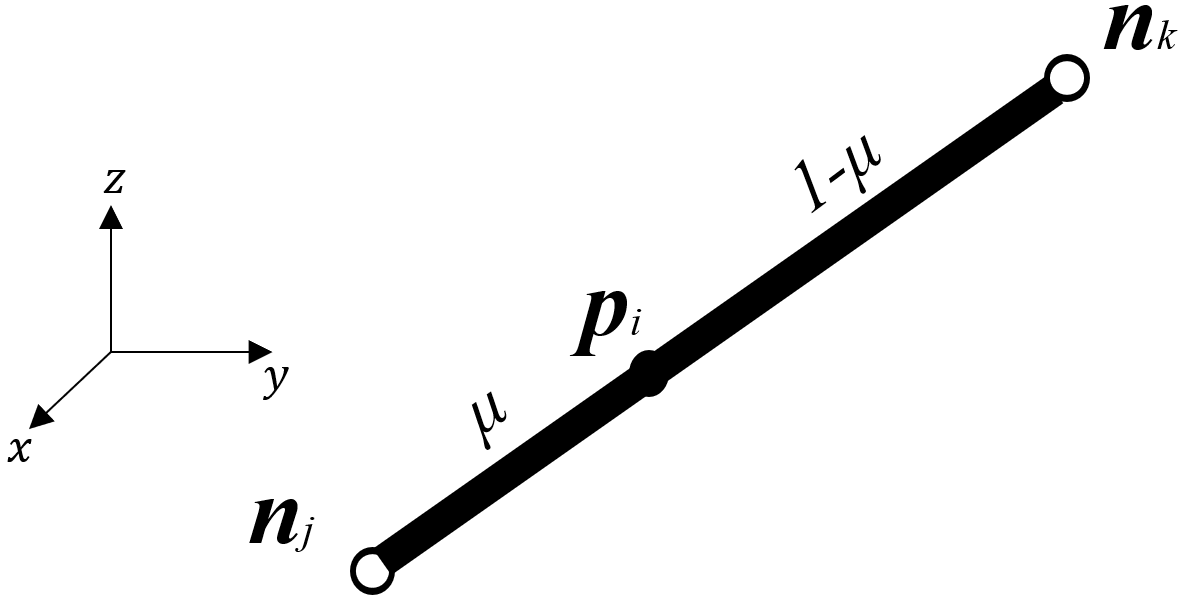
Since both bars and strings are allowed to have elastic or plastic deformation, we do not need to distinguish the connectivity by the types of structural members in this FEM formulation. Thus, we use a matrix $\bm{C}\in\mathbb{R}^{n_{e}\times n_{n}}$ to represent the topology of the whole structure, where $n_{e}$ is the number of all the structural elements, which satisfies $n_{e}=\alpha+\beta$ . The ith row of $\bm{C}$ , denoted as $\bm{C}_{i}=[\bm{C}]_{(i,:)}\in\mathbb{R}^{1\times n_{n}}$ , represents the ith structural element, starting form node j ( $\textit{j}=1,2,\cdots,n_{n}$ ) to node k ( $\textit{k}=1,2,\cdots,n_{n}$ ), shown in Fig.1. The mth ( $\textit{m}=1,2,\cdots,n_{n}$ ) entry of $\bm{C}_{i}$ satisfies:

\displaystyle[\bm{C}]_{im}=\left\{\begin{aligned} -1&,\penalty\ m=j\\ 1&,\penalty\ m=k\\ 0&,\penalty\ m=else\end{aligned}\right..

(4)

For $n_{e}$ number of structural elements, the overall structure connectivity matrix $\bm{C}\in\mathbb{R}^{n_{e}\times n_{n}}$ can be written as:

\displaystyle\bm{C}=\begin{bmatrix}\bm{C}_{1}^{T}&\bm{C}_{2}^{T}&\cdots&\bm{C}_{n_{e}}^{T}\end{bmatrix}^{T}.

(5)

Define the nodal coordinate vector of the ith element $\bm{n}_{i}^{e}\in\mathbb{R}^{6}$ as:

\displaystyle\bm{n}_{i}^{e}=\begin{bmatrix}\bm{n}_{j}\\ \bm{n}_{k}\\ \end{bmatrix}=\begin{bmatrix}x_{j}&y_{j}&z_{j}&x_{k}&y_{k}&z_{k}\end{bmatrix}^{T}.

(6)

One can also abstract $\bm{n}_{i}^{e}$ from the structure nodal coordinate vector $\bm{n}$ :

\displaystyle\bm{n}_{i}^{e}=\bar{\bm{C}}_{i}\otimes\textbf{I}_{3}\bm{n},

(7)

where $\textbf{I}_{3}\in\mathbb{R}^{3\times 3}$ is a identity matrix, $\bar{\bm{C}}_{i}$ is a self-defined transformation matrix, whose pth column satisfies:

\displaystyle[\bar{C}_{i}]_{(:,p)}=\left\{\begin{array}[]{ll}{\begin{bmatrix}1&0\end{bmatrix}^{T}},&p=j\\ {\begin{bmatrix}0&1\end{bmatrix}^{T}},&p=k\\ {\begin{bmatrix}0&0\end{bmatrix}^{T}},&p=else\end{array}\right..

2.4 Geometric properties of the structural elements

Refer to caption — Figure 1: Structure member vector $\bm{h}_{i}$ , determined by node $\bm{n}_{j}$ and node $\bm{n}_{k}$ in the Cartesian coordinates, has a length of $l_{i}=||\bm{h}_{i}||=l_{0i}+\Delta l_{i}$ , where $l_{0i}$ is the rest length and $\Delta l_{i}$ is the displacement.

Let us look at the $i$ th structure element $\bm{h}_{i}$ , its geometry properties is shown in Fig.1, the element vector is given by:

\displaystyle\bm{h}_{i}=\bm{n}_{k}-\bm{n}_{j}=\bm{C}_{i}\otimes\textbf{I}_{3}\bm{n}.

(11)

Stack all the structure elements in a matrix form, one can obtain:

\displaystyle\bm{H}=\begin{bmatrix}\bm{h}_{1}&\bm{h}_{2}&\cdots&\bm{h}_{n_{e}}\end{bmatrix}=\bm{N}\bm{C}^{T}.

(12)

The length of the ith structure element $l_{i}$ satisfies:

\displaystyle l_{i}=\lVert\bm{h}_{i}\rVert=(\bm{n}^{T}(\bm{C}_{i}^{T}\bm{C}_{i})\otimes\textbf{I}_{3}\bm{n})^{\frac{1}{2}}.

(13)

Then, the overall structure element length vector $\bm{l}\in\mathbb{R}^{n_{e}}$ is:

\displaystyle\bm{l}=\begin{bmatrix}l_{1}&l_{2}&\cdots&l_{n_{e}}\end{bmatrix}^{T}.

(14)

The rest length vector $\bm{l}_{0}\in\mathbb{R}^{n_{e}}$ of the whole structure is:

\displaystyle\bm{l}_{0}=\begin{bmatrix}l_{01}&l_{02}&\cdots&l_{0{n_{e}}}\end{bmatrix}^{T},

(15)

where rest length is defined as the length of an structure element with no tension or compression.

2.5 Physical properties of the structural elements

A typical stress-strain curve of an element is given in Fig.2. The stress in the element satisfies:

\sigma=E\epsilon,

(16)

where $E$ is the secant modulus and $\epsilon$ is the strain, and this equation can represent the stress of any material including linear elastic, multi-linear elastic, plastic, etc. The derivative of Eq. (16) is:

\mathrm{d}\sigma=E_{t}\mathrm{d}\epsilon,

(17)

where $E_{t}$ is tangent modulus. For elastic material, the secant modulus is identical to its tangent modulus. We discuss the elastic and plastic properties of materials here because later we will show that the developed dynamics are capable of doing analysis of both kinds of materials.

Suppose material density is $\rho$ , the cross section area, secant modulus, tangent modulus of the ith element are respectively $A_{i}$ , $E_{i}$ $E_{ti}$ , the element mass $m_{i}$ satisfies $m_{i}=\rho A_{i}l_{0i}$ . Denote the cross section area vector, mass vector, secant modulus and tangent modulus vector of the structure as $\bm{A}$ , $\bm{m}$ , $\bm{E}$ and $\bm{E}_{t}$ $\in\mathbb{R}^{n_{e}}$ , one can write:

$\displaystyle\bm{A}$	$\displaystyle=\begin{bmatrix}A_{1}&A_{2}&\cdots&A_{n_{e}}\end{bmatrix}^{T},$	(18)
$\displaystyle\bm{m}$	$\displaystyle=\begin{bmatrix}m_{1}&m_{2}&\cdots&m_{n_{e}}\end{bmatrix}^{T}=\rho\hat{\bm{A}}\bm{l}_{0},$	(19)
$\displaystyle\bm{E}$	$\displaystyle=\begin{bmatrix}E_{1}&E_{2}&\cdots&E_{n_{e}}\end{bmatrix}^{T},$	(20)
$\displaystyle\bm{E}_{t}$	$\displaystyle=\begin{bmatrix}E_{t1}&E_{t2}&\cdots&E_{tn_{e}}\end{bmatrix}^{T},$	(21)

where $\hat{\bm{v}}$ transforms vector $\bm{v}$ into a diagonal matrix, whose diagonal entries are the elements of vector $\bm{v}$ and elsewhere are zeros.

The internal force of the ith element is $t_{i}=A_{i}\sigma_{i}=E_{i}A_{i}(l_{i}-l_{0i})/l_{0i}$ , the internal force vector of the structure $\bm{t}\in\mathbb{R}^{n_{e}}$ can be written as:

\displaystyle\bm{t}=\begin{bmatrix}t_{1}&t_{2}&\cdots&t_{n_{e}}\end{bmatrix}^{T}=\hat{\bm{E}}\hat{\bm{A}}\hat{\bm{l}}_{0}^{-1}(\bm{l}-\bm{l}_{0}).

(22)

Force density of the ith element is given by $x_{i}=t_{i}/l_{i}$ , the force density vector of all the structure elements is:

\displaystyle\bm{x}=\hat{\bm{l}}^{-1}\bm{t}=\hat{\bm{E}}\hat{\bm{A}}(\bm{l}_{0}^{-1}-\bm{l}^{-1}),

(23)

where $\bm{\bm{v}}^{-1}$ represents a vector whose entry is the reciprocal of its corresponding entry in $\bm{v}$ . The force density vector $\bm{x}$ is normally defined in the from of $\bm{x}=\begin{bmatrix}\bm{\lambda}^{T}&\bm{{\gamma}}^{T}\end{bmatrix}^{T}$ with the information of ${\bm{\lambda}}$ and ${\bm{\gamma}}$ are force densities in the bars and strings [5]. We should point out that Eqs. (22) and (23) can be used to compute force vector and force density vector for either elastic or plastic materials by using different secant modulus E of the materials.

3 Nonlinear tensegrity dynamics formulation

3.1 Energy equation formulation

3.1.1 Shape function of the structure element

Since the structure member is axially loaded, the displacement of the material particles are along the bar/string vectors. We assume the displacements of material particles on the structure member are in a uniform manner [1]. Here, we introduce a scalar $\mu$ to help expressing the coordinates of point $\bm{p}_{i}$ on the $i$ th member between node $\bm{n}_{j}$ and node $\bm{n}_{k}$ in the ith structure element, shown in Fig.3. Thus, the location of a point $\bm{p}_{i}$ on the structure member can be computed as a linear function in terms of $\mu$ :

\displaystyle\bm{p_{i}}=\begin{bmatrix}1&\mu\end{bmatrix}\otimes\textbf{I}_{3}\begin{bmatrix}\bm{a}_{0}\\ \bm{a}_{1}\end{bmatrix},

(24)

where $\bm{a}_{0}$ and $\bm{a}_{1}$ $\in\mathbb{R}^{3}$ are unknowns. Substitute the nodal coordinate of $\bm{n}_{j}$ , $\bm{n}_{k}$ with $\mu$ = 0 and 1 into Eq. (24), we have:

\displaystyle\begin{bmatrix}1&0\\ 1&1\end{bmatrix}\otimes\textbf{I}_{3}\begin{bmatrix}\bm{a}_{0}\\ \bm{a}_{1}\end{bmatrix}=\begin{bmatrix}\bm{n}_{j}\\ \bm{n}_{k}\end{bmatrix}.

(25)

Then, the solution of Eq. (25) is:

\displaystyle\begin{bmatrix}\bm{a}_{0}\\ \bm{a}_{1}\end{bmatrix}=\begin{bmatrix}1&0\\ -1&1\end{bmatrix}\otimes\textbf{I}_{3}\begin{bmatrix}\bm{n}_{j}\\ \bm{n}_{k}\end{bmatrix}.

(26)

Substitute Eq. (26) into Eq. (24), we have:

	$\displaystyle\bm{p}_{i}$	$\displaystyle=\begin{bmatrix}1-\mu&\mu\end{bmatrix}\otimes\textbf{I}_{3}\begin{bmatrix}\bm{n}_{j}\\ \bm{n}_{k}\end{bmatrix}=\bm{N}^{e}\bm{n}_{i}^{e},$		(27)
	$\displaystyle\bm{N}^{e}$	$\displaystyle=\begin{bmatrix}1-\mu&\mu\end{bmatrix}\otimes\textbf{I}_{3},$		(28)

where $\bm{N}^{e}\in\mathbb{R}^{3\times 6}$ is usually called the shape function of a structure element.

3.1.2 Kinetic energy

The kinetic energy $T$ for the whole structure equals the sum of kinetic energy of material particles in all the structure elements, which can be written as a function of particle velocity $\dot{\bm{p}}_{i}$ :

\displaystyle T=\sum\limits_{i=1}^{n_{e}}\frac{1}{2}\int\limits_{0}^{1}m_{i}\lVert\dot{\bm{p}}_{i}\rVert^{2}d\mu.

(29)

Substitute Eq. (7) and Eq. (27) into Eq. (29), we have:

$\displaystyle T$	$\displaystyle=\sum\limits_{i=1}^{n_{e}}\frac{1}{2}\int\limits_{0}^{1}m_{i}(\bm{N}^{e}\bar{\bm{C}}_{i}\otimes\textbf{I}_{3}\dot{\bm{n}})^{2}d\mu$	(30)
	$\displaystyle=\sum\limits_{i=1}^{n_{e}}\frac{m_{i}}{12}\dot{\bm{n}}^{T}(\bar{\bm{C}}_{i}^{T}\begin{bmatrix}2&1\\ 1&2\end{bmatrix}\bar{\bm{C}}_{i})\otimes\textbf{I}_{3}\dot{\bm{n}}$	(31)
	$\displaystyle=\sum\limits_{i=1}^{n_{e}}\frac{m_{i}}{12}\dot{\bm{n}}^{T}(\bar{\bm{C}}_{i}^{T}(\begin{bmatrix}1\\ 1\end{bmatrix}[1\penalty\ 1]+\lfloor\begin{bmatrix}1\\ 1\end{bmatrix}[1\penalty\ 1]\rfloor)\bar{\bm{C}}_{i})\otimes\textbf{I}_{3}\dot{\bm{n}}$	(32)
	$\displaystyle=\sum\limits_{i=1}^{n_{e}}\frac{1}{12}\dot{\bm{n}}^{T}(\|\bm{C}\|_{i}^{T}m_{i}\|\bm{C}\|_{i}+\lfloor\|\bm{C}\|_{i}^{T}m_{i}\|\bm{C}\|_{i}\rfloor)\otimes\textbf{I}_{3}\dot{\bm{n}}$	(33)
	$\displaystyle=\frac{1}{12}\dot{\bm{n}}^{T}(\|\bm{C}\|^{T}\hat{m}\|\bm{C}\|+\lfloor\|\bm{C}\|^{T}\hat{m}\|\bm{C}\|\rfloor)\otimes\textbf{I}_{3}\dot{\bm{n}}$	(34)
	$\displaystyle=\frac{1}{2}\dot{\bm{n}}^{T}\bm{M}\dot{\bm{n}},$	(35)

where $|\bm{V}|$ is an operator getting the absolute value of each element for a given matrix, and the operator $\lfloor\bm{V}\rfloor$ sets every off-diagonal element of the square matrix to zero. $\bm{M}\in\mathbb{R}^{3n_{n}\times 3n_{n}}$ is called the mass matrix of the structure:

\displaystyle\bm{M}=\frac{1}{6}(|\bm{C}|^{T}\hat{\bm{m}}|\bm{C}|+\lfloor|\bm{C}|^{T}\hat{\bm{m}}|\bm{C}|\rfloor)\otimes\textbf{I}_{3}.

(36)

Since the matrix $\bm{M}$ is symmetric, we can have the following equation:

\displaystyle\frac{\mathrm{d}}{\mathrm{d}t}\frac{\partial T}{\partial\dot{\bm{n}}}=\bm{M}\ddot{\bm{n}}.

(37)

Note that we use denominator layout notation in matrix calculus, which means the derivative of a scalar by a column vector is still a column vector.

3.1.3 Strain potential energy

We consider elastic and plastic deformation of structure members, to unify the two cases, the strain potential energy $V_{e}$ of the whole structure caused by elements’ internal force can be written into an integral form:

$\displaystyle V_{e}$	$\displaystyle=\sum\limits_{i}^{n_{e}}V_{ei}$	(38)
	$\displaystyle=\sum\limits_{i}^{n_{e}}\int_{l_{0i}}^{l_{i}}t_{i}\mathrm{d}u$	(39)
	$\displaystyle=\sum\limits_{i}^{n_{e}}\int_{l_{0i}}^{l_{i}}\frac{E_{i}A_{i}(u-l_{0i})}{l_{0i}}\mathrm{d}u,$	(40)

where $\mathrm{d}u$ is the differential of the structure member length. The derivative of strain potential energy $V_{e}$ with respect to nodal coordinate vector $\bm{n}$ is:

$\displaystyle\frac{\partial V_{e}}{\partial\bm{n}}$	$\displaystyle=\sum\limits_{i}^{n_{e}}\frac{\partial V_{ei}}{\partial l_{i}}\frac{\partial l_{i}}{\partial\bm{n}}$	(41)
	$\displaystyle=\sum\limits_{i}^{n_{e}}\frac{E_{i}A_{i}(l_{i}-l_{0i})}{l_{0i}}\frac{\partial l_{i}}{\partial\bm{n}}$	(42)
	$\displaystyle=\sum\limits_{i}^{n_{e}}t_{i}\frac{\partial l_{i}}{\partial\bm{n}}.$	(43)

The derivative of element’s length $l_{i}$ with respect to nodal coordinate vector $\bm{n}$ can be obtained from Eq. (13):

\displaystyle\frac{\partial l_{i}}{\partial\bm{n}}=\frac{(\bm{C}_{i}^{T}\bm{C}_{i})\otimes\textbf{I}_{3}\bm{n}}{l_{i}}.

(44)

Substitute Eq. (44) into Eq. (43), and use the definition of force density $x_{i}=f_{i}/l_{i}$ in the ith structure element, we have:

$\displaystyle\frac{\partial V_{e}}{\partial\bm{n}}$	$\displaystyle=\sum\limits_{i}^{n_{e}}x_{i}(\bm{C}_{i}^{T}\bm{C}_{i})\otimes\textbf{I}_{3}\bm{n}$	(45)
	$\displaystyle=(\bm{C}^{T}\hat{\bm{x}}\bm{C})\otimes\textbf{I}_{3}\bm{n}$	(46)
	$\displaystyle=\bm{Kn},$	(47)

where $\bm{K}\in\mathbb{R}^{3n_{n}\times 3n_{n}}$ is the stiffness matrix of the tensegrity structure:

\displaystyle\bm{K}=(\bm{C}^{T}\hat{\bm{x}}\bm{C})\otimes\textbf{I}_{3}.

(48)

3.1.4 Gravitational potential energy

For many cases that the tensegrity structures are in the presence of gravity field. Suppose the gravity force is exerted towards the negative direction of the Z-axis, the acceleration of gravity is $g$ , for example, on earth $g=9.8m/s^{2}$ . The gravitational potential energy $V_{g}$ can be written as:

$\displaystyle V_{g}$	$\displaystyle=\sum\limits_{i}^{n_{e}}\frac{m_{i}g}{2}(z^{i}_{j}+z^{i}_{k})$	(49)
	$\displaystyle=\sum\limits_{i}^{n_{e}}\frac{m_{i}g}{2}\|\bm{C}_{i}\|\otimes\begin{bmatrix}0&0&1\end{bmatrix}\bm{n}$	(50)
	$\displaystyle=\frac{g}{2}\bm{m}^{T}\|\bm{C}\|\otimes\begin{bmatrix}0&0&1\end{bmatrix}\bm{n},$	(51)

where $z^{i}_{j}$ and $z^{i}_{k}$ are Z-coordinates of node $\bm{n}_{j}$ and node $\bm{n}_{k}$ of the ith structure element. $(z^{i}_{j}+z^{i}_{k})/2$ is the Z-coordinate of mass center of the ith element. Then, the partial derivative of $V_{g}$ with respect to $\bm{n}$ is:

\displaystyle\frac{\partial V_{g}}{\partial\bm{n}}=\frac{g}{2}(|\bm{C}|^{T}\bm{m})\otimes\begin{bmatrix}0&0&1\end{bmatrix}^{T}=\bm{g},

(52)

where $\bm{g}\in\mathbb{R}^{3n_{n}}$ is the gravitational force vector in all nodes. For structure analysis without gravity, one can just set $\bm{g}=\bm{0}$ .

3.2 Tensegrity dynamics formulation based on Lagrangian method

Theorem 3.1.

The finite element formulation for nonlinear tensegrity dynamics in the presence of gravity is given by:

\bm{M}\ddot{\bm{n}}+\bm{D}\dot{\bm{n}}+\bm{K}\bm{n}=\bm{f}_{ex}-\bm{g},

(53)

where $\bm{M}$ , $\bm{D}$ , and $\bm{K}$ are mass, damping, and stiffness matrices given in Eqs. (36), (59), and (48), $f_{ex}$ is external forces on the structure nodes, and $\bm{g}$ is gravity vector show in Eq. (52).

Proof.

The dynamics of tensegrity structures can be derived by Lagrangian method. The Lagrangian equation is:

\displaystyle\frac{\mathrm{d}}{\mathrm{d}t}\frac{\partial L}{\partial\dot{\bm{q}}}-\frac{\partial L}{\partial\bm{q}}=\bm{f}_{np},

(54)

where $L=T-V$ is the Lagrangian function, and $T$ and $V$ are the kinetic energy and potential energy of the system, $\bm{f}_{np}$ is the non-potential force vector on the nodes of the tensegrity structures, and $\bm{q}$ is the generalized coordinate of the system, which is nodal coordinate vector $\bm{n}$ in our derivation. The potential energy of the whole structure is the sum of strain energy $V_{e}$ and gravitational potential energy $V_{g}$ :

\displaystyle V=V_{e}+V_{g}.

(55)

Then, the Lagrangian’s function can be written as:

\displaystyle L=T-(V_{e}+V_{g}).

(56)

Substitute Eqs. (37), (47), (52), (56) into Eq. (54), we have the dynamic equation of the tensegrity structure:

\displaystyle\bm{M}\ddot{\bm{n}}+\bm{Kn}=\bm{f}_{np}-\bm{g},

(57)

where $\bm{M}\in\mathbb{R}^{3n_{n}\times 3n_{n}}$ , $\bm{K}\in\mathbb{R}^{3n_{n}\times 3n_{n}}$ , $\bm{g}\in\mathbb{R}^{3n_{n}}$ are mass matrix, stiffness matrix and gravitational force vector, given in Eq. (36), Eq. (48), and Eq. (52). The non-potential force $\bm{f}_{np}$ is the sum of damping force $\bm{f}_{d}$ and external force $\bm{f}_{ex}$ :

\displaystyle\bm{f}_{np}=\bm{f}_{d}+\bm{f}_{ex}.

(58)

The damping force is assumed to be linear in terms of $\dot{n}$ as:

\displaystyle\bm{f}_{d}=-\bm{D}\dot{\bm{n}},

(59)

where $\bm{D}\in\mathbb{R}^{3n_{n}\times 3n_{n}}$ is the damping matrix of the structure. Substitute Eq. (58) and Eq. (59) into Eq. (57), we can obtain a standard form of the dynamics equation as in Eq. (53).

∎

3.3 Tensegrity dynamics with constraints

By constraints, we mean, for many cases, the position, velocity, or acceleration of some nodes in the structure are fixed/given. Adding these constraints to the dynamics will restrict the motion in certain dimensions, thus the dynamics Eq. (53) can be reduced into a smaller space. Thus, to compute the reduced-order dynamics, free nodes and fix nodes must be separated.

Let us define vector $\bm{a}=\begin{bmatrix}a_{1}&a_{2}&\cdots&a_{n_{a}}\end{bmatrix}^{T}\in\mathbb{R}^{n_{a}}$ and vector $\bm{b}=\begin{bmatrix}b_{1}&b_{2}&\cdots&b_{n_{b}}\end{bmatrix}^{T}\in\mathbb{R}^{n_{b}}$ , in which the element values of $\bm{a}$ and $\bm{b}$ are the indices of free and constrained entries in the nodal coordinate vector n. $n_{a}$ and $n_{b}$ is the number of free and constrained nodal coordinates, and they satisfy $n_{a}+n_{b}=3n_{n}$ . We use $\bm{n}_{a}$ and $\bm{n}_{b}$ to represent the free and constrained nodal coordinate vector. $\bm{E}_{a}\in\mathbb{R}^{3n_{n}\times n_{a}}$ and $\bm{E}_{b}\in\mathbb{R}^{3n_{n}\times n_{b}}$ are the matrix to abstract $\bm{n}_{a}$ and $\bm{n}_{b}$ from $\bm{n}$ :

\displaystyle\bm{E}_{a}(:,i)=\textbf{I}_{3n}\left(:,a_{i}\right),\penalty\ \bm{E}_{b}(:,i)=\textbf{I}_{3n}\left(:,b_{i}\right).

(60)

The relation between $\bm{n}_{a}$ , $\bm{n}_{b}$ , and $\bm{n}$ is:

\displaystyle\bm{n}_{a}=\bm{E}_{a}^{T}\bm{n},\penalty\ \bm{n}_{b}=\bm{E}_{b}^{T}\bm{n}.

(61)

Note that $\begin{bmatrix}\bm{E}_{a}&\bm{E}_{b}\end{bmatrix}$ is an orthonormal matrix, so given $\bm{n}_{a}$ and $\bm{n}_{b}$ , the nodal coordinate vector $\bm{n}$ can be obtained by:

\displaystyle\bm{n}=\begin{bmatrix}\bm{E}_{a}^{T}\\ \bm{E}_{b}^{T}\end{bmatrix}^{-1}\begin{bmatrix}\bm{n}_{a}\\ \bm{n}_{b}\end{bmatrix}=\begin{bmatrix}\bm{E}_{a}&\bm{E}_{b}\end{bmatrix}\begin{bmatrix}\bm{n}_{a}\\ \bm{n}_{b}\end{bmatrix}.

(62)

Theorem 3.2.

The finite element formulation for nonlinear tensegrity dynamics in the presence of constraints and gravity is given by:

	$\displaystyle\bm{M}_{aa}\ddot{\bm{n}}_{a}+\bm{D}_{aa}\dot{\bm{n}}_{a}+\bm{K}_{aa}\bm{n}_{a}=$	$\displaystyle\bm{E}_{a}^{T}\bm{f}_{ex}-\bm{M}_{ab}\ddot{\bm{n}}_{b}-\bm{D}_{ab}\dot{\bm{n}}_{b}$
		$\displaystyle-\bm{K}_{ab}\bm{n}_{b}-\bm{E}_{a}^{T}\bm{g},$		(63)

where $\bm{M}_{aa}$ and $\bm{M}_{ab}$ are mass matrices. $\bm{D}_{aa}$ and $\bm{D}_{ab}$ are damping matrices. $\bm{K}_{aa}$ and $\bm{K}_{ab}$ are stiffness matrices. $\bm{f}_{ex}$ is external forces on the structure nodes, and $\bm{g}$ is gravity vector, which satisfy:

$\displaystyle\bm{M}_{aa}$	$\displaystyle=\bm{E}_{a}^{T}\bm{M}\bm{E}_{a},\penalty\ \bm{M}_{ab}=\bm{E}_{a}^{T}\bm{M}\bm{E}_{b},$	(64)
$\displaystyle\bm{D}_{aa}$	$\displaystyle=\bm{E}_{a}^{T}\bm{D}\bm{E}_{a},\penalty\ \bm{D}_{ab}=\bm{E}_{a}^{T}\bm{D}\bm{E}_{b},$	(65)
$\displaystyle\bm{K}_{aa}$	$\displaystyle=\bm{E}_{a}^{T}\bm{K}\bm{E}_{a},\penalty\ \bm{K}_{ab}=\bm{E}_{a}^{T}\bm{K}\bm{E}_{b},$	(66)

and $\bm{M}$ , $\bm{D}$ , $\bm{K}$ , and $\bm{g}$ are given in Eqs. (36), (59), (48), and (52).

Proof.

If the tensegrity structure has boundary constraints, the degree of freedom reduces to $n_{a}$ , thus the free nodal coordinate vector $\bm{n}_{a}$ is the generalized coordinate. Then, the Lagrange’s equation is:

\displaystyle\frac{\mathrm{d}}{\mathrm{dt}}\left(\frac{\partial L}{\partial\dot{\bm{n}}_{a}}\right)-\frac{\partial L}{\partial\bm{n}_{a}}=\bm{f}_{npa},

(67)

where $\bm{f}_{npa}$ is the non-potential force exerted on free nodal coordinate, and its relation with $\bm{f}_{np}$ is:

\displaystyle\bm{f}_{npa}=\bm{E}_{a}^{T}\bm{f}_{np}.

(68)

The relation of left side of Eq. (67) and Eq. (54) is:

	$\displaystyle\frac{\mathrm{d}}{\mathrm{dt}}\left(\frac{\partial L}{\partial\dot{\bm{n}}_{a}}\right)$	$\displaystyle-\frac{\partial L}{\partial\bm{n}_{a}}=\frac{\partial\bm{n}}{\partial\bm{n}_{a}}\left[\frac{\mathrm{d}}{\mathrm{dt}}\left(\frac{\partial L}{\partial\dot{\bm{n}}}\right)-\frac{\partial L}{\partial\bm{n}}\right]$		(69)
		$\displaystyle=\bm{E}_{a}^{T}\left[\frac{\mathrm{d}}{\mathrm{dt}}\left(\frac{\partial L}{\partial\dot{\bm{n}}}\right)-\frac{\partial L}{\partial\bm{n}}\right].$		(70)

Substitute Eqs. (68), (70) into Eq. (67), we have the dynamics of tensegrity for the free nodal coordinates:

\displaystyle\bm{E}_{a}^{T}(\bm{M}\ddot{\bm{n}}+\bm{D}\dot{\bm{n}}+\bm{K}\bm{n})=\bm{E}_{a}^{T}\left(\bm{f}_{ex}-\bm{g}\right).

(71)

From the above equation, we can see that the dynamic equation Eq. (71) with constraints is just the $\bm{a}$ rows of Eq. (53). Substitute Eq. (62) into Eq. (71) and arrange terms related to $\bm{n}_{a}$ in left side, we obtain Eq. (63). We can also have the following form in term of $\ddot{\bm{n}}_{a}$ for programming convenience:

\displaystyle\ddot{\bm{n}}_{a}=\bm{M}_{aa}^{-1}\bm{E}_{a}^{T}\left(\bm{f}_{ex}-\bm{g}-\bm{M}\bm{E}_{b}\ddot{\bm{n}}_{b}-\bm{D}\dot{\bm{n}}-\bm{K}\bm{n}\right).

(72)

∎

3.4 Static equilibrium equation

The static equilibrium equation can be easily obtained from the derived dynamics equation. Here, we give the equilibrium equation in three standard forms and the compatibility equation. The equations developed in this section are useful for the derivation of the linearized dynamics in the next section.

Theorem 3.3.

The three following tensegrity static equilibrium equations are equivalent:

1). Tensegrity statics in terms of nodal coordinate vector $\bm{n}$ :

\displaystyle\bm{K}\bm{n}=\bm{f}_{ex}-\bm{g},\penalty\ \bm{K}=(\bm{C}^{T}\hat{\bm{x}}\bm{C})\otimes\textbf{I}_{3}.

(73)

2). Tensegrity statics in terms of force density vector $\bm{x}$ :

\displaystyle\bm{A}_{1}\bm{x}=\bm{f}_{ex}-\bm{g},\penalty\ \bm{A}_{1}=\left(\bm{C}^{T}\otimes\textbf{I}_{3}\right)\bm{b.d.}(\bm{H}).

(74)

3). Tensegrity statics in terms of force vector $\bm{t}$ :

\displaystyle\bm{A}_{2}\bm{t}=\bm{f}_{ex}-\bm{g},\penalty\ \bm{A}_{2}=\left(\bm{C}^{T}\otimes\textbf{I}_{3}\right)\bm{b.d.}(\bm{H})\hat{\bm{l}}^{-1}.

(75)

Proof.

Let the acceleration part $\ddot{\bm{n}}$ and velocity part $\dot{\bm{n}}$ in Eq. (53) be zeros, the dynamics equation will be reduced into a static equilibrium equation in terms of nodal coordinate vector $\bm{n}$ :

\displaystyle\bm{K}\bm{n}=\bm{f}_{ex}-\bm{g}.

(76)

This proofs the first statement of Theorem 3.3.

Since $\bm{K}$ , given in Eq. (48), is a function of $\bm{n}$ , the product $\bm{Kn}$ is nonlinear in $\bm{n}$ . Eq. (76) is a nonlinear equilibrium equation. However, the term $\bm{Kn}$ can be also written linearly in terms of force density vector $\bm{x}$ :

$\displaystyle\bm{K}\bm{n}$	$\displaystyle=\left(\bm{C}^{T}\otimes\textbf{I}_{3}\right)\left(\widehat{\bm{x}}\otimes\textbf{I}_{3}\right)\left(\bm{C}\otimes\textbf{I}_{3}\right)\bm{n}$	(77)
	$\displaystyle=\left(\bm{C}^{T}\otimes\textbf{I}_{3}\right)\begin{array}[]{c}\mathchoice{\raisebox{-3.34055pt}{\resizebox{53617400}{141084}{\hbox{\raisebox{10.00012pt}{$\displaystyle\mathchoice{\raisebox{-853.45891pt}{\resizebox{468892385}{36044800}{\hbox{\raisebox{10.00012pt}{$\displaystyle\mathchoice{\raisebox{0.0pt}{\resizebox{0}{0}{\hbox{\raisebox{10.00012pt}{$\displaystyle\kern-0.5pt\bigwedge\kern-0.5pt$}}}}}{\raisebox{0.0pt}{\resizebox{0}{0}{\hbox{\raisebox{10.00012pt}{$\textstyle\kern-0.5pt\bigwedge\kern-0.5pt$}}}}}{\raisebox{0.0pt}{\resizebox{0}{0}{\hbox{\raisebox{1.4pt}{$\scriptstyle\kern-0.5pt\bigwedge\kern-0.5pt$}}}}}{\raisebox{0.0pt}{\resizebox{0}{0}{\hbox{\raisebox{1.0pt}{$\scriptscriptstyle\kern-0.5pt\bigwedge\kern-0.5pt$}}}}}$}}}}}{\raisebox{-853.45891pt}{\resizebox{468892385}{36044800}{\hbox{\raisebox{10.00012pt}{$\textstyle\mathchoice{\raisebox{0.0pt}{\resizebox{0}{0}{\hbox{\raisebox{10.00012pt}{$\displaystyle\kern-0.5pt\bigwedge\kern-0.5pt$}}}}}{\raisebox{0.0pt}{\resizebox{0}{0}{\hbox{\raisebox{10.00012pt}{$\textstyle\kern-0.5pt\bigwedge\kern-0.5pt$}}}}}{\raisebox{0.0pt}{\resizebox{0}{0}{\hbox{\raisebox{1.4pt}{$\scriptstyle\kern-0.5pt\bigwedge\kern-0.5pt$}}}}}{\raisebox{0.0pt}{\resizebox{0}{0}{\hbox{\raisebox{1.0pt}{$\scriptscriptstyle\kern-0.5pt\bigwedge\kern-0.5pt$}}}}}$}}}}}{\raisebox{-157.14236pt}{\resizebox{468892385}{36044800}{\hbox{\raisebox{1.4pt}{$\scriptstyle\mathchoice{\raisebox{0.0pt}{\resizebox{0}{0}{\hbox{\raisebox{1.4pt}{$\displaystyle\kern-0.5pt\bigwedge\kern-0.5pt$}}}}}{\raisebox{0.0pt}{\resizebox{0}{0}{\hbox{\raisebox{1.4pt}{$\textstyle\kern-0.5pt\bigwedge\kern-0.5pt$}}}}}{\raisebox{0.0pt}{\resizebox{0}{0}{\hbox{\raisebox{0.98pt}{$\scriptstyle\kern-0.5pt\bigwedge\kern-0.5pt$}}}}}{\raisebox{0.0pt}{\resizebox{0}{0}{\hbox{\raisebox{0.7pt}{$\scriptscriptstyle\kern-0.5pt\bigwedge\kern-0.5pt$}}}}}$}}}}}{\raisebox{-157.14285pt}{\resizebox{468892385}{36044800}{\hbox{\raisebox{1.0pt}{$\scriptscriptstyle\mathchoice{\raisebox{0.0pt}{\resizebox{0}{0}{\hbox{\raisebox{1.0pt}{$\displaystyle\kern-0.5pt\bigwedge\kern-0.5pt$}}}}}{\raisebox{0.0pt}{\resizebox{0}{0}{\hbox{\raisebox{1.0pt}{$\textstyle\kern-0.5pt\bigwedge\kern-0.5pt$}}}}}{\raisebox{0.0pt}{\resizebox{0}{0}{\hbox{\raisebox{0.7pt}{$\scriptstyle\kern-0.5pt\bigwedge\kern-0.5pt$}}}}}{\raisebox{0.0pt}{\resizebox{0}{0}{\hbox{\raisebox{0.5pt}{$\scriptscriptstyle\kern-0.5pt\bigwedge\kern-0.5pt$}}}}}$}}}}}$}}}}}{\raisebox{-3.34055pt}{\resizebox{53617400}{141084}{\hbox{\raisebox{10.00012pt}{$\textstyle\mathchoice{\raisebox{-853.45891pt}{\resizebox{468892385}{36044800}{\hbox{\raisebox{10.00012pt}{$\displaystyle\mathchoice{\raisebox{0.0pt}{\resizebox{0}{0}{\hbox{\raisebox{10.00012pt}{$\displaystyle\kern-0.5pt\bigwedge\kern-0.5pt$}}}}}{\raisebox{0.0pt}{\resizebox{0}{0}{\hbox{\raisebox{10.00012pt}{$\textstyle\kern-0.5pt\bigwedge\kern-0.5pt$}}}}}{\raisebox{0.0pt}{\resizebox{0}{0}{\hbox{\raisebox{1.4pt}{$\scriptstyle\kern-0.5pt\bigwedge\kern-0.5pt$}}}}}{\raisebox{0.0pt}{\resizebox{0}{0}{\hbox{\raisebox{1.0pt}{$\scriptscriptstyle\kern-0.5pt\bigwedge\kern-0.5pt$}}}}}$}}}}}{\raisebox{-853.45891pt}{\resizebox{468892385}{36044800}{\hbox{\raisebox{10.00012pt}{$\textstyle\mathchoice{\raisebox{0.0pt}{\resizebox{0}{0}{\hbox{\raisebox{10.00012pt}{$\displaystyle\kern-0.5pt\bigwedge\kern-0.5pt$}}}}}{\raisebox{0.0pt}{\resizebox{0}{0}{\hbox{\raisebox{10.00012pt}{$\textstyle\kern-0.5pt\bigwedge\kern-0.5pt$}}}}}{\raisebox{0.0pt}{\resizebox{0}{0}{\hbox{\raisebox{1.4pt}{$\scriptstyle\kern-0.5pt\bigwedge\kern-0.5pt$}}}}}{\raisebox{0.0pt}{\resizebox{0}{0}{\hbox{\raisebox{1.0pt}{$\scriptscriptstyle\kern-0.5pt\bigwedge\kern-0.5pt$}}}}}$}}}}}{\raisebox{-157.14236pt}{\resizebox{468892385}{36044800}{\hbox{\raisebox{1.4pt}{$\scriptstyle\mathchoice{\raisebox{0.0pt}{\resizebox{0}{0}{\hbox{\raisebox{1.4pt}{$\displaystyle\kern-0.5pt\bigwedge\kern-0.5pt$}}}}}{\raisebox{0.0pt}{\resizebox{0}{0}{\hbox{\raisebox{1.4pt}{$\textstyle\kern-0.5pt\bigwedge\kern-0.5pt$}}}}}{\raisebox{0.0pt}{\resizebox{0}{0}{\hbox{\raisebox{0.98pt}{$\scriptstyle\kern-0.5pt\bigwedge\kern-0.5pt$}}}}}{\raisebox{0.0pt}{\resizebox{0}{0}{\hbox{\raisebox{0.7pt}{$\scriptscriptstyle\kern-0.5pt\bigwedge\kern-0.5pt$}}}}}$}}}}}{\raisebox{-157.14285pt}{\resizebox{468892385}{36044800}{\hbox{\raisebox{1.0pt}{$\scriptscriptstyle\mathchoice{\raisebox{0.0pt}{\resizebox{0}{0}{\hbox{\raisebox{1.0pt}{$\displaystyle\kern-0.5pt\bigwedge\kern-0.5pt$}}}}}{\raisebox{0.0pt}{\resizebox{0}{0}{\hbox{\raisebox{1.0pt}{$\textstyle\kern-0.5pt\bigwedge\kern-0.5pt$}}}}}{\raisebox{0.0pt}{\resizebox{0}{0}{\hbox{\raisebox{0.7pt}{$\scriptstyle\kern-0.5pt\bigwedge\kern-0.5pt$}}}}}{\raisebox{0.0pt}{\resizebox{0}{0}{\hbox{\raisebox{0.5pt}{$\scriptscriptstyle\kern-0.5pt\bigwedge\kern-0.5pt$}}}}}$}}}}}$}}}}}{\raisebox{-0.61507pt}{\resizebox{39915495}{141084}{\hbox{\raisebox{1.4pt}{$\scriptstyle\mathchoice{\raisebox{-157.14236pt}{\resizebox{468892385}{36044800}{\hbox{\raisebox{1.4pt}{$\displaystyle\mathchoice{\raisebox{0.0pt}{\resizebox{0}{0}{\hbox{\raisebox{1.4pt}{$\displaystyle\kern-0.5pt\bigwedge\kern-0.5pt$}}}}}{\raisebox{0.0pt}{\resizebox{0}{0}{\hbox{\raisebox{1.4pt}{$\textstyle\kern-0.5pt\bigwedge\kern-0.5pt$}}}}}{\raisebox{0.0pt}{\resizebox{0}{0}{\hbox{\raisebox{0.98pt}{$\scriptstyle\kern-0.5pt\bigwedge\kern-0.5pt$}}}}}{\raisebox{0.0pt}{\resizebox{0}{0}{\hbox{\raisebox{0.7pt}{$\scriptscriptstyle\kern-0.5pt\bigwedge\kern-0.5pt$}}}}}$}}}}}{\raisebox{-157.14236pt}{\resizebox{468892385}{36044800}{\hbox{\raisebox{1.4pt}{$\textstyle\mathchoice{\raisebox{0.0pt}{\resizebox{0}{0}{\hbox{\raisebox{1.4pt}{$\displaystyle\kern-0.5pt\bigwedge\kern-0.5pt$}}}}}{\raisebox{0.0pt}{\resizebox{0}{0}{\hbox{\raisebox{1.4pt}{$\textstyle\kern-0.5pt\bigwedge\kern-0.5pt$}}}}}{\raisebox{0.0pt}{\resizebox{0}{0}{\hbox{\raisebox{0.98pt}{$\scriptstyle\kern-0.5pt\bigwedge\kern-0.5pt$}}}}}{\raisebox{0.0pt}{\resizebox{0}{0}{\hbox{\raisebox{0.7pt}{$\scriptscriptstyle\kern-0.5pt\bigwedge\kern-0.5pt$}}}}}$}}}}}{\raisebox{-157.1425pt}{\resizebox{468892385}{36044800}{\hbox{\raisebox{0.98pt}{$\scriptstyle\mathchoice{\raisebox{0.0pt}{\resizebox{0}{0}{\hbox{\raisebox{0.98pt}{$\displaystyle\kern-0.5pt\bigwedge\kern-0.5pt$}}}}}{\raisebox{0.0pt}{\resizebox{0}{0}{\hbox{\raisebox{0.98pt}{$\textstyle\kern-0.5pt\bigwedge\kern-0.5pt$}}}}}{\raisebox{0.0pt}{\resizebox{0}{0}{\hbox{\raisebox{0.68599pt}{$\scriptstyle\kern-0.5pt\bigwedge\kern-0.5pt$}}}}}{\raisebox{0.0pt}{\resizebox{0}{0}{\hbox{\raisebox{0.48999pt}{$\scriptscriptstyle\kern-0.5pt\bigwedge\kern-0.5pt$}}}}}$}}}}}{\raisebox{-157.14236pt}{\resizebox{468892385}{36044800}{\hbox{\raisebox{0.7pt}{$\scriptscriptstyle\mathchoice{\raisebox{0.0pt}{\resizebox{0}{0}{\hbox{\raisebox{0.7pt}{$\displaystyle\kern-0.5pt\bigwedge\kern-0.5pt$}}}}}{\raisebox{0.0pt}{\resizebox{0}{0}{\hbox{\raisebox{0.7pt}{$\textstyle\kern-0.5pt\bigwedge\kern-0.5pt$}}}}}{\raisebox{0.0pt}{\resizebox{0}{0}{\hbox{\raisebox{0.48999pt}{$\scriptstyle\kern-0.5pt\bigwedge\kern-0.5pt$}}}}}{\raisebox{0.0pt}{\resizebox{0}{0}{\hbox{\raisebox{0.34999pt}{$\scriptscriptstyle\kern-0.5pt\bigwedge\kern-0.5pt$}}}}}$}}}}}$}}}}}{\raisebox{-0.61507pt}{\resizebox{32849234}{141084}{\hbox{\raisebox{1.0pt}{$\scriptscriptstyle\mathchoice{\raisebox{-157.14285pt}{\resizebox{468892385}{36044800}{\hbox{\raisebox{1.0pt}{$\displaystyle\mathchoice{\raisebox{0.0pt}{\resizebox{0}{0}{\hbox{\raisebox{1.0pt}{$\displaystyle\kern-0.5pt\bigwedge\kern-0.5pt$}}}}}{\raisebox{0.0pt}{\resizebox{0}{0}{\hbox{\raisebox{1.0pt}{$\textstyle\kern-0.5pt\bigwedge\kern-0.5pt$}}}}}{\raisebox{0.0pt}{\resizebox{0}{0}{\hbox{\raisebox{0.7pt}{$\scriptstyle\kern-0.5pt\bigwedge\kern-0.5pt$}}}}}{\raisebox{0.0pt}{\resizebox{0}{0}{\hbox{\raisebox{0.5pt}{$\scriptscriptstyle\kern-0.5pt\bigwedge\kern-0.5pt$}}}}}$}}}}}{\raisebox{-157.14285pt}{\resizebox{468892385}{36044800}{\hbox{\raisebox{1.0pt}{$\textstyle\mathchoice{\raisebox{0.0pt}{\resizebox{0}{0}{\hbox{\raisebox{1.0pt}{$\displaystyle\kern-0.5pt\bigwedge\kern-0.5pt$}}}}}{\raisebox{0.0pt}{\resizebox{0}{0}{\hbox{\raisebox{1.0pt}{$\textstyle\kern-0.5pt\bigwedge\kern-0.5pt$}}}}}{\raisebox{0.0pt}{\resizebox{0}{0}{\hbox{\raisebox{0.7pt}{$\scriptstyle\kern-0.5pt\bigwedge\kern-0.5pt$}}}}}{\raisebox{0.0pt}{\resizebox{0}{0}{\hbox{\raisebox{0.5pt}{$\scriptscriptstyle\kern-0.5pt\bigwedge\kern-0.5pt$}}}}}$}}}}}{\raisebox{-157.14236pt}{\resizebox{468892385}{36044800}{\hbox{\raisebox{0.7pt}{$\scriptstyle\mathchoice{\raisebox{0.0pt}{\resizebox{0}{0}{\hbox{\raisebox{0.7pt}{$\displaystyle\kern-0.5pt\bigwedge\kern-0.5pt$}}}}}{\raisebox{0.0pt}{\resizebox{0}{0}{\hbox{\raisebox{0.7pt}{$\textstyle\kern-0.5pt\bigwedge\kern-0.5pt$}}}}}{\raisebox{0.0pt}{\resizebox{0}{0}{\hbox{\raisebox{0.48999pt}{$\scriptstyle\kern-0.5pt\bigwedge\kern-0.5pt$}}}}}{\raisebox{0.0pt}{\resizebox{0}{0}{\hbox{\raisebox{0.34999pt}{$\scriptscriptstyle\kern-0.5pt\bigwedge\kern-0.5pt$}}}}}$}}}}}{\raisebox{-157.14285pt}{\resizebox{468892385}{36044800}{\hbox{\raisebox{0.5pt}{$\scriptscriptstyle\mathchoice{\raisebox{0.0pt}{\resizebox{0}{0}{\hbox{\raisebox{0.5pt}{$\displaystyle\kern-0.5pt\bigwedge\kern-0.5pt$}}}}}{\raisebox{0.0pt}{\resizebox{0}{0}{\hbox{\raisebox{0.5pt}{$\textstyle\kern-0.5pt\bigwedge\kern-0.5pt$}}}}}{\raisebox{0.0pt}{\resizebox{0}{0}{\hbox{\raisebox{0.34999pt}{$\scriptstyle\kern-0.5pt\bigwedge\kern-0.5pt$}}}}}{\raisebox{0.0pt}{\resizebox{0}{0}{\hbox{\raisebox{0.25pt}{$\scriptscriptstyle\kern-0.5pt\bigwedge\kern-0.5pt$}}}}}$}}}}}$}}}}}\\ \left(\textbf{I}_{n_{e}}\otimes\textbf{I}_{3,1}\bm{x}\right)\\ \rule{-4.30554pt}{0.0pt}\end{array}\left(\bm{C}\otimes\textbf{I}_{3}\right)\bm{n}$
	$\displaystyle=\left(\bm{C}^{T}\otimes\textbf{I}_{3}\right)\begin{array}[]{c}\mathchoice{\raisebox{-3.34055pt}{\resizebox{53617400}{141084}{\hbox{\raisebox{10.00012pt}{$\displaystyle\mathchoice{\raisebox{-853.45891pt}{\resizebox{468892385}{36044800}{\hbox{\raisebox{10.00012pt}{$\displaystyle\mathchoice{\raisebox{0.0pt}{\resizebox{0}{0}{\hbox{\raisebox{10.00012pt}{$\displaystyle\kern-0.5pt\bigwedge\kern-0.5pt$}}}}}{\raisebox{0.0pt}{\resizebox{0}{0}{\hbox{\raisebox{10.00012pt}{$\textstyle\kern-0.5pt\bigwedge\kern-0.5pt$}}}}}{\raisebox{0.0pt}{\resizebox{0}{0}{\hbox{\raisebox{1.4pt}{$\scriptstyle\kern-0.5pt\bigwedge\kern-0.5pt$}}}}}{\raisebox{0.0pt}{\resizebox{0}{0}{\hbox{\raisebox{1.0pt}{$\scriptscriptstyle\kern-0.5pt\bigwedge\kern-0.5pt$}}}}}$}}}}}{\raisebox{-853.45891pt}{\resizebox{468892385}{36044800}{\hbox{\raisebox{10.00012pt}{$\textstyle\mathchoice{\raisebox{0.0pt}{\resizebox{0}{0}{\hbox{\raisebox{10.00012pt}{$\displaystyle\kern-0.5pt\bigwedge\kern-0.5pt$}}}}}{\raisebox{0.0pt}{\resizebox{0}{0}{\hbox{\raisebox{10.00012pt}{$\textstyle\kern-0.5pt\bigwedge\kern-0.5pt$}}}}}{\raisebox{0.0pt}{\resizebox{0}{0}{\hbox{\raisebox{1.4pt}{$\scriptstyle\kern-0.5pt\bigwedge\kern-0.5pt$}}}}}{\raisebox{0.0pt}{\resizebox{0}{0}{\hbox{\raisebox{1.0pt}{$\scriptscriptstyle\kern-0.5pt\bigwedge\kern-0.5pt$}}}}}$}}}}}{\raisebox{-157.14236pt}{\resizebox{468892385}{36044800}{\hbox{\raisebox{1.4pt}{$\scriptstyle\mathchoice{\raisebox{0.0pt}{\resizebox{0}{0}{\hbox{\raisebox{1.4pt}{$\displaystyle\kern-0.5pt\bigwedge\kern-0.5pt$}}}}}{\raisebox{0.0pt}{\resizebox{0}{0}{\hbox{\raisebox{1.4pt}{$\textstyle\kern-0.5pt\bigwedge\kern-0.5pt$}}}}}{\raisebox{0.0pt}{\resizebox{0}{0}{\hbox{\raisebox{0.98pt}{$\scriptstyle\kern-0.5pt\bigwedge\kern-0.5pt$}}}}}{\raisebox{0.0pt}{\resizebox{0}{0}{\hbox{\raisebox{0.7pt}{$\scriptscriptstyle\kern-0.5pt\bigwedge\kern-0.5pt$}}}}}$}}}}}{\raisebox{-157.14285pt}{\resizebox{468892385}{36044800}{\hbox{\raisebox{1.0pt}{$\scriptscriptstyle\mathchoice{\raisebox{0.0pt}{\resizebox{0}{0}{\hbox{\raisebox{1.0pt}{$\displaystyle\kern-0.5pt\bigwedge\kern-0.5pt$}}}}}{\raisebox{0.0pt}{\resizebox{0}{0}{\hbox{\raisebox{1.0pt}{$\textstyle\kern-0.5pt\bigwedge\kern-0.5pt$}}}}}{\raisebox{0.0pt}{\resizebox{0}{0}{\hbox{\raisebox{0.7pt}{$\scriptstyle\kern-0.5pt\bigwedge\kern-0.5pt$}}}}}{\raisebox{0.0pt}{\resizebox{0}{0}{\hbox{\raisebox{0.5pt}{$\scriptscriptstyle\kern-0.5pt\bigwedge\kern-0.5pt$}}}}}$}}}}}$}}}}}{\raisebox{-3.34055pt}{\resizebox{53617400}{141084}{\hbox{\raisebox{10.00012pt}{$\textstyle\mathchoice{\raisebox{-853.45891pt}{\resizebox{468892385}{36044800}{\hbox{\raisebox{10.00012pt}{$\displaystyle\mathchoice{\raisebox{0.0pt}{\resizebox{0}{0}{\hbox{\raisebox{10.00012pt}{$\displaystyle\kern-0.5pt\bigwedge\kern-0.5pt$}}}}}{\raisebox{0.0pt}{\resizebox{0}{0}{\hbox{\raisebox{10.00012pt}{$\textstyle\kern-0.5pt\bigwedge\kern-0.5pt$}}}}}{\raisebox{0.0pt}{\resizebox{0}{0}{\hbox{\raisebox{1.4pt}{$\scriptstyle\kern-0.5pt\bigwedge\kern-0.5pt$}}}}}{\raisebox{0.0pt}{\resizebox{0}{0}{\hbox{\raisebox{1.0pt}{$\scriptscriptstyle\kern-0.5pt\bigwedge\kern-0.5pt$}}}}}$}}}}}{\raisebox{-853.45891pt}{\resizebox{468892385}{36044800}{\hbox{\raisebox{10.00012pt}{$\textstyle\mathchoice{\raisebox{0.0pt}{\resizebox{0}{0}{\hbox{\raisebox{10.00012pt}{$\displaystyle\kern-0.5pt\bigwedge\kern-0.5pt$}}}}}{\raisebox{0.0pt}{\resizebox{0}{0}{\hbox{\raisebox{10.00012pt}{$\textstyle\kern-0.5pt\bigwedge\kern-0.5pt$}}}}}{\raisebox{0.0pt}{\resizebox{0}{0}{\hbox{\raisebox{1.4pt}{$\scriptstyle\kern-0.5pt\bigwedge\kern-0.5pt$}}}}}{\raisebox{0.0pt}{\resizebox{0}{0}{\hbox{\raisebox{1.0pt}{$\scriptscriptstyle\kern-0.5pt\bigwedge\kern-0.5pt$}}}}}$}}}}}{\raisebox{-157.14236pt}{\resizebox{468892385}{36044800}{\hbox{\raisebox{1.4pt}{$\scriptstyle\mathchoice{\raisebox{0.0pt}{\resizebox{0}{0}{\hbox{\raisebox{1.4pt}{$\displaystyle\kern-0.5pt\bigwedge\kern-0.5pt$}}}}}{\raisebox{0.0pt}{\resizebox{0}{0}{\hbox{\raisebox{1.4pt}{$\textstyle\kern-0.5pt\bigwedge\kern-0.5pt$}}}}}{\raisebox{0.0pt}{\resizebox{0}{0}{\hbox{\raisebox{0.98pt}{$\scriptstyle\kern-0.5pt\bigwedge\kern-0.5pt$}}}}}{\raisebox{0.0pt}{\resizebox{0}{0}{\hbox{\raisebox{0.7pt}{$\scriptscriptstyle\kern-0.5pt\bigwedge\kern-0.5pt$}}}}}$}}}}}{\raisebox{-157.14285pt}{\resizebox{468892385}{36044800}{\hbox{\raisebox{1.0pt}{$\scriptscriptstyle\mathchoice{\raisebox{0.0pt}{\resizebox{0}{0}{\hbox{\raisebox{1.0pt}{$\displaystyle\kern-0.5pt\bigwedge\kern-0.5pt$}}}}}{\raisebox{0.0pt}{\resizebox{0}{0}{\hbox{\raisebox{1.0pt}{$\textstyle\kern-0.5pt\bigwedge\kern-0.5pt$}}}}}{\raisebox{0.0pt}{\resizebox{0}{0}{\hbox{\raisebox{0.7pt}{$\scriptstyle\kern-0.5pt\bigwedge\kern-0.5pt$}}}}}{\raisebox{0.0pt}{\resizebox{0}{0}{\hbox{\raisebox{0.5pt}{$\scriptscriptstyle\kern-0.5pt\bigwedge\kern-0.5pt$}}}}}$}}}}}$}}}}}{\raisebox{-0.61507pt}{\resizebox{39915495}{141084}{\hbox{\raisebox{1.4pt}{$\scriptstyle\mathchoice{\raisebox{-157.14236pt}{\resizebox{468892385}{36044800}{\hbox{\raisebox{1.4pt}{$\displaystyle\mathchoice{\raisebox{0.0pt}{\resizebox{0}{0}{\hbox{\raisebox{1.4pt}{$\displaystyle\kern-0.5pt\bigwedge\kern-0.5pt$}}}}}{\raisebox{0.0pt}{\resizebox{0}{0}{\hbox{\raisebox{1.4pt}{$\textstyle\kern-0.5pt\bigwedge\kern-0.5pt$}}}}}{\raisebox{0.0pt}{\resizebox{0}{0}{\hbox{\raisebox{0.98pt}{$\scriptstyle\kern-0.5pt\bigwedge\kern-0.5pt$}}}}}{\raisebox{0.0pt}{\resizebox{0}{0}{\hbox{\raisebox{0.7pt}{$\scriptscriptstyle\kern-0.5pt\bigwedge\kern-0.5pt$}}}}}$}}}}}{\raisebox{-157.14236pt}{\resizebox{468892385}{36044800}{\hbox{\raisebox{1.4pt}{$\textstyle\mathchoice{\raisebox{0.0pt}{\resizebox{0}{0}{\hbox{\raisebox{1.4pt}{$\displaystyle\kern-0.5pt\bigwedge\kern-0.5pt$}}}}}{\raisebox{0.0pt}{\resizebox{0}{0}{\hbox{\raisebox{1.4pt}{$\textstyle\kern-0.5pt\bigwedge\kern-0.5pt$}}}}}{\raisebox{0.0pt}{\resizebox{0}{0}{\hbox{\raisebox{0.98pt}{$\scriptstyle\kern-0.5pt\bigwedge\kern-0.5pt$}}}}}{\raisebox{0.0pt}{\resizebox{0}{0}{\hbox{\raisebox{0.7pt}{$\scriptscriptstyle\kern-0.5pt\bigwedge\kern-0.5pt$}}}}}$}}}}}{\raisebox{-157.1425pt}{\resizebox{468892385}{36044800}{\hbox{\raisebox{0.98pt}{$\scriptstyle\mathchoice{\raisebox{0.0pt}{\resizebox{0}{0}{\hbox{\raisebox{0.98pt}{$\displaystyle\kern-0.5pt\bigwedge\kern-0.5pt$}}}}}{\raisebox{0.0pt}{\resizebox{0}{0}{\hbox{\raisebox{0.98pt}{$\textstyle\kern-0.5pt\bigwedge\kern-0.5pt$}}}}}{\raisebox{0.0pt}{\resizebox{0}{0}{\hbox{\raisebox{0.68599pt}{$\scriptstyle\kern-0.5pt\bigwedge\kern-0.5pt$}}}}}{\raisebox{0.0pt}{\resizebox{0}{0}{\hbox{\raisebox{0.48999pt}{$\scriptscriptstyle\kern-0.5pt\bigwedge\kern-0.5pt$}}}}}$}}}}}{\raisebox{-157.14236pt}{\resizebox{468892385}{36044800}{\hbox{\raisebox{0.7pt}{$\scriptscriptstyle\mathchoice{\raisebox{0.0pt}{\resizebox{0}{0}{\hbox{\raisebox{0.7pt}{$\displaystyle\kern-0.5pt\bigwedge\kern-0.5pt$}}}}}{\raisebox{0.0pt}{\resizebox{0}{0}{\hbox{\raisebox{0.7pt}{$\textstyle\kern-0.5pt\bigwedge\kern-0.5pt$}}}}}{\raisebox{0.0pt}{\resizebox{0}{0}{\hbox{\raisebox{0.48999pt}{$\scriptstyle\kern-0.5pt\bigwedge\kern-0.5pt$}}}}}{\raisebox{0.0pt}{\resizebox{0}{0}{\hbox{\raisebox{0.34999pt}{$\scriptscriptstyle\kern-0.5pt\bigwedge\kern-0.5pt$}}}}}$}}}}}$}}}}}{\raisebox{-0.61507pt}{\resizebox{32849234}{141084}{\hbox{\raisebox{1.0pt}{$\scriptscriptstyle\mathchoice{\raisebox{-157.14285pt}{\resizebox{468892385}{36044800}{\hbox{\raisebox{1.0pt}{$\displaystyle\mathchoice{\raisebox{0.0pt}{\resizebox{0}{0}{\hbox{\raisebox{1.0pt}{$\displaystyle\kern-0.5pt\bigwedge\kern-0.5pt$}}}}}{\raisebox{0.0pt}{\resizebox{0}{0}{\hbox{\raisebox{1.0pt}{$\textstyle\kern-0.5pt\bigwedge\kern-0.5pt$}}}}}{\raisebox{0.0pt}{\resizebox{0}{0}{\hbox{\raisebox{0.7pt}{$\scriptstyle\kern-0.5pt\bigwedge\kern-0.5pt$}}}}}{\raisebox{0.0pt}{\resizebox{0}{0}{\hbox{\raisebox{0.5pt}{$\scriptscriptstyle\kern-0.5pt\bigwedge\kern-0.5pt$}}}}}$}}}}}{\raisebox{-157.14285pt}{\resizebox{468892385}{36044800}{\hbox{\raisebox{1.0pt}{$\textstyle\mathchoice{\raisebox{0.0pt}{\resizebox{0}{0}{\hbox{\raisebox{1.0pt}{$\displaystyle\kern-0.5pt\bigwedge\kern-0.5pt$}}}}}{\raisebox{0.0pt}{\resizebox{0}{0}{\hbox{\raisebox{1.0pt}{$\textstyle\kern-0.5pt\bigwedge\kern-0.5pt$}}}}}{\raisebox{0.0pt}{\resizebox{0}{0}{\hbox{\raisebox{0.7pt}{$\scriptstyle\kern-0.5pt\bigwedge\kern-0.5pt$}}}}}{\raisebox{0.0pt}{\resizebox{0}{0}{\hbox{\raisebox{0.5pt}{$\scriptscriptstyle\kern-0.5pt\bigwedge\kern-0.5pt$}}}}}$}}}}}{\raisebox{-157.14236pt}{\resizebox{468892385}{36044800}{\hbox{\raisebox{0.7pt}{$\scriptstyle\mathchoice{\raisebox{0.0pt}{\resizebox{0}{0}{\hbox{\raisebox{0.7pt}{$\displaystyle\kern-0.5pt\bigwedge\kern-0.5pt$}}}}}{\raisebox{0.0pt}{\resizebox{0}{0}{\hbox{\raisebox{0.7pt}{$\textstyle\kern-0.5pt\bigwedge\kern-0.5pt$}}}}}{\raisebox{0.0pt}{\resizebox{0}{0}{\hbox{\raisebox{0.48999pt}{$\scriptstyle\kern-0.5pt\bigwedge\kern-0.5pt$}}}}}{\raisebox{0.0pt}{\resizebox{0}{0}{\hbox{\raisebox{0.34999pt}{$\scriptscriptstyle\kern-0.5pt\bigwedge\kern-0.5pt$}}}}}$}}}}}{\raisebox{-157.14285pt}{\resizebox{468892385}{36044800}{\hbox{\raisebox{0.5pt}{$\scriptscriptstyle\mathchoice{\raisebox{0.0pt}{\resizebox{0}{0}{\hbox{\raisebox{0.5pt}{$\displaystyle\kern-0.5pt\bigwedge\kern-0.5pt$}}}}}{\raisebox{0.0pt}{\resizebox{0}{0}{\hbox{\raisebox{0.5pt}{$\textstyle\kern-0.5pt\bigwedge\kern-0.5pt$}}}}}{\raisebox{0.0pt}{\resizebox{0}{0}{\hbox{\raisebox{0.34999pt}{$\scriptstyle\kern-0.5pt\bigwedge\kern-0.5pt$}}}}}{\raisebox{0.0pt}{\resizebox{0}{0}{\hbox{\raisebox{0.25pt}{$\scriptscriptstyle\kern-0.5pt\bigwedge\kern-0.5pt$}}}}}$}}}}}$}}}}}\\ \left(\left(\bm{C}\otimes\textbf{I}_{3}\right)\bm{n}\right)\\ \rule{-4.30554pt}{0.0pt}\end{array}\textbf{I}_{n_{e}}\otimes\textbf{I}_{3,1}\bm{x}$
	$\displaystyle=\left(\bm{C}^{T}\otimes\textbf{I}_{3}\right)\bm{b.d.}(\bm{H})\bm{x}.$	(84)

Substitute Eq. (84) into Eq. (76), we have a linear form of equilibrium equation:

\displaystyle\bm{A}_{1}\bm{x}=\bm{f}_{ex}-\bm{g},

(85)

where $\bm{A}_{1}\in\mathbb{R}^{3n_{n}\times n_{e}}$ is the equilibrium matrix with force density $\bm{x}$ as variable:

\displaystyle\bm{A}_{1}=\left(\bm{C}^{T}\otimes\textbf{I}_{3}\right)\bm{b.d.}(\bm{H}),

(86)

where $\bm{b.d.}(V)$ is the block diagonal matrix of $V$ . This proofs the first and second statements of Theorem 3.3 are equivalent.

The equilibrium equation can also be written linearly in terms of force vector $\bm{t}$ by substitute Eq. (23) into Eq. (85):

\displaystyle\bm{A}_{2}\bm{t}=\bm{f}_{ex}-\bm{g},

(87)

where $\bm{A}_{2}\in\mathbb{R}^{3n_{n}\times n_{e}}$ is the equilibrium matrix with force vector $\bm{t}$ as variable:

\displaystyle\bm{A}_{2}=\bm{A}_{1}\hat{\bm{l}}^{-1}=\left(\bm{C}^{T}\otimes\textbf{I}_{3}\right)\bm{b.d.}(\bm{H})\hat{\bm{l}}^{-1}.

(88)

This proofs the second and third statements of Theorem 3.3 are equivalent. ∎

3.5 Compatibility equation

The compatibility equation is the relation between $\mathrm{d}\bm{n}$ and $\mathrm{d}\bm{l}$ that guarantees the structure deformations are physically valid. The compatibility equation of the ith element can be obtained by take the derivative of Eq. (13):

\displaystyle l_{i}^{-1}\bm{h}_{i}^{T}\left(\bm{C}_{i}\otimes\textbf{I}_{3}\right)\mathrm{d}\bm{n}=\mathrm{d}l_{i}.

(89)

Stack all the structure element equations in a column, one can obtain:

\displaystyle\bm{B}_{l}\mathrm{d}\bm{n}=\mathrm{d}\bm{l},

(90)

where $\bm{B}_{l}\in\mathbb{R}^{n_{e}\times 3n_{n}}$ is the compatibility matrix of the structure:

\displaystyle\bm{B}_{l}=\hat{\bm{l}}^{-1}\bm{b.d.}(\bm{H})^{T}\left(\bm{C}\otimes\textbf{I}_{3}\right).

(91)

Note that the compatibility and equilibrium matrix have the following relationship: $\bm{B}_{l}^{T}=\bm{A}_{2}$ , which can also be proved by the principle of virtual work.

4 Linearized tensegrity dynamics

4.1 Linearized dynamics without constraints

Theorem 4.1.

The finite element linearized tensegrity dynamics with no constraints has the following analytical form:

\displaystyle\bm{M}\mathrm{d}\ddot{\bm{n}}+\bm{D}\mathrm{d}\dot{\bm{n}}+\bm{K}_{T}\mathrm{d}\bm{n}=\mathrm{d}\bm{f}_{ex},

(92)

where the tangent stiffness matrix $\bm{K}_{T}$ satisfies:

\displaystyle\bm{K}_{T}=\left(\bm{C}^{T}\widehat{\bm{x}}\bm{C}\right)\otimes\textbf{I}_{3}+\bm{A}_{1}\widehat{\bm{E}_{t}}\widehat{\bm{A}}\hat{\bm{l}}^{-3}\bm{A}_{1}^{T},

(93)

and $\bm{M}$ is given in Eq. (36), $D$ is damping matrix, and $f_{ex}$ is external forces on the structure nodes.

Proof.

Since the stiffness matrix $\bm{K}$ is a function of nodal coordinate vector $\bm{n}$ , the dynamics Eq. (53) is nonlinear. The mass matrix $\bm{M}$ and damping matrix $\bm{D}$ are constant. To linearize the dynamic equation, we can take the total derivative of Eq. (53) and keep the linear terms:

\displaystyle\bm{M}\mathrm{d}\ddot{\bm{n}}+\bm{D}\mathrm{d}\dot{\bm{n}}+\bm{K}_{T}\mathrm{d}\bm{n}=\mathrm{d}\bm{f}_{ex}.

(94)

The tangent stiffness matrix $\bm{K}_{T}$ can be calculated as:

\displaystyle\bm{K}_{T}=\left[\frac{\partial(\bm{K}\bm{n})}{\partial\bm{n}}\right]^{T}=\bm{K}+\left[\frac{\partial\bm{x}}{\partial\bm{n}}\frac{\partial(\bm{K}\bm{n})}{\partial\bm{x}}\right]^{T}.

(95)

The partial derivative of force density vector $\bm{x}$ to nodal coordinate vector $\bm{n}$ can be obtained from Eq. (23):

$\displaystyle\frac{\partial\bm{x}}{\partial\bm{n}}$	$\displaystyle=\frac{\partial\left[\widehat{\bm{E}_{t}}\widehat{\bm{A}}\left(\bm{l}_{0}^{-1}-\bm{l}^{-1}\right)\right]}{\partial\bm{n}}$	(96)
	$\displaystyle=\frac{\partial\bm{l}}{\partial\bm{n}}\frac{\partial\left(-\bm{l}^{-1}\right)}{\partial\bm{l}}\widehat{\bm{A}}\widehat{\bm{E}_{t}}$	(97)
	$\displaystyle=\bm{B}_{l}^{T}\hat{\bm{l}}^{-2}\widehat{\bm{A}}\widehat{\bm{E}_{t}}$	(98)
	$\displaystyle=\bm{A}_{1}\hat{\bm{l}}^{-3}\widehat{\bm{A}}\widehat{\bm{E}_{t}}.$	(99)

The derivative of $\bm{Kn}$ with respect to force density $\bm{x}$ is derived from Eq. (86), then we have:

\displaystyle\frac{\partial(\bm{K}\bm{n})}{\partial\bm{x}}=\frac{\partial\left(\bm{A}_{1}\bm{x}\right)}{\partial\bm{x}}=\bm{A}_{1}^{T}.

(100)

Substitute Eqs. (99) and (100) into Eq. (95), one can obtain the tangent stiffness matrix $\bm{K}_{T}$ :

\displaystyle\bm{K}_{T}=\left(\bm{C}^{T}\widehat{\bm{x}}\bm{C}\right)\otimes\textbf{I}_{3}+\bm{A}_{1}\widehat{\bm{E}_{t}}\widehat{\bm{A}}\hat{\bm{l}}^{-3}\bm{A}_{1}^{T}.

(101)

The first part of Eq. (101) is usually called the geometry stiffness matrix $\bm{K}_{G}=\left(\bm{C}^{T}\widehat{\bm{x}}\bm{C}\right)\otimes\textbf{I}_{3}$ , which is determined by structure topology and force density. The second part is called the material stiffness $\bm{K}_{E}=\bm{A}_{1}\widehat{\bm{E}_{t}}\widehat{\bm{A}}\hat{\bm{l}}^{-3}\bm{A}_{1}^{T}$ , which is governed by structure configuration and elements’ axial stiffness.

∎

The linearized dynamics equation can also be written into a standard state space form:

\displaystyle\frac{\mathrm{d}}{\mathrm{d}t}\begin{bmatrix}\mathrm{d}\bm{{n}}\\ \mathrm{d}\bm{\dot{n}}\end{bmatrix}=\begin{bmatrix}\bm{0}&\textbf{I}\\ -\bm{M}^{-1}\bm{K}_{T}&-\bm{M}^{-1}\bm{D}\end{bmatrix}\begin{bmatrix}\mathrm{d}\bm{n}\\ \mathrm{d}\bm{\dot{n}}\end{bmatrix}+\begin{bmatrix}\bm{0}\\ \mathrm{d}\bm{f}_{ex}\end{bmatrix},

(102)

which can be used to integrate structure and control designs.

4.2 Modal analysis of the linearized model with no constraints

By setting damping matrix $\bm{D}=\bm{0}$ and external force $\bm{f}_{ex}=\bm{0}$ in Eq. (92), we have the free vibration response of a dynamical system:

\displaystyle\bm{M}\mathrm{d}\ddot{\bm{n}}+\bm{K}_{T}\mathrm{d}\bm{n}=\bm{0}.

(103)

The solution to the homogeneous Eq. (103) have the following form:

\displaystyle\mathrm{d}\bm{n}=\bm{\varphi}\sin(\omega t-\theta),

(104)

which represents a periodic response with a typical frequency $\omega$ . Substitute Eq. (104) into Eq. (103), we have:

\displaystyle\left(\bm{K}_{T}-\omega^{2}\bm{M}\right)\bm{\varphi}\sin(\omega t-\theta)=\bm{0},

(105)

and since $\sin(\omega t-\theta)\neq 0$ for most times, we have:

\displaystyle\bm{K}_{T}\bm{\varphi}=\omega^{2}\bm{M}\bm{\varphi},

(106)

which is a standard eigenvalue problem. The $\omega$ is known as the natural frequency of the system and $\bm{\varphi}$ is the corresponding mode.

4.3 Linearized dynamics with constraints

Theorem 4.2.

The finite element linearized tensegrity dynamics with constraints has the following analytical form:

		$\displaystyle\bm{M}_{aa}\mathrm{d}\ddot{\bm{n}}_{a}+\bm{D}_{aa}\mathrm{d}\dot{\bm{n}}_{a}+\bm{K}_{Taa}\mathrm{d}\bm{n}_{a}$
		$\displaystyle=\bm{E}_{a}^{T}\mathrm{d}\bm{f}_{ex}-\bm{M}_{ab}\mathrm{d}\ddot{\bm{n}}_{b}-\bm{D}_{ab}\mathrm{d}\dot{\bm{n}}_{b}-\bm{K}_{Tab}\mathrm{d}\bm{n}_{b},$		(107)

where the tangent stiffness matrix $\bm{K}_{T_{aa}}$ , $\bm{K}_{T_{ab}}$ is:

\displaystyle\bm{K}_{Taa}

\displaystyle=\bm{E}_{a}^{T}\bm{K}_{T}\bm{E}_{a},\penalty\ \bm{K}_{Tab}=\bm{E}_{a}^{T}\bm{K}_{T}\bm{E}_{b},

(108)

$\bm{M}_{aa}$ , $\bm{M}_{ab}$ , $\bm{D}_{aa}$ , $\bm{D}_{ab}$ are given in Eqs. (64) - (66), and $\bm{K}_{T}$ is given in Eq. (101).

Proof.

To linearize the dynamic equation considering constraints, we can take the total derivative of Eq. (71) and keep the linear terms:

\displaystyle\bm{E}_{a}^{T}(\bm{M}\mathrm{d}\ddot{\bm{n}}+\bm{D}\mathrm{d}\dot{\bm{n}}+\bm{K}_{T}\mathrm{d}\bm{n})=\bm{E}_{a}^{T}\mathrm{d}\bm{f}_{ex}.

(109)

Substitute Eq.(62) into Eq. (109), we have:

		$\displaystyle\bm{M}_{aa}\mathrm{d}\ddot{\bm{n}}_{a}+\bm{D}_{aa}\mathrm{d}\dot{\bm{n}}_{a}+\bm{K}_{Taa}\mathrm{d}\bm{n}_{a}$
		$\displaystyle=\bm{E}_{a}^{T}\mathrm{d}\bm{f}_{ex}-\bm{M}_{ab}\mathrm{d}\ddot{\bm{n}}_{b}-\bm{D}_{ab}\mathrm{d}\dot{\bm{n}}_{b}-\bm{K}_{Tab}\mathrm{d}\bm{n}_{b},$		(110)

in which $\bm{K}_{Taa}$ and $\bm{K}_{Tab}$ are given by:

\displaystyle\bm{K}_{Taa}

\displaystyle=\bm{E}_{a}^{T}\bm{K}_{T}\bm{E}_{a},\penalty\ \bm{K}_{Tab}=\bm{E}_{a}^{T}\bm{K}_{T}\bm{E}_{b}.

(111)

∎

Similarly, one can write the linearized dynamics equation with constraints into a state space form:

	$\displaystyle\frac{\mathrm{d}}{\mathrm{d}t}\begin{bmatrix}\mathrm{d}\bm{n}_{a}\\ \mathrm{d}\dot{\bm{n}_{a}}\end{bmatrix}=\begin{bmatrix}\bm{0}&\textbf{I}\\ -\bm{M}_{aa}^{-1}K_{Taa}&\bm{-M}_{aa}^{-1}\bm{D}_{aa}\end{bmatrix}\begin{bmatrix}\mathrm{d}\bm{n}_{a}\\ \mathrm{d}\dot{\bm{n}}_{a}\end{bmatrix}$		(112)
	$\displaystyle+\begin{bmatrix}\bm{0}\\ \bm{E}_{a}^{T}\mathrm{d}\bm{f}_{ex}-\bm{M}_{ab}\mathrm{d}\ddot{\bm{n}}_{b}-\bm{D}_{ab}\mathrm{d}\dot{\bm{n}}_{b}-\bm{K}_{Tab}\mathrm{d}\bm{n}_{b}\end{bmatrix},$		(112)

as an interface to integrate structure and control designs.

4.4 Modal analysis of the linearized model with constraints

Similarly, for tensegrity dynamics with constraints, the free vibration response can be obtained from Eq. (110) by neglecting damping and external force:

\displaystyle\bm{M}_{aa}\mathrm{d}\ddot{\bm{n}}_{a}+\bm{K}_{Taa}\mathrm{d}\bm{n}_{a}=\bm{0}.

(113)

By similar derivation from Eq. (103) to Eq. (106), the eigenvalue problem of tensegrity with constraints is given by:

\displaystyle\bm{K}_{Taa}\bm{\varphi}=\omega^{2}\bm{M}_{aa}\bm{\varphi},

(114)

where $\omega$ is the natural frequency of the system and $\bm{\varphi}$ is the corresponding mode.

5 Numerical examples

We believe a general dynamics should be capable of conducting these kinds of studies for any tensegrity structures: 1. Rigid body dynamics with acceptable errors (by setting relatively high stiffness for bars in the FEM simulation). 2. Finite element method (FEM) dynamics that allow bars and strings to have elastic or plastic deformations. 3. The dynamics should allow various kinds of boundary conditions, for example, nodes are fixed or in the presence of static or dynamic external forces (i.e., gravitational force, some specified forces, or arbitrary seismic vibrations, etc.). 4. Accurate modal analysis, including natural frequency and corresponding modes.

Thus, three dynamic examples (a double pendulum, a cantilever truss with external force, and seismic analysis of a tensegrity tower) are carefully selected and studied to verify the proposed nonlinear tensegrity FEM dynamics (we call it TsgFEM). The obtained results are compared with other dynamics simulation methods, including analytical results and commercial FEM software ANSYS.

5.1 Example 1: Dynamics of a double pendulum

This example is chosen to check if the structure behaves close to rigid body dynamics with an acceptable error if we use high stiffness materials for bars. The time history of nodal positions will be compared with analytical results from rigid body dynamics. The initial configuration of a double pendulum is shown in Fig.4, and node 1 is fixed to the wall. The two bars have same length $l=1$ m, same mass $m=1$ kg, and same hanging angle $\theta_{1}=\theta_{2}=45^{\circ}$ . The cross-sectional area and Young’s modulus are $A=10^{-4}$ m² and $E=2.06\times 10^{11}$ Pa, respectively. In the analysis of the dynamics, the time step and total simulation time are chosen to be $\Delta t=5\times 10^{-5}$ s and $t=5$ s. There is no damping, and only gravitational force is considered as the external force.

Fig.5 shows the time history of nodal position by TsgFEM. Fig.6 gives the error of the nodal position between TsgFEM and the analytical solution obtained from rigid body dynamics, whose analytical equations are derived in the Appendix 7.1. Fig.7 is the error of bar length between TsgFEM and rigid body dynamics. From these figures, we can see that the error of bar length ( $10^{-7}\sim 10^{-6}$ m) and error of nodal coordinates ( $10^{-5}\sim 10^{-4}$ m) are relatively small and oscillate periodically with high frequency. This is reasonable because the strain is allowed in TsgFEM, and the high-frequency oscillation is caused by the high axial stiffness of the bar. The TsgFEM can capture the periodic elongation of bars if the time step is properly chosen. In signal processing of Nyquist rate, the sampling frequency should be at least two times of signal frequency, and normally engineers use 5 ~ 10 times, we choose a time step of $\Delta t={\mathrm{T}_{min}}/{8}={\pi}/{4\omega_{max}}$ , where ${\mathrm{T}_{min}}$ is the shortest period corresponding to the highest natural frequency calculated by Eq. (114) to capture the highest vibration mode of the bar as well as guarantee the convergence in solving the dynamics equation.

5.2 Example 2: Cantilever truss in external force

This example is selected to verify the proposed dynamics method is capable of doing modal analysis as well as conducting time history analysis of structures with linear-elastic, multilinear elastic, and plastic materials. The natural frequency, mode shapes, and time history information of the structure obtained by TsgFEM will be compared with commercial FEM software ANSYS.

Fig.8 shows a 10 m $\times$ 1 m planer truss, the left two nodes at the wall are fixed. A step load $P=1\times 10^{5}$ N in the downward direction of the Y-axis is exerted on the green dot at time $t=0$ s. Cross-section area of each element is $A$ = 0.0025 m². Young’s modulus of linear elastic material is $E=2.0604\times 10^{11}$ Pa. The multilinear elastic material is defined by two points ( $1.456\times 10^{-6}$ , 300 MPa), ( $2.333\times 10^{-6}$ , 435 MPa) in the piece-wise stress-strain curve. The elastoplastic material uses a bi-linear kinematic hardening plasticity model, in which Young’s modulus is $E=2.0604\times 10^{11}$ Pa, the yield stress is 300 MPa, and the tangent modulus in plastic is $E_{t}=6.1799\times 10^{9}$ Pa. Damping and gravitational force is not considered in this example. Time step is $\Delta t=10^{-4}$ s, and total analysis time is $t=1$ s.

The dynamic response of the Y-coordinate of the green node for different materials and comparison with ANSYS in Fig.8 are compared and given in Fig.9. In ANSYS, the transient analysis is used with a consistent mass matrix. The average errors of y-coordinate of node H between TsgFeM and ANSYS with linear elastic, multilinear elastic, and elastoplastic material are $0.09\%$ , $0.53\%$ , and $0.06\%$ , respectively. For the three kinds of materials, the stress-strain of the purple, yellow,and blue blocks and corresponding structure deformation in Fig.8 at at t = 0.5 s and t = 1 s are given in Figs.10-12.

The natural frequency and first four modes of the cantilever truss calculated by TsgFEM are compared with ANSYS, as shown in Figs.13-15. The comparative error of frequency by the two methods is $3.6640\times 10^{-13}$ .

5.3 Example 3: Seismic simulation of a tensegrity tower

A double layer prism is picked as an example to verify the proposed dynamics approach has the ability to do modal analysis and seismic simulation of tensegrity structures with pinned nodes constraints. The double-layer prism is 30 m high, and the radius of the circumscribed circle is 10 m. The structure has two integral prestress modes by making a group of members in rotational symmetric positions [35, 39]. The prestress is determined by assigning the prestress of two groups of members. For example, the compression force of bars in two layers is $1.0\times 10^{5}$ N [21]. The cross-sectional area is designed by $10\%$ of yielding and buckling stress in minimal mass design [30].

Fig.16 and 17 are the first four mode shapes obtained by TsgFEM and ANSYS. Fig.18 is the comparison of the frequency of all 18 modes, and the comparative error of frequency by the two methods is about $4.9457\times 10^{-5}$ .

The seismic simulation is solved by Eq. (112) with sine seismic wave $x=5sin(4\pi t)$ m exerted on ground motion in the X-direction. The time history of member force of a horizontal string in the first stage calculated by TsgFEM and commercial software ANSYS is shown in Fig.19. The average error between TsgFEM and ANSYS in linear elastic members and linear elastic members considering slack of string is $2.91\%$ , $2.75\%$ , respectively.

6 Conclusion

A finite element analysis approach to non-linear tensegrity dynamics based on the Lagrangian method with a nodal coordinate vector as the variable is given in this paper. This approach allows one to conduct comprehensive studies on any tensegrity systems with any node constraints and various load conditions (i.e., gravitational force, some specified forces, and arbitrary seismic vibrations). Results show that this method is very accurate compared with analytical solutions of rigid body dynamics and FEM software ANSYS. For example, in the double pendulum simulation, the bar length error is $10^{-7}\sim 10^{-6}$ m. In the truss example, comparative frequency errors are $3.6640\times 10^{-13}$ , the average comparative error of node coordinates in the linear elastic, multilinear elastic, and elastoplastic material simulation is 0.12%, 0.50%, and 0.02% compared with ANSYS. In the seismic simulation, the comparative frequency error is $4.9457\times 10^{-5}$ , the average comparative error of node coordinates in the linear elastic and multilinear elastic material simulation is 2.91%, 2.75% compared with ANSYS. The accurate linearized model in the state space form can be an interface to integrate other disciplines, such as control and signal processing. This study paves a way to perform accurate tensegrity simulations as well as comprehensive understandings of the performance of both structures and materials.

7 Appendix

7.1 Dynamics of the double pendulum

Let the mass of the two bars in the double pendulum be $m_{1}=m_{2}=m$ with a length of $l_{1}=l_{2}=l$ , from geometric properties shown in Fig.4, one can write,

$\displaystyle\mathrm{x}_{1}$	$\displaystyle=\frac{l}{2}\sin{\theta_{1}},\penalty\ y_{1}=-\frac{l}{2}\cos{\theta_{1}},$	(115)
$\displaystyle x_{2}$	$\displaystyle=l(\sin{\theta_{1}}+\frac{1}{2}\sin{\theta_{2}}),$	(116)
$\displaystyle y_{2}$	$\displaystyle=-l(\cos{\theta_{1}}+\frac{1}{2}\cos{\theta_{2}}).$	(117)

Define $\mathrm{L}=\mathrm{T}-\mathrm{V}$ , where $\mathrm{T}$ and $\mathrm{V}$ are kinetic energy and potential energy of the system, then:

	$\displaystyle\mathrm{L}=\frac{m}{2}\left(\dot{x}_{1}^{2}+\dot{y}_{1}^{2}+\dot{x}_{2}^{2}+\dot{y}_{2}^{2}\right)$	$\displaystyle+\frac{1}{2}I\left(\dot{\theta}_{1}^{2}+\dot{\theta}_{2}^{2}\right)$
		$\displaystyle-mg\left(y_{1}+y_{2}\right),$		(118)

where $I=\frac{1}{12}ml^{2}$ is moment of inertia about the center of mass of the bar. Using Lagrangian method, and $m=1$ kg and $l=1$ m, we get:

$\displaystyle 8\ddot{\theta}_{1}+3\ddot{\theta}_{2}\cos\left(\theta_{1}-\theta_{2}\right)+$	$\displaystyle 3\dot{\theta}_{2}^{2}\sin\left(\theta_{1}-\theta_{2}\right)$
	$\displaystyle+9\frac{g}{l}\sin\left(\theta_{1}\right)=0,$	(119)
$\displaystyle 2\ddot{\theta}_{2}+3\ddot{\theta}_{1}\cos\left(\theta_{1}-\theta_{2}\right)-$	$\displaystyle 3\dot{\theta}_{1}^{2}\sin\left(\theta_{1}-\theta_{2}\right)$
	$\displaystyle+3\frac{g}{l}\sin\left(\theta_{2}\right)=0.$	(120)

References

Bathe [2007] Bathe, K.J., 2007. Finite element method. Wiley encyclopedia of computer science and engineering , 1–12.
Cefalo and Mirats-Tur [2011] Cefalo, M., Mirats-Tur, J.M., 2011. A comprehensive dynamic model for class-1 tensegrity systems based on quaternions. International journal of solids and structures 48, 785–802.
Chen et al. [2020a] Chen, M., Goyal, R., Majji, M., Skelton, R.E., 2020a. Design and analysis of a growable artificial gravity space habitat. Aerospace Science and Technology , 106147.
Chen et al. [2020b] Chen, M., Liu, J., Skelton, R.E., 2020b. Design and control of tensegrity morphing airfoils. Mechanics Research Communications , 103480.
Chen and Skelton [2020] Chen, M., Skelton, R.E., 2020. A general approach to minimal mass tensegrity. Composite Structures , 112454.
Faroughi et al. [2015] Faroughi, S., Khodaparast, H.H., Friswell, M.I., 2015. Non-linear dynamic analysis of tensegrity structures using a co-rotational method. International Journal of Non-Linear Mechanics 69, 55–65.
Fraddosio et al. [2017] Fraddosio, A., Marzano, S., Pavone, G., Piccioni, M.D., 2017. Morphology and self-stress design of v-expander tensegrity cells. Composites Part B: Engineering 115, 102–116.
Fuller [1982] Fuller, R.B., 1982. Synergetics: explorations in the geometry of thinking. Estate of R. Buckminster Fuller.
Goyal et al. [2019] Goyal, R., Chen, M., Majji, M., Skelton, R., 2019. Motes: Modeling of tensegrity structures. Journal of Open Source Software 4, 1613.
Goyal et al. [2020] Goyal, R., Chen, M., Majji, M., Skelton, R., 2020. Gyroscopic tensegrity robots. IEEE Robotics and Automation Letters .
Goyal and Skelton [2019] Goyal, R., Skelton, R.E., 2019. Tensegrity system dynamics with rigid bars and massive strings. Multibody System Dynamics 46, 203–228.
Guest [2011] Guest, S.D., 2011. The stiffness of tensegrity structures. IMA Journal of Applied Mathematics 76, 57–66.
Kan et al. [2017] Kan, Z., Peng, H., Chen, B., Zhong, W., 2017. A sliding cable element of multibody dynamics with application to nonlinear dynamic deployment analysis of clustered tensegrity. International Journal of Solids & Structures , S0020768317304730.
Kan et al. [2018] Kan, Z., Peng, H., Chen, B., Zhong, W., 2018. Nonlinear dynamic and deployment analysis of clustered tensegrity structures using a positional formulation fem. Composite Structures 187, 241–258.
Kim et al. [2020] Kim, K., Agogino, A.K., Agogino, A.M., 2020. Rolling locomotion of cable-driven soft spherical tensegrity robots. Soft Robotics .
Koohestani [2017] Koohestani, K., 2017. On the analytical form-finding of tensegrities. Composite Structures 166, 114–119.
Lalvani [1996] Lalvani, H., 1996. Origins of tensegrity: views of emmerich, fuller and snelson. International Journal of Space Structures 11, 27–27.
Lee and Lee [2016] Lee, S., Lee, J., 2016. A novel method for topology design of tensegrity structures. Composite Structures 152, 11–19.
Liu et al. [2019] Liu, K., Zegard, T., Pratapa, P.P., Paulino, G.H., 2019. Unraveling tensegrity tessellations for metamaterials with tunable stiffness and bandgaps. Journal of the Mechanics and Physics of Solids .
Ma et al. [2020] Ma, S., Chen, M., Skelton, R.E., 2020. Design of a new tensegrity cantilever structure. Composite Structures , 112188.
Ma et al. [2019a] Ma, S., Yuan, X.F., Samy, A., 2019a. Shape optimization of a new tensegrity torus. Mechanics Research Communications 100, 103396.
Ma et al. [2019b] Ma, S., Yuan, X.F., Xie, S.D., 2019b. A new genetic algorithm-based topology optimization method of tensegrity tori. KSCE Journal of Civil Engineering 23, 2136–2147.
Ma et al. [2018] Ma, Y., Zhang, Q., Dobah, Y., Scarpa, F., Fraternali, F., Skelton, R.E., Zhang, D., Hong, J., 2018. Meta-tensegrity: Design of a tensegrity prism with metal rubber. Composite Structures 206, 644–657.
Miranda et al. [2020] Miranda, R., Singh, N., Santos, F., Fraternali, F., et al., 2020. Mechanics of smart origami sunscreens with energy harvesting ability. Mechanics Research Communications , 103503.
Murakami [2001] Murakami, H., 2001. Static and dynamic analyses of tensegrity structures. part ii. quasi-static analysis. International Journal of Solids & Structures 38, 3615–3629.
Pajunen et al. [2019] Pajunen, K., Johanns, P., Pal, R.K., Rimoli, J.J., Daraio, C., 2019. Design and impact response of 3d-printable tensegrity-inspired structures. Materials & Design 182, 107966.
Rieffel et al. [2009] Rieffel, J., Valero-Cuevas, F., Lipson, H., 2009. Automated discovery and optimization of large irregular tensegrity structures. Computers & Structures 87, 368–379.
Rimoli [2018] Rimoli, J.J., 2018. A reduced-order model for the dynamic and post-buckling behavior of tensegrity structures. Mechanics of Materials 116, 146–157.
Skelton [2005] Skelton, R., 2005. Dynamics and control of tensegrity systems, in: IUTAM symposium on vibration control of nonlinear mechanisms and structures, Springer. pp. 309–318.
Skelton and de Oliveira [2009] Skelton, R.E., de Oliveira, M.C., 2009. Tensegrity systems. volume 1. Springer.
Sultan et al. [2002] Sultan, C., Corless, M., Skelton, R.E., 2002. Linear dynamics of tensegrity structures. Engineering Structures 24, 671–685.
Xu et al. [2018] Xu, X., Wang, Y., Luo, Y., 2018. An improved multi-objective topology optimization approach for tensegrity structures. Advances in Structural Engineering 21, 59–70.
Yang and Sultan [2019] Yang, S., Sultan, C., 2019. Deployment of foldable tensegrity-membrane systems via transition between tensegrity configurations and tensegrity-membrane configurations. International Journal of Solids and Structures 160, 103–119.
Yildiz and Lesieutre [2019] Yildiz, K., Lesieutre, G.A., 2019. Effective beam stiffness properties of n-strut cylindrical tensegrity towers. AIAA journal 57, 2185–2194.
Yuan and Dong [2003] Yuan, X., Dong, S., 2003. Integral feasible prestress of cable domes. Computers & structures 81, 2111–2119.
Yuan et al. [2017] Yuan, X.F., Ma, S., Jiang, S.H., 2017. Form-finding of tensegrity structures based on the levenberg–marquardt method. Computers & Structures 192, 171–180.
Zhang and Ohsaki [2006] Zhang, J.Y., Ohsaki, M., 2006. Adaptive force density method for form-finding problem of tensegrity structures. International Journal of Solids & Structures 43, 5658–5673.
Zhang et al. [2018a] Zhang, L.Y., Li, S.X., Zhu, S.X., Zhang, B.Y., Xu, G.K., 2018a. Automatically assembled large-scale tensegrities by truncated regular polyhedral and prismatic elementary cells. Composite Structures 184, 30–40.
Zhang and Feng [2017] Zhang, P., Feng, J., 2017. Initial prestress design and optimization of tensegrity systems based on symmetry and stiffness. International Journal of Solids and Structures 106, 68–90.
Zhang et al. [2018b] Zhang, Q., Zhang, D., Dobah, Y., Scarpa, F., Fraternali, F., Skelton, R.E., 2018b. Tensegrity cell mechanical metamaterial with metal rubber. Applied Physics Letters 113, 031906.