The Signed Cumulative Distribution Transform for 1-D Signal Analysis and ClassificationThanks: This work is partially supported by NIH award GM130825.
Abstract.
This paper presents a new mathematical signal transform that is especially suitable for decoding information related to non-rigid signal displacements. We provide a measure theoretic framework to extend the existing Cumulative Distribution Transform [30] to arbitrary (signed) signals on . We present both forward (analysis) and inverse (synthesis) formulas for the transform, and describe several of its properties including translation, scaling, convexity, linear separability and others. Finally, we describe a metric in transform space, and demonstrate the application of the transform in classifying (detecting) signals under random displacements.
Key words and phrases:
convexity, transport-transforms, convex groups, data analysis, classification, machine learning2010 Mathematics Subject Classification
94A12, 94A16, 68T01, 68T101. Introduction
Mathematical transforms for representing signals and images are useful tools in data-science, engineering, physics, and mathematics. They often render certain problems easier to solve in transform space. Fourier transforms [6] for example, render convolution operations into multiplications in Fourier transform space, thereby simplifying the solution of linear shift-invariant systems. They are also well-suited for the detection and analysis of signals that are linear combinations of pure frequencies. Wavelet transforms, on the other hand, are well-suited for detecting and analyzing signal transients at different resolutions. In wavelet space domain, they provide sparse representations of signals and images for compression and communication [2]. Though useful in many areas of mathematics, physics and engineering, most mathematical transformation methods (e.g. Fourier, Wavelet) are linear, and thus often fail to deal with the non-linearities present in modern data science applications related to signal parameter estimation and learning-based data classification. There are several exceptions to this shortcoming. For example, the scattering transform is non-linear and has been successfully applied to machine learning applications [10].
Inspired by earlier work on transport metrics [13], the Cumulative Distribution Transform (CDT) was introduced for a class of positive, piece-wise continuous, normalized functions [30]. The CDT can be described as follows: let and denote two 1-dimensional piece-wise continuous functions with domains and , respectively, such that , and such that in their respective domains. We can then relate and by computing a function that matches their cumulative integrals:
| (1) |
The continuous function is called the Cumulative Distribution Transform (CDT) of with respect to (some fixed) reference function . Equation (1) defines a mapping between, positive, piece-wise continuous, normalized functions and the set of non-decreasing, one-to-one functions from and . The mapping is invertible on its range, and can be defined in differential form as:
| (2) |
Like other transforms, it is the properties of the CDT that make it useful for signal and image data analysis. For example for the CDT, it can be shown that for translation , and for scaling . In fact, an important and unique property of the CDT is that it can represent rigid and non-rigid displacements of the independent variable (in this case ) as modifications of the dependent variable in transform space.
In addition, if we consider a convex set of invertible mapping functions, then the set of signals forms a convex set in CDT space [32]. This property allows one to solve nonlinear, non-convex, signal estimation problems, in a straightforward way, using linear least squares regression [36]. This property also allows one to solve nonlinear classification problems using linear classifiers in signal transform space [37].
The CDT can be related to the optimal transport theory of Monge [30] and has been applied in data analysis, processing and classification problems. Its use is particularly well-suited to mine information present in signals or images when these are produced by physical or biological phenomena related to mass transport. For these cases, popular machine learning methods can be successfully used in transform space for modeling transport modes of variations in signals and images. The CDT and other similar transforms are collectively called transport transforms because of their connections to Wasserstein distances and optimal transport theory (see below) [13, 30, 22, 24, 23]. They have been used in numerous data science applications, ranging from classification of accelerometer recordings [30], cancer detection [15, 19], drug discovery [14], knee osteoarthritis prognosis from MRIs [35], Brain image analysis [28], inverse problems [17, 34], optical communications [29], particle physics [33], parametric signal estimation [36], and numerous other applications [26].
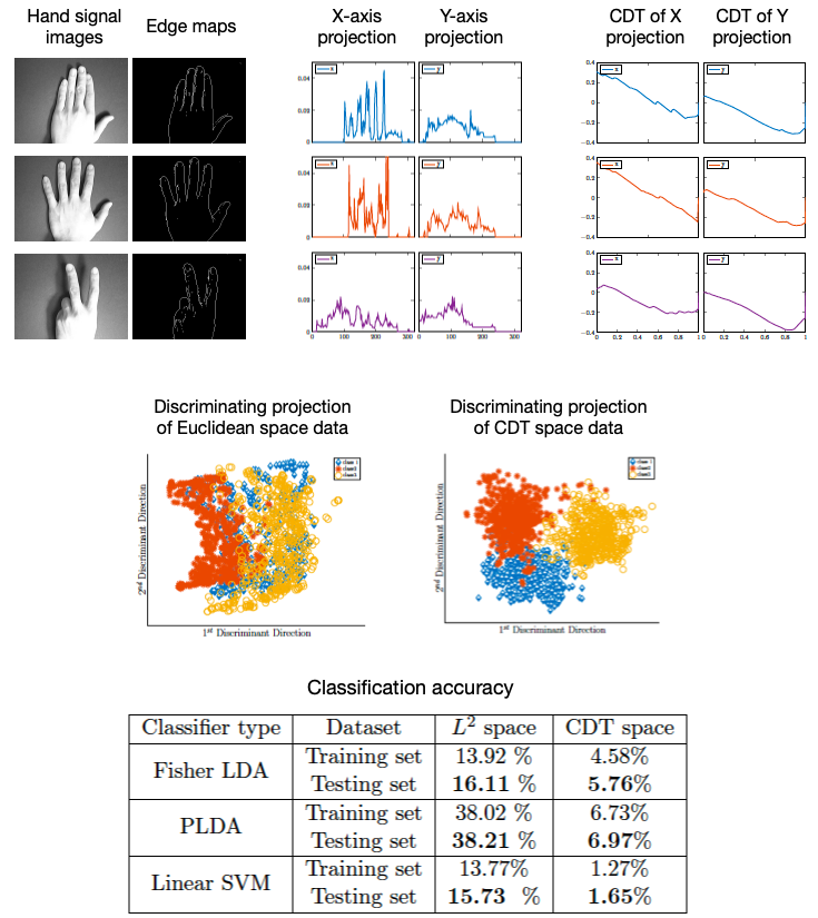
To illustrate some of the properties of the CDT, consider the task of building a hand signal interpretation system from image data. Sample hand signal images are shown in Figure 1, adapted from [30]. The goal is to build a data classification method that can automatically and accurately assign a label (sign) to a given image. Images are pre-processed so as to extract an edge map, and the and projections of the edge maps are computed (middle of first row in Figure 1). The CDT (modified by subtracting the identity function) of the projections are computed and shown in the right panel of the figure. The test data (both in signal and CDT domain) can be projected onto the most discriminant 2D subspace, computed with the P-LDA technique [9] on training data (middle row). From this it can be seen that the test data become more clearly linearly separable when represented in CDT domain. This visual impression is confirmed by classification results, shown in the bottom table, demonstrating the test data performance using three different linear classification methods. 11 1 The CDT defined in earlier work [30], and as appears in Figure 1, is defined as , with defined in equation (1).
1.1. Related work
The signal transformation described in this paper is related to the optimal transport metric (Wasserstein distance), as will be detailed below in section 3.2. Data analysis techniques that are based on optimal transport have gained popularity in the data science community. Machine learning methods based on optimal transport optimization have been developed in [25, 31]. Optimal transport methods have also been used in image processing for image alignment [5], image simulation [7], and domain adaptation [20]. Extensions of the optimal transport (Wasserstein) metric to unbalanced distributions have been proposed in [27, 16]. Inspired by [13] authors in [38] proposed a linear optimal transport metric for arbitrary (signed, unbalanced) signals. We also note a generalization of the Wasserstein distance to signed signals, similar to the one described in section 3, has been previously described in [21, 12].
1.2. Contributions
Although useful in many settings, the CDT framework described above has the limitation that the signals themselves must be positive for the entirety of their domain. While not prohibitive in certain settings [36], this limitation can hinder the application of the transform to signed functions that can be used to model more general signals and data.
Here we extend the CDT, originally designed for positive probability density functions, to general finite signed measures with no requirements on their total mass. For this reason, we name the new 1D signal transform introduced here as the signed cumulative distribution transform (SCDT). We define mathematical formulas for both the forward (analysis) and the inverse (synthesis) transformations. We describe some of the properties of the SCDT, including translation, scaling and composition. Through the use of an extended generative model, we also describe necessary and sufficient conditions whereby signal classes will be convex (and thus separable by a linear classifier). Finally, we define a distance based on this transform (a version of the distance appears earlier in [21, 12]), and demonstrate its application in signal data analysis and classification tasks. Python source code implementing the new transform is available through the PyTransKit package [40].
1.3. outline
2. Cumulative Distribution Transforms for Measures
In this section we extend the Cumulative Distribution Transform (CDT) to Radon measures on the extended real line . Because we use concepts related to the theory of transport, we start with an extension of CDT to probability measures. We then extend the CDT to include non-negative finite measures, and finally signed measures.
In the cumulative distribution transform for measures, a reference measure is fixed, and the transform of a measure relative to this fixed reference measure will be a non-decreasing function on denoted by .
2.1. The cumulative distribution transform on probability measures
Given any probability measure on , its Cumulative Distribution Function (CDF) is the function given by
| (3) |
The function is non-decreasing and right continuous on , and may not be invertible. However, a generalized inverse for such a function (in fact for any function) can be defined (see e.g., [11, 41]).
Definition 2.1.
For a function , the monotone generalized inverse of is the function defined as
In particular (since ),
The monotone generalized inverse has some remarkable properties. In particular, for any function , is a non-decreasing function on , and if is continuous and strictly increasing, then and its standard inverse coincide (see Appendix 6). Since the monotone generalized inverses are functions on , our measures will be defined on instead of . Those measures are characterized by their CDFs (which are functions on ) according to Proposition 6.1.
Given a reference measure , the cumulative distribution transform of a measure with respect to is defined as
| (4) |
where and are the CDFs of the respective measures. Under the assumption that does not give mass to atoms, the function (4) is the solution of the 1D optimal transport problem of Monge (see for example [41, 4]). In fact, the measure can be recovered by the push-forward of the measure by the function in (4) (see Theorem 2.2), i.e., for any Borel measurable set
| (5) |
If the reference measure and the target measure are continuous with respect to the Lebesgue measure with densities and , respectively, then equation (1) can be rewritten as follows
Therefore, equation (4) extends the definition of the CDT for functions as described by (1) to the case of probability measures on .
Writing (4) in operator notation as , we define the CDT operator by
| (6) |
where is the set of probability measures on and
| (7) |
is the set of non-decreasing functions with respect to . The next theorem states that the operator above is a bijection and hence can be viewed as a transform operator.
Theorem 2.2.
A measure defined on a Borel measurable subset can be considered as a measure on by extending it by zero. Equivalently, this extension can be written as the push-forward of by the inclusion map (). Thus, using this extension, we consider the set of probability measures defined on as a subset of , i.e., . Analogously, we will say that any measure satisfying and belongs to by considering its restriction. From these considerations, we obtain the following corollary of Theorem 2.2.
Corollary 2.3.
Remark 2.4.
In the corollary above, since is defined - and , we can consider the image of the transform operator to be the set
by considering the restriction for every .
Example 1.
This extension of the CDT to a transform for probability measures allows to consider the transform of a delta-function. Let be the Lebesgue measure on (that is, consider the uniform distribution). Let be the Dirac measure concentrated on . On the one hand, is zero on , the identity function on and on , and is the Heaviside step function (that is, the characteristic function of ). Therefore,
where
and
Thus,
| (8) |
In particular, , a.e.-. On the other hand, the push-forward of by the zero function
for every Borel set . Thus, .
2.2. Transform for positive finite measures with arbitrary total mass
The CDT for probability measures can be extended naturally to the case where the reference and the target are finite and positive Borel measures . Specifically, let be two finite positive measures such that is non-trivial, that is
If denotes the scaling function by the factor (i.e., ), then the transform of with respect to the reference is defined to be
| (9) |
and where
When , the non-decreasing function is simply the CDT of the probability measure with respect to the reference (see (4)), while the number is to keep track of the total mass of . The next theorem shows that (9) gives rise to a bijection and hence can be thought of as a transform. We abuse language and still call this transform the CDT since it will be clear from the context which transform is being used. Abusing notation by using again to denote the operator defined by we get the following bijection between the space of finite Borel measures and the set
| (10) |
where is as in (7), and .
Theorem 2.5.
If is a non-trivial finite positive measure on that does not give mass to atoms, then the operator is a bijection from to , whose inverse is given by
| (11) |
and the inverse of is the zero measure.
Defining , we get the following corollary.
Corollary 2.6.
Let be two Borel sets in and be a non-trivial finite positive Borel measure on that does not give mass to atoms. Then the CDT with respect to is a bijection from (the set of positive finite measures on ) to .
2.3. Transform for signed measures
To define the transform on signed measures, we use the Jordan decomposition of a signed measure [8]. Specifically, let be a signed, finite Borel measure on , with Jordan decomposition , then the image of with respect to a non-trivial positive measure is defined as
| (12) |
where are the CDTs of positive finite measures defined in (9). In particular, (see (10)). Denoting the set of finite signed measures on by , and defining
| (13) |
where denotes that and are mutually singular, we have the following theorem.
Theorem 2.7.
If is a non-trivial finite positive measure on that does not give mass to atoms, then the operator given in (12) is a bijection. Hence, is a transform.
Moreover, the inverse transform is given by
and the inverses of , , and are the measure , the measure , and the zero measure, respectively.
We call the operator given in (12) the Signed Cumulative Distribution Transform (SCDT).
As in previous subsections, restricting the measures to Borel sets and for and respectively, and defining
| (14) |
we obtain the following bijection result.
Corollary 2.8.
Let be two Borel sets in and be a non-trivial finite positive Borel measure on that does not give mass to atoms. Then the restriction of the transform to (the set of signed finite measures on ) is a bijection onto .
3. Properties and Applications
There are several properties of the CDT for positive PDFs that makes it a useful tool. The new transforms derived in this paper retain some of these useful properties. In particular, the computational example below, shows how these transforms can be useful in data classification.
3.1. Properties of the SCDT
In this section we list two of these properties: 1) the composition of property and 2) the convexification property.
The composition property relates the transform of a measure to that of a measure when their cumulations are related by a composition of functions. This property is useful for applications in which a set of signals is generated by a signal template that is modified by a transport-like phenomenon. Translations and scalings are examples of such classes [30] (see Figures 2 and 3).
Proposition 3.1.
(Composition property) Consider a finite positive reference measure which does not give mass to atoms. Let be a signed measure. Assume that is a strictly increasing surjection, and a signed measure such that . Then and the SCDT of with respect to is given by
when and If , , or then is given by , , respectively.
Corollary 3.2.
(Translation) If and are as above, and is a translation by , i.e. , then for such that , the SCDT of with respect to is given by . (See figure 2.)
Corollary 3.3.
(Dilation) If and are as above, is a dilation by , i.e. then for such that , the SCDT of with respect to is given by (See figure 3.)


It is also worth noting that in certain applications data sets can be rendered convex in the transform domain. For example, sets generated by translations of a template signal can have a complex geometry in the signal domain. However, it has a very simple convex structure in the transform domain as depicted in Figure 4. This convexification property is useful in classification problems since two disjoint convex data sets can be separated by a linear classifier. The following convexity property is a generalization of the convexity property that was proved in [32] for signals that consist of normalized, compactly supported, non-negative Lebesgue measurable functions.
Proposition 3.4.
(Convexity property) Let be a finite positive reference measure that does not give mass to atoms and let be a signed measure. Let be a subset of strictly increasing surjections on , and
| (15) |
Then, is convex for every if and only if is convex.
We remark that the set can be interpreted as an algebraic generative model for signal data. Here specifies a measure (signal) that can be considered as a template for its class, which is denoted by . The elements of are formed by the action of functions in , as in Proposition 3.4. For example, can be the set of all possible translations, or positive scalings. If is such that is convex, then the set is also convex. As explained in [32], is convex if is a convex group (numerous examples are described in [32]).

3.2. Metric
The Wasserstein distance in the space is intimately related to the distance in the transport transform domain [30, 41, 4]. This relation is useful in some applications since it render certain optimization problems involving the Wasserstein distance into standard least squares optimization problems. In this section, we will recall the definition of the Wasserstein distance for probability measures and its relation to the distance in the transform domain. We will extend this result using the generalized transport transforms of the previous section.
Definition 3.5 (Wasserstein distance).
Let be a Borel set endowed with the Euclidean distance. Let denote the subset of all probability measure on with finite second moment
The Wasserstein distance is defined as
| (16) |
where denotes the collection of all measures on with marginals and on the first and second factors respectively.
Proposition 3.6.
Let be a Borel set, and a reference measure that does not give mass to atoms. If , then
| (17) |
In particular, the transport transform is an isometry between with the Wasserstein metric and the image of the transport transform endowed with the metric.
3.3. Metric for and
Let and be the subsets of and , respectively, of measures having finite second moment. For that does not give mass to atoms, consider the Cartesian product endowed with the norm
For we define the following distance function:
| (18) |
In particular, from Proposition 3.6 it follows that for non-trivial measures , (18) coincides with
| (19) |
where is the Wasserstein distance defined in Equation (16). This identity and the definition of the transform when or are the zero measures, imply that does not depend on the choice of the reference . In particular, if is non-trivial and is the zero measure
which holds by applying Lemma 5.1 in the same way it is done in the proof of Proposition 3.6.
Using the Definition (18), becomes an isometry from to .
Analogously, by considering the space endowed with
we define
| (20) |
which endows with a distance on and which is independent from the choice of the reference . Indeed, using the Hahn-Jordan decomposition for , (20) is exactly
| (21) |
3.4. Applications
The CDT and SCDT have many applications in signal and image analysis which can be broadly categorized into signal estimation and detection (classification) problems. With regards to signal estimation, in [36] the authors applied the CDT to estimating parameters (time delay, frequency, chirp) pertaining to a measured signal. In that work, the CDT was used to ‘linearize’ the problem so that a global optimal estimate for signal parameters can be estimated in CDT space using a simple linear least squares technique. Here we show how the SCDT can be utilized to similarly facilitate the machine learning of classifiers by ‘linearizing’ the problem in transform space, as illustrated in Figure 4. To that end, we utilize the following property of the SCDT.
Let and be as defined in Proposition 3.4. The sets and can be interpreted as algebraic generative models for signal data. The theorem stated below becomes an easy consequence of Proposition 3.4 and the Hahn Banach separation theorem.
Theorem 3.7.
Let be a reference measure that does not give mass to atoms, be two signed measures, and be a convex set of strictly increasing bijections on . If are two non-empty, finite sets drawn from two disjoint generative models and , respectively, then the corresponding sets in SCDT space are linearly separable.
The theorem above states that so long as data is generated according to the algebraic generative model defined in Proposition 3.4, a training procedure using a linear classifier, using data in SCDT space, is a well-posed problem in the sense that there is a guarantee that a solution exists, although it may not be unique. The theorem does not state how to compute such linear function, rather it states that there will exist a linear classifier that will separate so long as and are disjoint.
To demonstrate the ability of the SCDT to render signal classes linearly separable we consider the problem of distinguishing signals of the kind demonstrated in Figure 5. Let signals be associated with the measures , and let , , and represent corresponding signal classes generated using the set of diffeomorphisms In short, three prototype signals are defined as a Gabor wave, a Sawtooth wave, and a Square wave, all multiplied by a Gaussian window function, respectively. These prototypes are randomly translated and scaled. For the computer simulations shown below, , and and are uniformly distributed in and respectively. A total of sample signals are generated with used for training and for testing. Randomly distributed Gaussian noise, with standard deviation of was added to each signal. The Fisher Linear Discriminant Analysis [1] computed using the sklearn python package [39], shows that classification accuracy on the test set using the data in original signal space is , while the test set accuracy of the same classification algorithm applied to signals in SCDT space is . The projections of the test set for both native signal space and SCDT space are shown in Figure 6 below. From these figures, and from the test set classification accuracy, we can see the SCDT significantly enhances the ability of a linear classifier to operate correctly.


4. Summary and Conclusions
This paper extends the Cumulative Distribution Transform [30] to signed measures of arbitrary mass, permitting the application of the technique to arbitrary one-dimensional signals. This extension significantly broadens the number of potential applications of the transform. The idea is based on viewing 1-D signals (measured data) as measures, and matching the measure corresponding to the signal to be transformed to a chosen reference measure. This matching is obtained using a push-forward of the reference measure by a function derived from the cumulations of the reference and signal measures. The operator that produces the push-forward function is what we call the Signed Cumulative Ditribution Transform (SCDT). Signed measures are handled using the Jordan decomposition, where the positive and negative portions are handled separately and independently. Theorem 2.7 shows that the mapping is bijective from the space of signed finite measures to the transform space. As such, the signed cumulative distribution transform described in this paper can be viewed as a mathematical signal representation method, with analytical forward and inverse operations, for arbitrary 1-D signals.
Following earlier work on the CDT [30], we also described several properties of the newly introduced SCDT. Proposition 3.1 states that for a strictly increasing surjective function, the SCDT of a signal (measure) satisfying will be related to the SCDT of via . Simple corollaries of the proposition include the signal translation and scaling properties 3.2, 3.3, describing that transformations that shift the signal along the independent variable ( in this case) become transformations that shift the signal in the dependent variable in transform space.
Proposition 3.1 (composition) and corollaries 3.2 (translation) and 3.3 (scaling/dilation) relate to the analysis of signals under rigid and non-rigid deformations (e.g., deformations in the independent variable time or space). Proposition 3.4 describes a generative model for classes of signals under the presence of deformations and describes the necessary and sufficient conditions for such classes to be convex in SCDT space. Section 3.3 describes a metric for 1D signals using the SCDT and Theorem 3.7 utilizes it, in combination with Proposition 3.4 and the Hahn-Banach separation theorem to establish sufficient conditions for linear separability of such signal classes in SCDT spaces. Finally, a computational example application of the technique to classifying signals under random translation and dilations using a simple linear classifier is shown.
The definition of the SCDT given in equations (12) and (13) is one of several possibilities. In the definition used here, we consider a positive, non trivial, reference measure to which the positive and negative components of the Jordan decomposition of the signal measure are matched. Another possibility would be to use a reference measure that also admits a decomposition , and then replace equation (12) with a similar version that matches the corresponding positive and negative parts:
with the range of the transform being
The properties of the transform (e.g. invertibility, composition, translation, dilation, convexity, etc.) under this alternative definition would remain the same, although the proofs would be slightly altered. Naturally, this alternative definition would require both and to be non-trivial.
In summary, this paper presents a new tool for representing arbitrary signals by matching their corresponding measures to a reference measure. As such, it enables the extraction and analysis of information related to rigid and non-rigid deformations of the signal, which are difficult to decode especially in nonlinear estimation and classification problems. Future work will include exploring the application of SCDT to a variety of signal estimation and classification problems, extension of the transform presented here to higher dimensional signals, as well as sampling, reconstruction, compression, and approximation problems.
5. Proofs of results
This section contains the proofs of our results. Some of the proofs rely on certain properties of the monotone generalized inverse whose properties and proofs are relegated to the appendix.
5.1. Proofs for Section 2
We start with several essential lemmas. The proof of Lemma 5.1 can be found in [18, Lemma 2.4] and also in the proof of [41, Corollary 2.2]. The proof of Lemmas 5.2 and 5.3 combine the proofs of [3, Theorem 3.1], [18, Theorem 2.5] and [41, Corollary 2.2]. We include them here for completeness, and because we extend them to . In what follows, we will use to denote the Lebesgue measure on .
Lemma 5.1.
Let be a probability measure that does not give mass to atoms, and let be its CDF (see (3)). Then . As a consequence, for every the set is negligible.
Proof.
Note that is continuous, as does not give mass to atoms. So, for all the set is closed, in particular for some with Now, for
Hence, as Borel measures, since they coincide on every interval , with . As a consequence, for all ,
∎
Lemma 5.2.
Let be two probability measures on , and assume that does not give mass to atoms. Then, is non-decreasing and satisfies .
Proof.
By Proposition 6.8(i), the function is non-decreasing. Thus, is non-decreasing since it is a composition of two non-decreasing functions. To show , we prove that
Then using from Lemma 5.1, and properties of the push-forward operator, we obtain the desired result. Indeed, for using Proposition 6.9 we get,
∎
Lemma 5.3.
Let be two probability measures on , and assume that does not give mass to atoms. If is a non-decreasing function such that , then -.
Proof.
Let be any non-decreasing function such that and assume, (possibly modifying on a countable set) that is right-continuous. Let
and notice that is at most countable (since we can index with a family of pairwise disjoint open intervals). We claim on . Indeed, for and we have
where last inequality follows from the fact that . Thus, we have that . Using the fact that and are non-decreasing and right continuous, we can apply Proposition 6.4(i) to get -. Taking we obtain for every . In particular, using Lemma 5.2 we get
But . Therefore, -a.e.
∎
5.1.1. Proofs of Theorem 2.2 and Corollary 2.3.
Proof of Theorem 2.2.
Injectivity holds since, by Lemma 5.3, if -a.e., then
For surjectivity, if is a non-decreasing -a.e function, then the push-forward of by is a probability measure on . By Lemma 5.3, for any probability measure , the transform is a unique non-decreasing function which satisfies . Therefore, -a.e., i.e. lies in the image of the transform. ∎
Proof of Corollary 2.3.
Note that , , and that is a bijection. Thus, the restriction is trivially one to one.
The surjectivity of follows from the surjectivity of if we can show that .
Indeed, given , since -a.e., we have that for each Borel set ,
Thus, . ∎
5.1.2. Proofs of Theorem 2.5 and Corollary 2.6
Proof of Theorem 2.5.
Note that if a function is a non-decreasing -a.e., it is also non-decreasing -a.e.
In order to prove injectivity, let and be two non-zero, finite positive measures on such that and . Hence, by Theorem 2.2, and we obtain . If and then from the Definition 9,
In order to prove surjectivity, consider the pair where is a function non-decreasing -a.e. and is a positive real number. Let , then is a finite positive Borel measure with since is a probability measure. In addition,
and by Lemma 5.3 it is the unique non-decreasing -a.e. function that satisfies
Thus, -a.e., and the inverse transform is given by
If , then, from Definition 9, it is the transform of the zero measure. ∎
5.1.3. Proofs of Theorem 2.7 and Corollary 2.8
Proofs of Theorem 2.7.
Given a signed measure , is well-defined since there exists only one pair of mutually singular positive measures, and , such that .
If , then and (where the operators should be understood from the context). Thus, injectivity follows by applying Theorem 2.2 separately on the positive and negative part.
In addition, given , since
In order to prove the surjectivity, consider . Define
| (22) |
For , since , then
Both measures, and , are positive measures and therefore they are a Jordan decomposition for , that is
In particular, and . By Theorem 2.2,
Thus, , and it is clear that the inverse transform is given by (22). Finally, if and (resp. and ) the proof reduces to the one of Theorem 2.5, and the point is reached by the zero measure by definition. ∎
5.2. Proofs of Section 3.1
The following Lemma is useful for the proofs of this section.
Lemma 5.4.
Let be two signed measures on such that for some strictly increasing bijection If is a Hahn decomposition of , then the set made by the pre-images is a Hahn decomposition of Thus,
Proof.
Throughout this proof, we will use the fact that if and satisfy the hypothesis of the Lemma 5.4, then, if and only if In particular, under the hypothesis of the Lemma,
Clearly, and Now we show that, is a positive set for i.e. for all - measurable sets
Since and is a bijection, there exists - measurable such that Thus, Analogously, we can show is a negative set for .
Now, we show A similar argument would follow for its negative counterpart.
∎
Proof of Proposition 3.1.
Using the relation, , we see that is a cumulation. Also, by definition of and , we have and by Lemma 5.4, we get, and In particular, . Since g is strictly increasing, and using Proposition 6.8, the SCDT of with respect to when and is given by
The cases when or can be done a similar fashion.
∎
We adopt a proof similar to the one in [32].
Proof of Proposition 3.4.
Given we consider as is (15). By the definition of , Proposition 3.1 and Theorem 2.7 we have that
| (23) |
Assume that is convex and fix . Let be two arbitrary elements in , that is, they are defined by and for (here we are using the characterization of measures according Proposition 6.1 from the Appendix). For any , applying Proposition 3.1 we have
In addition . Thus, is convex.
For the converse statement, let and . For , assuming that is convex we have that
Thus, by the characterization of given by (23) we obtain that coincides with a function in on the range of . Taking the family of target measures , where are Dirac measures centered at , and is defined by
and assuming convex for every , by Corollary 3.3 we can conclude that . Thus is convex. ∎
Proposition 3.6 and its proof are well-known [41]. We include them in this paper for readability and completeness.
Proof of Proposition 3.6.
Proof of Theorem 3.7.
Since are finite subsets of a normed space , their convex hulls , and are compact. In addition, since are subsets of the convex sets and , then , are also subsets of and . Finally, since and are disjoint and is one to one, we get that , and are disjoint non-empty convex and compact sets. By the Hahn-Banach Separation Theorem, they can be separated by a linear functional . In particular, separates . ∎
6. Appendix
6.1. Measures on
We recall that we are using the standard topology on , which is given by the standard topology on and a base of open neighborhoods of is and analogously for the point . Then, the Borel -algebra of is generated by , , with .
Proposition 6.1.
Let be a finite positive Borel measure on , then the cumulation of defined by for all , is non-decreasing, right-continuous, and
| (25) |
Conversely, for any right-continuous, non-decreasing function on satisfying (25), there is a unique finite positive Borel measure on such that
This is an extension of the so called Lebesgue-Stieltjes Measure.
Proof.
Direct part:
- •
is non-decreasing because given with , since ,
- •
(since is positive).
- •
Let
so is right-continuous on . Indeed, is right-continuous on : If there is nothing to prove. If , then for all therefore, .
For the converse part, let be a right-continuous, non-decreasing function satisfying (25). Denoting
define
Then, is non-decreasing, and therefore it is a measurable function. Notice that for each
In particular, if , and if because since the range of is a subset of .
We define
and, for each , we obtain
Notice that
The uniqueness of the measure is a consequence of the Carathéodory Extension Theorem, which asserts that any finite measure on an algebra extends in a unique way to a measure on the -algebra generated by . Indeed, the equation
implies that there is only one extension to the algebra of sets generated by and half-open intervals with , and so there is only one extension to the -algebra generated by these sets, which is . ∎
6.2. Monotone Generalised Inverse
In this section, we introduce the monotone generalized inverse for functions defined on the extended real line , and we provide some of its relevant properties. In particular, the monotone generalized inverse of any function is always non-decreasing, and if a function is continuous and strictly increasing then its monotone generalized inverse and its standard inverse coincide. This inverse and its properties are essential in defining and studying the transport transform on . It has already been introduced in connection to transport theory but only for functions on the real line [41], and some its properties are well-known [11]. However, we also need other properties that we derive in this appendix.
Definition 6.2.
For a function , the monotone generalized inverse of is the function defined as
In particular (since ),
The following properties of are used in this paper.
Remark 6.3.
For any function
- •
- •
If , then, .
- •
If is non-decreasing function on , then , then .
- •
If is non-decreasing function on , then
Proposition 6.4.
For any function
- (i)
- (ii)
Proof.
Since (i) follows from the definition of and (ii) is the contrapositive of (i).
∎
Proposition 6.5.
If is non-decreasing then
- (i)
- (ii)
- (iii)
Proof.
- (i)
Since and is non-decreasing, for any . Thus, (i) follows from definition of
- (ii)
If . Then, since is non-decreasing, for any such that . Thus,
- (iii)
From (i) and (ii) imply that if , then which is the contrapositive of (iii).
∎
Proposition 6.6.
If is right-continuous and non-decreasing then,
- (i)
- (ii)
- (iii)
Proof.
- (i)
If , by definition of infimum, for all , there exists such that and . Since, is non-decreasing and right-continuous, we have . If , then . Therefore, by right continuity at , . To see that (i) is not valid if we allow to be the domain of , consider any non-decreasing function that satisfies . Then we have that . However, .
- (ii)
If then by 6.5(ii), . If then by (i), which contradicts .
- (iii)
This implication is the contrapositive of (ii) above.
∎
Proposition 6.7.
If is strictly increasing then
| (26) |
Proof.
If then . Taking infimum on both sides we get . ∎
Proposition 6.8.
For a function the following hold:
- (i)
is right-continuous and non-decreasing.
- (ii)
if and only if is non-decreasing and right-continuous and . In other words, is non-decreasing and right-continuous if and only if .
- (iii)
If are non-decreasing, then .
- (iv)
Let be non-decreasing. If is strictly increasing, then .
Proof.
- (i)
Let be such that . Then
Taking the infimum on both sides we get that is non-decreasing.
Let be given. For , set and . Since is non-decreasing, if , then . Choose such that , and so small that . Then for any , we have
Thus,
Hence .
- (ii)
If , then, by Part (i), is non-decreasing and right-continuous. In addition by Remark 6.3, .
Conversely, let . Then using Proposition 6.4 (ii) we get set inclusion
Thus,
To prove that for all , first assume that there exists such that . For such an it must be that . Let be such that . Since is right-continuous, there exists such that for all . In addition since is non-decreasing and right-continuous, it follows from Proposition 6.6 (ii) that for all . This last inequality, by definition of , implies that But leading to a contradiction. Finally, since , and by assumption, we get part (ii).
- (iii)
- (iv)
∎
Proposition 6.9.
Let be cumulative distribution of a probability measure on . Then, for each
where is the Lebesgue measure.
Proof.
Since is cumulative distribution of a probability measure on , it is non-decreasing and right continuous. We then note that
Thus,
| (27) |
By Proposition 6.6 (iii) we get
References
- [1] Ronald Fisher “The use of multiple measurements in taxonomic problems” In Annals of eugenics 7.2 Wiley Online Library, 1936, pp. 179–188
- [2] Stéphane Mallat “A wavelet tour of signal processing” Academic press, 1999
- [3] Luigi Ambrosio “Lecture notes on optimal transport problems” In Mathematical aspects of evolving interfaces Springer, 2003, pp. 1–52
- [4] Cédric Villani “Topics in optimal transportation” American Mathematical Soc., 2003
- [5] Steven Haker, Lei Zhu, Allen Tannenbaum and Sigurd Angenent “Optimal mass transport for registration and warping” In International Journal of Computer Vision 60.3 Springer, 2004, pp. 225–240
- [6] David Kammler “A first course in Fourier analysis” Cambridge University Press, 2007
- [7] Lei Zhu, Yan Yang, Steven Haker and Allen Tannenbaum “An image morphing technique based on optimal mass preserving mapping” In IEEE Transactions on Image Processing 16.6 IEEE, 2007, pp. 1481–1495
- [8] H. Royden and P.M. Fitzpatrick “Real Analysis” Prentice Hall, 2010
- [9] Wei Wang, Yilin Mo, John Ozolek and Gustavo Rohde “Penalized fisher discriminant analysis and its application to image-based morphometry” In Pattern recognition letters 32.15 North-Holland, 2011, pp. 2128–2135
- [10] Stéphane Mallat “Group invariant scattering” In Communications on Pure and Applied Mathematics 65.10 Wiley Online Library, 2012, pp. 1331–1398
- [11] P. Embrechts and M. Hofert “A note on generalized inverses” In Math Meth Oper Res 77, 2013, pp. 423–432
- [12] Bjorn Engquist and Brittany Froese “Application of the Wasserstein metric to seismic signals” In arXiv preprint arXiv:1311.4581, 2013
- [13] Wei Wang et al. “A linear optimal transportation framework for quantifying and visualizing variations in sets of images” In International journal of computer vision 101.2 Springer, 2013, pp. 254–269
- [14] Saurav Basu, Soheil Kolouri and Gustavo Rohde “Detecting and visualizing cell phenotype differences from microscopy images using transport-based morphometry” In Proceedings of the National Academy of Sciences 111.9 National Acad Sciences, 2014, pp. 3448–3453
- [15] John Ozolek et al. “Accurate diagnosis of thyroid follicular lesions from nuclear morphology using supervised learning” In Medical image analysis 18.5 Elsevier, 2014, pp. 772–780
- [16] Lenaic Chizat, Gabriel Peyré, Bernhard Schmitzer and François-Xavier Vialard “Unbalanced optimal transport: geometry and Kantorovich formulation” In arXiv preprint arXiv:1508.05216, 2015
- [17] S. Kolouri and G.K. Rohde “Transport-Based Single Frame Super Resolution of Very Low Resolution Face Images” In Proc. IEEE CVPR, 2015, pp. 4876–4884
- [18] Filippo Santambrogio “Optimal transport for applied mathematicians” In Birkäuser, NY 55.58-63 Springer, 2015, pp. 94
- [19] Akif Tosun et al. “Detection of malignant mesothelioma using nuclear structure of mesothelial cells in effusion cytology specimens” In Cytometry Part A 87.4, 2015, pp. 326–333
- [20] Nicolas Courty, Rémi Flamary, Devis Tuia and Alain Rakotomamonjy “Optimal transport for domain adaptation” In IEEE transactions on pattern analysis and machine intelligence 39.9 IEEE, 2016, pp. 1853–1865
- [21] B. Engquist, B.. Froese and Y. Yang “Optimal transport for seismic full waveform inversion” In arXiv preprint arXiv:1602.01540, 2016
- [22] Soheil Kolouri, Se Park and Gustavo Rohde “The Radon cumulative distribution transform and its application to image classification” In IEEE transactions on image processing 25.2 IEEE, 2016, pp. 920–934
- [23] Soheil Kolouri, Yang Zou and Gustavo Rohde “Sliced wasserstein kernels for probability distributions” In Proceedings of the IEEE Conference on Computer Vision and Pattern Recognition, 2016, pp. 5258–5267
- [24] Soheil Kolouri, Akif Tosun, John Ozolek and Gustavo Rohde “A continuous linear optimal transport approach for pattern analysis in image datasets” In Pattern recognition 51 Pergamon, 2016, pp. 453–462
- [25] Martin Arjovsky, Soumith Chintala and Léon Bottou “Wasserstein generative adversarial networks” In International conference on machine learning, 2017, pp. 214–223 PMLR
- [26] Soheil Kolouri et al. “Optimal mass transport: Signal processing and machine-learning applications” In IEEE Signal Processing Magazine 34.4 IEEE, 2017, pp. 43–59
- [27] Matthew Thorpe et al. “A Transportation Distance for Signal Analysis” In Journal of Mathematical Imaging and Vision 59.2 Springer US, 2017, pp. 187–210
- [28] Shinjini Kundu et al. “Discovery and visualization of structural biomarkers from MRI using transport-based morphometry” In NeuroImage 167 Academic Press, 2018, pp. 256–275
- [29] Se Park et al. “De-multiplexing vortex modes in optical communications using transport-based pattern recognition” In Optics express 26.4 Optical Society of America, 2018, pp. 4004–4022
- [30] Se Park, Soheil Kolouri, Shinjini Kundu and Gustavo Rohde “The cumulative distribution transform and linear pattern classification” In Applied and Computational Harmonic Analysis 45.3 Elsevier, 2018, pp. 616–641
- [31] Soheil Kolouri et al. “Generalized sliced Wasserstein distances” In arXiv preprint arXiv:1902.00434, 2019
- [32] Akram Aldroubi, Shiying Li and Gustavo Rohde “Partitioning signal classes using transport transforms for data analysis and machine learning” In arXiv preprint arXiv:2008.03452, 2020
- [33] Tianji Cai, Junyi Cheng, Nathaniel Craig and Katy Craig “Linearized optimal transport for collider events” In Physical Review D 102.11 APS, 2020, pp. 116019
- [34] Shu-Wei Huang, Gustavo Rohde, Hao-Min Cheng and Shien-Fong Lin “Discretized Target Size Detection in Electrical Impedance Tomography Using Neural Network Classifier” In Journal of Nondestructive Evaluation 39.4 Springer US, 2020, pp. 1–9
- [35] Shinjini Kundu et al. “Enabling early detection of osteoarthritis from presymptomatic cartilage texture maps via transport-based learning” In Proceedings of the National Academy of Sciences 117.40 National Academy of Sciences, 2020, pp. 24709–24719
- [36] Abu Rubaiyat et al. “Parametric signal estimation using the cumulative distribution transform” In IEEE Transactions on Signal Processing IEEE, 2020
- [37] Mohammad Shifat-E-Rabbi et al. “Radon cumulative distribution transform subspace modeling for image classification” In arXiv preprint arXiv: 2004.03669, 2020
- [38] Tianji Cai, Junyi Cheng, Bernhard Schmitzer and Matthew Thorpe “The Linearized Hellinger–Kantorovich Distance” In arXiv preprint arXiv:2102.08807, 2021
- [39] Fabian Pedregosa “Scikit-learn: Machine Learning in Python”, http://jmlr.org/papers/v12/pedregosa11a.html
- [40] Gustavo. Rohde “PyTranskit”, https://github.com/rohdelab/PyTransKit
- [41] Matthew Thorpe “Introduction to Optimal Transport”, https://www.math.cmu.edu/~mthorpe/OTNotes