The Power Spectrum of Cosmological Number Densities

The galaxy volume number densities are important measures in cosmology as they give information about the evolving universe galaxy content and allow us to test cosmological models. This is so because they are able to connect theory and observation once different types of number densities are evaluated, both theoretically and observationally. Theoretically, these densities can be obtained once one chooses a cosmological spacetime geometry, usually the standard model given by the spatially homogeneous Friedmann-Lemaître-Robertson-Walker (FLRW) cosmology or, in a recent trend, the spatially inhomogeneous Lemaître-Tolman-Bondi cosmology as well (Iribarrem et al. 2013, 2014). Observationally, inasmuch as the galaxy luminosity function (LF) is a number density per unit luminosity, several authors have been systematically determining galaxy volume number densities using the LF derived from galaxy redshift surveys.

Comparing cosmological models with observations using number densities determined from LF parameters derived from observed data requires, however, some model connecting relativistic cosmology number counts theory to the LF astronomical data and practice. One way of pursuing this theoretical link was advanced by Ribeiro & Stoeger (2003, hereafter RS03) who used general relativistic theory to obtain specialized expressions capable of being applied to LF data. Albani et al. (2007, hereafter A07) and Iribarrem et al. (2012, hereafter Ir12) further extended such a link and applied the connecting expressions to the data of the Second Canadian Network for Observational Cosmology (CNOC2; see Lin et al.1999) and FORS Deep Field (FDF; see Gabasch et al.2004, 2006; hereafter G04 and G06 respectively) galaxy redshift surveys. Following the methodology advanced by Ribeiro (2005; see also Rangel Lemos & Ribeiro 2008) for number density definitions, where the adoption of cosmological distance measures is made explicit, A07 and Ir12 calculated the differential number density $\gamma$ and its integral counterpart $\gamma^{*}$ for various cosmological distances and used them to study the observational inhomogeneities in the relativistic radial distribution of galaxies (Ribeiro 2001) belonging to both datasets in the FLRW universe model. Their results indicated that observational inhomogeneities in the relativistic galaxy distribution can arise due to geometrical, past-light cone, effects even in the context of spatially homogeneous cosmologies.

Analyzes of the large-scale structure of the universe use, however, a complementary tool to examine such structures, the power spectrum (PS), which is basically a Fourier transform of the quantity under study. If galaxies form the basic units of a cosmological fluid described by a volume number density, this galactic fluid can also be considered as being composed of wave densities with different wave numbers. Then, the PS will give us the intensity, or power, in each component. This is essentially the PS analysis of the galaxy 2-point correlation function, as the information given by the PS is complementary to the correlation function. Various authors performed such an analysis (e.g. Sylos Labini et al.1998; Martínez & Saar 2002; Tegmark et al.2004, 2006; Gabrielli et al.2005) and showed that, in general, the PS behavior is a power-law. Since galaxy volume number densities were used by RS03, A07 and Ir12 to analyze the universe galaxy content and evolution, it is natural to expand these studies to include a PS analysis.

The goal of this work is to study the differential and integral number densities $\gamma$ and $\gamma^{\ast}$ in the wave number domain through the PS. This is achieved by performing Fourier transforms of both quantities. Using the relativistic analysis and results presented by Ir12, we computed the theoretical power spectra of $\gamma_{i}$ and $\gamma_{i}^{\ast}$ obtained using the cosmological distance $d_{i}$. Here the index $i$ stands for the adopted distance measure, namely the angular diameter distance $d_{\scriptscriptstyle A}$, also known as area distance, galaxy area distance $d_{\scriptscriptstyle G}$, luminosity distance $d_{\scriptscriptstyle L}$ and redshift distance $d_{z}$ $(i={\scriptstyle A},{\scriptstyle G},{\scriptstyle L}\,,{\scriptstyle Z})$. Observational values of the differential and integral densities computed with these distance measures, $[\gamma_{i}]_{{\textstyle{\scriptscriptstyle\mathrm{obs}}}}$ and $[\gamma_{i}^{\ast}]_{{\textstyle{\scriptscriptstyle\mathrm{obs}}}}$, were obtained using the results of Ir12, which employed the LF parameters derived by G04 and G06 from the FDF survey data. The analysis is also extended to include the power spectra of the ratio $\gamma/\gamma^{*}$ and of another quantity, named here as radial correlation $\Xi$, which is basically a radial function whose behavior in terms of $d_{i}$ bears some similarities to the 2-point correlation function (Ribeiro 1995).

The distance measures $d_{i}(z)$ were obtained in the cosmology adopted here: the FLRW model with non zero cosmological constant $\Lambda$ and parameter values equal to $\Omega_{m_{\scriptscriptstyle 0}}=0.3$, $\Omega_{\Lambda_{\scriptscriptstyle 0}}=0.7$ and $H_{0}=70\;\mbox{km}\;{\mbox{s}}^{-1}\;{\mbox{Mpc}}^{-1}$. The dataset studied here is the I-band selected luminosity functions of the FDF survey. Ir12 calculated observed differential number counts and then $[\gamma_{i}(z)]_{{\textstyle{\scriptscriptstyle\mathrm{obs}}}}$ and $[\gamma_{i}^{\ast}(z)]_{{\textstyle{\scriptscriptstyle\mathrm{obs}}}}$ using the absolute magnitudes, LF Schechter parameters and their respective redshift parametrization, all previously derived by G04 and G06 directly from the FDF data in eight bandwidths with a redshift range $0.5\leq z\leq 5.0$, for the blue bands (G04), and $0.45\leq z\leq 3.75$ for the red bands (G06). Those results allowed us to calculate the ratio $[\gamma_{i}/\gamma_{i}^{\ast}]_{{\textstyle{\scriptscriptstyle\mathrm{obs}}}}$ and the radial correlation $[\Xi_{i}(d_{i})]_{{\textstyle{\scriptscriptstyle\mathrm{obs}}}}$. Fourier transforms on these quantities provided their respective power spectra, $P_{k}[\gamma_{i}]_{{\textstyle{\scriptscriptstyle\mathrm{obs}}}}$, $P_{k}[\gamma_{i}^{\ast}]_{{\textstyle{\scriptscriptstyle\mathrm{obs}}}}$, $P_{k}[\gamma_{i}/\gamma_{i}^{\ast}]_{{\textstyle{\scriptscriptstyle\mathrm{obs}}}}$ and $P_{k}[\Xi_{i}]_{{\textstyle{\scriptscriptstyle\mathrm{obs}}}}$.

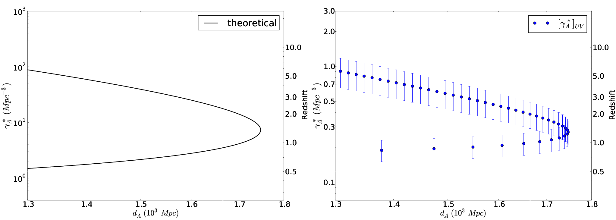
The results show that power spectra analyzes with the angular diameter distance $d_{\scriptscriptstyle A}$ is problematic, because each $d_{\scriptscriptstyle A}$ corresponds to two different values for $z$, since this distance starts from zero, grows to maximum and then tends to zero as $z\rightarrow\infty$. This maximum $d_{\scriptscriptstyle A}$ value is the only one with unique redshift. Due to these features the results obtained with $d_{\scriptscriptstyle A}$ turn out to be problematic in terms of interpretation.

We were also able to reproduce the preliminary results of Ribeiro (1995) regarding the radial correlation, confirming its dependency with the sample size and finding out that its respective PS is also sample size dependent. The best results, however, were obtained with the power spectra of the differential and integral densities using $d_{\scriptscriptstyle L}$ and $d_{z}$, which show a behavior bearing similarities, even at wave number values, with the 2-point correlation function PS. This suggests that PS analysis of number densities can also be a complementary tool for large-scale structure studies.

The plan of the paper is as follows. In §2 the basic quantities used in this paper are presented, as well as the expressions required in their calculation. §3 specializes the previously discussed general quantities to the FLRW cosmological model and shows how the luminosity function parameters of the FDF survey are used to calculated the desired observational expressions. §4 presents both the theoretical and observation results of all quantities discussed here, as well as their respective power spectra, and §5 presents our conclusions.

This section defines the basic quantities and expressions necessary for the PS analysis discussed here. Although they have already been introduced in previous papers (Ribeiro 1995, 2005; Rangel Lemos & Ribeiro 2008; A07; Ir12), one can find below a few additional clarifying remarks.

The quantities defined above are general, that is, valid for any cosmological model. In this section we shall adopt the FLRW cosmology and calculate them in this specific universe model, as well as using galaxy redshift survey observations.

As a simple examination of the equations above shows, we only require cosmologic specific expressions for $d_{i}(z)$, $\mathrm{d}(d_{i})/\mathrm{d}z$, $N(z)$, $\mathrm{d}N/\mathrm{d}z$, $[N]_{{\textstyle{\scriptscriptstyle\mathrm{obs}}}}$ and $[\mathrm{d}N(z)/\mathrm{d}z]_{{\textstyle{\scriptscriptstyle\mathrm{obs}}}}$. The first four quantities are theoretical and come from the chosen spacetime geometry, whereas the last two ones come from a combination of theoretical and observational results, as we shall see next.

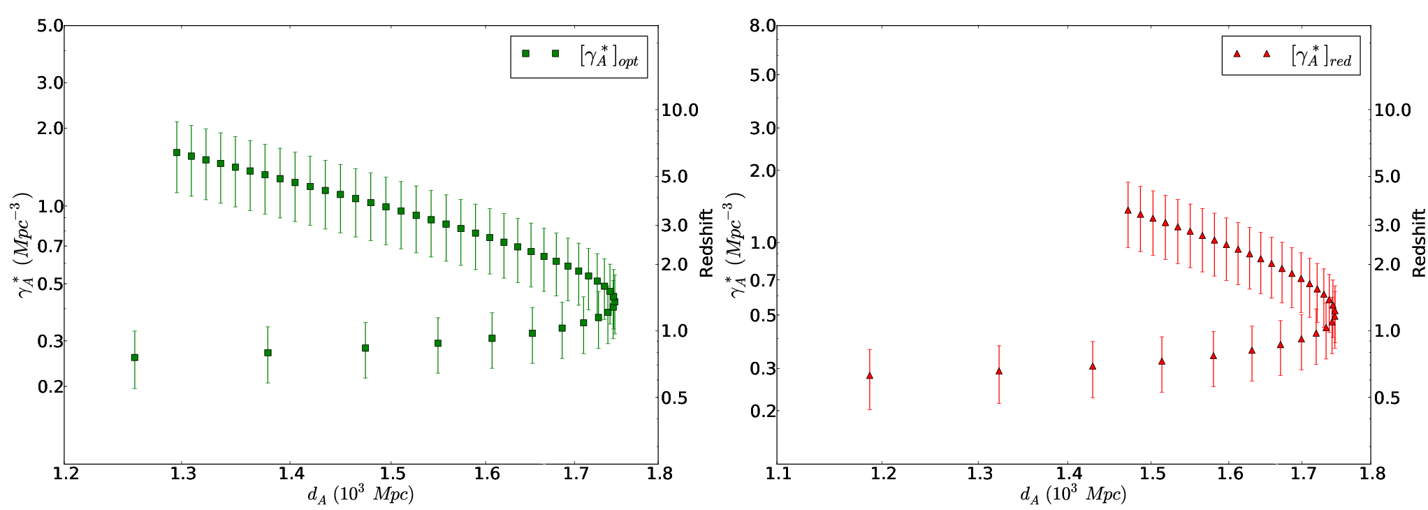
The observational values of the differential number counts $[\mathrm{d}N/\mathrm{d}z]_{{\textstyle{\scriptscriptstyle\mathrm{obs}}}}$ for all filters in the dataset allowed us to evaluate the observational differential number densities $[\gamma]_{{\textstyle{\scriptscriptstyle\mathrm{obs}}}}$ for the FLRW cosmology distance measures discussed above by simply replacing $\mathrm{d}N/\mathrm{d}z$ with $[\mathrm{d}N/\mathrm{d}z]_{{\textstyle{\scriptscriptstyle\mathrm{obs}}}}$ in Eq. (4). The dependence of these densities on the distance definitions are shown in Fig. 2. Similarly, the observational values of the integral densities $[\gamma^{\ast}]_{{\textstyle{\scriptscriptstyle\mathrm{obs}}}}$ were obtained by replacing $N$ with $[N]_{{\textstyle{\scriptscriptstyle\mathrm{obs}}}}$ in Eq. (5). The results are shown in Fig. 3.

The differential density constructed with the area distance $d_{\scriptscriptstyle A}$ becomes discontinuous at $z\approx 1.6$ because $d_{\scriptscriptstyle A}$ reaches a maximum at that redshift and, therefore, its derivative with respect to $z$ vanishes, rendering $[\gamma_{\scriptscriptstyle A}]_{{\textstyle{\scriptscriptstyle\mathrm{obs}}}}$ undefined. In addition, due to this maximum $[\gamma^{\ast}_{\scriptscriptstyle A}]_{{\textstyle{\scriptscriptstyle\mathrm{obs}}}}$ has a curious turn around in $d_{\scriptscriptstyle A}$ at $z\approx 1.6$, as shown in Fig. 3. Nevertheless, Fig. 4 shows that such a curious behavior does not occur when the integral density $\gamma^{\ast}_{\scriptscriptstyle A}$ is plotted in terms of $z$, which in this case keeps on increasing. This is due to the fact that each $d_{\scriptscriptstyle A}$ corresponds to two redshift values (see Fig. 1), but since each $z$ produces only one $\gamma_{\scriptscriptstyle A}^{\ast}$, each $d_{\scriptscriptstyle A}$ generates then two values for $z$ and $\gamma_{\scriptscriptstyle A}^{\ast}$. The single point where this behavior is absent is when $d_{\scriptscriptstyle A}$ reaches its maximum, which corresponds to single values for $d_{\scriptscriptstyle A}$, $z$ and $\gamma_{\scriptscriptstyle A}^{\ast}$. This effect is better visualized in Fig. 5 where a redshift scale was added to the right side of each plot.

Fig. 6 shows the PS of the FDF observational differential densities ${P_{k}}[\gamma_{i}]_{{\textstyle{\scriptscriptstyle\mathrm{obs}}}}$ and their theoretical counterparts plotted against the wave number $k_{i}$ and the redshift. The observational points were determined by means of the combined UV, optical and red bands in the G04 and G06 dataset. It is clear from the graphs that $P_{k}[\gamma_{\scriptscriptstyle A}]_{{\textstyle{\scriptscriptstyle\mathrm{obs}}}}$ possesses an odd behavior due to its discontinuity at $z\approx 1.6$, bearing no resemblance to the PS of the two-point correlation function, whereas the other power spectra $P_{k}[\gamma_{i={\scriptscriptstyle G,\;L,\;Z}}]_{{\textstyle{\scriptscriptstyle\mathrm{obs}}}}$ show a similar behavior to the two-point correlation function PS as presented by Tegmark et al. (2004, Fig. 38). We note that these authors calculated the two-point correlation function PS using different types of data, such as cosmic background radiation, galaxies, clusters of galaxies, lensing and Lyman alpha forest. Nevertheless, their general PS behavior is basically similar to ours, apart from the one calculated with $d_{\scriptscriptstyle A}$.

The PS of the observational integral densities in the UV, optical and red combined bands versus the wave number and the redshift are shown in Fig. 7. We note that $P_{k}\left[\gamma^{\ast}_{i={\scriptscriptstyle G,\;L,\;Z}}\right]_{{\textstyle{\scriptscriptstyle\mathrm{obs}}}}$ differ from from $P_{k}[\gamma_{i={\scriptscriptstyle G,\;L,\;Z}}]_{{\textstyle{\scriptscriptstyle\mathrm{obs}}}}$ shown in the previous figure only at small wave number values or, equivalently, at higher redshifts. Such difference occurs because the differential densities measure the rate of growth in number counts since $\gamma_{i}\propto\mathrm{d}N/\mathrm{d}z$, whereas $\gamma^{\ast}_{i}\propto N$ (see Eqs. 4 and 5). As $N$ is a cumulative quantity, it can only increase or remain constant, while $\mathrm{d}N/\mathrm{d}z$ increases, reaches a maximum and then decreases at scales dependent on the ratio of increase in $N$. Clearly the declining behavior of $\mathrm{d}N/\mathrm{d}z$ will occur at higher values of $z$, beyond its maximum, leading the decline in $\gamma$ to become even more pronounced at those scales. In addition, by measuring the rate of growth in number counts, $\gamma$ is more sensitive to local fluctuations due to noisy data. Thus, the steeper decline detected in the slopes of $P_{k}[\gamma_{i={\scriptscriptstyle G,\;L,\;Z}}]_{{\textstyle{\scriptscriptstyle\mathrm{obs}}}}$ at small wave numbers as compared to those at $P_{k}\left[\gamma^{\ast}_{i={\scriptscriptstyle G,\;L,\;Z}}\right]_{{\textstyle{\scriptscriptstyle\mathrm{obs}}}}$ can be attributed to these distortion effects at the redshift limits of the sample.

As discussed above, the radial correlation $\Xi_{i}(d_{i})$ proposed by Ribeiro (1995) was then studied in the Einstein-de Sitter model, but only with the luminosity distance. Here we extend the analysis of Eq. (7) to the galaxy area distance and redshift distance in the FLRW model with $\Omega_{m}=0.3$ and $\Omega_{\Lambda}=0.7$. These results are shown in Fig. 8 where one can see that, similarly to the Einstein-de Sitter cosmology, the amplitude of $[\Xi_{\scriptscriptstyle L}]_{{\textstyle{\scriptscriptstyle\mathrm{obs}}}}$ in the FLRW model also depends on the sample size. The extension of these results to $d_{z}$ and $d_{\scriptscriptstyle G}$ are presented in Fig. 9, where different sample sizes were used, confirming thus such a dependence. Due to the pathological behavior of $d_{\scriptscriptstyle A}$, $[\Xi_{\scriptscriptstyle A}]_{{\textstyle{\scriptscriptstyle\mathrm{obs}}}}$ was not evaluated.

Once in possession of the $[\Xi_{i={\scriptscriptstyle G,\;L,\;Z}}]_{{\textstyle{\scriptscriptstyle\mathrm{obs}}}}$ computations for the FDF dataset, it is natural to look at the behavior of their respective power spectrum. Fig. 10 shows such PS results, where one can see a distortion at small wave numbers probably caused by the subtraction of one in Eq. (7). To see if that is actually the reason behind this distortion, we evaluated the PS of the ratio $\gamma/\gamma^{*}$ for $d_{\scriptscriptstyle L}$, $d_{z}$ and $d_{\scriptscriptstyle G}$. Graphs of these quantities are shown in Fig. 11 where we can clearly see the absence of the previous distortion. This means that as far the observed PS for the radial correlation $P_{k}[\Xi_{i}]_{{\textstyle{\scriptscriptstyle\mathrm{obs}}}}$ is concerned, this is better calculated if one redefines $\Xi_{i}$ in Eq. (7) as follows,

Finally, the PS of the ratio $\gamma/\gamma^{*}$ for the area distance are shown in Fig. 12 where the discontinuity in $\gamma_{\scriptscriptstyle A}$ and $[\gamma_{\scriptscriptstyle A}]_{{\textstyle{\scriptscriptstyle\mathrm{obs}}}}$ translates themselves to discontinuous behavior for $P_{k}[\gamma_{\scriptscriptstyle A}/\gamma_{\scriptscriptstyle A}^{\ast}]_{{\textstyle{\scriptscriptstyle\mathrm{obs}}}}$.

In this paper we have studied the theoretical and observational power spectrum of the differential and integral galaxy volume number densities $\gamma$ and $\gamma^{\ast}$ using various relativistic cosmology distance measures $d_{i}$, namely the angular diameter distance $d_{\scriptscriptstyle A}$, galaxy area distance $d_{\scriptscriptstyle G}$, luminosity distance $d_{\scriptscriptstyle L}$ and redshift distance $d_{z}$ $(i={\scriptstyle A},{\scriptstyle G},{\scriptstyle L}\,,{\scriptstyle Z})$. The cosmology adopted here is the FLRW model with non zero cosmological constant $\Lambda$ having $\Omega_{m_{\scriptscriptstyle 0}}=0.3$, $\Omega_{\Lambda_{\scriptscriptstyle 0}}=0.7$ and $H_{0}=70\;\mbox{ km}\;{\mbox{s}}^{-1}\;{\mbox{Mpc}}^{-1}$. Observational results were obtained by following the framework that connects the relativistic cosmology number counts theory with the astronomical data extracted from the galaxy luminosity function (LF), as proposed by Ribeiro & Stoeger (2003) and further developed by Albani et al.(2007) and Iribarrem et al.(2012). This framework uses the LF parameters of the FDF galaxy survey provided by Gabasch et al.(2004, 2006) in order to calculate the observed differential number counts $[\mathrm{d}N/\mathrm{d}z]_{{\textstyle{\scriptscriptstyle\mathrm{obs}}}}$ required to build the observational densities $[\gamma_{i}]_{{\textstyle{\scriptscriptstyle\mathrm{obs}}}}$ and $[\gamma^{\ast}_{i}]_{{\textstyle{\scriptscriptstyle\mathrm{obs}}}}$. The observational results were produced in the combined red, blue optical and UV bands in the redshift range $0.5\leq z\leq 5.0$.

The PS of the galaxy volume number densities were obtained directly from both $[\gamma_{i}]_{{\textstyle{\scriptscriptstyle\mathrm{obs}}}}$ and $[\gamma^{\ast}_{i}]_{{\textstyle{\scriptscriptstyle\mathrm{obs}}}}$ and two other combinations of these quantities, namely the ratio $[\gamma_{i}/\gamma^{\ast}_{i}]_{{\textstyle{\scriptscriptstyle\mathrm{obs}}}}$ and the radial correlation $[\Xi_{i}]_{{\textstyle{\scriptscriptstyle\mathrm{obs}}}}$ which mixes up these two densities in a way that they can be discussed in terms of the sample size and each distance measure used above. Therefore, our analysis was able to compute $P_{k}[\gamma_{i}]_{{\textstyle{\scriptscriptstyle\mathrm{obs}}}}$, $P_{k}[\gamma_{i}^{\ast}]_{{\textstyle{\scriptscriptstyle\mathrm{obs}}}}$, $P_{k}[\gamma_{i}/\gamma_{i}^{\ast}]_{{\textstyle{\scriptscriptstyle\mathrm{obs}}}}$ and $P_{k}[\Xi_{i}]_{{\textstyle{\scriptscriptstyle\mathrm{obs}}}}$.

The results show that the graphs for $P_{k}[\gamma_{i={\scriptscriptstyle G,\;L,\;Z}}]_{{\textstyle{\scriptscriptstyle\mathrm{obs}}}}$, $P_{k}\left[\gamma_{i={\scriptscriptstyle G,\;L,\;Z}}^{\ast}\right]_{{\textstyle{\scriptscriptstyle\mathrm{obs}}}}$ and $P_{k}\left[{(\gamma_{i}/\gamma_{i}^{\ast})}_{i={\scriptscriptstyle G,\;L,\;Z}}\right]_{{\textstyle{\scriptscriptstyle\mathrm{obs}}}}$ have similar behavior for larger wave numbers, but the first differs from the other two at small wave numbers. Both $P_{k}\left[\gamma_{i={\scriptscriptstyle G,\;L,\;Z}}^{\ast}\right]_{{\textstyle{\scriptscriptstyle\mathrm{obs}}}}$ and $P_{k}\left[{(\gamma_{i}/\gamma_{i}^{\ast})}_{i={\scriptscriptstyle G,\;L,\;Z}}\right]_{{\textstyle{\scriptscriptstyle\mathrm{obs}}}}$ have general power-law behavior, whereas $P_{k}[\gamma_{i={\scriptscriptstyle G,\;L,\;Z}}]_{{\textstyle{\scriptscriptstyle\mathrm{obs}}}}$ behaves more similarly to the PS derived from the 2-point correlation function (see Fig. 38 of Tegmark et al. 2004) having a more pronounced decline at very small wave numbers.

The PS analysis using $d_{\scriptscriptstyle A}$ is problematic because this distance measure starts increasing, reaches a maximum and then decreases, resulting in a discontinuous $[\gamma_{\scriptscriptstyle A}]_{{\textstyle{\scriptscriptstyle\mathrm{obs}}}}$ at $z\approx 1.6$. Therefore, both $P_{k}[\gamma_{\scriptscriptstyle A}]_{{\textstyle{\scriptscriptstyle\mathrm{obs}}}}$ and $P_{k}\left[{\gamma_{\scriptscriptstyle A}/\gamma_{\scriptscriptstyle A}^{\ast}}\right]_{{\textstyle{\scriptscriptstyle\mathrm{obs}}}}$ also present discontinuities. $P_{k}[\gamma^{\ast}_{\scriptscriptstyle A}]_{{\textstyle{\scriptscriptstyle\mathrm{obs}}}}$ is, however, continuous, but has a minimum wave number value just as $d_{\scriptscriptstyle A}$ has a maximum.

The radial correlation ${\Xi_{i}}$, a quantity defined to possibly exhibit sample dependence in observational values, actually showed such a dependence for $[\Xi_{i={\scriptscriptstyle G,\;L,\;Z}}]_{{\textstyle{\scriptscriptstyle\mathrm{obs}}}}$, confirming a previous theoretical prediction made by using only the luminosity distance $d_{\scriptscriptstyle L}$ (Ribeiro 1995). Nevertheless, their respective PS $P_{k}\left[\Xi_{i={\scriptscriptstyle G,\;L,\;Z}}\right]_{{\textstyle{\scriptscriptstyle\mathrm{obs}}}}$ present some strong distortions.

In summary, the study presented here suggests that the PS analysis of the galaxy number densities can be considered as a complementary tools for studies of the large-scale galaxy distribution. That may be particularly the case of models describing the galaxy distribution as a fractal system, as advanced by Conde-Saavedra et al. (2015) and Teles et al. (2021), because these works showed that both $\gamma_{i}$ and $\gamma_{i}^{\ast}$ are essential tools for the fractal characterization of the galaxy distribution. This is particularly the case because these densities present decaying power-law behavior for $i=({\scriptstyle G},{\scriptstyle L},{\scriptstyle Z})$ at increasing distances, as shown in Figs. 2 and 3. Since their respetive power spectra also behave mostly as decaying power-laws for larger wave numbers, as seen in Figs. 6 and 7, as well as with the radial correlations in Fig. 9 and their redefined power spectra (Eq. 36) as shown in Fig. 11, these quantities provide additional tools for probing the large-scale galaxy distribution in the universe.

All data generated or analysed during this study are included in this published article.