Formally Verified Next-Generation Airborne Collision Avoidance Games in ACAS XCCS: Theory of computation Timed and hybrid modelsCCS: Theory of computation Modal and temporal logicsCCS: Theory of computation Programming logicCCS: Computer systems organization Embedded systems
Abstract.
The design of aircraft collision avoidance algorithms is a subtle but important challenge that merits the need for provable safety guarantees. Obtaining such guarantees is nontrivial given the unpredictability of the interplay of the intruder aircraft decisions, the ownship pilot reactions, and the subtlety of the continuous motion dynamics of aircraft. Existing collision avoidance systems, such as TCAS and the Next-Generation Airborne Collision Avoidance System ACAS X, have been analyzed assuming severe restrictions on the intruder’s flight maneuvers, limiting their safety guarantees in real-world scenarios where the intruder may change its course.
This work takes a conceptually significant and practically relevant departure from existing ACAS X models by generalizing them to hybrid games with first-class representations of the ownship and intruder decisions coming from two independent players, enabling significantly advanced predictive power. By proving the existence of winning strategies for the resulting Adversarial ACAS X in differential game logic, collision-freedom is established for the rich encounters of ownship and intruder aircraft with independent decisions along differential equations for flight paths with evolving vertical/horizontal velocities. We present three classes of models of increasing complexity: single-advisory infinite-time models, bounded time models, and infinite time, multi-advisory models. Within each class of models, we identify symbolic conditions and prove that there then always is a possible ownship maneuver that will prevent a collision between the two aircraft.
Keywords:
Airborne Collision Avoidance, ACAS X, theorem proving, hybrid games, differential game logic1. Introduction
Mid-air aircraft collisions are a fundamental responsibility of pilots and air traffic controllers to avoid, but their likelihood only increases as air space gets more congested and Unmanned Aerial Vehicles become more prevalent. The first onboard collision avoidance system, known as Traffic Alert and Collision Avoidance System (TCAS), was developed in the 1970s and has successfully prevented several mid-air collisions. However, this system is not perfect; one particular failure of TCAS occurred in the 2002 Überlingen crash, where two airplanes collided despite having received instructions by their TCAS systems onboard. Tragedies like this underscore the importance of continued research into developing and formally verifying onboard collision avoidance systems.
Most of the time, when aircraft are on a collision course, they are detected and resolved in advance by either the pilots or flight directors of the Air Route Traffic Control Centers. However, in rare scenarios where conflicting flight paths were not detected early enough and two aircraft are on an immediate collision course, collision avoidance maneuvers must be performed as a last resort. With little time to determine and perform the necessary maneuvers to avoid collision, it is imperative to ensure the safety of these collision avoidance maneuvers in advance using formal verification under all reasonable flight circumstances to ensure that no midair collisions happen.
The TCAS, and the more recent ACAS X, collision avoidance systems developed by the Federal Aviation Association (FAA) give vertical ascent/descent advisories when an aircraft is encountering an intruder with which it is at risk of colliding (Office 2014b). The goal of ACAS X is to prevent Near Mid-Air Collisions (NMACs), dangerous situations where two aircraft come within ft horizontally and ft vertically of each other (Kochenderfer et al. 2012). These variables and describe the radius and height, respectively, of a puck surrounding the aircraft, into which no other aircraft should enter.
Previous work explores formal verification of ACAS X when the intruder aircraft is moving at a constant horizontal and vertical velocity (Jeannin et al. 2017). This assumption is rigid and does not take into account the potential maneuvers that the intruder may perform. This article takes a conceptually significant departure by generalizing formally verified ACAS X models from hybrid systems to hybrid games, owing to the fundamental observation that, despite best intent, the actions of the ownship and intruder aircraft may interfere with one another since they are resolved by different pilots with different situational awareness facing a challenging safety hazard. This generalization is of practical relevance for the predictive power of verified ACAS X models but requires a fundamental shift in reasoning using differential game logic for hybrid games (Platzer 2015; Platzer 2017b; Platzer 2018). Hybrid systems are fundamentally single player. Only hybrid games can faithfully represent a dynamics where different pilots of different aircraft may independently reach different decisions at different times with different consequences on the flight of the two aircraft. While all pilots share the intent of avoiding collisions, only hybrid games accurately reflect that their decisions may, nevertheless, interfere, because the pilots chose different means to avoid collisions that may conflict.
1.1. Airborne Collision Avoidance System ACAS X
ACAS X tracks the position and velocity of the ownship and intruders in its vicinity using a variety of sensors to compute its collision avoidance advisories (Office 2014a). An advisory alerts the pilot with an audio-visual message and requests that she either maintain her vertical speed, or accelerate towards a new desired vertical speed. An advisory is issued only when a potential collision is identified, otherwise the system stays quiet to avoid distracting the pilot (Office 2014b). Advisories apply only in the vertical direction, not the horizontal direction, and only apply to the aircraft’s climb rate.
![[Uncaptioned image]](2106.02030v2/Table-1-no-MTLO.png)
Table 1 gives all of the 16 possible advisories issued by ACAS X, plus Clear-of-Conflict (COC), which indicates that no action is necessary. These advisories vary in the extremeness of the action; a less extreme advisory like Do Not Descend (DND) only requires that the ownship does not, as the name suggests, descend past its current altitude. A more extreme advisory like SCL2500 requires the ownship to reach a climb rate of at least 2,500 ft/min. Advisories can also be either lower bounds, like SCL2500, or upper bounds, like DNC2000 which requires that the ownship not exceed a climb rate of more than 2000 ft/min. The FAA assumes that in order for the pilot to achieve the desired climb or descend rate, she does so by following a vertical acceleration of strength at least (referred to as the positive constant ) (Kochenderfer et al. 2008), an assumption which will be pertinent later.
These advisories result from an estimation of the pilot’s optimal course of action, calculated by linearly interpolating a precomputed table of scores for various actions. The domain of this table includes parameters describing the state of the encounter, while its range gives scores for each possible action (Kochenderfer et al. 2008). This table is constructed from a Markov Decision Process which approximates the dynamics of the system on a discretized grid of the state space. From there, dynamic programming is used to optimize the table through maximizing the expected value of each event over all future outcomes for each action (Kochenderfer et al. 2008). These expected values approximately map to different outcomes: Near Mid-Air Collisions (NMACs), for example, correspond to large negative values, while issuing advisories corresponds to small negative values. The ACAS X system then uses a multilinear interpolation of grid points and heuristics to choose the action with the greatest expected value given the particular circumstances surrounding the ownship’s current flight conditions.
1.2. Formally Verified Safe Regions and Hybrid Game Logic
Previous work (Jeannin et al. 2015; Jeannin et al. 2017) applied hybrid systems to the formal verification process, a natural application given the combination of discrete advisories and continuous dynamics of an aircraft using ACAS X. While direct verification of the ACAS X implementation is infeasible given the complexity of ACAS X (whose core lookup table defines 29,212,664 interpolation regions in a 5-dimensional state-space giving rise to at least half a trillion cases to consider), this work cut down the complexity with the concept of safe regions. A region is proven safe if for all possible ownship positions and velocities within the region, an NMAC with the intruder will never occur. Thus, if ACAS X issues an advisory, and following this advisory in any permitted way always keeps the ownship within our safe region, then this advisory is guaranteed to maintain safety. These regions comprise fully symbolic parameters like , making them easily adaptable to new ACAS X versions.
In this work, we continue with the identification of safe regions to prove safety of the overall system, but we make the important change of applying hybrid games, rather than hybrid systems, in our formal verification of ACAS X. This change is motivated by the goal to model scenarios in which the intruder is maneuvering, such as being able to change its horizontal direction or vertical velocity. Where hybrid systems only allow one actor in the system to resolve decisions, hybrid games give multiple actors independent decision-making ability.
More specifically, the models presented in this article are rephrased using Differential Game Logic dGL (Platzer 2015; Platzer 2017b; Platzer 2018) from the Differential Dynamic Logic dL (Platzer 2008; Platzer 2010; Platzer 2012; Platzer 2017a; Platzer 2018) of previous work. dGL is an extension of dL, so it also supports discrete assignments, control structures, and following of differential equations to represent pilot decisions, trajectory requirements, and aircraft dynamics, respectively. However, dGL can also represent adversarial dynamics, meaning dGL can express two different players in a game scenario making independent decisions that may interfere. We make crucial use of this multi-player dynamics in our ACAS X game models in order to enable both aircraft to maneuver independently. Contrast this flexibility with hybrid systems models of ACAS X (Jeannin et al. 2015; Jeannin et al. 2017), which are necessarily limited to a single fixed policy for the intruder (the intruder cannot maneuver but is assumed to follow a straight line trajectory in prior ACAS X work (Jeannin et al. 2015; Jeannin et al. 2017)).
In the context of collision avoidance, one can think of the ownship as being a good-faith actor attempting to avoid collision, while the intruder is able to act independently in ways that, perhaps out of confusion, may interfere with the safety of the system. Since these two players follow independent intent, dGL works perfectly in this scenario to express these adversarial dynamics.

Of course, in the real world intruder will not actively attempt to collide with the ownship, but if the ownship’s goal is to avoid collision no matter the actions of the intruder, it is important to consider even the worst-case maneuvers that the intruder may perform. Notably, our ACAS X game model considers the case where the intruder’s actions may interfere with the safety of the system but does not assume they will. Indeed, the actions that the ownship pilot’s winning strategies for the ACAS X game needs to take to avoid collision are less extreme when the intruder pilot reaches helpful decisions and more extreme otherwise, see Fig. 1. dGL is implemented in the theorem prover KeYmaera X (Fulton et al. 2015), with which we verify our safe regions with respect to our models.
As far as we know, this is the first work to apply hybrid games to the problem of aircraft collision-avoidance. Hybrid games enrich the fidelity of the safety analysis for collision-avoidance algorithms, because they capture the important phenomenon that the respective pilots of intruder and ownship aircraft reach their decisions independently, while, at the same time, being faithful to the advisories of ACAS X. Given the range of trajectories that either pilot could follow as they react to their mutual responses during an encounter, a game theory perspective on collision-avoidance greatly expands the scenarios which can be modeled and proven.
The article is organized as follows. In Section 2, we give an overview of the structure that the models have in common. In Sections 3, 4, and 5 we introduce infinite-horizon safe models in which the intruder is given no maneuverability, vertical maneuverability, and horizontal maneuverability, respectively. In Sections 6 and 7, we introduce finite-horizon safe models to act as a stepping stone to the infinite-horizon models in Sections 8 and 9. Finally, Section 8 uses the concept of safeability from our previous work (Jeannin et al. 2017), in which the ownship can follow an initial advisory for finite time, and a subsequent advisory forever after. Section 9 adds intruder maneuverability to this scenario.
The models we consider come in three categories: infinite-time models, -time models, and safeable models, which increase in complexity. Each category introduces a model that does not grant the intruder any maneuverability to establish intuition, before introducing the model(s) in which the intruder may maneuver. The KeYmaera X models and proofs of all theorems are online11 1 All KeYmaera X models and proofs are at https://github.com/LS-Lab/KeYmaeraX-projects/tree/master/acasx/acasx-games.
2. Overview of the ACAS X Modeling Approach
To establish intuition for our modeling approach of these flight scenarios, consider a scenario in which an ownship and an intruder are in the same flight space. The intruder at any point in time has the option to change its trajectory within a reasonable bound; the union of all of these possible trajectories at any future point in time describes the unsafe region for the ownship. If at a point in time, the ownship puck overlaps with a possible position that the intruder could be at at that time, we know that such an ownship trajectory is not provably safe because there is a series of ownship and intruder actions which could lead to an NMAC. Therefore, if the ownship is outside of this region then an NMAC cannot possibly occur, and the ownship is safe.

Figure 2 exemplifies a head-on encounter with the associated safe region for the intruder when the ownship follows a CL1500 advisory per Table 1. The coordinate system is fixed at the intruder and centered on the initial position of the ownship. The ownship starts at a relative vertical separation of 0, but a large horizontal separation from the intruder. Upon receiving the CL1500 advisory, it accelerates upwards with acceleration at least , but within the aircraft limits . Once it reaches a vertical velocity of at least 1500 ft/min, it follows a linear path upwards until clearing the intruder aircraft. The green region is the region of safety which guarantees no NMAC (as long as the ownship follows the advisory), and the red line is the nominal trajectory representing minimal compliance with the advisory; the ownship can always choose to accelerate more than or reach a final upward velocity which is greater than the advisory, and this still qualifies as following the advisory giving uncountably many possible flight trajectories. An orthogonal question of equal impact on the safety of the outcome is the sequence of choices of the intruder aircraft.
2.1. Dynamics
Figure 3 shows one encounter between ownship and intruder . We follow conventions established in the ACAS X community (Kochenderfer et al. 2008), letting be the horizontal distance and be the vertical separation between the two aircraft. Both positions of the intruder are relative to the ownship.
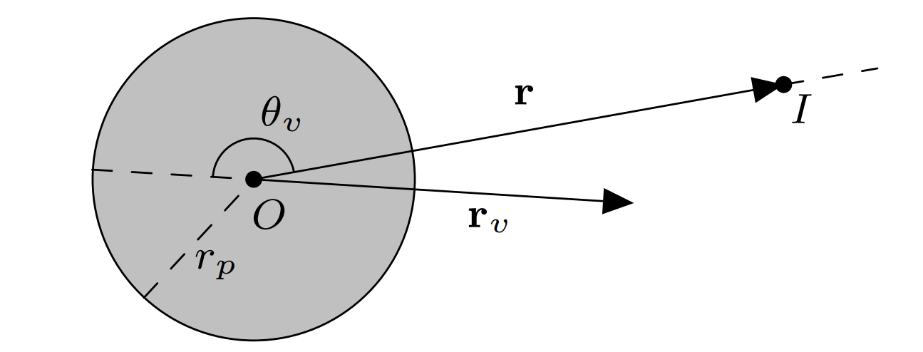

In this article, we relax assumptions from previous work (Jeannin et al. 2015; Jeannin et al. 2017) in order to give more maneuverability to the intruder. First, we do not necessarily assume that the horizontal rate of closure between the two aircraft is constant. Specifically, in the model in Section 5, we grant the intruder limited control over this value. This corresponds to the intruder being able to change direction in the horizontal plane during the encounter, represented in Fig. 3 by the angle between and .
Second, in the vertical direction, we not only allow the ownship’s vertical velocity to change at any moment, as in previous work, but we also grant the intruder limited control over its own vertical velocity (Sections 4, 7, and 9). In all encounters, we assume that the vertical acceleration of the intruder cannot exceed constant and that of the ownship cannot exceed . Any aircraft will have a rate of vertical acceleration which it cannot exceed due to the physical maneuverability limitations of the aircraft, and it is reasonable to assume for the ownship to have access to this value given the aircraft type of the intruder.
While these assumptions still limit the possible trajectories of each aircraft about which we will prove safety properties, they are necessary in the modeling and verification process. For instance, while it would be excellent to prove that the ownship can strategically wiggle out of a collision with any aircraft, this is just not possible if the intruder aircraft is strictly more maneuverable than the ownship. Thus, the constant is necessary to prove meaningful safety properties, even if it limits the types of encounters to which these safety properties apply.
2.2. Advisories
ACAS X advisories (except for the Clear-of-Conflict and Multi-Threat Level-Off advisories) have two components: a target velocity and the direction of the target . For example, the advisory CL1500 specifies that the pilot should achieve a climb rate of at least ft/min, meaning the target velocity is and the direction is upwards () allowing larger climb rates. For the DNC2000 advisory, the pilot is advised not to climb more than ft/min. This would make and . The and values of the ACAS X advisories are in Table 1.
2.3. Model Overview
We present a high-level model whose basic structure other models in this article follow.
| (1) | ||||
This dGL formula (1) of the shape says that there is a winning strategy for the ownship in the hybrid game starting in any state satisfying logical formula to end up in a state satisfying . The preconditions ensure both nature-imposed and safety-imposed conditions. Puck radii and must be positive, for instance, as they represent distances, since it flags an advisory as either upsense or downsense, and we need relationships between minimum advisory compliant climb rate , ownship climb rate limits , and intruder climb rate limits . We also that the ownship is initially in a safe region for some initial advisory , otherwise we cannot conclude that it will be safe in the future. This is symbolically represented above by the formula , but this region is both specific to the model being studied and critical to proving safety, and will therefore be developed and explained in great detail in each section.
The game on lines 1–1 encodes the sequence of discrete choices made, followed by the evolution of the continuous dynamics on line 1. Specifically, an advisory is computed () and issued on line 1 which must satisfy our safe region , after which the ownship is allowed in line 1 to choose the particular acceleration within the climb rate limits of the aircraft () that it wants to follow during the encounter. This choice of can access the advisory from line 1, but not the specific intruder choice from line 1 after it. Note that an important switch in coordinates over Table 1 occurs with respect to . Table 1 uses to refer to the climb rate requested from the ownship pilot, while in all our models refers to an advisory in terms of relative climb rate; the coordinate transformation to the non-relative advisory is assumed to occur in from relative and intruder velocity at the time of issuing the advisory. Then on line 1, the intruder can change its own control decision within climb rate limits , which we assume in init to be strict enough so that the ownship can overcome the worst-case intruder maneuvers given its own bounds . The differential equations of motion combine ownship and intruder acceleration to affect the relative climb rate , and in turn the vertical separation , while the horizontal separation is affected by the relative horizontal speed . The differential equations are followed for any duration of time, as long as the evolution domain constraint () is true. The evolution domain constraints vary depending on the model and will be discussed in later sections. The ∗ operator on line 1 indicates that the inner loop from line 1 to line 1 can be repeated any number of times so that the intruder can change decisions more often than the ownship. The bold-face intruder choice on line 1 and the inner loop operator on line 1 are omitted from models that do not allow the intruder control over its trajectory.
Crucially, the ownship choice on line 1 is contained within the operator, which represents the difference in choice between two players so between the ownship and intruder. The dGL formula states that given preconditions , there is a winning strategy for the ownship that wins by successfully achieving for all intruder responses when playing game . All choices within the game are resolved by our helpful player, so we need only show that there exists some run of this subgame such that for all runs of the game outside the operator, is satisfied. Within the context of this model, this means that there need only be one choice of which ultimately allows the ownship to avoid collision. Crucially, we will prove that for any advisory which satisfies our safe region and for any set of intruder actions, the pilot can strategically pick her acceleration such that an NMAC does not occur. By contrast, if this choice of were outside the operator, the model would be conjecturing that all of the infinitely many choices for ownship acceleration would have to satisfy the postcondition, which it simply does not if the pilot does not pay attention.
The last ∗ operator in line 1 is the outer loop around the entire program, which means that the aircraft encounter game can be repeated any number of times. More specifically, the pilot can be given any number of advisories by the aircraft, and our postcondition guarantees that any sequence of advisories which satisfy our safe region will guarantees collision freedom at all points in time.
2.4. Formalization and Verification Overview
The models and theorems in the following sections build upon the general shape (1) in an incremental fashion. An overview of the relationship between the models, definitions of safe regions, and safety theorems is given in Fig. 4.
3. Infinite-Time Safety for a Non-Maneuvering Intruder
In this section, we establish a baseline model in which the ownship and intruder are approaching each other at a constant horizontal velocity . In future sections, the intruder will have control over its vertical acceleration or the horizontal rate of closure to present a greater challenge to collision avoidance, but for now, the model is kept simple to establish a baseline understanding.
In this section, we define an advisory to be safe only if it is safe indefinitely, meaning that no further advisory is needed to provide long-term safety of the ownship. This is too restrictive for reasons discussed in Section 6, but it allows for a simple model with which to start our investigation.
3.1. Model
| init | |||
| R | |||
| advisory | |||
| ownship | |||
| motion | |||
The formula on line 1 is the safe region of this model: an ownship originally separated from an intruder by horizontally and vertically will avoid collision given the advisory . This crucial region will be developed and explained in Section 3.2. The postcondition on line 1 expresses the desire that there must always be a separation of the puck distance between the two aircraft in either the horizontal or vertical direction, so no NMAC ever occurs.
Lines 1–1 encode the advisory. The nondeterministic operator encodes that the pilot has two options: either to continue with her current advisory, in which case only the condition must be satisfied, or follow a new advisory. The operator discards any runs of the system in which the condition after the is false, so is always trivially satisfied. However, this condition is important to ensure that the system always has a valid choice for an advisory (i.e. keep the previous advisory), and will not get stuck without any safe advisories.
The requirement on line 1 is that the choice of target velocity and up or down advisory will keep the ownship within the safe region indefinitely, as encoded by the condition, given the minimum acceleration from Section 1.1. Without this assumption of a minimum acceleration, there is no guarantee in how quickly an aircraft would reach its target velocity, and therefore no safety guarantees.
Line 1 expresses the pilot’s choice of her own vertical acceleration . While this choice at first seems arbitrary in the context of the model, the proof will need to make strategic choices for within the climb rate limits of the aircraft to pass the subsequent test and avoid NMACs. Crucially, the choice of and test in line 1 are within a operator since the choice of and the responsibility of staying within the climb rate limits of the ownship are up to the ownship pilot.
The two aircraft then follow the differential equations on line 1. The differential equations express that , , and of the ownship evolve according to , the rate of horizontal closure, as well as the acceleration chosen by the pilot based on the advisory issued by the system.
3.2. Implicit Formulation of the Safe Region
As previously stated, the safety of this model hinges on proving that an aircraft following an advisory from line 1 will stay within the safe region throughout the encounter with an intruder. This begs the question of what regions of flight guarantee safety for the ownship. Just like the previous work, we represent this region with the formula . This region is fixed at the intruder with its origin at the initial position of the ownship. We will explain one case in detail and provide a generalization of this region after.
First case:
Consider the case of an upsense advisory , where the ownship has not yet reached the target velocity . We use the concept of a nominal trajectory (Jeannin et al. 2017) (denoted by ), an example of which is shown in Fig. 2 in red. In this figure, the ownship follows one possible trajectory adhering to all the requirements of ACAS X. This is just one of the uncountably infinitely many safe trajectories of the ownship. Upon receiving an advisory from ACAS X, the ownship begins climbing at an acceleration of and continues climbing along a parabola until it reaches the advised velocity . It then stops climbing and continues at the vertical velocity in a straight line. Through integration of the equations of motion from Model 1 line 1, we can get the coordinates of the ownship along this nominal trajectory as a function of time:
While these equations describe the minimally-compliant nominal trajectory, the ownship pilot’s choice of in line 1 can be different than (and may exceed it while necessary). The actual coordinates of the ownship could be anywhere above this safe nominal trajectory, creating a region in which the ownship is guaranteed to be. Thus, the ownship is safe if it is separated horizontally from the nominal trajectory by at least the puck width , or it is above the nominal trajectory by at least puck height , that is:
This will be referred to as the implicit formulation of the safe region. It is an implicitly defined region because it uses quantifiers as opposed to explicit inequalities to define the nominal trajectory.
Generalization:
The same reasoning applies to the case where the pilot is told to descend to avoid collision as well as the case, where the ownship has already achieved the target velocity and is now following the straight-line trajectory.
Going back to Model 1, the test on line 1 guarantees that following the nominal trajectory keeps the ownship safe, and thus we know that if the pilot accelerates at least as fast as the minimum acceleration or has already reached the target velocity, then she is above the nominal trajectory and is therefore safe as well. The test also allows the ACAS X system the flexibility to give any advisory which results in a safe nominal trajectory, and the pilot the flexibility to choose arbitrary accelerations which keep the plane in the implicit region. This safe region is used to prove the safety postcondition of Model 1, making it sufficient to reason about this region to guarantee the safety of the ownship. The implicit formulation follows (Jeannin et al. 2017, Fig. 3), is listed in Def. 3.1, and used in Theorem 3.2, which has been verified using KeYmaera X.
Definition 3.1 (Implicit Infinite-Time Safe Region).
Theorem 3.2 (Non-maneuvering intruder: correctness of implicit safe regions).
Proof.
The KeYmaera X proof develops a winning strategy for choosing ownship control :
We use minimal vertical acceleration in direction to adjust the climb rate towards the advisory. When the advisory is met (when ), we keep the climb rate steady by picking . ∎
4. Infinite-Time Safety for a Vertically-Maneuvering Intruder
Now that we have established a baseline model for this encounter which includes the important duality operator for player selection in hybrid games, we can continue on to more expressive models. Our next model accounts for vertical intruder maneuvers, and the model expresses the notion that the ownship should always have a way to overcome any reasonable intruder action. In the example shown in Fig. 5, even though the intruder begins accelerating in the same direction as the pilot, the pilot can still overcome the intruder action and navigate to safety.

4.1. Model
| init | |||
| R | |||
| advisory | |||
| ownship | |||
| intruder | |||
| motion | |||
In this section, the setup is very similar to the last. The intruder and ownship still approach one another with a constant horizontal rate of closure , and we have the same relative coordinate system with for relative horizontal distance between the aircraft and for relative vertical distance.
The difference in this model, highlighted in bold, is that we add the variable representing the intruder’s vertical acceleration, as well as a constant which represents the maximum magnitude of intruder acceleration, discussed previously in Section 2.1. On line 2, the intruder is now able to nondeterministically change its acceleration within and . The differential equations on line 2 have also been modified to incorporate the new dynamics of the intruder. The rate of vertical closure between the two aircraft now evolves at a rate of to reflect that both the intruder and ownship acceleration affect the rate of vertical closure. We choose to treat the rate of vertical closure as a relative rate as opposed to creating two separate absolute vertical velocities in order to minimize the number of variables needed in this model even if and are independent.
We add a loop around the intruder choice of acceleration and the dynamics on lines 2–2. The loop contains the intruder choice of acceleration, but not the ownship’s choice, meaning the intruder could change its acceleration any number of times during an interaction without the ownship being able to react. Recall that ACAS X tracks the position and velocity of the intruder, but not its acceleration (Office 2014a), so we cannot assume that the ownship has constant knowledge of the intruder’s acceleration. Therefore, the ownship must first make a choice in acceleration and stick with it while the intruder is more powerful and allowed to change its acceleration arbitrarily often.
This model comes with new strategic insights that are developed in the proof. The strategy chooses a relative rate of vertical separation (not the absolute ownship velocity) as the target velocity, or that the ownship is accelerating at least at the minimum velocity plus the maximum intruder acceleration as a strategy to overcome any possible intruder action. Since the ownship has access to the intruder’s velocity and position, it can reasonably monitor the rate of vertical separation. However, since the ownship does not have continuous access to intruder acceleration, it must choose an acceleration which can withstand changes to the intruder’s acceleration throughout the encounter. Therefore, if the ownship compensates by accelerating at least then the intruder will not be able to catch the ownship during the encounter, even in the worst cases of the intruder accelerating at or , because the relative acceleration difference will be at least .


Figure 6 shows an ownship following this new strategy from Theorem 4.1 with an intruder accelerating vertically at maximum climb rate , and Fig. 7 shows the ownship following the strategy from Theorem 3.2 with a non-maneuvering intruder. Note that the relative separation in the two figures evolves in the same way, since the ownship in Fig. 6 compensates the intruder maneuver by choosing a climb rate that accounts for the intruder maximum climb rate .
4.2. Implicit Formulation of the Safe Region
Despite the new collision avoidance strategy, we do not need to make any changes to the implicit safe region formulation. This is because the intruder dynamics are hidden by the variables and which represent relative vertical separation and rate of vertical closure. When the ownship strategically accelerates upwards with at least acceleration until reaching a vertical rate of separation of at least , since the intruder cannot accelerate more than , the relative rate of vertical acceleration is still at least . Therefore, our previous safe region from Def. 3.1 still applies with the coordinate system still fixed at the intruder.
Theorem 4.1 (Vertically maneuvering intruder: Correctness of implicit safe regions).
Proof.
The KeYmaera X proof develops a winning strategy for choosing ownship control :
We compensate intruder maneuvers with increased minimal vertical acceleration in direction to adjust the climb rate towards the advisory. When the ownship follows the issued advisory (when ), we pick to compensate intruder maneuvers and maintain following the advisory. The safe region serves as a loop invariant of the outer loop of Model 2. Since the ownship control choice in the winning strategy is only safe when the ownship already follows the issued advisory, in this case we additionally show that following the advisory () is an invariant of the inner loop. ∎
5. Infinite-Time Safety for a Horizontally-Maneuvering Intruder
Where Model 2 expands on Model 1 by granting the intruder limited control over its vertical velocity, Model 3 in this section grants the intruder limited control over the horizontal rate of closure. The intruder can increase its ground velocity towards the ownship, as well as change the angle shown in Fig. 3 in order to alter the rate of closure between the two aircraft.
5.1. Model
| init | |||
| R | |||
| advisory | |||
| ownship | |||
| intruder | |||
| motion | |||
In Model 3, we give control of the horizontal rate of closure to the intruder. We do not assume horizontal maneuverability for the ownship, but the intruder has sole control over the horizontal rate of closure, and can therefore nondeterministically choose on line 3. This requires the new safe region on line 3. Just as in the previous section, we must assume some upper limit on the intruder maneuverability; therefore, we introduce the constant on line 3 to represent the maximum possible horizontal rate of closure between the two aircraft. For simplicity, we also assume that the intruder’s maneuvers cannot invert the rate of closure, meaning the intruder cannot fully turn around during the encounter , and must be non-negative. This assumption ensures that the intruder is not fully adversarial and will not ascend or descend along a helix, or turn around to chase the ownship.
Besides these changes, the dynamics mirror that of Model 1. Again, the loop around the intruder choice and the dynamics allows the intruder to change the rate of closure as many times as it pleases during the encounter, but the ownship must stick with its initial choice of acceleration.
5.2. Implicit Formulation of the Safe Region
The safe region of this model must take into consideration the variable rate of closure , which could vary anywhere from to . As such, we no longer have a single nominal trajectory, but infinitely many nominal trajectories which are a function of the horizontal rate of closure chosen by the intruder. Each nominal trajectory is the same as in Sections 3 and 4:
However, in order for our region to be safe, we must know that each nominal trajectory whose is within keeps a safe distance from the intruder at all future points in time. This motivates universally quantifying over all possible choices of in our new region:
If this region holds for some advisory , we know that for any possible horizontal rate of closure chosen by the intruder, if the ownship obeys the advisory then it will avoid an NMAC. The implicit formulation is shown in Def. 5.1 and used in Theorem 5.2, which has been verified to be safe using KeYmaera X.
Definition 5.1 (Lower-bounded, infinite time safe region with horizontally-maneuvering intruder).
with and as per Def. 3.1.
Theorem 5.2 (Horizontally-maneuvering intruder: correctness of implicit safe regions).
Proof.
The KeYmaera X proof develops a winning strategy for choosing ownship control :
We use minimal vertical acceleration in direction to adjust the climb rate towards the advisory. When the advisory is met (when ), we keep the climb rate steady by picking . ∎
6. Bounded-Time Safety for a Non-Maneuvering Intruder
Up to this point, the models described in this article have all conveyed the notion that advisories issued by the ACAS X system must be safe indefinitely; that is, while the system can issue new advisories at any point, the aircraft must avoid collision whether or not the system issues a new advisory to pass our rigorous notion of safety. In the context of the above models, this need comes from the lack of a time bound on the differential equations, so every duration of the differential equation must guarantee safety for our model to be safe, even without another advisory change.
In a realistic scenario, this idea is limiting because it typically forces the system to give fairly strong advisories too early on and too frequently. While this is acceptable from a safety-perspective, it is unacceptable from a pilot-perspective. A system which gives overly frequent advisories can be distracting to the pilot and may lead the pilot to ignore the system warnings all together. Thus, if an encounter is not immediately threatening, the ACAS X implementation will actually issue COC or a preventative advisory like DNC or DND, and will later issue a more disruptive advisory as the threat level increases. In cases like this, the preliminary advisory may not be safe indefinitely, but safety can later be restored with a subsequent advisory (as will be the case in Fig. 10).
We represent this idea through the concept of safeability from previous ACAS X work (Jeannin et al. 2017).
Definition 6.1 (Safeable).
We say that an advisory is safeable if and only if it is safe or can still be made safe in the future, if necessary, via subsequent advisories.
In other words, we need only ensure the safety of an advisory for a few seconds as long as some followup advisory exists that will keep us safe forever. Once again, the safeable region of a given advisory is always a superset of its safe region, so safeability is a more robust definition.
To develop the safeability models, we assume that the ownship and intruder are approaching at a constant horizontal rate of closure , and and represent the relative horizontal and vertical separation, respectively. A subsequent advisory is called a reversal when the sign of reverses from the initial advisory. If does not change, the subsequent advisory is a strengthening or weakening.

Given the complexity of proving safeability, we first prove bounded-time, upper and lower bounded safe regions as building blocks to proving safeability. All previous safe regions constructed in this article have only been lower-bounded for (or only upper-bounded for ), meaning the ownship must achieve some minimum acceleration or velocity in order to stay within the region. We now incorporate two-sided bounds on the ownship’s acceleration and vertical velocity to construct a region which is bounded from above and below (see Fig. 8). This is important because in a safeable scenario, the ownship could receive a reversal advisory, meaning it must reverse its direction of flight between the first and second advisories. In this case, it is imperative that we know both an upper and lower bound on the trajectory of the ownship in the first phase of flight in order to reason about its position and velocity in the second phase of flight.
The following models prove safety of the two-sided safe regions only up to some time . While it is not sufficient only to prove safety for some bounded amount of time, this step lays important groundwork for proving the fully safeable region in Section 8. The safeable proofs require that an advisory be provably safe only for time and that some followup advisory is safe indefinitely, so the bounded-time proof is a necessary stepping stone to ultimately proving the safeable region.
We, again, start with the model which allows no maneuverability to the intruder before moving on to the model which allows the intruder to accelerate vertically.
6.1. Model
| init | |||
| R | |||
| advisory | |||
| ownship | |||
| motion | |||
First, we add symbolic upper bounds on the ownship acceleration and vertical velocity (usually and ft/min, respectively). The upper bound increases the complexity of the ownship strategy: the strategy in Theorem 3.2 picked acceleration towards satisfying , but now we must ultimately adjust this choice again before violating . We address this with an event-triggered design in lines 4–4 with evolution domain constraints to monitor when crosses . In order to not discard behavior for the sake of detecting this event, we follow the standard pattern (Quesel et al. 2016) to model event monitoring with overlapping evolution domain constraints.22 2 The notation is shorthand notation for the non-deterministic choice between ODEs that only differ in their evolution domain constraints: . Crucially, differs from in its ability to detect the events of handover from to or vice versa. We get notified that an event occurred exactly at the boundary where the two evolution domain constraints and overlap. Through the loop on lines 4–4, the ownship can react to the event by selecting a new acceleration in line 4.
To model the bounded-time safety, we add variable which acts as a timer for the duration of the dynamics. It is reset to on line 4 at the beginning of each new advisory and evolves at a constant rate in the dynamics equation on line 4. Once this variable reaches , the differential equations are stopped from evolving further, and a new advisory must be issued. This time bound guarantees that the ownship will be given a new advisory and update its acceleration after at most -time has passed. The time-unbounded case is represented with the condition .
Another important difference introduced in this model is the removal of the test from line 4. This has been removed to disallow the ownship from blindly continuing with the old advisory after time. While the same advisory can be given on each iteration of the loop, the removal of the test ensures that new advisories will definitely be considered after each time step.
Even though a new advisory is given after time elapses, this does not mean that a safe advisory exists. If no safe advisory exists, the test on line 4 would fail, and the model would be vacuously true since no possible runs of the system exist (and therefore all runs satisfy the postcondition). Thus, our model is only meaningful for time, after which we cannot draw any meaningful conclusions about safety. However, we address this issue of liveness in the models in Sections 8 and 9.
6.2. Implicit Formulation of the Safe Region
The safe region of this model now consists of two separate safe regions, the lower bounded region , and the new upper region listed in Def. 6.2.
The following observation is important for understanding the safe regions. In the event that the ownship is already exceeding when receiving the advisory, it is unrealistic for the pilot to accelerate downwards to reach the upper bound from above. Instead, we assume the pilot will not accelerate further if she has already exceeded the target . Therefore, on an initial overcompliance in vertical velocity , the target velocity becomes as opposed to .
First case:
Consider and . Just like for the lower safe region, we consider a nominal trajectory to characterize the upper safe region. In this region, we again accelerate upwards at the upper acceleration until reaching (or in the case of initial overcompliance) and then continue linearly at velocity max. As before, we continue at a constant horizontal velocity . We give the position along the nominal trajectory as a function of time:
In the same way that we knew that the ownship is above the nominal trajectory in the lower-bounded region, we know that the ownship will be below this upper nominal trajectory because and (or ). Therefore, in order to ensure safety of the ownship we need:
Now that we have the regions and (Def. 6.2), we can characterize the two-sided safe region as their disjunction. Given the fact that , we know that the ownship stays between the two nominal trajectories, so its flight is properly upper and lower bounded; thus, as long as either the lower nominal trajectory or the upper nominal trajectory avoids collision, the ownship will be safe. This is the motivation for the disjunction of the two safe regions: since the ownship is between the two trajectories, only one trajectory needs to be safe for the ownship to be safe as well. The implicit formulation of is shown in Def. 6.2 and used in Theorem 6.3, which has been verified to be safe using KeYmaera X.
Definition 6.2 (Implicit formulation of the two-sided safe region).
with and per Def. 3.1.
Theorem 6.3 (Bounded-time non-maneuvering intruder: correctness of two-sided bounded-time safe regions).
Proof.
The KeYmaera X proof develops a winning strategy for choosing ownship control :
We pick to accelerate towards the advisory if the ownship is not yet in compliance . This case crucially relies on the event-triggered design, which notifies the ownship of a required change in strategy before violating . When in compliance or in overcompliance , we simply pick to maintain the current climb rate. The safe region serves as a loop invariant. ∎
7. Bounded-Time Safety for a Vertically-Maneuvering Intruder
With the groundwork laid in Section 6, we expand Model 4 for bounded-time safety to Model 5 where we allow the intruder to control its vertical velocity.
7.1. Model
| init | |||
| R | |||
| advisory | |||
| estimate | |||
| ownship | |||
| intruder | |||
| motion | |||
Again, the variables and as well as the constants and represent the upper safe region and our time bound, the variable tracks the intruder’s acceleration, and we allow it to affect the relative vertical velocity . The main update in Model 5 is how the ownship reacts to intruder behavior. In line 5, the ownship estimates a bound for the upcoming intruder acceleration (e.g., the worst-case bound or a less permissive bound). The ownship strategy can take this estimate into account when picking acceleration . The intruder then, in line 5, gets to select intruder acceleration : if that choice happens to fit to the ownship estimate, the test passes and the model continues with motion on lines 5–5. Otherwise the test fails and the only runs either have the intruder change its acceleration choice through the loop in lines 5–5, or have control return to the ownship via the loop on lines 5–5 to update the estimate . This model allows for a variety of system implementations over a range of interaction requirements:
- •
no interaction between intruder and ownship is required when the ownship uses the worst-case acceleration as its estimate ;
- •
the ownship may detect when the intruder acceleration exceeds the estimate and change its strategy in return;
- •
the ownship and intruder may cooperate to pick the bound ;
- •
the ownship may announce the bound as a requirement to the intruder.
The evolution domain constraint is again modified to detect when the relative climb rate falls below or exceeds the target , so that the ownship can change its strategy for overcoming the intruder motion. The event detection mechanism of Model 4 is extended in line 5 to detect when the ownship is about to no longer satisfy , and so includes the choice between overlapping evolution domain constraints .
Figure 9 shows an example comparison of the current and former safe regions given the new intruder maneuverability. For simplicity we explain only the strategy for the upsense case and the worst-case intruder acceleration . In order to continue evolving, just as in the infinite-time Model 2 from Section 4 the ownship acceleration must be at least , or the ownship velocity is at least . Simultaneously, the ownship either initially overcomplies in terms of velocity (), or its velocity must not exceed and its acceleration must not exceed . In this first case of overcompliance, it is no longer enough to stop accelerating upwards. The ownship now needs to compensate for the fact that the intruder could be accelerating downwards with acceleration at most by accelerating downwards with acceleration as well.

7.2. Implicit Formulation of the Safe Region
The safe region of this model is exactly the same as that from Section 6. Due to the full relativization of both the rate of vertical closure and vertical separation, as well as the requirement that , the with coordinate system fixed at the intruder still applies to this model.
Theorem 7.1 (Bounded-time vertically-maneuvering intruder: correctness of two-sided bounded-time safe regions).
Proof.
The KeYmaera X proof develops a winning strategy for choosing ownship control in reaction to the worst-case intruder acceleration estimate :
If the ownship is not yet in compliance , We pick , which is the minimum compliant acceleration compensated for worst-case intruder acceleration . When in compliance , we pick for proof simplicity, but any acceleration that does not exceed the upper acceleration compensated for worst-case intruder acceleration would work as well. Finally, in overcompliance , we decelerate downwards with to compensate for worst-case intruder acceleration . ∎
Unlike in the non-maneuvering case Theorem 6.3, in the presence of a vertically maneuvering intruder there exists no choice of that keeps the relative climb rate constant, since the intruder is allowed to change its acceleration arbitrarily often. As a result, in Theorem 7.1 the choice of , and any other choice in , crucially relies on the event detection that informs the ownship when is about to be violated and a change in strategy is required.
8. Safeability for a Non-Maneuvering Intruder
In this section, we combine bounded-time safety with infinite-time safety to the notion of safeability: it is safe to follow a bounded-time region if there exists an infinite-time follow-up advisory. The intuition behind the safeable region is shown in Fig. 10.

We consider all the possible positions and speeds that the ownship could end up after time, in particular the lowest and highest such speeds and positions. At the lowest position, the most extreme strengthening is most critical, and at the highest position the most extreme reversal is most critical. The two safe regions achieved by these strengthenings and reversals give us the regions of ownship position which we can achieve by acting at time . This is precisely the safeable region: the safe region achieved by following a weaker advisory until time and then following a stronger advisory indefinitely.
8.1. Model
| init | |||
| R | |||
| advisory | |||
| ownship | |||
| motion | |||
8.2. Implicit Formulation of the Safe Region
The region again consists of a lower bound and an upper bound: regions and now combine two separate conditions: a region up to time and a region from time onward. Up to time , we follow bounded-time and from Def. 6.2. In order to be allowed to issue an advisory, the region now encodes that from time onward there must exist a new advisory given the potential ownship velocity and vertical separation at time under which the infinite regions and are satisfied.
Note that this model is similar to the previous bounded-time Model 4 but also proves liveness: after the time bound, we guarantee the existence of another advisory which keeps the ownship safe. The final region is a disjunction of and .
Theorem 8.2.
Proof.
The KeYmaera X proof develops a winning strategy for choosing ownship control :
The proof is more involved, because the theorem is stronger, but the strategy is as in the bounded-time case. We pick to accelerate towards the advisory if the ownship is not yet in compliance . We can keep this strategy until the event-trigger that the ownship has reached the advisory . When , we pick so that stays within and . The ownship can choose an advisory that does not keep it within this range indefinitely, but it then relies on the event-trigger to notify when it is no longer in compliance, necessitating a new choice of acceleration. In the overcompliance case, we again choose for . The safe region serves as a loop invariant. Due to this invariant, we know the existence of a future advisory such that the ownship will be safe indefinitely after using these strategies for the initial time. ∎
9. Safeability for a Vertically-Maneuvering Intruder
Taking all of the groundwork laid by the previous sections, we finally present the model and safeable regions generalized for the case where the intruder can change its vertical acceleration.
9.1. Model
| init | |||
| R | |||
| advisory | |||
| estimate | |||
| ownship | |||
| intruder | |||
| motion | |||
Again, we represent the intruder choice for at line 7 and the bound on this choice, as well as the loop around the intruder choice and dynamics to reflect that the intruder can change its acceleration throughout the encounter without the ownship being alerted to these changes.
The safe region for Model 7 follows Def. 8.1 due to the relativization of the vertical rate of closure and vertical separation.
Theorem 9.1.
Proof.
The KeYmaera X proof develops a winning strategy for choosing ownship control in reaction to the worst-case intruder acceleration estimate :
This strategy matches that of the bounded time case. Again, if the ownship is not yet in compliance , we pick . When the ownship is compliant, with , we pick , and in the overcompliance case, we accelerate downwards with . With the safe region as the loop invariant, we know that a future advisory exists which will keep the ownship safe indefinitely, assuming the ownship follows these strategies up to time. ∎
10. Discussion
Each of the proofs of the theorems presented in this article were completed in KeYmaera X with support of Mathematica’s implementation of real quantifier elimination (Collins 1976). Besides designing the hybrid game model and identifying the safe regions for its advisories, the main insights in the proofs are the invariants and winning strategies. The verified models crucially extends previous work with a rich representation of intruder behavior and its potentially adversarial nature. The benefit of attributing different actions to different players in the game is that we can now represent interactions between the ownship and the intruder, including worst-case non-cooperative interactions, as well as interactions in which the intruder and ownship react to one another.
Hybrid games verification, however, leads to even more complicated real arithmetic decision problems, which, even if decidable, may need time-consuming, handmade proof simplification for the proof to close. The arithmetic complexity of the safe regions required an intimate knowledge in order to simplify the proof into pieces digestible to Mathematica. This was particularly relevant compared to hybrid systems ACAS X verification (Jeannin et al. 2017) due to the addition of quantifier alternation stemming from games and new variables and constants to represent the intruder’s maneuverability, as well as the introduction of more relationships between these values in the preconditions. The majority of manual arithmetic simplifications are case splitting (e.g., between or ), providing witnesses to quantifiers according to the winning strategy to help solvers, abbreviating terms to make inequality transitivity obvious, and selecting the relevant assumptions from the list of all assumptions. Table 2 compares our proofs in terms of tactic size as an indicator for relative manual proof effort, and proof checking duration as an indicator of arithmetic complexity.
| Model | Intruder | Tactic steps | Proof checking [s] | ||||
|---|---|---|---|---|---|---|---|
| Vert. | Horiz. | Total | QE | RCF | |||
| Infinite | Model 1, Theorem 3.2 | 163 | 18 | 15 | 12 | ||
| Model 2, Theorem 4.1 | 196 | 35 | 30 | 26 | |||
| Model 3, Theorem 5.2 | 242 | 35 | 29 | 23 | |||
| Bounded | Model 4, Theorem 6.3 | 540 | 112 | 97 | 79 | ||
| Model 5, Theorem 7.1 | 724 | 319 | 298 | 177 | |||
| Safeable | Model 6, Theorem 8.2 | 3402 | 1786 | 886 | 279 | ||
| Model 7, Theorem 9.1 | 2782 | 1404 | 1163 | 247 | |||
Its content has to be taken with a grain of salt, because there is considerable freedom in designing proofs and in making the tradeoff between manual steps and duration of arithmetic proof obligations. We observe a few general trends across models:
- •
Even with manual simplification, the real arithmetic proof obligations are responsible for a considerable portion of the proof-checking duration;
- •
Infinite-time models are considerably easier (smaller tactic size, faster proof) than bounded-time models, which are in turn considerably easier than safeable models;
- •
Intruder maneuverability increases proof complexity, but experience from controlling the branching when proving the many ways of ownship and intruder interaction in the non-maneuvering safeable model helped finding a smaller tactic design and faster proof in the vertical safeable model;
- •
The large number of combinations of ownship and intruder interactions in the safeable models makes it infeasible to manually simplify all the arithmetic proof obligations, which results in considerably longer proof checking duration; the large difference in the proofs of Model 6 and Model 7 between the duration of all proof attempts in the tactic QE and the duration of its successful attempt in column RCF indicates a potential for improving tactic heuristics or parallelization.
The increased complexity that each new variable introduces motivated our decision to relativize the rates of closure. This simplified the model and arithmetic, and allowed for the same region from the corresponding non-maneuvering intruder to be used. We cannot further relativize the models beyond the rates of closure, however; it is important that each actor in the encounter have sole control over their own accelerations independently to properly model that both actors can affect the outcome of an encounter in this aircraft game scenario.
In terms of proof construction, the main challenge was in the development of the winning strategies for the ownship. This is a particular challenge in proving hybrid games; the ownship must pick a strategy without any knowledge of what the intruder may end up choosing, only knowledge of the broad limitations of the intruder’s maneuvering capabilities. In the context of ACAS X, this is complicated by the fact that the ownship does not have access to the acceleration of the intruder, so it cannot react to the intruder’s choice of acceleration to update its own choice. Therefore, it was imperative to have a proper strategy in choosing the pilot’s acceleration in order to prove our intruder-maneuverability models.
A final challenge in hybrid game modeling is in the correct assignment of player responsibility for a given action. It is vital to the fidelity of the model that the choices in the model be resolved by the correct player to prevent one player having an unfair advantage. For instance, if the choice of advisory were resolved by the ownship, the ownship could choose an optimal advisory to follow. However, the choice of advisory needs to be resolved by the intruder because that proves that all of the advisories which satisfy the safe region can be chosen and are shown safe.
11. Related Work
Kochenderfer and Chryssanthacopoulos (Kochenderfer et al. 2008) design the ACAS X lookup tables, the verification of which motivates this work (see Section 1.1). Von Essen and Giannakopoulou (von Essen and Giannakopoulou 2014) use probabilistic model-checking in their analysis of a similar Markov Decision Process (Kochenderfer et al. 2008), to explore the probability of occurrence of various unfavorable events. The outcome is limited due to its discretization of the continuous dynamics in analyzing the system and the implausible assumption that the intruder follows a random walk in the decision space.
Holland et al. (Holland et al. 2013) and Chludzinski (Chludzinski 2009) simulate encounters, many of which come from recorded flight data. Lee, et al. (Lee et al. 2018) develops a technique called differential adaptive stress testing to find scenarios in which TCAS does not result in an NMAC, but ACAS X does. These simulations provide interesting evaluations of the performance of ACAS X, but only explore a finite set of the state space and therefore cannot allow any conclusions about the infinitely many other possible behaviors.
Julian and Kochenderfer (Julian et al. 2018) train a deep neural network to approximate the ACAS X lookup table to reduce the storage needs and runtime of the system, and Irfan, et al. (Irfan et al. 2020) and Julian and Kochenderfer (Julian and Kochenderfer 2021) explore applying formal methods to verify such neural networks. One drawback to this approach is that SMT does not support continuous dynamics, and all queries to the SMT solver must be in the form of discrete, linear regions. The inherent nonlinearity of the relevant regions when verifying ACAS X severely limits the verifying ability of this approach.
Kouskoulas, et al. (Kouskoulas et al. 2017) develop a formally verified, quantifier-free predicate which, given a sequence of timed ownship and intruder maneuvers, checks whether or not an NMAC may occur. They do so by establishing envelopes around either aircraft that contain all altitudes reachable by each aircraft through each maneuver. While this work verifies the safety of pre-determined encounters between an ownship and intruder accelerating non-deterministically, it requires knowledge of the full sequence of maneuvers which the intruder will perform beforehand. Our work instead proves safety assuming no knowledge of the sequence of intruder maneuvers, better capturing the uncertain adversarial abilities of the intruder.
Lygeros and Lynch (Lygeros and Lynch 1997) explore verification of the conflict resolution algorithms used in TCAS, a predecessor of ACAS X, with hybrid techniques. This work is limited in its overzealous use of assumptions, for instance in assuming that two aircraft both using TCAS will ultimately be given opposite advisories in an encounter. Our work does not make assumptions about the actions of the intruder and ownship relative to one another; the decisions of one aircraft are independent from those of the other as are best expressed with game models.
Tomlin et al. (Tomlin et al. 1998) presents a methodology with which to develop safe collision-avoidance maneuvers using hybrid systems. Platzer and Clarke (Platzer and Clarke 2009), Loos et al. (Loos et al. 2013) and Ghorbal et al. (Ghorbal et al. 2014) also use hybrid systems to design and verify their own horizontal collision avoidance maneuvers. Dowek et al. (Dowek and Muñoz 2005) and Galdino et al. (Galdino et al. 2007) design their own algorithms for collision avoidance, known as KB3D and KB2D, respectively, and verify their geometry using the PVS theorem prover.
Other approaches for hybrid games have limited real-world applications due to the overly-restrictive assumptions that they place on the systems which they represent. Henzinger et al. (Henzinger et al. 1999) work with rectangular hybrid games, which require strict upper and lower bounds on the continuous dynamics of the system and forgetful transitions. This work is one of the first case studies for hybrid games verification, the only example that we are aware of coming from Quesel and Platzer (Quesel and Platzer 2012) in their feasibility study involving an abstract robot in a factory.
12. Conclusion and Future Work
We applied hybrid games to the verification of ACAS X to prove that under limited horizontal and vertical maneuverability of an adversarial intruder, an ownship given a safe advisory from ACAS X always has a strategy to find a trajectory which avoids an NMAC despite subsequent intruder maneuvering. This work employed the principle of our previous work (Jeannin et al. 2017) to identify regions of safety, whereby following any advisory in the safe region has an ownship strategy that will keep the aircraft clear of an NMAC. The safe regions and intruder capabilities are symbolic such that these models can be reused for future versions of ACAS X and apply to any intruder which is less maneuverable than the ownship. While increased arithmetic and proof complexity is the downside of working with hybrid games, the advantage is the significantly increased resulting predictive power, because collision freedom can be proved even if the intruder is maneuvering, which it will in reality. In future work, we plan to explore verifying more complex ownship maneuvers in the horizontal direction and apply horizontal intruder maneuverability to the safeable model.
Acknowledgements.
This research was sponsored by the Sponsor AFOSR under grant number Grant #FA9550-16-1-0288. The views and conclusions contained in this document are those of the authors and should not be interpreted as representing the official policies, either expressed or implied, of any sponsoring institution, the U.S. government or any other entity.References
- (1)
- Chludzinski (2009) Barbara J. Chludzinski. 2009. Evaluation of TCAS II version 7.1 using the FAA fast-time encounter generator model. Technical Report. MIT Lincoln Laboratory.
- Collins (1976) George E. Collins. 1976. Quantifier Elimination for Real Closed Fields by Cylindrical Algebraic Decomposition: a synopsis. SIGSAM Bull. 10, 1 (1976), 10–12. https://doi.org/10.1145/1093390.1093393
- Dowek and Muñoz (2005) Gilles Dowek and César Muñoz. 2005. Provably Safe Coordinated Strategy for Distributed Conflict Resolution. AIAA Guidance, Navigation, and Control Conference (08 2005). https://doi.org/10.2514/6.2005-6047
- Fulton et al. (2015) Nathan Fulton, Stefan Mitsch, Jan-David Quesel, Marcus Völp, and André Platzer. 2015. KeYmaera X: An Axiomatic Tactical Theorem Prover for Hybrid Systems. In Automated Deduction - CADE-25 - 25th International Conference on Automated Deduction, Berlin, Germany, August 1-7, 2015, Proceedings (LNCS, Vol. 9195), Amy P. Felty and Aart Middeldorp (Eds.). Springer, Cham, 527–538. https://doi.org/10.1007/978-3-319-21401-6_36
- Galdino et al. (2007) André Luiz Galdino, César A. Muñoz, and Mauricio Ayala-Rincón. 2007. Formal Verification of an Optimal Air Traffic Conflict Resolution and Recovery Algorithm. In Logic, Language, Information and Computation, 14th International Workshop, WoLLIC 2007, Rio de Janeiro, Brazil, July 2-5, 2007, Proceedings (LNCS, Vol. 4576), Daniel Leivant and Ruy J. G. B. de Queiroz (Eds.). Springer, Berlin, Heidelberg, 177–188. https://doi.org/10.1007/978-3-540-73445-1_13
- Ghorbal et al. (2014) Khalil Ghorbal, Jean-Baptiste Jeannin, Erik Zawadzki, André Platzer, Geoffrey J. Gordon, and Peter Capell. 2014. Hybrid Theorem Proving of Aerospace Systems: Applications and Challenges. J. Aerosp. Inf. Syst. 11, 10 (2014), 702–713. https://doi.org/10.2514/1.I010178
- Henzinger et al. (1999) Thomas A. Henzinger, Benjamin Horowitz, and Rupak Majumdar. 1999. Rectangular Hybrid Games. In CONCUR ’99: Concurrency Theory, 10th International Conference, Eindhoven, The Netherlands, August 24-27, 1999, Proceedings (LNCS, Vol. 1664), Jos C. M. Baeten and Sjouke Mauw (Eds.). Springer, 320–335. https://doi.org/10.1007/3-540-48320-9_23
- Holland et al. (2013) Jessica Holland, Mykel Kochenderfer, and Wesley Olson. 2013. Optimizing the Next Generation Collision Avoidance System for Safe, Suitable, and Acceptable Operational Performance. Proceedings of the 10th USA/Europe Air Traffic Management Research and Development Seminar, ATM 2013 21 (07 2013). https://doi.org/10.2514/atcq.21.3.275
- Irfan et al. (2020) Ahmed Irfan, Kyle D. Julian, Haoze Wu, Clark Barrett, Mykel J. Kochenderfer, Baoluo Meng, and James Lopez. 2020. Towards Verification of Neural Networks for Small Unmanned Aircraft Collision Avoidance. In 2020 AIAA/IEEE 39th Digital Avionics Systems Conference (DASC). 1–10. https://doi.org/10.1109/DASC50938.2020.9256616
- Jeannin et al. (2015) Jean-Baptiste Jeannin, Khalil Ghorbal, Yanni Kouskoulas, Ryan W. Gardner, Aurora Schmidt, Erik Zawadzki, and André Platzer. 2015. A Formally Verified Hybrid System for the Next-Generation Airborne Collision Avoidance System. In Tools and Algorithms for the Construction and Analysis of Systems - 21st International Conference, TACAS 2015, Held as Part of the European Joint Conferences on Theory and Practice of Software, ETAPS 2015, London, UK, April 11-18, 2015. Proceedings (LNCS, Vol. 9035), Christel Baier and Cesare Tinelli (Eds.). Springer, Berlin, Heidelberg, 21–36. https://doi.org/10.1007/978-3-662-46681-0_2
- Jeannin et al. (2017) Jean-Baptiste Jeannin, Khalil Ghorbal, Yanni Kouskoulas, Aurora Schmidt, Ryan W. Gardner, Stefan Mitsch, and André Platzer. 2017. A formally verified hybrid system for safe advisories in the next-generation airborne collision avoidance system. Int. J. Softw. Tools Technol. Transf. 19, 6 (2017), 717–741. https://doi.org/10.1007/s10009-016-0434-1
- Julian and Kochenderfer (2021) Kyle D. Julian and Mykel J. Kochenderfer. 2021. Reachability Analysis for Neural Network Aircraft Collision Avoidance Systems. Journal of Guidance, Control, and Dynamics 44, 6 (2021), 1132–1142. https://doi.org/10.2514/1.G005233 arXiv:https://doi.org/10.2514/1.G005233
- Julian et al. (2018) Kyle D. Julian, Mykel J. Kochenderfer, and Michael P. Owen. 2018. Deep Neural Network Compression for Aircraft Collision Avoidance Systems. CoRR abs/1810.04240 (2018), 598–608. arXiv:1810.04240 http://arxiv.org/abs/1810.04240
- Kochenderfer et al. (2012) Mykel Kochenderfer, Jessica Holland, and James Chryssanthacopoulos. 2012. Next generation airborne collision avoidance system. Lincoln Laboratory Journal 19 (01 2012), 17–33.
- Kochenderfer et al. (2008) Mykel J. Kochenderfer, L. P. Espindle, James K. Kuchar, and John Daniel Griffith. 2008. Correlated Encounter Model for Cooperative Aircraft in the National Airspace System Version 1.0.
- Kouskoulas et al. (2017) Yanni Kouskoulas, Daniel Genin, Aurora Schmidt, and Jean-Baptiste Jeannin. 2017. Formally Verified Safe Vertical Maneuvers for Non-deterministic, Accelerating Aircraft Dynamics. In Interactive Theorem Proving - 8th International Conference, ITP 2017, Brasília, Brazil, September 26-29, 2017, Proceedings (LNCS, Vol. 10499), Mauricio Ayala-Rincón and César A. Muñoz (Eds.). Springer, 336–353. https://doi.org/10.1007/978-3-319-66107-0_22
- Lee et al. (2018) Ritchie Lee, Ole Mengshoel, Anshu Saksena, Ryan Gardner, Daniel Genin, Jeffrey Brush, and Mykel J. Kochenderfer. 2018. Differential Adaptive Stress Testing of Airborne Collision Avoidance Systems. https://doi.org/10.2514/6.2018-1923 arXiv:https://arc.aiaa.org/doi/pdf/10.2514/6.2018-1923
- Loos et al. (2013) Sarah M. Loos, David W. Renshaw, and André Platzer. 2013. Formal verification of distributed aircraft controllers. In Proceedings of the 16th international conference on Hybrid systems: computation and control, HSCC 2013, April 8-11, 2013, Philadelphia, PA, USA, Calin Belta and Franjo Ivancic (Eds.). ACM, Philadelphia, PA, 125–130. https://doi.org/10.1145/2461328.2461350
- Lygeros and Lynch (1997) J. Lygeros and N. Lynch. 1997. On the formal verification of the TCAS conflict resolution algorithms. In Proceedings of the 36th IEEE Conference on Decision and Control, Vol. 2. 1829–1834 vol.2. https://doi.org/10.1109/CDC.1997.657846
- Office (2014a) Federal Aviation Administration TCAS Program Office. 2014a. Algorithm design description for the surveillance and tracking module of ACAS X, run12.
- Office (2014b) Federal Aviation Administration TCAS Program Office. 2014b. Algorithm design description for the threat resolution module of ACAS X, version 3 Rev. 1.
- Platzer (2008) André Platzer. 2008. Differential Dynamic Logic for Hybrid Systems. J. Autom. Reas. 41, 2 (2008), 143–189. https://doi.org/10.1007/s10817-008-9103-8
- Platzer (2010) André Platzer. 2010. Logical Analysis of Hybrid Systems: Proving Theorems for Complex Dynamics. Springer, Heidelberg. https://doi.org/10.1007/978-3-642-14509-4
- Platzer (2012) André Platzer. 2012. Logics of Dynamical Systems. In LICS. IEEE, 13–24. https://doi.org/10.1109/LICS.2012.13
- Platzer (2015) André Platzer. 2015. Differential Game Logic. ACM Trans. Comput. Log. 17, 1 (2015), 1:1–1:51. https://doi.org/10.1145/2817824
- Platzer (2017a) André Platzer. 2017a. A Complete Uniform Substitution Calculus for Differential Dynamic Logic. J. Autom. Reas. 59, 2 (2017), 219–265. https://doi.org/10.1007/s10817-016-9385-1
- Platzer (2017b) André Platzer. 2017b. Differential Hybrid Games. ACM Trans. Comput. Log. 18, 3 (2017), 19:1–19:44. https://doi.org/10.1145/3091123
- Platzer (2018) André Platzer. 2018. Logical Foundations of Cyber-Physical Systems. Springer, Cham. https://doi.org/10.1007/978-3-319-63588-0
- Platzer and Clarke (2009) André Platzer and Edmund M. Clarke. 2009. Formal Verification of Curved Flight Collision Avoidance Maneuvers: A Case Study. In FM (LNCS, Vol. 5850), Ana Cavalcanti and Dennis Dams (Eds.). Springer, 547–562. https://doi.org/10.1007/978-3-642-05089-3_35
- Quesel et al. (2016) Jan-David Quesel, Stefan Mitsch, Sarah Loos, Nikos Aréchiga, and André Platzer. 2016. How to Model and Prove Hybrid Systems with KeYmaera: A Tutorial on Safety. STTT 18, 1 (2016), 67–91. https://doi.org/10.1007/s10009-015-0367-0
- Quesel and Platzer (2012) Jan-David Quesel and André Platzer. 2012. Playing Hybrid Games with KeYmaera. In IJCAR (LNCS, Vol. 7364), Bernhard Gramlich, Dale Miller, and Ulrike Sattler (Eds.). Springer, Manchester, UK, 439–453. https://doi.org/10.1007/978-3-642-31365-3_34
- Tomlin et al. (1998) Claire J. Tomlin, George J. Pappas, and Shankar Sastry. 1998. Conflict resolution for air traffic management: a study in multiagent hybrid systems. IEEE Trans. Autom. Control. 43, 4 (1998), 509–521. https://doi.org/10.1109/9.664154
- von Essen and Giannakopoulou (2014) Christian von Essen and Dimitra Giannakopoulou. 2014. Analyzing the Next Generation Airborne Collision Avoidance System. In Tools and Algorithms for the Construction and Analysis of Systems - 20th International Conference, TACAS 2014, Held as Part of the European Joint Conferences on Theory and Practice of Software, ETAPS 2014, Grenoble, France, April 5-13, 2014. Proceedings (LNCS, Vol. 8413), Erika Ábrahám and Klaus Havelund (Eds.). Springer, 620–635. https://doi.org/10.1007/978-3-642-54862-8_54