Perfect matchings in hyperfinite graphingsThanks: The first and the third authors are partly funded by the NSERC Discovery Grant RGPIN-2020-05445, NSERC Discovery Accelerator Supplement RGPAS-2020-00097 and NCN Grant Harmonia 2018/30/M/ST1/00668. The second author’s work on the project leading to this application has received funding from the European Research Council (ERC) under the European Union’s Horizon 2020 research and innovation programme (grant agreement No. 741420), from the ÚNKP-20-5 New National Excellence Program of the Ministry of Innovation and Technology from the source of the National Research, Development and Innovation Fund and from the János Bolyai Scholarship of the Hungarian Academy of Sciences.
Abstract.
We characterize hyperfinite bipartite graphings that admit measurable perfect matchings. In particular, we prove that every regular hyperfinite bipartite graphing admits a measurable perfect matching if it is one-ended or the degree is odd. We give several applications of this result, answering various open questions in the field. For instance, we extend the Lyons–Nazarov theorem by characterizing bipartite Cayley graphs which admit a factor of iid perfect matching, answering the bipartite case of a well-known question of Lyons and Nazarov popularized by Kechris and Marks. Moreover, we show how our results apply to measurable equidecompositions and, in particular, generalize the recent result of Grabowski, Máthé and Pikhurko on the measurable circle squaring. Our approach applies more generally to rounding measurable perfect fractional matchings.
1. Introduction
Measurable combinatorics is concerned with combinatorial problems arising in the setting of probability measure preserving (pmp) Borel actions of finitely generated groups, and more generally graphings, i.e., Borel pmp graphs on standard Borel spaces (see the textbook of Lovász [Lov12]). In this paper we study hyperfinite graphings (see the work of Elek [Ele12] and Schramm [Sch08]) and, in particular, pmp actions of finitely generated amenable groups.
Measurable perfect matchings have received a considerable amount of attention recently (see for instance the survey of Kechris and Marks [KM16]). In this paper we work with bipartite graphs, i.e. graphs which admit no odd cycles. A perfect fractional matching on a graph is a function such that for every vertex we have . Note that every -regular graph admits a perfect fractional matching given by the constant function . For finite bipartite graphs, both the existence of a perfect matching and the existence of a perfect fractional matching are equivalent to Hall’s condition. In the measurable context, this is not true. This can be deduced from the Banach–Tarski paradox [BT24], which gives a graphing that does not admit a measurable perfect fractional matching (for more on this topic see [KM16]). Even in the hyperfinite case, Laczkovich [Lac88] gave an example of a -regular acyclic graphing that admits no measurable perfect matching.
Recall that in a hyperfinite graphing, every infinite connected component has either one or two ends (see the paper of Adams [Ada90] or the textbook of Kechris and Miller [KM04, Theorem 22.3]). Note that a hyperfinite graphing is a.e. one-ended if and only if the growth of balls is a.e. superlinear (see Proposition 2.1).
For hyperfinite bipartite graphings the existence of a perfect matching is equivalent to the existence of a measurable perfect fractional matching (see Lemma 2.3). The example of Laczkovich [Lac88] shows that in the two-ended case, this does not imply the existence of a measurable perfect matching. As it turns out, even in the one-ended bipartite case the existence of a measurable perfect fractional matching does not imply the existence of a measurable perfect matching (see Example 3.1). Our main result states that the existence of a measurable perfect matching follows in the one-ended bipartite case when a perfect fractional matching is a.e. positive.
Theorem 1.1.
Let be a hyperfinite one-ended bipartite graphing. If admits a measurable perfect fractional matching which is everywhere positive, then admits a measurable perfect matching.
More generally, in Theorem 3.3 we show that every measurable perfect fractional matching with hyperfinite, one-ended support is in the closure of convex combinations of measurable perfect matchings — even though, unlike in the finite case, not every extreme point of the set of perfect fractional matchings must be integral.
Theorem 1.1 has been recently applied by Timár [Tim21] to construct a factor matching of optimal tail between two Poisson point processes in . This provides the optimal decay that a Poisson factor matching can achieve, improves previous results and answers the problem initiated by Holroyd, Pemantle, Peres and Schramm [HPPS09].
As a special case of Theorem 1.1, we get measurable perfect matchings when the graphing is regular.
Corollary 1.2.
Every regular hyperfinite one-ended bipartite graphing admits a measurable perfect matching.
We show that for regular hyperfinite bipartite graphings of odd degree the assumption on one-endedness is not needed. We give a short proof of the following.
Theorem 1.3.
Every regular hyperfinite bipartite graphing of odd degree admits a measurable perfect matching.
This result is optimal, as for every even number there exist a -regular hyperfinite graphing, (obtained by a modification of [Lac88]), which does not admit measurable perfect matchings [KNSS02, CK13]. In [KM16, Problem 13.6] Kechris and Marks asked about the existence of measurable perfect matchings in -regular Borel graphs. While the answer for general bipartite graphings (even in the acyclic case) is negative [Kun], Theorem 1.3 shows that in case of hyperfinite bipartite graphings the answer is positive.
The regular case for graphings of arbitrary degree applies in particular to the bipartite Cayley (or Schreier) graphs induced by actions of finitely generated groups. Lyons and Nazarov [LN11] proved that if the Cayley graph of a finitely generated non-amenable group is bipartite then it admits a.s. a factor of iid perfect matching. Gao, Jackson, Krohne and Seward showed that for and the standard set of generators of , the Schreier graph of the shift of on admits a Borel perfect matching on the free part of the shift (cf. [KM16, Theorem 10.2]). More generally, finitely generated abelian groups which admit a measurable perfect matching were recently characterized by Weilacher [Wei, Theorem 2].
In [LN11] Lyons and Nazarov asked which Cayley graphs admit a.s. a factor of iid perfect matching. The question was popularized by Kechris and Marks in their survey [KM16, Question 13.5]. We use Corollary 1.2 to answer that question for bipartite Cayley graphs, extending the Lyons–Nazarov theorem.
Theorem 1.4.
Let be a finitely generated group.
- •
If is isomorphic to for a finite normal subgroup of odd order, then no bipartite Cayley graph of admits a factor of iid perfect matching a.s.
- •
Else, if is not isomorphic to for a finite normal subgroup of odd order, then every bipartite Cayley graph of admits a factor of iid perfect matching a.s.
In Section 3 we give more general theorems on rounding perfect fractional matchings in hyperfinite graphings. In Corollary 3.5 we characterize hyperfinite bipartite graphings with measurable perfect matchings by reducing the problem to the two-ended case. In Corollaries 3.7 and 3.8 we also find a regular spanning subgraphing of arbitrary degree less than the degree of the graph, in regular hyperfinite one-ended bipartite graphings, and so-called balanced orientations of one-ended graphings with even degree, answering a question of Bencs, Hrušková and Tóth [BHTb, Question 6.4].
In the proofs we use particular witnesses to hyperfiniteness in one-ended hyperfinite graphings, which we call a connected toast structure. This relies on the work of Conley, Gaboriau, Marks, Tucker-Drob [CGMTD] and Timár [Tim19] (extending the earlier work of Benjamini, Lyons, Peres, and Schramm from [BLPS99]), who showed that such graphings admit measurable one-ended spanning trees with the same connected components as the original graphing.
Our results on measurable perfect matchings can also be applied to equidecompositions. Recall that in [Lac90] Laczkovich solved the Tarski circle squaring problem and showed that the unit-area disc and the unit square are equidecomposable using translations in the plane. Recently, Grabowski, Máthé and Pikhurko [GMP17] showed that the circle squaring is possible with measurable pieces, and Marks and Unger [MU17] gave a Borel solution to the Tarski circle squaring problem (see also [Mát18] for more on the recent developments in this field. The Borel solution of Marks and Unger [MU17] was the first to use a rounding algorithm for Borel flows on Schreier graphs of .
In Section 10, we show that the measurable circle squaring of Grabowski, Máthé and Pikhurko can be deduced from our results. We give a couple of proofs, which are different from those of Grabowski, Máthé and Pikhurko [GMP17] and of Marks and Unger [MU17]. In particular, we do not refer to the discrepancy estimates of Laczkovich. The first proof reduces the circle squaring to find a perfect matching in a regular one-ended hyperfinite graph and uses Laczkovich’s results on uniformly spread sets. The second proof relies on the fact that Laczkovich provides two independent sets of translations that witness circle squaring. This proof also shows that if two measurable sets admit two equidecompositions by two independent sets of vectors, then they are measurably equidecomposable by the union of these two sets of vectors.
1.1. Future work
The characterization of (not necessarily hyperfinite) bipartite graphings with measurable perfect matchings seems beyond reach. Very recently, the second author [Kun] gave an example of a -regular, acyclic, measurably bipartite graphing that admits no measurable perfect matching. Our paper characterizes the hyperfinite case. The other case that can be handled is the case of bipartite graphings with large expansion, including actions of groups with the Kazhdan Property (T). This idea plays a crucial role in the papers of Margulis [Mar80], Sullivan [Sul81] and Drinfeld [Dri84] on the Banach-Ruziewicz problem. Lyons and Nazarov [LN11] also use expansion in order to prove that non-amenable groups a.s. admit factor of iid perfect matchings. In [GMP20] Grabowski, Máthé and Pikhurko used expansion to prove that bounded, measurable sets of nonempty interior and equal measure in admit a measurable equidecomposition. The question of which pairs of compact sets of equal measure in admit a measurable equidecomposition still seems to be a hard problem to understand; see the work of Cieśla and Grabowski [CG]).
The non-bipartite case is much more technical, similarly as for finite graphs. Csóka and Lippner [CL17] proved that every non-amenable Cayley graph a.s. admits a factor of iid perfect matching. We expect that this holds for amenable one-ended Cayley graphs.
Question 1.5.
Does every one-ended Cayley graph admit a factor of iid perfect matching a.s.?
Csóka, Lippner, and Pikhurko [CLP16] showed that bipartite graphings of maximal degree admit a measurable edge coloring with colors. Grebík and Pikhurko [GP20] showed that this estimate works in the non-bipartite case, matching the general optimal bound in the finite case. A natural strengthening of Corollary 1.2 would be given by a positive answer to the following question.
Question 1.6.
Does every -regular one-ended bipartite hyperfinite graphing admit a measurable edge coloring with colors?
Another interesting question is connected with the measure preserving assumption in our results. In the non-pmp case, Conley and Miller [CM17] showed that hyperfinite acyclic Borel graphs of degree at least and with no injective rays of degree on even indices admit measurable perfect matchings. It would be interesting to know if the results of the current paper hold in the non-pmp setting as well. The main difficulty seems to lie in extending the results on the existence of a.e. one-ended spanning trees in hyperfinite graphings used in Section 5 to the non-pmp case.
1.2. Organization
The paper is organized as follows. In Section 2 we collect the basics and notation, and in Section 3 we state our main result, Theorem 3.3, in its full generality and discuss some of its applications. In Section 4 we introduce some of the basic tools of our construction, prove Theorem 1.3 and discuss the structure of the perfect fractional matching polytope. Section 5 introduces another important tool, namely connected toasts, and shows how they can be used in constructing useful families of cycles. In Section 4 we prove a special case of our main result, which implies Corollary 1.2. Section 7 is devoted to the analysis of a complementary special case. Section 8 gets the two previous special cases together and proves Theorem 3.3 in its full generality. In Section 9 we apply our results to prove Theorem 1.4, and in Section 10 we show how our result implies the measurable circle squaring. The Appendix consists of the proofs of Proposition 2.1 on equivalent characterizations of a.e. two-ended graphings and of Lemma 2.2 on finding locally finite one-ended hyperfinite subgraphings.
Acknowledgements
The authors would like to thank Alexander Kechris, László Lovász, Russell Lyons, Oleg Pikhurko, Mikael de la Salle and other participants of Damien Gaboriau’s groupe de travail Actions! in Lyon, as well as Ádám Timár for many helpful comments and discussions.
2. Notation and basics
Given a real number , we denote by the fractional part of and by the integral part of .
A countable Borel equivalence relation on a standard probability space is probability measure preserving (pmp) if every partial Borel bijection whose graph is contained in preserves the measure. A countable Borel equivalence relation on a standard Borel space is hyperfinite if it is an increasing union of Borel equivalence relations with finite equivalence classes.
A locally countable Borel graph on a standard probability space is probability measure preserving if the equivalence relation induced by its connected components is pmp. Equivalently, is pmp if for some (equivalently, any) sequence of Borel involutions with , each preserves the measure (see [KM16]).
A locally countable Borel graph on a standard Borel space is hyperfinite if the equivalence relation induced by its connected components is hyperfinite. A graphing is hyperfinite if it is hyperfinite a.e. If a locally countable Borel graph is defined on a standard probability space , then is a.e. hyperfinite if and only if for every there exists and a Borel set with such that all the components of the graph induced by on have size at most (see [Ele12]). Any Schreier graph of an amenable group action is a.e. hyperfinite.
In this paper, a graphing is a Borel, locally countable probability measure preserving graph on a standard probability space . We use the standard graph theoretic notation and refer to as to and denote the set of edges by . For a set we write for the set of edges between a vertex in and a vertex not in and for the set of edges between vertices of . For a set we write for the set of vertices adjacent to at least one vertex in . A graph is -regular if the degree of every vertex is equal to and a graph is regular if it is -regular for some . Given a graphing on , there is a natural probability measure on the set of edges (see e.g. [KM04, Section 18]), which we denote by defined for as , where is the degree in the spanning subgraph induced by . Equivalently, [Lov12, 18.2] for we have , where denotes the number of edges from to . We use the standard measure theoretic terminology regarding , e.g., we say that two measurable sets are essentially equal if their symmetric difference is a null set.
Throughout this paper we will work primarily with perfect fractional matchings. Given a locally countable graph (or a graphing) , function and a function we say that a symmetric function is a perfect fractional -matching bounded by if for each edge and for every . A perfect -matching bounded by is a perfect fractional -matching bounded by , which takes values in .
Given a group and a probability measure on we consider its Bernoulli shift, i.e., equipped with the product measure and a natural probability measure preserving action of the group . A Cayley graph of admits a factor of iid perfect matching if there is a -invariant measure on the set of perfect matchings of which is a factor of the Bernoulli shift. Factor of iid processes can be phrased in terms of measurable subsets of the Bernoulli shift. For example, a Cayley graph of admits a factor of iid perfect matching if and only if there exists a measurable a.e. perfect matching of the corresponding Schreier graphing on the Bernoulli shift.
Given a bounded Polish metric space and two Borel probability measures on , a coupling is a Borel probability measure on whose marginals are and . The Wasserstein distance (a.k.a. the Kantorovich–Rubinstein distance) is defined as the infimum of where is a coupling of and . The space of Borel probability measures on equipped with the Wasserstein distance is also a Polish metric space [Vil03, Theorem 6.18], and the Wasserstein distance induces the weak topology on [Vil03, Theorem 6.9].
A probability measure preserving (pmp) action of a group on a standard Borel space with a Borel probability measure (invariant under the action) is usually denoted by . We say that an action is totally ergodic if every infinite subgroup of acts ergodically on . Any Bernoulli shift of is totally ergodic.
Given an infinite graph , two semi-infinite paths are end-equivalent if for every finite set they can be connected by a path contained in . An end of is an end-equivalence class of semi-infinite paths. In particular, for a finite an infinite graph has ends if for every finite set , the induced graph on has at most connected components containing a semi-infinite path, and there exists a finite set such that the induced graph on has exactly components containing a semi-infinite path. For locally finite graphs, this is a special case of the definition of the space of topological ends of a topological space [Fre31]. Any hyperfinite graphing has at most two ends in a.e. connected component (see [Ada90, Theorem 5.1] for the locally finite case and [JKL02, Lemma 3.23] for the general case). We say that a graphing is -ended if the connected component of every vertex of has ends.
It is well-known that if the Cayley graph of a finitely generated group is two-ended, then the group admits as a normal subgroup of finite index, (see [SW79, Theorem 5.12] or [TY16]). More generally, a connected vertex-transitive graph is two-ended if and only if it is quasi-isometric to (see [Tro84, Los87] or [MR, Corollary 3.13]).
A graphing has linear growth if for every vertex there exists a such that for every . Note that this is equivalent to saying that for every orbit there exists a constant such that for every vertex there is a constant such that .
The following proposition collects the equivalent characterizations of a.e. two-ended graphings. It shows that a graphing is a.e. two-ended if and only if it has a.e. linear growth. In particular, hyperfinite graphings of a.e. superlinear growth are one-ended. This was essentially known and mostly proved. Benjamini and Hutchcroft [BH21, Theorem 1.2, Remark 2.3] proved one of the implications and mentioned another, and many ingredients of the proof essentially appear in their work, though they are phrased somewhat differently. In [CGMTD], Conley, Gaboriau, Marks and Tucker-Drob proved for every graphing that a.e. superlinear growth implies the existence of an a.e. one-ended subforest, though they only included the proof in case of superquadratic growth (see [CGMTD, Theorem 2.6 and Remark 2.7]). We give a proof of the proposition below in the Appendix. The proof uses the existence of one-ended subforests (whose components may be smaller than those of a graphing), which exist in any graphing with only infinite components that is nowhere two-ended. For amenable one-ended unimodular random graphs, the latter was proved by Timár [Tim19], and the general statement was proved by Conley, Gaboriau, Marks and Tucker-Drob [CGMTD, Theorem 2.1].
Proposition 2.1.
Let be a locally finite graphing. The following are equivalent.
- (i)
has linear growth a.e.
- (ii)
is two-ended a.e.
- (iii)
There exists a measurable partition a.e. such that for every the induced graph on consists of infinite components, and there exists a measurable family of connected non-adjacent sets of size at most such that and the induced graph on has only finite, connected components, all of these are adjacent to exactly two sets of , and every vertex of is adjacent to exactly two components of .
We will be working in the setting when the vertex set is endowed with a probability measure . The graphing does not need to be of bounded degree, and in general may not be a probability measure. However, the following lemma helps to reduce some some problems regarding locally countable graphings to the setting of locally finite graphings. The lemma is a version of [CGMTD, Theorem 2.1] for graphings which are not necessarily locally finite. We will use it in the hyperfinite case only, but the statement does not need this assumption. The proof of the lemma below is included in the Appendix.
Lemma 2.2.
Let be a graphing which is nowhere zero-ended or two-ended. Then admits a hyperfinite one-ended spanning subgraphing such that , in particular, is a.e. locally finite.
Lemma 2.3.
Let be a hyperfinite locally finite graphing, a spanning subgraphing, and be measurable such that holds for every edge . Assume that there exists a perfect fractional -matching on such that for every edge its value is in . Then there exists a measurable perfect fractional -matching on with values in for .
Proof.
First, we can find a probability measure on which is equivalent to (i.e. and ) and such that . Using the hyperfiniteness of , take a sequence of measurable partitions of measurable subsets into finite subsets such that . Construct a sequence of functions with for all . For each and an element of choose the lexicographically least function on the edges in which can be extended to a perfect fractional -matching bounded by and on the edges of . For each , let be any function that extends the union of for all and such that . Each function is a perfect -matching on the vertices that are in the interior of a cell in . The sequence has a weakly convergent subsequence in and write for its limit. By Mazur’s lemma, there exists a sequence of convex combinations of ’s that converges to in and that easily implies that is a.e. a fractional perfect -matching that is bounded by and on the edges of . ∎
The following basic lemma will be used in Section 5.
Lemma 2.4.
Let be a finite, connected graph and a subset of even size. Then there exists a spanning subgraph of such that every vertex of has odd degree in , and every vertex of has even degree in .
Proof.
We prove by induction on the size of . If then can be the edgeless spanning subgraph. Else choose two different vertices . Let denote a path connecting and . By induction, there exists a spanning subgraph of such that the degree of each vertex in is odd, and the degrees of the other vertices are even in . Let be the symmetric difference of and . ∎
3. Measurable fractional matchings
In this section we collect some definitions and facts concerning measurable fractional matchings that will be used in the remainder of the paper and give a general formulation of our main results.
Our main results will show that one can convert measurable perfect fractional matchings into measurable perfect matchings and it applies to hyperfinite one-ended graphings in ’most’ circumstances (including regular graphings). However, the example below shows that we cannot in general round measurable fractional matchings in one-ended graphings without some additional assumptions.
Example 3.1.
There exists a hyperfinite one-ended bounded degree (measurably) bipartite graphing that admits a measurable perfect fractional matching but no measurable matching.
Proof.
We begin with a construction of a bipartite graphing since it is slightly simpler than that of a measurably bipartite graphing.
Recall that in [Lac88] Laczkovich constructed a 2-regular graphing without a measurable perfect matching. Namely, consider the irrational rotation on the circle (with ) and let be the Schreier graph of the induced action. The rotation by is ergodic and this implies that there is no measurable perfect matching in (cf. Claim 9.2).
Now, let be such that and are linearly independent over the rationals, and consider the action of on induced by the rotations by and . Denote by its Schreier graphing. For each edge coming from replace that edge by a cycle of length , connected by two opposite edges, as in Figure 1, and denote this graphing by . In order to define the probability measure on let be the five-vertex graph consisting of a vertex connected by an edge to a four-cycle. Consider the set with the uniform probability measure and the bijection mapping every vertex of to a pair: the first coordinate is the closest vertex of to the left, and the second coordinate is its position in the isomorphic copy of consisting a vertex of and the four-cycle to its right. This induces a probability measure on . It is not difficult to see that is hyperfinite, given that is hyperfinite. is pmp because is pmp and the extra edges are covered by six pmp involutions.
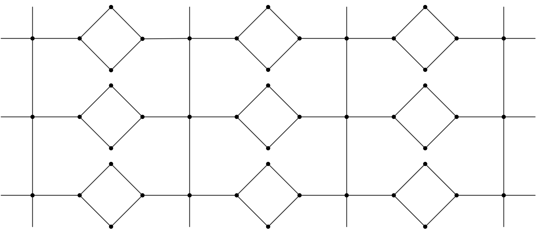
The fact that the graphing is hyperfinite and one-ended follows from the hyperfiniteness and one-endedness of . admits a perfect fractional matching which is a perfect matching on the -cycles and is equal to on the edges from . Note that a measurable perfect matching on would have to be a perfect matching on each -cycle and hence its restriction to the edges of would be a perfect matching in .
Now we describe the construction of a measurable bipartite graphing. It is based on the construction above and the second author’s construction from [Kun21]. Let be irrational and linearly independent over the rationals. Consider the following four isometries of the real line: , and the measurably bipartite graphing whose classes and are Borel isomorphic to the intervals and , respectively, and the set of edges corresponds to the union of the restrictions of the graphs of the four isometries. As shown in [Kun21], the graphing does not admit a measurable perfect matching. For every add a cycle of length to the graphing , and connect one vertex of the cycle to and the opposite vertex to . Denote the induced graphing by .
As before, the fact that is hyperfinite follows from the fact that a Schreier graphing of an action of an amenable group is hyperfinite. It is one-ended by Proposition 2.1, since every component of contains infinitely many components of .
Again, admits a measurable perfect fractional matching which is a perfect matching on the -cycles and is equal to on the edges from . Any measurable perfect matching on would have to be a perfect matching on each -cycle and hence its restriction to the edges of would be a perfect matching in . ∎
This example shows that it is possible to construct one-ended graphings and perfect fractional matchings that are forced to obtain specific values on some edges. After removing these forced edges, the remaining graphing may be two-ended and admit no measurable perfect matching. In order to avoid this problem we consider the following notion.
Definition 3.2.
Given a graphing , measurable and and a measurable perfect fractional -matching , the support of with respect to is
If is equal to everywhere, then we write for .
Now we can state our main theorem on rounding measurable perfect fractional matchings.
Theorem 3.3.
Let be a bipartite graphing be integrable and be measurable. Suppose that admits a measurable perfect fractional -matching such that is hyperfinite and nowhere two-ended . Then admits a measurable perfect -matchings bounded by such that . Moreover, belongs to the closure of the convex hull of such measurable perfect -matchings, with respect to the a.e. convergence.
In particular, Theorem 3.3 implies that under its assumptions a.e. edge in belongs to a measurable perfect -matching bounded by such that .
The support is defined above for a given perfect fractional matching. However, there is always an essentially largest such support for a given graphing, as shown in the next lemma.
Lemma 3.4.
Let be a graphing, and be measurable. If there exists a measurable perfect fractional -matching bounded by then there exists a measurable perfect fractional -matching bounded by such that for every measurable perfect fractional -matching bounded by the set is a nullset.
Proof.
We define a sequence of perfect fractional -matchings in the following way. Start with an arbitrary measurable perfect fractional -matching . Assume that given the measurable perfect fractional -matching there exists a measurable perfect fractional -matching that does not satisfy the condition of the lemma (with replacing ).
Consider , where the supremum is taken over all such perfect fractional -matchings , and pick a for which is at least the half of this supremum. Set . The sequence is uniformly convergent, and the limit is a measurable perfect fractional -matching bounded by . Note that . Hence satisfies the lemma by the choice of . ∎
Finally, as a corollary to Theorem 3.3, we can give our characterization of hyperfinite graphings with measurable perfect matchings — via a reduction to the two-ended case. Note that a measurable perfect fractional matching of essentially maximal support can be found effectively as in the proof of Lemma 3.4.
Corollary 3.5.
Let be a bipartite hyperfinite graphing, be integrable and be measurable. Let be a measurable perfect fractional -matching with essentially maximal support . The graphing admits a measurable perfect fractional -matching a.e. if and only if the two-ended components of admit a.e. a measurable perfect -matching.
Remark 3.6.
For the rest of this paper we will work under the assumption that that is the constant function , i.e., for every edge . Proving Theorem 3.3 under this assumption is sufficient, since for arbitrary measurable we can consider with and . We will also assume that as we can always replace with . Finally, we may also assume that for every vertex as we can work on the induced subgraph on .
Let us also comment on the assumption that is integrable in the results above. The only place when we essentially use this assumption is Section 7 (Claim 7.4). In all other results we can work without this assumption, replacing the (possibly infinite) measure with an equivalent quasi-invariant finite measure (as in the proof of Lemma 2.3)
When applied to a constant function , Theorem 3.3 gives the existence of measurable perfect matchings in a wide range of hyperfinite one-ended graphings, and Theorem 1.1 from the introduction is a special case of Theorem 3.3. Corollary 1.2 follows when applied to the perfect fractional matching that is equal to everywhere, where is the degree of the regular graphing. We will see some applications of Corollary 1.2 in Sections 9 and 10. Theorem 3.3 can also be applied to find regular spanning subgraphings of arbitrary degree in one-ended regular graphings. This, in particular, implies Corollary 1.2.
Corollary 3.7.
Any -regular hyperfinite one-ended bipartite graphing admits a -regular spanning subgraphing for every .
Proof.
Consider the functions on every edge, on every vertex and apply Theorem 3.3. ∎
We can also use Theorem 3.3 to obtain a measurable balanced orientation in a regular one-ended graphing of even degree, i.e., an orientation such that the in-degree equals the out-degree for every vertex (cf. [BHTb]). In [Tho22, Theorem 1.5] Thornton showed that any -regular Borel graph admits a Borel orientation for which the out-degree of every vertex is in . In case of regular graphings of even degree , Theorem 3.3 implies the existence of a measurable orientation, for which the out-degree of a.e. vertex is , so that it is a balanced orientation.
Corollary 3.8.
Consider a hyperfinite one-ended graphing . Assume that every vertex has even degree. Then there exists a measurable balanced orientation of the edges.
Proof.
Consider the barycentric subdivision of , that is, , and . Note that is a hyperfinite one-ended graphing. Consider the functions defined as for every , for every . The constant half function on is a fractional measurable perfect -matching. Hence, by Theorem 3.3 there exists an measurable perfect -matching bounded by . Consider the following orientation: an edge is oriented towards if . This is a balanced orientation. ∎
In particular, this answers the question of Bencs, Hrušková and Tóth [BHTb, Question 6.4], as it shows that every unimodular vertex-transitive graph of even degree without a factor of iid balanced orientation is quasi-isometric to . A factor of iid is defined for unimodular graphs (see [BHTb, Section 2.7]), and in the non-amenable transitive unimodular case, a factor of iid balanced orientation exists by [BHTa, Theorem 1], while in the amenable one-ended case it exists by Corollary 3.8. So this leaves only the two-ended graphs, which are quasi-isometric to by [MR, Corollary 3.13].
4. Rounding perfect fractional matchings and the matching polytope
If a finite bipartite graph admits a perfect fractional matching, then it admits a perfect matching. A very elegant proof of this fact, due to Edmonds, is obtained by looking at the so-called perfect fractional matching polytope of all perfect fractional matchings and noticing that an extreme point of this polytope must be a perfect matching. The latter follows from the fact that for an extreme point of the matching polytope the set must be acyclic. In this section, we exploit this idea in the context of measurable perfect fractional matchings.
Definition 4.1.
Given an even cycle in a graph with a distinguished edge and , an alternating -circuit on is a function that is equal to on the even edges and on the odd edges (even and odd edges with respect to their distance from the distinguished one).
First, the simple idea of constructing a measurable perfect matching for which is acyclic leads to a short proof of Theorem 1.3.
In the proof we use the following standard notation: given a sequence , we write and for the concatenations of with and , respectively. For we write for
Proof of Theorem 1.3.
We construct perfect fractional matchings for every such that each takes values in on every edge. We start with the empty sequence and put to be the perfect fractional matching that takes the value on every edge.
Suppose we have all for . For each such , using [KST99, Proposition 4.5] we can find a Borel set of disjoint cycles (each with a distinguished edge) whose edges are contained in . For each we choose a Borel set such that is equal to at least half of the supremum of the measures of for all possible such .
Next, we define and . To define we add an alternating -circuit to every cycle in , and to define we subtract an alternating -circuit to every cycle in .
Note that
| (4.1) |
Consider the probability measure space on with the symmetric flip-coin measure and the random variables and . Then by (4.1) we have
Since each is bounded by , the norms are bounded by and hence we get
which means that for a.e. the sum is finite. By the Borel–Cantelli lemma a.s. the value at a.e. edge will change only finitely many times in the sequence . Write for the limit and note that it is a.e. a measurable perfect fractional matching.
A.s. the set is essentially acyclic. Namely, we claim that is acyclic whenever the sum is finite. Indeed, otherwise we could find a family of pairwise disjoint cycles in whose union would have a positive measure. But this would contradict that , by our choice of close to the optimum.
A.s. in a.e. component of the set is a tree and has no leaves. By hyperfiniteness, the average degree of vertices in is equal to , so since it has no leaves, must be a disjoint union of lines in a.e. component. We know that has values which are rationals with denominator , hence on each line these values alternate between and for some natural number . Since is odd, this gives us a measurable choice of a perfect matching for a.e. such line and changing to such a measurable perfect matching on the lines gives a measurable perfect matching on the whole graphing .
∎
The next several sections will be devoted to the proof of Theorem 3.3. To this end, unless stated otherwise, we fix a hyperfinite bipartite one-ended graphing on and given an integrable we consider the following set
Clearly, is a convex subset of . It is bounded, as for , we have by the Hölder inequality and the fact that . Note that is closed in the weak∗ topology of . Hence is compact (as a bounded subset of ), separable and metrizable in the weak∗-topology.
The Krein–Milman theorem implies that is a convex closure of the set of extreme points, in particular, it contains an extreme point. While for finite graphs , any extreme point of must be a perfect matching, in the context of graphings the situation turns out to be a bit more subtle. In general, extreme points of do not need to be a.e. integral, as shown in Example 3.1. However, they have a nice structure, as we will see below.
Lemma 4.2.
Suppose that is a bipartite hyperfinite graphing, is an integrable function and is an extreme point. Then for a.e. we have
and the set is essentially a vertex-disjoint union of bi-infinite paths.
Proof.
First we show that the set of edges, where is not integral, is essentially acyclic. Suppose that the set of edges that belong to a cycle on which is not integral has a positive measure. We can assume that the measure is finite and positive and pass to a locally finite subgraphing spanned by cycles on which is not integral such that the measure of the edges in this subgraphing is positive. Using a Borel coloring of the intersecting cycles [KST99, Proposition 4.5], we would find an and a set of pairwise disjoint cycles of positive measure such that we could add or subtract alternating -circuits to on these disjoint cycles and still be in . However, this is not possible for an extreme point. Thus, the set of non-integral edges of is essentially acyclic.
Note that there is no vertex covered by exactly one edge where is not integral. Since the set of non-integral valued edges is acyclic and is hyperfinite, the subgraph spanned by these edges should have a.e. degree two or zero. Hence, the set of edges, where is not integral is essentially a vertex-disjoint union of bi-infinite paths.
On every such path alternates between two values. Consider the set of paths where is not half. If the set of such paths had a positive measure we could add or subtract for a possibly smaller set of paths of positive measure and an an alternating -valued measurable function to and still stay in , which is not possible for an extreme point. This completes the proof of the lemma. ∎
Throughout this paper, given a graphing and an integrable we write
Note that by Lemma 4.2, the extreme points of are in . For set
Later, we will prove that given a measurable perfect fractional -matching , we can find an extreme point such that has smaller measure than if the latter has positive measure.
5. Covering lines with cycles via connected toasts
In this section we start by constructing special tilings of one-ended hyperfinite graphings. We then use them to construct families of cycles in the graphings which cover given families of lines.
The construction of the tilings uses recent results of Timár [Tim19] and Conley, Gaboriau, Marks and Tucker-Drob [CGMTD] on measurable one-ended trees, expanding on prior work of Benjamini, Lyons, Peres, and Schramm [BLPS99]. The following definition refines the notion of a toast structure (see [GJKS18, Definition 2.9], [GJKS15, Definition 4.1]), coined by Miller and motivated by the work of Conley and Miller [CM16] (in particular, a toast structure is any tiling that satisfies Properties (1) and (2) of the definition below).
Definition 5.1.
Given a Borel graph , we say that a Borel collection of finite connected subsets of is a connected toast structure if it satisfies
- (1)
,
- (2)
for every pair either or , or ,
- (3)
for every the induced subgraph on is connected.
For a graphing , we say that it admits a connected toast structure a.e. if there exists a Borel co-null set such that there exists a connected toast structure for the graph .
Note that if admits a connected toast structure then it must also admit a Borel one-ended (component-wise) spanning tree. In the other direction, we may use one-ended spanning trees to construct connected toast structure a.e.
Proposition 5.2.
Any locally finite, one-ended hyperfinite graphing admits a connected toast structure a.e.
Proof.
Any hyperfinite one-ended graphing contains a.e. a measurable one-ended spanning tree with the same connected components as the graphing by [CGMTD, Lemma 2.10]11 1 In case of random amenable one-ended unimodular graphs, this was proved in [Tim19, Corollary 2]. Let be such a tree for . We say that a vertex is of height in if the maximum downward directed path in starting from is of length . We call a finite set a tile of height if it consists of a vertex of height and the vertices below it in . Further, we say that is covered by if .
First, we construct an increasing sequence of integers and a sequence of families of tiles such that
- (i)
the height of every tile in is at least and less than ,
- (ii)
for every ,
- (iii)
for every , the total measure of the tiles in which are not covered by a tile in is at most .
Towards this, observe that for any finite connected there are infinitely many integers such that is covered by a tile of height . Having defined and satisfying the desired properties (i)—(iii), we can find an such that
- •
all but an arbitrary small proportion of the tiles in are covered by tiles of height at least and less than
- •
all but an arbitrary small proportion of the vertices are contained by tiles of height at least and less than
Let consist of the maximal tiles of height at least and less than .
Now, we define as follows. A tile belongs to if there exists such that and is covered by a tile in
First, note that almost every vertex is contained in some tile of . Property (ii) of the construction and the Borel–Cantelli lemma show that a.e. vertex is contained by a tile in for all but finitely many . Property (iii) of the construction and the Borel–Cantelli lemma imply that for a.e. vertex all but finitely many tiles containing it are in .
For every edge there is a vertex such that the endvertices of are contained by a tile if and only if is in the tile. And for every vertex there are only finitely many such edges, hence (1) of the definition is satisfied for .
To obtain the connected toast strucutre, we will modify by gluing some tiles together, in order to ensure that property (2) is satisfied. More precisely, let be the relation that relates tiles and if but and let be the smallest equivalence relation on the set of tiles that contains . We put and we claim that is a connected toast structure.
The property (1) is satisfied for since it was satisfied for . Note that any two tiles are either disjoint or one contains the other. By construction, if a tile in contains another then it also covers it. Moreover, if covers then also covers . This implies that each element of is finite as well as the property (2) of the definition of a connected toast structure. The property (3) of the definition is satisfied because if , then is connected by the edges of the tree .
∎
In the remaining part of this section, we construct families of cycles in a graphing that cover a family of lines in that graphing. In particular, given an extreme point , this will allow us to cover the lines of with cycles. We will use this in the next sections to decrease the measure of until it becomes zero.
Lemma 5.3.
Consider a hyperfinite one-ended graphing and a subgraphing on . Assume that is the vertex-disjoint union of bi-infinite lines.
Then for every and there exist Borel families , each consisting of pairwise edge-disjoint cycles such that
- •
every edge not in is covered by at most one cycle in ,
- •
.
Proof.
We may assume that is locally finite and even , since contains a locally finite hyperfinite a.e. one-ended spanning subgraphing by Lemma 2.2, and we may consider the spanning subgraphing with edge set . Let be a connected toast structure for the graphing given by Proposition 5.2. Let denote the family of minimal sets (ordered by containment), denote the family of minimal sets in etc. Obviously, . Choose large enough such that at least of the edges of is contained by a set in . We construct for a family of pairwise edge-disjoint cycles contained in the sets of .
For every let denote the set of edges in with at least one end-vertex in . Note that is a.e. an edge-disjoint union of finite paths with end-vertices not contained by the sets of .
Since is connected, by Lemma 2.4 applied to the set of endpoints of , there exists a set of edges such that has vertices of even degree only, and . Note that is an edge-disjoint union of cycles and denote this collection of cycles by . For each we put to be the union of the families for in . Every such family contains all edges of , which has measure at least .∎
While the above lemma will suffice to obtain the results in the next section (in particular in case of a regular graphing), the general case will require a somewhat more subtle analysis. We will use the following definition to analyse general graphings.
Definition 5.4.
Assume that is a subgraphing of a graphing . We say that is one-lined if consists of a single connected bi-infinite line in every component.
The next two lemmas will be used to decrease the measure of for an extreme point in case is not one-lined. They will be used in the proof of our main results in the general case.
Lemma 5.5.
Let be a locally finite hyperfinite two-ended graphing and a subgraphing. Assume that is the vertex-disjoint union of bi-infinite lines and is nowhere one-lined.
Then for every and every there exist Borel families each consisting of pairwise edge-disjoint cycles such that
- •
every edge not in is covered by at most one cycle in ,
- •
.
Proof.
Note that a.e. component of contain only finitely many lines, since components with infinitely many lines have superlinear growth and thus are one-ended by Proposition 2.1. We can assume that all components have the same number, say , lines (by working separately with the union of the components with the same number of lines). By our assumption .
By Proposition 2.1, find a family of finite cutsets in such that cutsets are connected, each component of is connected and is adjacent to exactly two cutsets in . The family is bi-infinite on a.e. line of . Also, given we write for the set of vertices that lie on or between these two cutsets and , according to this bi-infinite structure. We also refer to the sets of the form as to intervals.
Given write for the vertices that lie on an interval of a line in such that the interval intersects only on its endvertices, one in and one in . By shrinking if necessary we can assume that for every the set is a disjoint union of exactly intervals of lines in .
We can find a Borel family of disjoint intervals of the form for such that more than of edges in lie on for being two endpoints of the same interval in .
Now we fix one and work locally on its induced subgraph. First, if is odd, then choose one of the shortest of the intervals in and remove it from . Write for without this chosen interval. Note that is a union of an even number of intervals in lines in .
Next, for find families of pairwise disjoint sets of the form such that taking the union of all for for all we still cover at least of the edges in . Moreover, since is obtained by removing at most one (among the shortest) of intervals from , and only when , we can ensure that the union of all (for and as above) will cover at least edges in .
The set is a union of an even number of intervals of lines in . Apply Lemma 2.4 to the endvertices of these paths in and , respectively, in order to get edge-disjoint cycles covering these paths with all the additional edges in and .
Write for the family of all cycles obtained in the above way for all for for all . Note that we cover all edges in that lie in , and the latter set has measure at least . ∎
Lemma 5.6.
Let be a hyperfinite graphing and a subgraphing of . Assume that is the vertex-disjoint union of bi-infinite lines and is nowhere one-lined. Let be integrable and be a measurable perfect fractional -matching.
There exist such that for every there exist Borel families , each consisting of pairwise edge-disjoint cycles such that
- •
every edge not in covered by at most one cycle of
- •
,
- •
for every edge covered by .
Proof.
Fix . Given consider the spanning subgraphing spanned by the set of edges . Note that is locally finite. Choosing small enough, we can make sure that the measure of the union of components of where is one-lined is arbitrarily small. We can apply Lemma 5.3 (with ) to the union of the one-ended components of and Lemma 5.5 (with ) to the union of two-ended components of in order to obtain the required family of cycles. ∎
6. Random distortions of perfect fractional matchings
Over the next couple of sections, we show how, given an extreme point of one can improve it in the way that the measure of can be decreased, until it becomes .
In this section, will first do it under the additional assumptions of Proposition 6.2, which will already suffice to obtain Corollary 1.2, as stated in Theorem 6.4. To prove it, we will study what happens when we randomly distort a perfect fractional matchings by adding to it small random numbers. We will use the following terminology.
Definition 6.1.
Suppose is a bipartite graphing, and is integrable. By a random measurable perfect fractional -matching we mean a Borel probability measure on .
Given a random measurable perfect fractional -matching on , and a real-valued function on , we write for the integral with respect to . Also, given a Borel probability measure on we will write for the barycenter of .
Proposition 6.2.
Let be a hyperfinite bipartite one-ended graphing, be integrable and be a measurable perfect fractional -matching such that .
Let be a measurable perfect fractional -matching such that and .
Suppose that at least one of the following holds
- (a)
is one-ended for some ,
- (b)
or is nowhere one-lined.
Then there exists a random measurable perfect fractional matching such that is an extreme point of a.s. and
- (i)
- (ii)
.
and is a convex combination of and .
Before we prove the proposition above, we state and prove the following lemma. Its statement is slightly stronger than what we need in this section (namely in Theorem 6.4 we will use it only in case is a measurable perfect -matching) but we will use this stronger statement in the next sections.
Lemma 6.3.
Let be a hyperfinite bipartite graphing and be integrable. Let be a measurable perfect fractional -matching such that and .
Suppose a random measurable perfect fractional -matching which is a.s. an extreme point of such that
Then the following hold.
- (i)
- (ii)
.
Proof.
Consider the sets (treated as random variables)
and note that (Technically, we will only treat and as random variables.) Note that by Lemma 4.2 we have
and
Write , so that we have
Now we prove the main result of this section.
Proof of Proposition 6.2.
By Lemma 6.3, it is enough to find a measurable perfect fractional matching which is a.s. an extreme point of such that
and is a convex combination of and .
First we find a measurable perfect fractional matching that satisfies the inequality, but may not be supported on extreme points.
There exists such that for every there exist Borel families of cycles , each consisting of pairwise edge-disjoint cycles and such that
- •
every edge not in is covered by at most one cycle of ,
- •
,
- •
for every edge covered by .
Indeed, if (a) is satisfied, then apply Lemma 5.3 to to , and the subgraphing spanned by for the given in (a). If (b) is satisfied, then apply Lemma 5.6 to and get such that the above are satisfied.
We choose large enough to be specified later and let be Borel families of cycles as above. Put
| (6.3) |
and consider the perfect fractional -matching
Note that for every edge covered by a cycle in we have
| (6.4) |
For every cycle in select one edge in a Borel way. For every we consider the alternating -circuit on the cycles in , i.e., is equal to 0 on edges that do not belong to such cycles and for every cycle in the function is an alternating -circuit on this cycle.
Let the random variables be independent identically distributed with . Write for the random perfect fractional -matching obtained by randomly adding the circuits on the cycles, i.e.,
Note that (6.3) imply that and thus by (6.4) we have that for . For we have and thus , so by (6.3) we also get . That means that is still in , for every choice of
Note that for every edge the value has the same sign, depending only on whether or , and thus implies that
| (6.5) |
For every measurable fractional perfect -matching we have , so, by (6.5) and Fubini’s theorem, in the expected value we have
| (6.6) |
Write and note that by the properties of our families of cycles. Recall that the Berry–Esseen theorem implies that if are iid with , then , where has normal distribution, and thus . Therefore, for every edge we have
| (6.7) |
and the exact value of in (6.7) does not depend on the edge , so by Fubini’s theorem we have
| (6.8) |
| (6.9) |
Note that the barycenter of is , since for each .
Now, we improve to be concentrated on the extreme points of . By the Choquet–-Bishop–de Leeuw theorem, there exists a probability measure on the set of extreme points of whose barycenter is .
Note that for a.e. either is always non-negative or is always non-positive. Hence its absolute value is linear and
On the other hand, for a.e. we have , so by convexity of on , Jensen’s inequality and Fubini’s theorem imply
∎
Using the previous proposition, we can state and prove the following weaker version of Theorem 3.3, which implies Corollary 1.2. The proof of Theorem 3.3 in Section 8 will basically follows the same lines but will need a more detailed analysis of Section 7 (this will be needed to prove Theorem 3.3 in its full generality, which is useful e.g. for applications such a those in [Tim21]).
Theorem 6.4.
Let be a bipartite hyperfinite graphing and be integrable. Suppose that admits a measurable perfect fractional -matching such that for some the set
Then admits such a measurable perfect -matching .
Theorem 6.4 can be strenghtened to say that is equal to a barycenter of a probability measure on concentrated on the set of measurable perfect -matchings, see Remark 8.2 after the proof of Theorem 3.3.
Proof.
We will find a perfect -matching in .
By the Krein–Milman theorem, there exists which is an extreme point of . Starting with , by induction, we define a sequence of measurable perfect fractional -matchings for countable ordinals , so that
- (i)
if ,
- (ii)
,
- (iii)
for limit .
Suppose we have constructed . By Lemma 6.2 there exists a random perfect fractional -matching concentrated on such that
Since is concentrated on , there exists an extreme point of for which
Using Lemma 6.3 (treating as a Dirac random perfect fractional matching) we get (i) and (ii) as needed.
At limit stages , note that the condition (i) implies the sequence for is strictly decreasing and (ii) implies that is a.e. convergent by the Borel–Cantelli lemma. We put to be the limit of this sequence.
Note that there must exist , such that have and then this is a measurable perfect -matching a.e. as needed.
∎
7. The one-lined case
For extreme points of which are one-lined, we will need a slightly different argument in order to decrease . The goal of this section is to prove the next proposition, which is a version of Proposition 6.2 in the one-lined case.
Proposition 7.1.
Let be a bipartite one-ended graphing and be integrable. Suppose that is a measurable perfect fractional -matching such that and . Assume that is one-lined on a set of components of positive measure. Let .
There exists a random measurable perfect fractional matching which is a.s. in such that
- (i)
- (ii)
.
and .
The key to prove Proposition 7.1 is to find a family of cycles we can use for the rounding. First, we need to introduce some notation.
Definition 7.2.
Let be a bipartite graphing and be integrable. Suppose is an extreme point of such that is one-lined everywhere.
- (i)
Write and .
- (ii)
A -augmenting path is a path of odd length such that we have for and for .
- (iii)
A -augmenting cycle is a cycle obtained by joining a -augmenting path with endvertices on and the finite subinterval of joining the two endpoints of the -augmenting path.
- (iv)
For a -augmenting cycle we write for the set of edges of that contains every other edge of extending , and analogously we define .
- (v)
-augmenting cycles in the same component of can be naturally divided into two equivalence classes induced by the proper -coloring of the edges of the infinite line (this is done in the single component). Two -augmenting cycles and are equivalent if every has the same color as every edge in (and the same holds for and ).
In particular, the definition of a -augmenting path requires that all vertices along the path are distinct. Note, however, that since the graphing is bipartite, any walk satisfying the conditions of (ii) above contains a -augmenting path obtained by removing the (even) cycles between repetitions of vertices. Note also that there are exactly two equivalence classes of -augmenting cycles.
The following lemma gives us the family of cycles that will be useful in proving Proposition 7.1.
Lemma 7.3.
Let be a bipartite one-ended graphing and be integrable. Let . Suppose that is one-lined everywhere and there is no subset of of positive measure that admits a measurable perfect matching.
For every and there exists measurable collections each consisting of -augmenting cycles edge-disjoint in both equivalent classes such that
- •
every edge not in is covered by at most four -augmenting cycles in ,
- •
for each , every edge in is covered at most twice by -augmenting cycles in ,
- •
in both equivalence classes in .
Proof of of Proposition 7.1.
By Lemma 6.3, it is enough to find a random measurable perfect fractional matching which is a.s. in such that
| (7.1) |
and .
First, suppose that there is a subset of of positive measure such there is a measurable perfect matching on . Let be uniformly distributed and define as follows. For edges let if belongs to the perfect matching, and if does not belong to the perfect matching, while for let . Note that and the left-hand side in (7.1) is zero, while the right-hand side in (7.1) is positive, so is as needed.
Thus, for the rest of the proof we can assume that there is no measurable perfect -matching on any subset of of positive measure
Write for the union of the components of where consists of a single line. Let . By our assumption, .
Let be big enough and be small enough. Apply Lemma 7.3 to get families of -augmenting cycles such that every edge is covered by at most four -augmenting cycles in and for every every edge in is covered by at most two -augmenting cycles from , and all but edges from are covered by exactly one -augmenting cycle from each equivalence class in .
We may assume that the cycles in have bounded length. Using [KST99, Proposition 4.6], we can find and partition into edge-disjoint Borel subfamilies .
For each we define the function as follows. and is equal to on the edges that do not belong to and for every -augmenting cycle the function is a -circuit on , where the chosen edge is belongs to .
Let be a random variable with the uniform distribution and let be an independent random variable with the uniform distribution. Consider the following random perfect fractional matching
Note that
| (7.2) |
as a.e. edge in is covered at most four times by . Thus, by (7.2)
| (7.3) |
since for every edge we have .
Note also that for every edge covered by we have
| (7.4) |
with probability . Thus, by Fubini’s theorem we get
| (7.5) |
which follows from (7.4) and the fact that . The latter is true because every family covers up to .
To see that (7.1) is satisfied, note that by (7.3) and (7.5) we get
| (7.6) |
which is positive as long as is big enough and is small enough.
Now let us look at the barycenter of . Write is covered by one cycle as a edge and by one cycle as a . By our assumption, we have . Note that the barycenter can change only at the edges in edges in and at the edges in covered by . Each of the former edges is covered at most times and the measure of such edges is at most . Each of the latter edges is covered at most four times and their measure is at most . The absolute value of the change is with probability . Thus, we get . Thus, by (7.6) we are done if , which holds if is big enough and is small enough, relative to .
∎
The rest of this section is devoted to the proof of Lemma 7.3.
Proof of Lemma 7.3.
We will need a series of claims.
Claim 7.4.
A.e. vertex in is available via a -augmenting path from and has an -neighbor available via a -augmenting path from .
Proof.
Write for the set of vertices available via an augmenting path from and for the set of vertices in not adjacent to a vertex in via an edge in . Also, denote by the set of neighbors of via an edge in . We will show that is co-null and both and are null. This will be enough since every vertex has an -neighbor (recall that ).
We have and and we will show that both and have measure zero. By the definition of , for every edge from to the complement of we have . Note that every -edge from goes to , since there is a -augmenting path to its other endvertex. Moreover, every -edge from goes to , else there would be a -augmenting path to its endvertex in . The latter implies that for every edge from to the complement of we have . In other words, for all and for all .
Recall that for every set and every measurable perfect fractional -matching we have . Then we can write as
Since the first expression is maximal among the values where is replaced by another perfect fractional -matchings, we must have for a.e. and for a.e. . However, by our assumption happens on a null set of edges . Thus, . The set is disjoint from , which implies that is a nullset.
Now, since is a nullset essentially every edge leaving is not in , or else the other endvertex would be available via a -augmenting path from . In other words for every edge . Let and note that every edge from must go to , since there is a -augmenting path to its other endvertex. Thus for every edge . As previously, we can write as
Again, since for all , the left hand side is maximal possible among the values where is replaced by another perfect fractional -matching bounded by , we must have for a.e. . Hence is a nullset. Therefore a.e. vertex belongs to . ∎
Claim 7.5.
For a.e. component of , for every finite subset of the following is true
- (1)
All but finitely many vertices of are available from via a -augmenting path contained in and have an -neighbor available from via a -augmenting path contained in .
- (2)
For every finite interval there exists a -augmenting path connecting the two semi-infinite paths of in .
Proof.
By Claim 7.4 we can assume that every vertex in is available via an augmenting path from and has an -neighbor available via such a path.
(1) For every positive integer consider mapping to the -th vertex of the lexicographically first (with respect to any Borel coloring of directed edges with natural numbers) shortest augmenting path from to . Write for the graphing where we put an edge between and for every . Note that is acyclic because is bipartite and thus the -component of every point in is a tree. Let denote the set of points in whose -component is infinite. We claim that has measure zero. Towards a contradiction, suppose that has positive measure. For each positive integer let be a Borel function on such that is an element of the -component of , for , and for . Considering the disjoint sets we get a contradiction by the assumption that the graphing is pmp, as the sets must have equal measure.
Thus, for a.e. point in its -component is finite. Given any finite set , the union of -components intersecting is then finite, as well as the set consisting of all -neighbors of vertices in . Since every vertex has at least one -neighbor (recall that ), any vertex which is not in satisifes (1).
(2) By (1), all but finitely many vertices are available from via a -augmenting path contained in and have an -neighbor available from by such path. Let denote the set of such vertices available from one of the semi-infinite paths of and the set of vertices available from the other semi-infinite path. Every vertex has an -neighbor which is in . If and available from different infinite-subpaths, then we can join their -augmenting paths via and obtain a -augmenting path disjoint from joining the two semi-infintie paths of . So we can assume that for every vertex each its -neighbor which is in is available from the same semi-infinite path of .
If , then let . Choose a -neighbor of such that . We can then find two -augmenting paths disjoint from joining and with distinct semi-infinite paths of and joining them along gives us the desired path.
Thus, suppose that and are disjoint. Put . is finite and since is one-ended and each contain a semi-infinite path, we know that there are infinitely many edges with , and in particular there is such an with neither of its endvertices in . If then joining the augmenting paths to and via gives the desired augmenting path joining the two semi-infinite paths. If then, by our assumption, we can find -neighbor of and of . Joining the -augmenting paths to and with the three edges , and gives us the desired path.
∎
Claim 7.6.
For almost every component of , for every finite interval and every finite subset there are -augmenting cycles in both equivalence classes covering and disjoint from .
Proof.
Let be the set of those edges in such that it is not the case that for every finite interval containing and every finite subset of there are -augmenting cycles in both equivalence classes covering and disjoint from .
Note that for each line in either the line is contained in or disjoint from . Thus, we need to show that the set of lines contained by is a nullset. Part (2) of Claim 7.5 implies that in a.e. component for every finite subset disjoint from the line, every finite subinterval of the line can be covered by a -augmenting cycle in one of the equivalence classes disjoint from this set. If a line in in such a component is contained in , then for every edge in that line there is a finite interval containing and a finite subset of that component such that exactly one of the followings holds:
- (a)
either for every -augmenting cycle covering and disjoint from we have
- (b)
or for every -augmenting cycle covering and disjoint from we have .
Note that this partitions a.e. edge of into type (a) or (b), and gives a measurable perfect matching on , contradicting our assumption. ∎
Given two -augmenting cycles that share the same edge, we will want to obtain a -augmenting cycle that uses that edge and parts of the two cycles. In order to define this correctly, we need the following definition.
Definition 7.7.
Given two equivalent -augmenting cycles, we say that an edge not in belongs to their substantial intersection, if considering the orientations of the subpaths of the cycles on the line towards the same end, the extension of these orientations outside agrees on this edge.
Note that in the above definition it does not matter which orientation of the line we choose.
Crucially, note that if two equivalent cycles have an edge in their substantial intersection, then they can be merged into one -augmenting cycle in (possibly) four ways as follows. Let and be two equivalent -augmenting cycles and be an edge in their substantial intersection. Orient the subpaths of the cycles and on the line towards the same end and extend this orientation outside to the union of the -augmenting paths. Using this orientation, write for the subpath of starting at the vertex on the line preceding in the orientation and ending at a vertex of . Similarly define as the subpath of starting at a vertex of the edge following in the orientation and ending at a vertex of the line. Define and similarly for . To merge and we define the -augmenting path that starts with either or , is followed by and then by either or . Then we close this -augmenting path with the interval on between its endvertices.
Claim 7.8.
Let be a finite collection of equivalent -augmenting cycles that do not have substantial intersection outside and be a -augmenting cycle. Let be a finite interval such that and . Then there exists a -augmenting cycle obtained by merging with at most two cycles and of such that , and the cycle does not have substantial intersections with cycles in .
Proof.
Note that divides into two infinite components, so we refer to these two components as to the two sides of . For simplicity, suppose that there are -augmenting cycles in with vertices on both sides of which are equivalent to and substantially intersect on (if such cycles have vertices on only on one side of , then the proof is analogous to the proof below).
Choose -augmenting cycles and in with vertices on on different sides of such that is equivalent to and , substantially intersects at an edge and at an edge and the edges between and in do not belong to the substantial intersection of and any cycle in equivalent to . We merge , and as follows. Outside of the line we first take the edges of , followed by the edges of between and and then followed by the edges of outside of . This is a -augmenting path joining two vertices of and in order to get a -augmenting cycle we add the vertices of the interval of between these vertices.
Note that covers since and are disjoint from and on different sides of . Note that the cycle does not intersect substantially any equivalent cycle in on since cycles from do not have substantial intersections between equivalent cycles outside of the line. ∎
Now, we prove the statement of Lemma 7.3. More precisely, by induction on we prove that for every there exist Borel families of -augmenting cycles such that
- •
there are no edges in that belong to a substantial intersection of equivalent cycles in ,
- •
for every there are no edges on that belong to an intersection of equivalent cycles in
- •
in both equivalence classes in .
Note that this will imply the statement of Lemma 7.3 since there are two equivalence classes of -augmenting cycles and if an edge belongs to an intersection of three equivalent -augmenting cycles, then it belongs to a substantial intersection of two of them.
Assume that the statement holds for , and let the families be given by the induction assumption for . We will construct the families that work for . We choose a large and for each we construct families as well as a family such that
- (i)
and for each and ,
- (ii)
each equivalence class of -augmenting cycles in is disjoint on and covers at least edges in
- (iii)
for each the family does not have substantial intersections of equivalent cycles outside of .
Choose large enough such that and set and for each .
We construct the families by induction on . Suppose that they are constructed for a certain . Let and ( depending on ) be large enough.
Using Claim 7.6 choose a family of -augmenting cycles such that a.e. interval of length at least is covered by both equivalence classes of -augmenting cycles in which are disjoint outside of from those cycles of which intersect that interval. Next, find a family of finite subintervals of each of length at least and covering all but a small proportion of such that the cycles from that intersect distinct intervals from are disjoint.
Now, until further notice, we work locally on each .
We can assume that equivalent cycles in do not substantially intersect outside of . This can be ensured, as we can merge such cycles and still cover the same edges on the line.
Next, apply Claim 7.8 to each cycle intersecting to get a cycle obtained by merging with at most two cycles from . Note that by our assumption such cycles still cover (in both equivalence classes) the same intervals of length as the original cycles . Write for the family of such cycles . Note that if two equivalent cycles from cover disjoint subintervals of , then they must be obtained by merging distinct cycles to members of , and thus must not have substantial intersections outside of the line , by our assumption on and .
Now, divide into two families — the intersection with the two equivalence classes of -augmenting cycles. To each of those families apply Helly’s theorem to shrink it so that each edge of the line is covered by at most two -augmenting cycles of this shrunken family. Next, shrink both families again by taking every other -augmenting cycle in each of them and write for the family of -augmenting cycles in the union of both shrunken families. Note that we can make sure that
- (a)
the equivalent -augmenting cycles from cover pairwise disjoint intervals of the line,
- (b)
each equivalence class of -augmenting cycles in covers at least a half of .
The condition (a) follows since we have two ways of taking every other -augmenting cycle after applying Helly’s theorem. The condition (b) can be arranged if is chosen large enough. Note that by (a) and the property of the family , we get that equivalent -augmenting cycles from do not have substantial intersections outside of .
Now we leave the interval and work globally again.
For each shrink to and to by removing corresponding to the -augmenting cycles in for all . Note that the condition (i) can be arranged if is chosen large enough.
Finally, let consist of the -augmenting cycles from as well as the -augmenting cycles from whose interval does not intersect an equivalent -augmenting cycle from . Note that the condition (ii) can be arranged if is large enough.
∎
8. Improving random perfect fractional matchings
This sction is devoted to the proof of Theorem 3.3, which will follow the same lines as the proof of Theorem 6.4 but will need one more technical lemma.
Note that is closed in in the norm. We will consider with the induced distance. Note that is also closed in with respect to the norm. For the rest of this section, we consider as a Polish metric space with this induced metric.
Since the weak∗ topology on is also Polish and is weaker than the norm topology on , both topologies induce the same Borel structures by [Kec95, Theorem 15.1]. Thus, a Borel probability measure on the extreme points of is also a Borel probability measure on with the metric. We will consider the space of Borel probability measures on with the Wasserstein distance, induced by the metric on .
Lemma 8.1.
Let be a hyperfinite bipartite one-ended graphing and let be integrable. Suppose there exists is a measurable perfect fractional -matching such that .
Let be a random measurable perfect fractional -matching such that a.s. . Assume that . Let . Then there exists a random measurable perfect fractional matching which is a.s. an extreme point of and such that
- (i)
- (ii)
- (iii)
Proof.
We will replace the random perfect fractional matching with a perfect fractional matching on a larger graphing. Consider the graphing with the vertex set , where two vertices are adjacent if their first coordinates are equal and the second coordinates are adjacent in . Note that and naturally extend to and on and , by ignoring the first coordinates. Note that random perfect fractional -matchings correspond on correspond to perfect fractional -matchings on . Write for the perfect fractional -matching on corresponding to . The measure on and the measure on induce a measure on , which we denote by . Note that by our assumption.
Now we apply Proposition 6.2, in case is nowhere one-lined, and Proposition 7.1 in case is one-lined in a set of components of positive measure, to obtain and a random perfect fractional -matching on such that
- (i*)
- (ii*)
.
- (iii*)
Also, we set to be the random perfect fractional -matching on corresponding to . This means that is obtained by first choosing a random perfect fractional matching on , distributed according to , followed by randomly choosing , distributed according to and then restricting the perfect fractional matching on to the -th section of the graphing .
The condition (i) follows from (i*) and the fact that
| (8.1) |
Note that the barycenter of is obtained by taking the expectation of over . Note also that taking the expectation of over gives us the barycenter of , and the expectation of over is equal to . Thus (iii) follows from (iii*) and the Cauchy–Schwartz inequality:
For each we write for the corresponding random perfect fractional -matching on . More precisely, for each and a perfect fractional matching on we get the perfect fractional matching obtained by restricting to the -th section of the graphing . Then the measure is obtained as the pushforward of from to via the map . Note that can be represented by first randomly choosing , distributed according to , and then randomly choosing the perfect fractional matching, distributed according to .
In order to obtain (ii) and bound , consider the measure on which for is defined as (here we write for the -th vertical section of ).
Now we are ready to prove our main Theorem 3.3.
Proof of Theorem 3.3.
By Remark 3.6, we can assume that is the constant function and is nowhere two-ended..
By [JKL02, Lemma 3.21(i)] on the union of infinite zero-ended components we have a measurable selector, so this union is a nullset. Thus, we can assume all zero-ended components are finite. For finite bipartite graphs the existence of a fractional perfect -matching is equivalent to the existence of a perfect -matching, so we can assume that is nowhere zero-ended, hence a.e. one-ended.
We will show that can be approximated by convex combinations of measurable perfect -matchings in . This will be enough since a sequence convergent in contains a subsequence convergent a.e.
Denote by the set of all measurable perfect -matchings on . We consider with the -metric. Note that is closed with respect to the norm so it is a Polish space as well (and we are about to show that it is nonempty).
We will show that for every there exists a random perfect -matching (i.e., a random perfect fractional -matching concentrated on ) such that . To see that this is enough, note that can be approximated in by convex combinations of elements of . Indeed, convex combinations of Dirac measures on are dense in the weak topology on , so there is a sequence of such convex combinations converging to in . This implies that the sequence converges to also in the weak topology of . Then is a limit of convex combinations of elements of in . By Mazur’s lemma there is a sequence of convex combinations of elements of converging to in .
Fix . By the Choquet–-Bishop–-de Leeuw theorem, is the barycenter of a measure on the set of extreme points of . Starting with , by induction, we define a sequence of random measurable perfect fractional -matchings concentrated on for countable ordinals , so that
- (i)
,
- (ii)
,
- (iii)
for any limit ordinal .
- (iv)
At every step we will have
- (v)
At successor stages, given , we use Lemma 8.1 to find .
For limit ordinals the condition (i) implies that the sequence for is strictly decreasing, and (ii) implies that is Cauchy w.r.t. the Wasserstein distance. Thus, we can set to be the weak limit of this sequence. In particular, we have in , so in . Note that we have since is continuous on with the distance. Finally, as balls are closed in the weak∗ topology, (v) follows.
Note that there must exist , such that have . This implies that the random perfect fractional -matching is a.s. a measurable perfect -matching a.e. Finally, the condition (v) implies that , which ends the proof.
∎
Remark 8.2.
Under the assumptions of Theorem 6.4 (so in particular for regular graphings), the proof of Theorem 3.3 above shows that can be made equal to a barycenter of a probability measure concentrated on measurable fractional perfect -matchings. This is because under the assumptions of Theorem 6.4, in Lemma 8.1 above in place of (iii) we get that is equal to a convex combination of and , since we can use Proposition 6.2 only and do not need to refer to Proposition 7.1.
9. Factor of iid perfect matchings
In this section we prove Theorem 1.4. The following will be the key lemma in the two-ended case.
Lemma 9.1.
Consider a group , where is a finite group, with a finite symmetric generating set for such that the corresponding Cayley graph is bipartite.
- (i)
If has odd order and is an a.e. free and totally ergodic action on a standard probability space, then its Schreier graphing does not admit a measurable perfect matching,
- (ii)
If has even order and is a free Borel action, then its Schreier graphing admits a Borel perfect matching.
Proof.
Since , there exists an element such that generates this quotient. Note that acts on and the Cayley graph of is a disjoint union of copies of arranged in a bi-infinite line . Also, since the cyclic group generated by is of finite index, it has a further finite index subgroup , generated by for some , such that is normal in .
(i). First, consider the case when is odd. Recall the following folklore fact.
Claim 9.2.
If is the Schreier graphing of a free totally ergodic action of with respect to as generating set, then does not admit a measurable perfect matching.
Proof.
Suppose admits a measurable perfect matching. The set of vertices is invariant under . Thus, it is either null or co-null by total ergodicity. However is obtained by shifting by . ∎
Now, let be a.e. free and totally ergodic. Assume is a measurable perfect matching. Note that on each orbit (which we identify with the Cayley graph of ), for every exactly one of the two sets of edges or has odd size. Write for the quotient of by the action of the group and note that is also a standard probability space. Note that the action induces the action and we consider the Schreier graphing of the action with respect to the generators . Consider the set of edges of that on every orbit contains if is odd. Note that is a measurable perfect matching in . The action is totally ergodic since is totally ergodic. This gives a contradiction by Claim 9.2.
(ii). Now assume that is even. We consider a bipartite Schreier graph of a Borel action , induced by a set of generators .
Claim 9.3.
In the Cayley graph of either is entirely contained in one of the class of the bipartition, or it contains an equal number of vertices from both classes.
Proof.
Note that the set of elements of which have even word length in the Cayley graph forms a subgroup of . Elements of lie in the same class of the bipartition as the neutral element, while the elements of lie in the other class. As is a subgroup of index at most , either it is equal to or constitutes half of its elements. ∎
Write for the quotient of by the action of the group and note that is also a standard Borel space. Recall that is a generator of such that . Consider the graphing on induced by the generator . Let . Note then that for every generator we have for some .
Claim 9.4.
There exists a finite subset containing the identity such that
- •
the induced Cayley graph on admits a perfect matching,
- •
the induced Cayley graph on the complement of in admits a perfect matching,
- •
the complement of in consists of two infinite connected components.
- •
if is such that , then the complement of consists of two infinite and one finite component, and the latter has half of its vertices in each class of the bipartition.
Proof.
By Claim 9.3, we consider two cases.
Case 1. Suppose that each copy of in contains an equal number of vertices from each class of the bipartition. Then we choose to contain copies of starting from the identity. We divide into consecutive unions of consecutive copies of . The perfect matching on each such consecutive union of copies of is induced by . Note that it can be extended to the left and to the right also using in the same way.

If is such that , then the finite component of the complement of is a union of copies of , so contains an equal number of elements of each class of the bipartition.
Case 2. Suppose that each copy of is contained in one class of the bipartition. Then we choose to contain consecutive copies of , starting at the identity, together with halves of copies of preceding them as well as halves of copies of following them. The perfect matching on is induced by so that on every copy of intersecting the block half of the vertices is matched in the direction and half in the direction (in the first halves we only use the direction and in the last halves we only use the direction). Note that this matching can be extended to the left and to the right to a perfect matching in the same way.

Suppose that is such that . To see that the finite component of the complement of contains an equal number of elements of both parts of the bipartition, note that it is the union of fragments of -orbits on the copies of , and on each such fragment the classes of the bipartition alternate between the copies of . In each such fragment, the vertices in the halves of the copies of on the boundary of the component of make up the difference in the number of vertices in each class of the bipartition.
∎
Let be such as in Claim 9.4 and be such that whenever , then . For sufficiently large, to be determined later, construct a maximal Borel -discrete set in the graphing (i.e., any of its two vertices are of distance at least and is maximal with this property, see [KM04, Lemma 7.3]). Consider the corresponding collection of representatives of copies of on orbits in and let .
Note that on each component of , the induced Cayley graph on has finite components, such that each such finite component has a perfect matching, and its complement also has a perfect matching. Also, the induced Cayley graph on the complement of has finite components which contain an equal number of elements from each class of the bipartition. We will refer to the finite components of as to blocks and to the finite components of the complemement of as to gaps. We clearly have a Borel perfect matching on the union of blocks. If we can extend this perfect matching in a Borel way to the gaps, then we will be done.
Given a gap, we use the convention to enumerate full copies of contained in the gap (say from left to right) as (for some ). First, we need the following claim.
Recall that was chosen so that generates a normal subgroup of .
Claim 9.5.
Fix a gap and let be contained in one class of the bipartition. If with and are such that
and is a proper nonempty subset of , then
Proof.
Write . Since , we get that . Consider the Cayley graph of and note that is a regular finite bipartite graph, so it admits a perfect matching. This implies that holds.
However, if then the Hall condition would be sharp for a proper nonempty subset in , and this contradicts the connectivity of .
So we get that that . ∎
Now we show how to extend the perfect matching to the gaps.
Claim 9.6.
If is large enough, then each gap admits a perfect matching.
Proof.
Let be a gap. In order to show that admits a perfect matching, we have to check Hall’s condition for . Note that since satisfies Hall’s condition, the only way that may fail is from the loss of edges leaving . There is an upper bound on the number of such edges that is independent of the size of . We will show that as long as is large enough this loss is overcome by extra edges between the inner copies of in . Consider a subset contained in one class of the bipartition, and suppose for a contradiction that .
If is large enough, then we choose such that and and
Write .
Note that intersects each , because otherwise would be partitioned into two sets far from each other such that one of them does not satisfy the Hall condition, contradicting the fact that the set of all vertices to the left or right of a given block can be extended to a perfect matching. Similarly, can not contain its entire class in , as we could apply the same argument to the complement of in the other class, using the fact that has the same number of elements from both classes of the bipartition.
This implies that for each , making up for the loss of edges leaving , which means that , as needed.
∎
Choosing big enough as in Claim 9.6, we can construct a Borel perfect matching in , which ends the proof.
∎
In the amenable case of Theorem 1.4, we will use the following proposition.
Proposition 9.7.
Let be a finitely generated amenable group and let be a bipartite Schreier graphing of an a.e. free action of
- •
If is isomorphic to for a finite normal subgroup of odd order and the action is totally ergodic, then does not admit a measurable perfect matching.
- •
If is not isomorphic to for a finite normal subgroup of odd order, then admits a measurable perfect matching.
Proof.
If is amenable and one-ended then the existence of a measurable perfect matching follows from Corollary 1.2.
Thus, we need to consider the two-ended case. Recall (see [SW79, Theorem 5.12]) that there exists a finite normal subgroup such that is either isomorphic to or to . In the first case, is isomorphic to for a finite group , and Lemma 9.1 implies the theorem.
Now assume that is isomorphic to . Note that the group has a normal subgroup of index two isomorphic to , and the elements not in this subgroup have order two. Hence there exists a generator defining the Cayley graph of whose image in has order two, hence has finite, even order. The Cayley graph of decomposes into -cycles of even length and the same is true for the graphing , so it admits a measurable perfect matching.
∎
Now we prove Theorem 1.4.
10. Measurable circle squaring
Recall that the circle squaring problem of Tarski [Tar25] asked if the unit disc and the unit square are equidecomposable. A positive answer was given by Laczkovich [Lac90] and recently Grabowski, Máthé and Pikhurko [GMP17] have given a measurable equidecomposition. We show a couple of different ways to deduce the measurable circle squaring from the main results of this paper.
In applications to equidecomposition problems, we consider measurably bipartite graphs. We will use the following notation. Given two disjoint sets of a metric space write for the bipartite graph whose vertices are and edges join two points, one from and one from at distance at most . In particular, if is a finitely generated group and is the metric on its Cayley graph with respect to a finite generating set , then for two disjoint subsets we denote the above bipartite graph by , Similarly, if is a free action, is a finite generating set and are disjoint, then we consider the bipartite graph (measurably bipartite if are measurable) whose vertices are and edges join two points in the same orbit if their distance in the Schreier graph is at most .
We will be interested in the graph obtained from the action of on the torus constructed by Laczkovich [Lac90], for a suitably chosen , where and is the standard set of generators of .
10.1. A proof of the measurable circle squaring using regular bipartite graphs
In this proof we directly use our perfect matching theorem 1.1. We show that the graph corresponding to the action of constructed by Laczkovich [Lac90] is very close to a regular graph. More precisely, using his construction, we consider a regular subgraph of the Schreier graphing of . Even though that graph is not measurable, we use a sandwich-type argument to approximate it with measurable graphings and apply Theorem 3.3.
Recall [Lac92b] that a set is uniformly spread with density if there exists a bijection such that . Uniformly spread sets can be defined in many equivalent ways [Lac92b, Theorem 1.1]. In the proof of the circle squaring, Laczkovich constructs an action of so that both the unit disc and the unit square are uniformly spread on each orbit. More precisely, given a free pmp action for each we identify the orbit of with in a canonical way. We say that a measurable set is uniformly spread with density (with respect to the action ) if for each there is a bijection between (identified with a subset of ) and such that . The Laczkovich theorem (more precisely, the combination of the Laczkovich Bijection Lemma [TW16, Lemma 9.8] and [TW16, Theorem 9.12, Claim 2]) shows that the measurable sets in the circle squaring are uniformly spread with respect to an action of .
Below, we write for the standard set of generators (the unit vectors). Given we write for . In the following proposition we construct a perfect fractional matching that is not necessarily measurable but it is defined on a measurable one-ended graphing and its support contains a measurable one-ended graphing.
Proposition 10.1.
Let . Consider a free pmp action and suppose that are measurable and uniformly spread with density . Then there exist such that the graph is one-ended and admits a perfect fractional matching that is constant and positive on the edges of .
Proof.
First, fix an orbit of the action of . Note that the embedding of into is a quasi-isometry and on the natural Cayley graph metric is equivalent to the Euclidean metric (induced by this embedding). Below, slightly abusing the notation, for subsets we write for the graph with edges () if the Euclidean distance of and is at most .
There is a perfect matching between and , and between and . Both matchings match each vertex to a vertex such that is bounded by a constant, since we assume that and are uniformly spread.
Note that the graph is regular for every . The matching between and allows us to identify the elements of and , and similarly, the matching between and allows us to identify the elements of and . We obtain using this identification that for every there exists such that all edges in are still edges in , and similarly, all edges in are still edges in .
Choose large enough such that is one-ended. Put , , .
Note that the graph is regular and let be its degree. Now, we can transport the constant fractional matching on to using the identification of with and with (i.e. we put on every edge between and if is identified with , is identified with and there is an edge between and ). Note that it is equal to on all edges from . is also one-ended, as it contains a subgraph quasi-isometric to via the identification of with and with . Finally, put , .
Note that since we do not require that the perfect fractional matching is measurable, we can define it separately on each orbit . However, the choice of and does not depend on the choice of the orbit since we assumed that and are uniformly spread with respect to the action .
∎
Theorem 10.2.
Let . Consider a free pmp action and measurable and uniformly spread with density . Then and are equidecomposable using measurable pieces.
Proof.
Corollary 10.3 (Measurable circle squaring).
Let be such that and . Then and are measurably equidecomposable.
10.2. A proof of the measurable circle squaring using two independent equidecompositions
In this proof of the measurable circle squaring we use Theorem 3.3 and the fact that circle squaring is possible by a large set of random translations (with high probability), as proved by Laczkovich.
Proposition 10.4.
Let be an amenable group, be its subgroups and be a probability measure preserving free action of on a probability measure space . Assume that for every the intersection is finite. Let be measurable and . If and admit an equidecomposition both by and then they admit a measurable -equidecomposition.
Proof.
We may assume that the groups are finitely generated and is the subgroup generated by . Let denote the set of generators of for . Let be such that and are equidecomposable using elements of of length at most with respect to . For consider the bipartite graphings , each with vertex set . We apply Lemma 2.3 to the graphings (with the subgraphs being empty) to get measurable perfect fractional matchings and of and in both graphings and respectively.
Now, let be the spanning subgraph of that consists of the edges where is positive. And let denote the spanning subgraph with edge set . We will prove that and admit a measurable perfect matching in . Note that is a measurable perfect fractional matching which is positive on all edges in .
First, for we show that the -components that contain infinitely many infinite -components are one-ended. By Proposition 2.1 it suffices to show that the growth of the balls in these components is superlinear. Given a vertex and if the radius is large enough then intersects more than infinite -components, hence . Since this holds for every these components have superlinear growth. We can apply Theorem 3.3 to the union of these -components and in order to get a measurable perfect matching.
Next, for consider the union of the -components that do not contain an infinite -component. These have only finite -components with a measurable perfect fractional matching, hence they admit a measurable perfect matching.
Finally, we consider the union of the -components such that for both and they contain infinite -components, but only finitely many of them. We show that this union is a nullset. Consider the set of vertices in the union of these components that are in infinite -components and their distance from infinite -components is minimal in the component. The set is measurable. For every -component and -component the set of vertices such that is a finite set. Hence intersects every such infinite -component in a finite set. Since the set is contained by the union of such infinite -components, is a nullset. Hence the union of these -components is also a nullset. This ends the proof. ∎
This gives an alternative proof for the measurable squaring of the disc using Laczkovich’s result [Lac92a]. In particular, this shows that if random vectors suffice for the circle squaring then random vectors suffice for the measurable circle squaring.
Corollary 10.5 (Measurable circle squaring).
Let be measurable sets that are equidecomposable by a random set of vectors chosen uniformly and independently in with positive probability. Then and are measurably equidecomposable by a random set of vectors chosen uniformly and independently in with positive probability.
Proof.
We apply Proposition 10.4 with the following choice. Laczkovich proved [Lac92a] that if is large enough then for the random set of vectors chosen uniformly and independently in with positive probability, the unit square and the unit disc are equidecomposable via the action of on the torus. We choose random vectors and consider the corresponding action of , where we consider generated by the first generators of and generated by the last generators of . ∎
11. Appendix
Proof of Proposition 2.1.
(i) (ii). Assume that admits linear growth a.e. Recall that every graphing has a.e. zero, one, two or infinite ends [Ada90, Theorem 5.2]. Components with zero ends are finite, and so the union of these components is a nullset, since has a.e. linear growth. We need to show that the components which are not two-ended also form a nullset. By [CGMTD, Theorem 2.1], there exists a one-ended spanning subforest in the union of not two-ended components.
Note that this subforest also has linear growth and spans the same set of vertices, so we may in fact assume that every one-ended component is a one-ended tree directed towards the end.
Let be the set of leaves and denote the set of vertices such that the finite subtree cut by those vertices has height . Given let denote the following set of vertices: a vertex is in if there exists and such that there is a path directed towards the end from to and the number of vertices that are below is at least . We will show that for every . This is sufficient, since then the vertices in have superlinear growth, and this set is non-empty, moreover, conull. Suppose for a contradiction that there exists a such that . The induced subgraphing on inherits the orientation towards the one end. For every vertex the number of vertices below is at most .
Let be such that covers at least half of the vertices in . For every let be the set of leaves of . Note that for each the set is measurable, the sets below the vertices of are disjoint and cover at least half of the vertices of . Also, if , then there exists a path directed towards the end of length at least ending at , and the number of vertices below is at most . We can conclude that for every a positive, at least proportion of the vertices are in the middle third of a path of length at least directed towards the end. That is, if we write for the set of the vertices that cut the tree into two components, each of which has at least elements, then for each . If a vertex belongs to infinitely many of the sets , the removal of such a vertex splits its component into at least two infinite components, hence it was not one-ended, a contradiction.
(ii) (iii). We may assume that every component of is two-ended. We say that a subset of a component is bi-infinite if for every finite subset of the component, intersects each of the infinite components of the complement of that finite subset. By a cutset we mean a finite subset of a component of whose complement in that component has exactly two infinite components. In every component, there exists a finite cutset, as the components are two-ended. By possibly gluing such cutsets with the finite components of their complement, we get that in every component, there exists a finite, connected cutset. Let denote the union of the components that contain a connected cutset with vertices and let denote the collection of connected cutsets. Note that in every component contained in the set is nonempty and in a.e. component contained in the set is bi-infinite, since the components in which it is not bi-infinite admit a selector and thus form a smooth subset, which must be a null set. Using [KST99, Proposition 4.6], we can choose a Borel subset that intersects almost every component of in a bi-infinite set and any two elements of are non-adjacent.
Given a collection of cutsets in a component of such that is bi-infinite, by a break in we mean the union of the finite connected components of the complement of which are adjacent to the same two consecutive elements of . Note that every cutset in is adjacent to exactly two breaks and every component of a break is adjacent to exactly two cutsets in .
We claim that there exists a Borel such that is still bi-infinite in every component and the breaks in are connected. Indeed, using [KST99, Proposition 4.6], we can find a Borel refinement of such that is bi-infinite in every component and between every two consecutive elements of there are either one or two elements of . We claim that the breaks in are now connected. Indeed, any two points in such a break can be connected by a path to any of the cutsets of that is contained in . Thus, connectedness of follows from connectedness of the cutsets in .
The sets and are as needed.
(iii) (i). Consider and the set . It suffices to show that has linear growth a.e., for every . Consider the measurably bipartite graphing on , where two vertices are adjacent if one is in and the other is in an adjacent component of . It is enough to show that has linear growth. By an interval we mean a finite union of consecutive components of . The length of an interval , denoted by is the number of consecutive components of contained in . A cutset is in the middle of an interval if is adjacent to two components of the interval . Consider a and the family of intervals
Given consider the subfamily of consisting of intervals of length at most . It admits a measurable subfamily that covers the same set of vertices, but every vertex at most twice. Indeed, we can construct it using [KST99, Proposition 4.5], by taking the subfamily of maximal intervals by containment, and iteratively removing an interval if it is contained by the union of two other intervals. If a cutset is in the middle of an interval in , then there can be in the middle of at most two such intervals. Hence the measure of the vertices in that are in the middle of an interval in is at most . Write for the set of vertices in the cutsets that are in the middle of an interval in . As the sets are increasing as increases, we get that . Since this holds for every , the measure of is zero and so is the measure of the union of components that contain a cutset in . This implies that for a.e. vertex in the balls centered around it have linear growth. Since intersects a.e. component of , the vertices in have linear growth a.e. for every , so has a.e. linear growth.
∎
Proof of Lemma 2.2.
We will first construct a subgraphing such that a.e. has infinite components, is a.e. not two-ended and is finite.
To this end, we first build a sequence such that the subgraphing spanned by the edges of is a.e. locally finite and has infinite components only. Along the way, we make sure that the finite components of the graphing spanned by have size at least . Start with . Recall that a set of vertices in a graph is -discrete if the distance between any of its two distinct elements is at least . Given add for every component an edge connecting it to another component in such a way that the starting vertices of these edges intersect every finite component of in at most one vertex and in the infinite components of the starting vertices of these edges form a -discrete set in . This can be done since such edges exist and the graph spanned by is locally finite, so has a maximal Borel -discrete set by [KST99, Proposition 4.5]. Let be this set of new edges together with . Since has components of size at least , the finite components of are of size at least . Since the graph is pmp, the measure of the starting vertices of the new edges is at most . Consequently, we have , and .
Next, we construct such that every two-ended component of contains at least components of . Given , add for every two-ended component of a Borel set of edges connecting it to another component such that the starting vertices of these edges chosen in a component form a -discrete set in . Such new edges exist because is a.e. not two-ended, and we can find them in a Borel way because the graph spanned by is locally finite. Let be the set of these new edges together with . Note that the set of starting vertices of the new edges has measure at most , as the graph is pmp, and this implies that .
Now, consider the union . We have and thus is a.e. locally finite. Since every component of contains infinitely many components of , the graphing has superlinear growth. Proposition 2.1 implies that is a.e. not two-ended.
Finally, by [CGMTD, Theorem 2.1], admits a one-ended spanning subforest and the subgraphing is then hyperfinite.
∎
References
- [Ada90] Scott Adams, Trees and amenable equivalence relations, Ergodic Theory Dynam. Systems 10 (1990), no. 1, 1–14.
- [BH21] Itai Benjamini and Tom Hutchcroft, Large, lengthy graphs look locally like lines, Bull. Lond. Math. Soc. 53 (2021), no. 2, 482–492.
- [BHTa] Ferenc Bencs, Aranka Hrušková, and László Márton Tóth, Factor-of-iid balanced orientation of non-amenable graphs, preprint, arXiv:2106.12530.
- [BHTb] by same author, Factor-of-iid schreier decorations of lattices in Euclidean spaces, preprint, arXiv:2101.12577.
- [BLPS99] I. Benjamini, R. Lyons, Y. Peres, and O. Schramm, Group-invariant percolation on graphs, Geom. Funct. Anal. 9 (1999), no. 1, 29–66.
- [BT24] S. Banach and A. Tarski, Sur la décomposition des ensembles de points en parties respectivement congruentes, Fund. Math 6 (1924), no. 1, 244–277.
- [CG] Tomasz Cieśla and Łukasz Grabowski, On random compact sets, equidecomposition, and domains of expansion in , preprint, arXiv:2104.01244.
- [CGMTD] Clinton Conley, Damien Gaboriau, Andrew Marks, and Robin Tucker-Drob, One-ended spanning subforests and treeability of groups, preprint, arXiv:2104.07431.
- [CK13] Clinton T. Conley and Alexander S. Kechris, Measurable chromatic and independence numbers for ergodic graphs and group actions, Groups Geom. Dyn. 7 (2013), no. 1, 127–180.
- [CL17] Endre Csóka and Gabor Lippner, Invariant random perfect matchings in Cayley graphs, Groups Geom. Dyn. 11 (2017), no. 1, 211–243.
- [CLP16] Endre Csóka, Gábor Lippner, and Oleg Pikhurko, Kőnig’s line coloring and Vizing’s theorems for graphings, Forum Math. Sigma 4 (2016), Paper No. e27, 40.
- [CM16] Clinton T. Conley and Benjamin D. Miller, A bound on measurable chromatic numbers of locally finite Borel graphs, Math. Res. Lett. 23 (2016), no. 6, 1633–1644.
- [CM17] by same author, Measurable perfect matchings for acyclic locally countable Borel graphs, J. Symb. Log. 82 (2017), no. 1, 258–271.
- [CS22] Tomasz Cieśla and Marcin Sabok, Measurable Hall’s theorem for actions of abelian groups, J. Eur. Math. Soc. (JEMS) 24 (2022), no. 8, 2751–2773.
- [Dri84] V. G. Drinfeld, Finitely-additive measures on and , invariant with respect to rotations, Funktsional. Anal. i Prilozhen. 18 (1984), no. 3, 77.
- [Ele12] Gábor Elek, Finite graphs and amenability, J. Funct. Anal. 263 (2012), no. 9, 2593–2614.
- [Fre31] Hans Freudenthal, Über die Enden topologischer Räume und Gruppen, Math. Z. 33 (1931), no. 1, 692–713.
- [GJKS15] S. Gao, S. Jackson, E. Krohne, and B Seward, Forcing constructions and countable borel equivalence relations, preprint, 2015, available at https://itservices.cas.unt.edu/ sgao/pub/pub.html.
- [GJKS18] by same author, Continuous combinatorics of abelian group actions, preprint, arXiv:1803.03872.
- [GMP17] Łukasz Grabowski, András Máthé, and Oleg Pikhurko, Measurable circle squaring, Ann. of Math. (2) 185 (2017), no. 2, 671–710.
- [GMP20] Łukasz Grabowski, András Máthé, and Oleg Pikhurko, Measurable equidecompositions for group actions with an expansion property, Journal of the European Mathematical Society (2020), in press.
- [GP20] Jan Grebík and Oleg Pikhurko, Measurable versions of Vizing’s theorem, Adv. Math. 374 (2020), 107378, 40.
- [HPPS09] Alexander E. Holroyd, Robin Pemantle, Yuval Peres, and Oded Schramm, Poisson matching, Ann. Inst. Henri Poincaré Probab. Stat. 45 (2009), no. 1, 266–287.
- [JKL02] S. Jackson, A. S. Kechris, and A. Louveau, Countable Borel equivalence relations, J. Math. Log. 2 (2002), no. 1, 1–80. MR 1900547
- [Kec95] Alexander S. Kechris, Classical descriptive set theory, Graduate Texts in Mathematics, vol. 156, Springer-Verlag, New York, 1995. MR 1321597
- [KM04] Alexander S. Kechris and Benjamin D. Miller, Topics in orbit equivalence, Lecture Notes in Mathematics, vol. 1852, Springer-Verlag, Berlin, 2004.
- [KM16] Alexander S. Kechris and Andrew S. Marks, Descriptive graph combinatorics, 2016, preprint.
- [KNSS02] A. Kłopotowski, M. G. Nadkarni, H. Sarbadhikari, and S. M. Srivastava, Sets with doubleton sections, good sets and ergodic theory, Fund. Math. 173 (2002), no. 2, 133–158.
- [KST99] A. S. Kechris, S. Solecki, and S. Todorcevic, Borel chromatic numbers, Adv. Math. 141 (1999), no. 1, 1–44.
- [Kun] Gábor Kun, The measurable Hall theorem fails for treeings, preprint, arXiv:2106.02013.
- [Kun21] by same author, On Gardner’s conjecture, Combinatorica (2021).
- [Lac88] M. Laczkovich, Closed sets without measurable matching, Proc. Amer. Math. Soc. 103 (1988), no. 3, 894–896.
- [Lac90] by same author, Equidecomposability and discrepancy; a solution of Tarski’s circle-squaring problem, J. Reine Angew. Math. 404 (1990), 77–117.
- [Lac92a] Miklós Laczkovich, Decomposition of sets with small boundary, J. London Math. Soc. (2) 46 (1992), no. 1, 58–64.
- [Lac92b] by same author, Uniformly spread discrete sets in , J. London Math. Soc. (2) 46 (1992), no. 1, 39–57.
- [Lac96] M. Laczkovich, Decomposition using measurable functions, C. R. Acad. Sci. Paris Sér. I Math. 323 (1996), no. 6, 583–586.
- [LN11] Russell Lyons and Fedor Nazarov, Perfect matchings as IID factors on non-amenable groups, European J. Combin. 32 (2011), no. 7, 1115–1125.
- [Los87] Viktor Losert, On the structure of groups with polynomial growth, Math. Z. 195 (1987), no. 1, 109–117.
- [Lov12] László Lovász, Large networks and graph limits, American Mathematical Society Colloquium Publications, vol. 60, American Mathematical Society, Providence, RI, 2012.
- [Mar80] G. A. Margulis, Some remarks on invariant means, Monatsh. Math. 90 (1980), no. 3, 233–235.
- [Mát18] András Máthé, Measurable equidecompositions, Proceedings of the International Congress of Mathematicians—Rio de Janeiro 2018. Vol. III. Invited lectures, World Sci. Publ., Hackensack, NJ, 2018, pp. 1713–1731.
- [MR] Babak Miraftab and Tim Rühmann, Two-ended quasi-transitive graphs, Discrete Mathematics, Algorithms and Applications, https://www.worldscientific.com/doi/abs/10.1142/S1793830922500239.
- [MU17] Andrew S. Marks and Spencer T. Unger, Borel circle squaring, Ann. of Math. (2) 186 (2017), no. 2, 581–605.
- [Sch08] Oded Schramm, Hyperfinite graph limits, Electron. Res. Announc. Math. Sci. 15 (2008), 17–23.
- [Sul81] Dennis Sullivan, For there is only one finitely additive rotationally invariant measure on the -sphere defined on all Lebesgue measurable subsets, Bull. Amer. Math. Soc. (N.S.) 4 (1981), no. 1, 121–123.
- [SW79] Peter Scott and Terry Wall, Topological methods in group theory, Homological group theory (Proc. Sympos., Durham, 1977), London Math. Soc. Lecture Note Ser., vol. 36, Cambridge Univ. Press, Cambridge-New York, 1979, pp. 137–203.
- [Tar25] Alfred Tarski, Probléme 38, Fund. Math. 7 (1925).
- [Tho22] Riley Thornton, Orienting borel graphs, Proceedings of the American Mathematical Society (2022).
- [Tim19] Ádám Timár, One-ended spanning trees in amenable unimodular graphs, Electron. Commun. Probab. 24 (2019), Paper No. 72, 12.
- [Tim21] Ádám Timár, A factor matching of optimal tail between Poisson processes, preprint, arXiv:2106.04524.
- [Tro84] V. I. Trofimov, Graphs with polynomial growth, Mat. Sb. (N.S.) 123(165) (1984), no. 3, 407–421.
- [TW16] Grzegorz Tomkowicz and Stan Wagon, The Banach-Tarski paradox, second ed., Encyclopedia of Mathematics and its Applications, vol. 163, Cambridge University Press, New York, 2016, With a foreword by Jan Mycielski.
- [TY16] Matthew C. H. Tointon and Ariel Yadin, Horofunctions on graphs of linear growth, C. R. Math. Acad. Sci. Paris 354 (2016), no. 12, 1151–1154.
- [Vil03] Cédric Villani, Topics in optimal transportation, Graduate Studies in Mathematics, vol. 58, American Mathematical Society, Providence, RI, 2003.
- [Weh92] Friedrich Wehrung, Injective positively ordered monoids. I, II, J. Pure Appl. Algebra 83 (1992), no. 1, 43–82, 83–100.
- [Wei] Felix Weilacher, Borel edge colorings for finite dimensional groups, preprint, arXiv:2104.14646.