Three-dimensional phase field model for actin-based cell membrane dynamicsPreprint: APS/123-QED

Over the past decade, increasing attention has been paid to the formulation of computational models that describe the motility of 3D cells that crawl on flat substrate Tjhung et al. 2015, Mai and Camley 2020 or invade 3D extracellular matrices (ECM) Zaman et al. 2005, Schlüter et al. 2012, Wu et al. 2018, which is the subject of this paper. This challenge has been mentioned about a decade ago in the review paper Mogilner 2008 as barely started field. Since that time, the keratocyte motility, including the lamellipodium waves dynamics Mogilner et al. 2020, has been rather well explored using experimental and theoretical approaches.

Actin polymerization is a basic mechanism in 2D cell motility Keren et al. 2008, Mogilner et al. 2020. When investigating the dynamics of 3D cell invasion in 3D ECM, one finds that there are several mechanisms or modes of migration that control 3D cell motility, and a cell may switch between them depending on cell intrinsic and extrinsic factors Caswell and Zech 2018. Among these mechanisms is the generation of protrusive force through hydrostatic pressure. This mechanism is called amoeboid and it does not need actin polymerization at the leading edge to generate protrusions. Another mechanism, which is the subject of this paper, is the Lamellipodium-based protrusion in 3D-ECMs which is called mesenchymal. This mechanism is based on actin polarization to form protrusion that enables cell migration in 3D ECMs, and it is analogous to the 2D actin-based cell motility. This migratory mode has been observed in some metastatic cancer cells while moving in complex 3D environments, see Caswell and Zech 2018 and references therein.

Recently a minimal computational phase field model of 3D cell crawling on general substrate topography, not only on flat surface, has been formulated Winkler et al. 2019. In their model they assume that the actin exists only nearby the substrate surface and vanishes far away. Therefore this model is a nontrivial generalization of their 2D model Ziebert et al. 2012.

In the present paper we suggest a 3D generalization of the original 2D model developed by Aranson and co-workers Ziebert et al. 2012, Ziebert and Aranson 2014 (see also Hamed and Nepomnyashchya 2020). It is assumed that the actin exists over all the interface of the 3D cell, hence that model can and be used as a model of 3D cell surrounded by 3D ECM.

In the framework of our model, the cell geometry is described by a phase field coupled with a three-dimensional vector field of the actin network polarization. Thus, we suggest a model of actin-based 3D cell motility surrounded by 3D ECM. Relative to other phase field approaches, this model can be considered as a simple minimal model describing the 3D cell motility Ziebert and Aranson 2016, Winkler et al. 2019.

In the present paper, we consider the case where the cell does not move as a whole but can change its shape. The structure of the paper is as follows: In Sec. II we present the minimal 3D phase field model. In Sec. III we investigate the dynamics of the spherical shape interface. In Sec. IV we consider the general shape interface. We derive a closed evolutionary nonlocal equation that describes the interface dynamics. Also, we investigate the stability of the spherical shape membrane. Finally, in Sec. V we present the conclusions.

We consider the following minimal phase-field model of self-polarization and motility of spherical cell shape. This model is a 3D generalization of the 2D model developed in the context of keratocyte motility in Ziebert et al. 2012 and Ziebert and Aranson 2014 (see also Hamed and Nepomnyashchya 2020).

	$\displaystyle u_{t}=D_{u}\nabla^{2}u-(1-u)(\delta-u)u-\alpha\nabla u\cdot\textbf{P},$		(1a)
	$\displaystyle\delta=\frac{1}{2}+\mu\tilde{V}-\sigma|\textbf{P}|^{2},\ \tilde{V}(t)=\int u\textrm{d}^{3}r-V_{0}$		(1b)
	$\displaystyle\textbf{P}_{t}=D_{p}\nabla^{2}\textbf{P}-\tau^{-1}\textbf{P}-\beta\nabla u,$		(1c)
	$\displaystyle u(r\rightarrow\infty)=0,\quad 0<u<1,$		(1d)
	$\displaystyle\textbf{P}(r\rightarrow\infty)=0,$		(1e)

where $u(r,\theta,\varphi,t)$ is the order parameter that is close to $1$ inside the cell and $0$ outside. The interface is defined by the relation $u(r=\rho(\theta,\varphi,t))=1/2$. The three-dimensional polarization vector field $\textbf{P}(r,\theta,\varphi,t)=p\hat{r}+q\hat{\theta}+w\hat{\varphi}$ represents the actin orientations. It is assumed that $\textbf{P}(r=0)$ is close to zero, and the cell does not move as a whole. See Hamed and Nepomnyashchya 2020 for more details about the formulation of this simplified version of the full model that was developed in Ziebert et al. 2012.

The model contains several constant parameters: $D_{u}$ is the stiffness of diffuse interface, $D_{p}$ is the diffusion coefficient for P, $\alpha$ is the coefficient characterizing advection of $u$ by P, $\beta$ determines the creation of P at the interface, $\tau^{-1}$ is the inverse time of the degradation of P inside the cell, $V_{0}=4\pi\rho_{0}^{3}/3$ is the overall volume of the cell, $\mu$ is the stiffness of the volume constraint, and $\sigma$ is the contractility of actin filament bundles. All the parameters listed above are positive. Notice that the model (1a)-(1e) is nonlocal due to the definition of $\delta$.

Because of the spherical symmetry of the problem, we employ the spherical coordinate system with the corresponding differential operators (see Fig. 1),

	$\displaystyle(r,\theta,\varphi),\ 0<r<\infty,\ -\frac{\pi}{2}<\theta<\frac{\pi}{2},\ 0<\varphi<2\pi,$		(2a)
	$\displaystyle x=r\cos\theta\cos\varphi,\ y=r\cos\theta\sin\varphi,\ z=r\sin\theta,$		(2b)
	$\displaystyle\nabla=\hat{r}\partial_{r}+\hat{\theta}\frac{\partial_{\theta}}{r}+\hat{\varphi}\frac{\partial_{\varphi}}{r\cos\theta},$		(2c)
	$\displaystyle\nabla^{2}=\partial_{r}^{2}+\frac{2\partial_{r}}{r}+\frac{1}{r^{2}}\Big(\partial_{\theta}^{2}-\tan\theta\partial_{\theta}+\frac{\partial_{\varphi}^{2}}{\cos^{2}\theta}\Big),$		(2d)
	$\displaystyle\nabla^{2}\textbf{P}=\hat{r}\nabla^{2}p+\hat{\theta}\nabla^{2}q+\hat{\varphi}\nabla^{2}w+O\left(\frac{1}{r^{2}}\right).$		(2e)

In the next sections we use arguments similar to those we used in the 2D case Hamed and Nepomnyashchya 2020. We begin our analysis with consideration of the spherical cell dynamics.

Assume that our fields have a rotational symmetry, i.e., $u=u(r,t)$, and $\textbf{P}=p(r,t)\hat{r}$.

In the present paper, the basic assumption is that the ratio $\epsilon$ of the thickness of the cell wall (i.e., the width of the transition zone, where $u(r,t)$ is changed from nearly 1 to nearly 0) to the size of the cell is small, see Fig. 1. In that case, the nonlocal term in (1b) can be estimated as

$$\int u\textrm{d}^{3}r\approx\frac{4\pi}{3}\rho^{3}(t).$$

The model (1a)-(1e) takes the form,

	$\displaystyle u_{t}=D_{u}(u_{rr}+\frac{2}{r}u_{r})-(1-u)(\delta-u)u-\alpha u_{r}\cdot p,$		(3a)
	$\displaystyle\delta(r,t)=\frac{1}{2}+\frac{4\pi\mu}{3}(\rho^{3}(t)-\rho_{0}^{3})-\sigma p^{2},$		(3b)
	$\displaystyle p_{t}=D_{p}\left(p_{rr}+\frac{2}{r}p_{r}-\frac{2}{r^{2}}p\right)-\tau^{-1}p-\beta u_{r},$		(3c)
	$\displaystyle u(r\rightarrow\infty)=0,\quad 0<u<1,$		(3d)
	$\displaystyle p(r\rightarrow\infty)=0,\quad|p|<1,$		(3e)

We introduce the scaling that describes slow dynamics of large enough cell radius,

$$\tilde{t}=\epsilon^{2}t,\quad\rho(t)=\epsilon^{-1}R(t),$$

(4)

and define the transition zone variable,

$$\zeta=r-\rho(t)=O(1).$$

Also we define,

$$R(t)=\tilde{R}(\tilde{t}),\quad u(r,t)=\tilde{u}(\zeta,\tilde{t}),\quad p(r,t)=\tilde{p}(\zeta,\tilde{t}).$$

Consequently the chain rule yields

$$\partial_{t}=-\epsilon\tilde{R}_{\tilde{t}}\partial_{\zeta}+\epsilon^{2}\partial_{\tilde{t}},\quad\partial_{r}=\partial_{\zeta}.$$

It holds that

$$\frac{1}{r}=\frac{\epsilon}{R(t)}-\frac{\epsilon^{2}\zeta}{R^{2}(t)}+...$$

The scaled equations (3a)-(3e) are,

	$\displaystyle-\epsilon R_{t}u_{\zeta}=D_{u}\left(u_{\zeta\zeta}+\frac{2\epsilon}{R(t)}u_{\zeta}\right)-(1-u)(\delta-u)u$
	$\displaystyle-\alpha u_{\zeta}p+O(\epsilon^{2}),$		(5a)
	$\displaystyle\delta=\frac{1}{2}+\frac{4\pi\mu}{3}\epsilon^{-3}(R^{3}(t)-R_{0}^{3})-\sigma p^{2}=\frac{1}{2}+\delta_{1},$		(5b)
	$\displaystyle-\epsilon R_{t}p_{\zeta}=D_{P}\left(p_{\zeta\zeta}+\frac{2\epsilon}{R(t)}p_{\zeta}\right)-\tau^{-1}p$
	$\displaystyle-\beta u_{\zeta}+O(\epsilon^{2}),$		(5c)
	$\displaystyle u(\zeta\rightarrow-\infty)=1,\quad u(\zeta\rightarrow\infty)=0,$
	$\displaystyle p(\zeta\rightarrow\pm\infty)=0.$		(5d)

Because the motion of the front is influenced by its curvature $1/R$, the term $R_{t}u_{\zeta}$ in (5a) should balance the curvature term $2u_{\zeta}/R(t)$ in the same equation. That justifies the choice of the time and radius scaling (4).

Assume that the parameters have the scaling

$$\alpha=\epsilon A,\ \frac{4\pi\mu}{3}\epsilon^{-3}=\epsilon M,\ \sigma=\epsilon S,$$

(6)

and introduce the expansions

$$u=u_{0}+\epsilon u_{1}+...,\quad p=p_{0}+\epsilon p_{1}+...$$

(7)

Substituting (6) and (7) into (5) and collecting terms of the same order, we obtain at the leading order system (8),

	$\displaystyle D_{u}u_{0\zeta\zeta}=(1-u_{0})\left(\frac{1}{2}-u_{0}\right)u_{0}$		(8a)
	$\displaystyle D_{p}p_{0\zeta\zeta}-\tau^{-1}p_{0}=\beta u_{0\zeta}$		(8b)
	$\displaystyle u_{0}(\zeta\rightarrow-\infty)=1,\quad u_{0}(\zeta\rightarrow\infty)=0,$		(8c)
	$\displaystyle p_{0}(\zeta\rightarrow\pm\infty)=0.$		(8d)

Following the Ginzburg-Landau theory and Fourier transform method, we find the solutions of the system,

	$\displaystyle u_{0}(\zeta)=\frac{1}{2}\left[1-\tanh\left(\frac{\zeta}{\sqrt{8D_{u}}}\right)\right],$		(9a)
	$\displaystyle p_{0}(\zeta)=\beta\Phi(\tau,D_{u},D_{p},\zeta),$		(9b)
	$\displaystyle\Phi(\tau,D_{u},D_{p},\zeta)=$		(9c)
	$\displaystyle\frac{1}{8}\sqrt{\frac{\tau}{2D_{u}D_{p}}}\int_{-\infty}^{\infty}\textrm{e}^{-|r|/\sqrt{\tau D_{p}}}\cosh^{-2}\left(\frac{r-\zeta}{\sqrt{8D_{u}}}\right)\textrm{d}r.$

See Fig. 2 for the plot of the fields in (9). The equation for $u_{1}$ at the order $O(\epsilon)$ is

	$\displaystyle D_{u}u_{1\zeta\zeta}-\left(\frac{1}{2}-3u_{0}+3u_{0}^{2}\right)u_{1}=$
	$\displaystyle(1-u_{0})u_{0}\epsilon^{-1}\delta_{1}+Au_{0\zeta}p_{0}-\frac{2D_{u}}{R(t)}u_{0\zeta}-R_{t}u_{0\zeta}.$

The solvability condition of the latter equation yields the following closed equation for the interface dynamics $R(t)$,

	$\displaystyle\int_{-\infty}^{\infty}\textrm{d}\zeta u_{0\zeta}\Big\{-R_{t}u_{0\zeta}-\frac{2D_{u}}{R(t)}u_{0\zeta}+Au_{0\zeta}p_{0}+$
	$\displaystyle u_{0}(1-u_{0})\left[M\left(R^{3}(t)-R_{0}^{3}\right)-Sp_{0}^{2}\right]\Big\}=0;$		(10)

see Hamed and Nepomnyashchya 2020 for more details. The expression (9a) yields,

$$\int_{-\infty}^{\infty}\textrm{d}\zeta u_{0\zeta}^{2}=\frac{1}{6\sqrt{2D_{u}}},\quad\int_{-\infty}^{\infty}\textrm{d}\zeta u_{0\zeta}u_{0}(1-u_{0})=-\frac{1}{6}.$$

(11)

Hence equation (10) may be written in the form ,

	$\displaystyle\frac{1}{\sqrt{2D_{u}}}\left(R_{t}+\frac{2D_{u}}{R}\right)=M[R_{0}^{3}-R^{3}(t)]+\Omega(\beta)$		(12)
	$\displaystyle\Omega(\beta)=6\beta\left(A\Omega_{1}-\beta S\Omega_{2}\right),$		(13)

where,

	$\displaystyle\Omega_{1}(\tau,D_{u},D_{p})=\int_{-\infty}^{\infty}\Phi(\zeta)u_{0\zeta}^{2}\textrm{d}\zeta,$		(14a)
	$\displaystyle\Omega_{2}(\tau,D_{u},D_{p})=$
	$\displaystyle\int_{-\infty}^{\infty}\Phi^{2}(\zeta)(1-u_{0})u_{0}u_{0\zeta}\textrm{d}\zeta<0.$		(14b)

It is more convenient to consider the following presentation of equation (12) of the front dynamics,

	$\displaystyle aR_{t}=\frac{f(R)}{R},$		(15a)
	$\displaystyle f(R)=-MR^{4}+[MR_{0}^{3}+\Omega(\beta)]R-\sqrt{2D_{u}},$		(15b)

where $a=1/\sqrt{2D_{u}}$. The expression in the right-hand side of (15a) has the meaning of a ”force” acting on the cell surface. Therefore, equation (15a) can be considered as a “force-velocity relation” of the motionless 3D cell immersed in 3D ECM (see Keren et al. 2008).

Recall that $\Omega_{1}$ is positive and $\Omega_{2}$ is negative, therefore, $\Omega(\beta)$ is a monotonically growing function of $\beta$, see (13),(14). The nonlinearity of the dependence of $\Omega$ on $\beta$ is caused by the nonlinear term $-\sigma p^{2}$ in the expression (5b) for $\delta$. The physical origin of that term is the contraction of actin filament bundles.

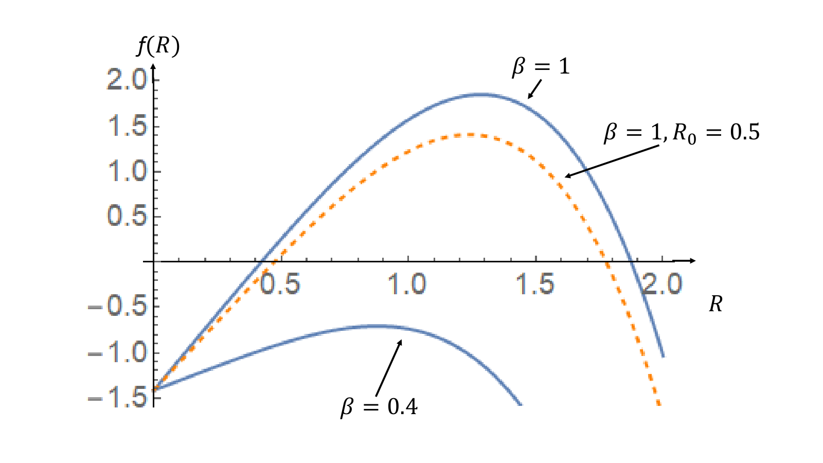
In Fig. 3 we plot the function $f(R)$ for two values of $\beta$; the graph shows the existence of two stationary radii, stable, $R_{+}(\beta)$ and unstable, $R_{-}(\beta)$, for $\beta=1$, while no stationary states for $\beta=0.4$. One can conclude that there exists a critical value $\beta_{c}$ such that there are no stationary solutions when $\beta<\beta_{c}$. Below we find that $\beta_{c}=0.637$ for the chosen set of parameters.

The critical value $\beta_{c}$ has to satisfy three constraints: (i) $MR_{0}^{3}+\Omega(\beta_{c})>0$, which guarantees the existence of maximum of $f(R)$ at a certain $R=R_{*}$, (ii) $f(R_{*},\beta_{c})=0$, (iii) $f^{\prime}_{R}(R_{*},\beta_{c})=0$ (see Fig. 4(b)). As a result we find that $\beta_{c}$ is the positive solution of the quadratic equation

$$MR_{0}^{3}+\Omega(\beta_{c})=2^{\frac{19}{8}}3^{\frac{-3}{4}}D^{\frac{3}{8}}M^{\frac{1}{4}},$$

(16)

that can be found explicitly:

	$\displaystyle\beta_{c}=\frac{1}{2S\Omega_{2}}\Bigg[A\Omega_{1}-$
	$\displaystyle\sqrt{(A\Omega_{1})^{2}-S\Omega_{2}\left(2^{\frac{27}{8}}3^{\frac{-7}{4}}D^{\frac{3}{8}}M^{\frac{1}{4}}-\frac{2}{3}MR_{0}^{3}\right)}\Bigg]$

For $\beta=\beta_{c}$,

$$R_{-}(\beta_{c})=R_{+}(\beta_{c})=R_{*}=2^{\frac{1}{8}}3^{\frac{-1}{4}}D^{\frac{1}{8}}M^{\frac{-1}{4}};$$

notice that $R_{*}$ does not depend on $R_{0}$; for values of parameters indicated in Fig. 2, $R_{*}=1.041$ . Because $\Omega(\beta)$ is a monotonically growing function of $\beta$, $R_{-}(\beta)$ decreases with the growth of $\beta$, and therefore $R_{-}(\beta)<R_{*}$ for any $\beta>\beta_{c}$. On the contrary, $R_{+}(\beta)$ increases with the growth of $\beta$. For values of parameters indicated in Fig. 2 and $R_{0}=1$, we find $\beta_{c}=0.637$ .

If $\beta<\beta_{c}$, then $f(R)<0$ for any $R$, therefore the cell radius decreases with time and tends to zero during a finite time (see Fig. 4(a)). The temporal evolution of $R(t)$ in the case of $\beta>\beta_{c}$ depends on the relation between the initial radius $R_{0}$ and $R_{-}(\beta)$. If $R_{0}>R_{-}(\beta)$, then $R(t)\to R_{+}(\beta)$ as $t\to\infty$; if $R_{0}<R_{-}(\beta)$, then $R(t)\to 0$ during a finite time. Therefore, if $R_{0}>R_{*}$, $R(t)$ tends to a finite value for any $\beta>\beta_{c}$, because $R_{-}(\beta)<R_{*}<R_{0}$. However, if $R_{0}<R_{*}$, the cell shrinks even at $\beta>\beta_{c}$, if $\beta$ is still less than a certain value $\tilde{\beta}$ (see Fig 4(c)), which is determined by the relation $R_{0}=R_{-}(\tilde{\beta})$ (see Fig. 4(d)). Because $f(R_{0},\tilde{\beta})=0$, the value of $\tilde{\beta}$ can be found by solving the equation,

$$\Omega(\tilde{\beta})=\frac{\sqrt{2D_{u}}}{R_{0}}.$$

For $\beta>\tilde{\beta}$, $R_{-}(\beta)<R_{0}$, therefore the cell radius tends to a finite value (see Fig. 4(e)).

In Fig. 5 we present the numerical solution of the ODE (15a) for the values $\beta=1$ . As we can see, the cell radius can increase monotonically until it reaches the steady state value. This is because in the framework of our model, the volume is not conserved and influences the dynamics through the parameter $\delta(r,t)$, see equation (5b).

The decrease of the cell radius (in the language of the phase-field model, the transition of the phase $u=1$ into the phase $u=0$) is caused by negative terms in the right-hand side of (1a),(3a), among them the term $-\delta(1-u)u$, which is negative at large $R$, and by the diffusion term, which creates an effective “surface tension” of the cell surface. The positive term $-\alpha u_{r}p$ hinders the decrease of the cell radius. If $\beta$ is not sufficiently large, the polarization is not strong enough to stop the collapse of the cell. In that case, the cell shrinks until it disappears (see Fig. 3, $\beta=0.4$.)

Note that at large $\beta$ (see Fig. 4(e)) we have $\Omega(\beta)\gg 1$, and $R_{-}(\beta)\ll 1$, therefore one can approximate the expression of $f(R)$ in (12) as:

$$R_{-}(\beta)\approx\frac{\sqrt{2D_{u}}}{\Omega(\beta)}.$$

We can see that for sufficiently large $\beta$, $R_{-}(\beta)$ can be arbitrary small. Therefore, for arbitrary small $R_{0}$, there exists such $\tilde{\beta}$ that the cell radius tends to a finite value, if $\beta>\tilde{\beta}$.

For values of parameters indicated in Fig. 2 and $R_{0}=0.5$, $\tilde{\beta}=0.96$ . In Fig. 3 and 5, we show the numerical plots for the parameters $\beta=1$, and $R_{0}=0.5$.

Let us emphasize that the described effect is not physical: for such values of parameters, the model does not reflect the true behavior of cells.

We employ the scaling and definitions of the previous section. Now we have to consider the azimuthal dependence of variable. One can calculate,

	$\displaystyle\partial_{\theta}=-\epsilon^{-1}R_{\theta}\partial_{\zeta}+\partial_{\theta},\ \partial_{\varphi}=-\epsilon^{-1}R_{\varphi}\partial_{\zeta}+\partial_{\varphi},$
	$\displaystyle\partial_{\theta}^{2}=\epsilon^{-2}R_{\theta}^{2}\partial_{\zeta}^{2}-\epsilon^{-1}(R_{\theta\theta}\partial_{\zeta}+2R_{\theta}\partial_{\zeta\theta}^{2})+\partial_{\theta}^{2},$
	$\displaystyle\partial_{\varphi}^{2}=\epsilon^{-2}R_{\varphi}^{2}\partial_{\zeta}^{2}-\epsilon^{-1}(R_{\varphi\varphi}\partial_{\zeta}+2R_{\varphi}\partial_{\zeta\varphi}^{2})+\partial_{\varphi}^{2},$
	$\displaystyle\frac{1}{r}\partial_{\theta}=-\frac{R_{\theta}}{R}\partial_{\zeta}+O(\epsilon),\quad\frac{1}{r^{2}}\partial_{\theta}=-\epsilon\frac{R_{\theta}}{R^{2}}\partial_{\zeta}+O(\epsilon^{2}),$
	$\displaystyle\frac{1}{r}\partial_{\varphi}=-\frac{R_{\varphi}}{R}\partial_{\zeta}+O(\epsilon),\quad\frac{1}{r^{2}}\partial_{\varphi}=-\epsilon\frac{R_{\varphi}}{R^{2}}\partial_{\zeta}+O(\epsilon^{2}),$
	$\displaystyle\nabla^{2}u=\left(1+\frac{R_{\theta}^{2}}{R^{2}}+\frac{R_{\varphi}^{2}}{R^{2}\cos^{2}\theta}\right)u_{\zeta\zeta}+$
	$\displaystyle\epsilon\Bigg[\left(\frac{2}{R}+\frac{R_{\theta}}{R^{2}}\tan\theta-\frac{R_{\theta\theta}}{R^{2}}-\frac{R_{\varphi\varphi}}{R^{2}\cos^{2}\theta}\right)u_{\zeta}$
	$\displaystyle-\frac{2}{R^{2}}\left(R_{\theta}u_{\zeta\theta}+\frac{R_{\varphi}}{\cos^{2}\theta}u_{\zeta\varphi}\right)$
	$\displaystyle-\frac{2\zeta}{R^{3}}\left(R_{\theta}^{2}+\frac{R_{\varphi}^{2}}{\cos^{2}\theta}\right)u_{\zeta\zeta}\Bigg]+O(\epsilon^{2}).$

The nonlocality in (1b) is approximated as follows,

$$\int u\textrm{d}^{3}r\sim\frac{\epsilon^{-3}}{3}\int_{0}^{2\pi}\textrm{d}\varphi\int_{-\pi/2}^{\pi/2}R^{3}(\theta,\varphi,t)\cos\theta\textrm{d}\theta.$$

We use expansions (7),and define the auxiliary function $\Lambda$,

$$\Lambda(\theta,\varphi,t)=\left(1+\frac{R_{\theta}^{2}}{R^{2}}+\frac{R_{\varphi}^{2}}{R^{2}\cos^{2}\theta}\right)^{-1/2}.$$

At the leading order one can fined,

	$\displaystyle D_{u}\Lambda^{-2}u_{0\zeta\zeta}=(1-u_{0})(\frac{1}{2}-u_{0})u_{0},$
	$\displaystyle D_{p}\Lambda^{-2}p_{0\zeta\zeta}-\tau^{-1}p_{0}=\beta u_{0\zeta},$
	$\displaystyle D_{p}\Lambda^{-2}q_{0\zeta\zeta}-\tau^{-1}q_{0}=-\beta\frac{R_{\theta}}{R}u_{0\zeta},$
	$\displaystyle D_{p}\Lambda^{-2}w_{0\zeta\zeta}-\tau^{-1}w_{0}=-\beta\frac{R_{\varphi}}{R\cos\theta}u_{0\zeta},$

therefore similarly to the previous section one can calculate the solutions

	$\displaystyle u_{0}(\zeta)=\frac{1}{2}\left[1-\tanh\left(\frac{\Lambda\zeta}{\sqrt{8D_{u}}}\right)\right],$		(17a)
	$\displaystyle p_{0}(\zeta)=\beta\Lambda\Phi(\Lambda\zeta)$		(17b)
	$\displaystyle q_{0}(\zeta)=-\beta\Lambda\frac{R_{\theta}}{R}\Phi(\Lambda\zeta)$		(17c)
	$\displaystyle w_{0}(\zeta)=-\beta\Lambda\frac{R_{\varphi}}{R\cos\theta}\Phi(\Lambda\zeta)$		(17d)

The equation for $u$ at the order $O(\epsilon)$ have the form,

	$\displaystyle D_{u}\Lambda^{-2}u_{1\zeta\zeta}-\left(\frac{1}{2}-3u_{0}+3u_{0}^{2}\right)u_{1}=-R_{t}u_{0\zeta}+$
	$\displaystyle-D_{u}\Bigg[\left(\frac{2}{R}+\frac{R_{\theta}}{R^{2}}\tan\theta-\frac{R_{\theta\theta}}{R^{2}}-\frac{R_{\varphi\varphi}}{R^{2}\cos^{2}\theta}\right)u_{0\zeta}$
	$\displaystyle-\frac{2}{R^{2}}\left(R_{\theta}u_{0\zeta\theta}+\frac{R_{\varphi}}{\cos^{2}\theta}u_{0\zeta\varphi}\right)$
	$\displaystyle-\frac{2\zeta}{R^{3}}\left(R_{\theta}^{2}+\frac{R_{\varphi}^{2}}{\cos^{2}\theta}\right)u_{0\zeta\zeta}\Bigg]$		(18)
	$\displaystyle+Au_{0\zeta}\left(p_{0}-\frac{R_{\theta}}{R}q_{0}-\frac{R_{\varphi}}{R\cos\theta}w_{0}\right)+$
	$\displaystyle(1-u_{0})u_{0}\left\{\tilde{V}(t)-S(p_{0}^{2}+q_{0}^{2}+w_{0}^{2})\right\},$

where the volume variation has the form,

$$\tilde{V}(t)=M\left[\frac{1}{4\pi}\int_{0}^{2\pi}\textrm{d}\varphi\int_{-\pi/2}^{\pi/2}R^{3}(\theta,\varphi,t)\cos\theta\textrm{d}\theta-R_{0}^{3}\right].$$

We apply the solvability condition, which is the orthogonality of the equation’s right-hand side to the solution of the homogenous equation $u_{0\zeta}$, and obtain a closed form of the interface dynamics,

$$a\Lambda R_{t}=-2aD_{u}\mathcal{H}-\tilde{V}+\Omega,$$

(19)

where

$$\mathcal{H}=\frac{1}{2}\nabla\cdot\hat{n}=\frac{1}{2}\nabla\cdot\left(\frac{\nabla(r-R)}{|\nabla(r-R)|}\right)$$

(20)

is the mean local curvature of the surface $r=R(\theta,\varphi,t)$. For an explicit expression of the curvature see Appendix A. Note that in the spherically symmetric case $\Lambda=1$, $H=1/R$ and $\tilde{V}=M[R^{3}(t)-R_{0}^{3}]$. Therefore, equation (12) is recovered from equation (19). Notice that $\Omega$ in equation (19), depends on all of the parameters that describe the nonequilibrium molecular effects of the subcell level, see (13), and (14). Equation (19) is a closed evolutionary equation for the 3D cell interface dynamics , which is an integro-differential equation, i.e., it is nonlocal, unlike that obtained in the spherical case (15a). For the details of the application of the solvability condition in order to obtain equation (19), we refer the reader to Hamed and Nepomnyashchya 2020 and Hamed and Nepomnyashchya 2016, where we perform similar calculations.

Notice that in (19) the expression $\Lambda R_{t}$ corresponds to the normal velocity $v_{n}$ of the interface, thus that equation is a generalization of the well-known curvature flow. By a proper scaling transformation, $t\rightarrow a^{2}t$ and $R(t)\rightarrow aR(t)$, the equation of motion of the cell boundary can be brought to a canonical form,

$$v_{n}=-2D_{u}\mathcal{H}-\tilde{V}+\Omega.$$

In addition it suggests an answer for the unrevealed force – velocity relation for the actin network that was highlighted in Keren et al. 2008 in the context of shape dynamics of a 2D cell.

We perform the analysis of a minimal phase field model that is a 3D generalization of the 2D model developed and investigated numerically in Ziebert et al. 2012, Ziebert and Aranson 2014, and Ziebert and Aranson 2016 (a similar analysis of the latter model was done in Hamed and Nepomnyashchya 2020). In this model the order parameter $u$ is coupled with 3D polarization (orientation) vector field P of the actin network. The model is supposed to describe the 3D cell motility immersed in 3D ECM via actin based protrusion mechanism Caswell and Zech 2018.

We considered the rotational symmetric case i.e., spherical shape interface, where we obtained a closed ordinary differential equation describing the evolution of the radius (15a). We found the minimum value $\beta_{c}$ for the actin creation that is compatible with the existence of a stationary cell solution (16). We found that when $\beta_{c}<\beta$, the circular cell can have some stationary radius, while in the case $\beta\leq\beta_{c}$ the cell shrinks until it disappears, which is meaningless in the context of cell dynamics. Also, we considered the general shape 3D cell dynamics. We found the leading order solutions, (17a)-(17c), and derived a closed integro-differential equation (19) governing the 3D cell dynamics, which includes the normal velocity of the membrane, curvature, volume relaxation rate, and a parameter $\Omega$ determined by the molecular effects of the subcell level. This result is similar to the 2D case Hamed and Nepomnyashchya 2020.

We found an equation of motion of the cell interface that can be written in the canonical form,

$$v_{n}=-2D_{u}\mathcal{H}-\tilde{V}+\Omega.$$

The stability analysis shows that the non-spherical shape and the motion of the cell as a whole cannot appear due to the development of a linear instability of the spherical cell with the spherically symmetric polarization field localized near the cell boundary. In the framework of the considered model, the transition to a non-spherical shape needs a finite-amplitude disturbance significantly changing the polarization field inside the cell. The analysis of that transition, which can be carried out only numerically, is beyond the scope of the present paper.

References

- Ziebert et al. (2012) F. Ziebert, S. Swaminathan, and I. S. Aranson, “Model for self-polarization and motility of keratocyte fragments,” J. R. Soc. Interface 9, 1084–1092 (2012).
- Hamed and Nepomnyashchya (2020) M. Abu Hamed and A.A. Nepomnyashchya, “A simple model of keratocyte membrane dynamics: The case of motionless living cell,” Physica D 408 (2020).
- Tjhung et al. (2015) E. Tjhung, A. Tiribocchi, D. Marenduzzo, and M.E. Cates, “A minimal physical model captures the shapes of crawling cells,” Nature Communications 6:5420 (2015).
- Mai and Camley (2020) M. H. Mai and B. A. Camley, “Hydrodynamic effects on the motility of crawling eukaryotic cells,” Soft Matter 16 (2020).
- Zaman et al. (2005) M. H. Zaman, R. D. Kamm, P. Matsudaira, and D. A. Lauffenburger, “Computational model for cell migration in three-dimensional matrices,” Biophysical Journal 89, 1389–1397 (2005).
- Schlüter et al. (2012) D. K. Schlüter, I. R. Conde, and M. A. J. Chaplain, “Computational modeling of single-cell migration: The leading role of extracellular matrix fibers,” Biophysical Journal 103, 1141–1151 (2012).
- Wu et al. (2018) P. Hsun Wu, D. M. Gilkes, and D. Wirtz, “Annual review of biophysics: The biophysics of 3d cell migration,” Annu. Rev. Biophys. 47, 549–67 (2018).
- Mogilner (2008) A. Mogilner, “Mathematics of cell motility: have we got its number?” Mathematical Biology 58, 105–134 (2008).
- Mogilner et al. (2020) A. Mogilner, E. L. Barnhart, and K. Keren, “Experiment, theory, and the keratocyte: An ode to a simple model for cell motility,” Seminars in Cell and Developmental Biology 100, 143–151 (2020).
- Keren et al. (2008) K. Keren, Z. Pincus, G. M. Allen, E. L. Barnhart, G. Marriott, Alex Mogilner, and J. A. Theriot, “Mechanism of shape determination in motile cells,” nature 453 (2008).
- Caswell and Zech (2018) P. T. Caswell and T. Zech, “Actin-based cell protrusion in a 3d matrix,” Trends in Cell Biology 28 (2018).
- Winkler et al. (2019) B. Winkler, I. S. Aranson, and F. Ziebert, “Confinement and substrate topography control cell migration in a 3d computational model,” Communications Physics 2:82 (2019).
- Ziebert and Aranson (2014) F. Ziebert and I. S. Aranson, “Modular approach for modeling cell motility,” Eur. Phys. J. Special Topics 223, 1265–1277 (2014).
- Ziebert and Aranson (2016) F. Ziebert and I. S. Aranson, “Computational approaches to substrate-based cell motility,” npj Computational Materials 6 (2016).
- Hamed and Nepomnyashchya (2016) M. Abu Hamed and A.A. Nepomnyashchya, “Dynamics of curved fronts in systems with power-law memory,” Physica D 328-329, 1–8 (2016).