Evidence for a Cloud-Cloud Collision in Sh2-233 Triggering the Formation of the High-mass Protostar Object IRAS 05358+35432015Evidence for a Cloud-Cloud Collision in Sh2-233 Triggering the Formation of the High-mass Protostar Object IRAS 05358+3543–11

Rin I. Yamada Yasuo Fukui Thanks: E-mail: yamada@a.phys.nagoya-u.ac.jp Affiliation: Department of Physics, Nagoya University, Furo-cho, Chikusa-ku, Nagoya 464-8601, Japan Hidetoshi Sano Affiliation: Institute for Advanced Research, Nagoya University, Furo-cho, Chikusa-ku, Nagoya 464-8601, Japan Kengo Tachihara Affiliation: National Astronomical Observatory of Japan, Mitaka, Tokyo 181-8588, Japan John H. Bieging Affiliation: Department of Physics, Nagoya University, Furo-cho, Chikusa-ku, Nagoya 464-8601, Japan Rei Enokiya Affiliation: Steward Observatory, The University of Arizona, Tucson, AZ 85721, USA Atsushi Nishimura Affiliation: Department of Physics, Faculty of Science and Technology, Keio University, 3-14-1 Hiyoshi, Kohoku-ku,Yokohama, Kanagawa 223-8522, Japan Shinij Fujita Affiliation: Institute of Astronomy, the University of Tokyo, 2-21-1 Osawa, Mitaka, Tokyo 181-0015, Japan Mikito Kohno Affiliation: Department of Physics, Nagoya University, Furo-cho, Chikusa-ku, Nagoya 464-8601, Japan Affiliation: Department of Physical Science, Graduate School of Science, Osaka Prefecture University, 1-1 Gakuen-cho, Naka-ku, Sakai 599-8531, Japan Affiliation: Astronomy Section, Nagoya City Science Museum, 2-17-1 Sakae, Naka-ku, Nagoya, Aichi, 460-0008, Japan Kisetsu Tsuge Affiliation: Department of Physics, Nagoya University, Furo-cho, Chikusa-ku, Nagoya 464-8601, Japan

Accepted XXX. Received YYY; in original form ZZZ

Abstract

We have carried out a new kinematical analysis of the molecular gas in the Sh2-233 region by using the CO $J$ = 2–1 data taken at $\sim$ 0.5 pc resolution. The molecular gas consists of a filamentary cloud of 5-pc length with 1.5-pc width where two dense cloud cores are embedded. The filament lies between two clouds, which have a velocity difference of 2.6 km s^-1 and are extended over $\sim$ 5 pc. We frame a scenario that the two clouds are colliding with each other and compressed the gas between them to form the filament in $\sim$ 0.5 Myr which is perpendicular to the collision. It is likely that the collision formed not only the filamentary cloud but also the two dense cores. One of the dense cores is associated with the high-mass protostellar candidate IRAS 05358+3543, a representative high-mass protostar. In the monolithic collapse scheme of high mass star formation, a compact dense core of 100 $M_{\odot}$ within a volume of 0.1 pc radius is assumed as the initial condition, whereas the formation of such a core remained unexplained in the previous works. We argue that the proposed collision is a step which efficiently collects the gas of 100 $M_{\odot}$ into 0.1 pc radius. This lends support for that the cloud-cloud collision is an essential process in forming the compact high-mass dense core, IRAS 05358+3543.

Keywords:

stars: formation – ISM: clouds – ISM: individual objects: IRAS 05358+3543

1 Introduction

High-mass star formation is an important process which substantially affects the galaxy evolution via enormous energy inputs into the interstellar medium (ISM). The energy inputs regulate the physical conditions of the ISM and control the gravitational collapse of the ISM which leads to high-mass star formation. The mechanism of high-mass star formation, however, has been an issue difficult to solve. The reason for this is multi-fold. The region of high-mass star formation is rare in the solar neighbourhood and detailed observations of this process were difficult as compared with the sites of low-mass star formation. Further, the timescale of high-mass star formation is probably very short, less than Myr, because of higher density of the star forming core, making a marked contrast with the low-mass star formation which proceeds slowly in 100 Myr due to low density. Because of this contrast, there is a high barrier in finding out the high-mass star formation location and to resolve the star formation process therein with sufficient details. In spite of such difficulties, progress has been achieved by extensive surveys for massive dense cores, and hundreds of such cores have been catalogued in the Galactic plane (e.g., Beuther et al. 2010; Urquhart et al. 2014). Massive dense cores are believed to be precursors of high-mass stars because a high mass protostar should experience a massive dense core phase prior to a mature high-mass star. It is however not certain if all the massive cores are actual sites of high-mass star formation, since most of them lack a Hii region, an unmistakable sign of high-mass stars emitting strong UV radiation. It was also puzzling that the number of such cores are large, suggesting a long timescale like 10 Myr, leaving room to suspect that many of the cores, even if not all, may not be such precursors but stay stable as they are.

The observational difficulties may be overcome by theoretical works. McKee & Tan 2003 investigated typical density inherent to the earliest phase of the high mass star formation in the literature, and found that many of the high mass star forming regions have common surface mass density around 1 g cm^-2, which corresponds to column density of $\sim 3\times 10^{23}$ cm^-2. Cases of the high-column density in high-mass star formation include the massive clusters, the Orion Nebula Cluster in M42 and W3 Main, where around ten O stars are formed (for reviews O’Dell et al. 2008 and Megeath et al. 2008), as well as a more isolated high-mass protostar IRAS 05358+3543 in Sh2-233 (Beuther et al. 2007; see for a review Reipurth & Yan 2008). Krumholz et al. 2009 made hydrodynamical numerical simulations of gravitational collapse of a massive cloud core under the assumed initial condition, 100 $M_{\odot}$ within 0.1 pc, corresponding to the condition found in the above regions. The simulations, which are usually referred to as the monolithic collapse models, successfully produced two $\sim$ 30 $M_{\odot}$ stars in binary in a timescale of a few times 10⁴ yr, and showed that the issue of high mass star formation may be solved by the model.

It however remained to be explained how such a massive dense core can be formed in the ISM. The fact that such massive dense cores can form high-mass stars rapidly without fail suggests that the core may rapidly collapse to lower-mass stars well before collected as a massive core. If one traces the whole gravitational collapse initiating by low density like 1000 cm^-3, the initial condition assumed by the monolithic collapse model might be hardly realised with self-gravity alone. This reasoning may be supported by the scenarios of a cloud-cloud collision in a number of star forming regions by the recent observational works including well known Hii regions M20, M42 and M17 (Torii et al. 2017; Fukui et al. 2018; Nishimura et al. 2018), giant molecular clouds with mini-starbursts W43, W51, and Carina (Kohno et al. 2021; Fujita et al. 2021a; Fujita et al. 2021b), the Galactic centre (Enokiya et al. 2021a; Tsuboi et al. 2021), the Magellanic Clouds (Fukui et al. 2017; Tsuge et al. 2019), M33 (Sano et al. 2021; Tokuda et al. 2020; Kondo et al. 2021), and the Antennae galaxies (Tsuge et al. 2021a; Tsuge et al. 2021b) as well as theoretical results of colliding molecular gas flows (Inoue & Fukui 2013; Inoue et al. 2018; Fukui et al. 2020a). See also Fukui et al. 2020b for a review of the related observational and theoretical works. Such colliding gas flows can significantly accelerate the gas collection by the supersonic motion, ten times faster than the free fall, without converting gas into stars, and may be a crucial step in forming a massive core.

In the present paper, we intend to make a detailed kinematic study of the gas in the region of Sh2-233IR at $\sim$ 10′ to the southeast of Sh2-233, one of the representative cases of high gas surface density including the high mass protostar candidate IRAS 05358+3543. The region harbours other Hii regions Sh2-231, Sh2-232, and Sh2-235 in addition to Sh2-233 (see for a review Reipurth & Yan 2008), which are located at a distance of 1.8 kpc (Evans & Blair 1981) and within 40 pc of Sh2-233 on its eastern side in the galactic coordinate. This is a relatively dense region of star formation along the Galactic plane. It may be considered that these Hii regions are expanding to accelerate the gas and triggering star formation in the surroundings according to a picture of Elmegreen & Lada 1977, because the Hii regions can agitate the surrounding gas to accelerate expanding motions in a timescale of several Myrs or more, the probable duration of these extended Hii regions. The active O star formation attracted attention and stimulated a number of works on star formation at multi-wavelength. Most recently, a detailed analysis of the CO gas in Sh2-235 were carried out by Dewangan & Ojha 2017 (see the references therein for observational works at multi-wavelength). This work suggests that a cloud cloud collision is a viable mechanism of a recent trigger of star formation within a timescale of Myr, whereas the acceleration of the gas clouds, which may be Hi or H₂ clouds, could have originated more than a few Myr ago by acceleration due to Hii regions.

The present work is organised as follows; Section 2 summarises the data used in the analysis and Section 3 the results of the analysis. Section 4 discusses the implications and Section 5 gives conclusions.

2 Datasets

We made use of the archival $J$ = 2–1 data of the ¹²CO and ¹³CO emission obtained with the Heinrich Hertz Submillimeter Telescope (SMT) at the Arizona Radio Observatory (Bieging et al. 2016). Entire observations were carried out by using the fully-sampled on-the-fly (OTF) method with a full half power beam width (HPBW) of 32 $″$ . The ¹²CO and ¹³CO data are both convolved to a spatial resolution of 38 $″$ . Both ¹²CO and ¹³CO data cubes were resampled onto identical velocity grids with 0.15 km s^-1 spacing by third-order interpolation. The typical noise fluctuations are 0.10 K for ¹²CO and 0.12 K for ¹³CO at 0.15 km s^-1 velocity grid. For more details of the observations, see Bieging et al. 2016.

3 Results

3.1 Gas distribution toward the Sh2-233 region

Refer to caption — Figure 1: Integrated intensity distribution of the ¹³CO( $J$ = 2–1) emission for a velocity range from $-22$ km s^-1 to $-12$ km s^-1. Contours are plotted every 6 K km s^-1 from 2 K km s^-1. Black crosses indicate the positions of Sh2-233, IRAS 05358+3543, and G173.58+2.45 corresponding to ( $\alpha_{\mathrm{J2000}}$ , $\delta_{\mathrm{J2000}}$ ) = ( $05^{\mathrm{h}}38^{\mathrm{m}}31.5^{\mathrm{s}}$ , $35$ °51′19″), ( $\alpha_{\mathrm{J2000}}$ , $\delta_{\mathrm{J2000}}$ ) = ( $05^{\mathrm{h}}39^{\mathrm{m}}10.4^{\mathrm{s}}$ , $35$ °45′19″), ( $\alpha_{\mathrm{J2000}}$ , and $\delta_{\mathrm{J2000}}$ ) = ( $05^{\mathrm{h}}39^{\mathrm{m}}27.7^{\mathrm{s}}$ , $35$ °40′43″), respectively. White crosses show the positions of YSOs detected by Marton et al. 2016. Black rectangle outlines the region for which we obtained masses in section 3

The molecular gas in the Sh2-233 region has velocity in a range from $-22$ km s^-1 to $-12$ km s^-1. Figure 1 shows the total integrated intensity of ¹³CO( $J$ = 2–1) in the velocity range. Hereafter, we shall use mostly ¹³CO( $J$ = 2–1) which is optically thin and suited for tracing gas density. The molecular gas in the region shows filamentary distribution (hereafter “filament”) extending from the southeast to the northwest. Toward the brightest ¹³CO( $J$ = 2–1) peak at ( $\alpha_{\mathrm{J2000}}$ , $\delta_{\mathrm{J2000}}$ ) $\sim$ ( $05^{\mathrm{h}}39^{\mathrm{m}}12^{\mathrm{s}}$ , $35$ °45′40″), the high-mass protostar candidate IRAS 05358+3543 shown by a black cross and a few additional YSOs are located as shown by the white crosses (Marton et al. 2016). Another peak corresponding to G173.58+2.45 is located in the southeast at ( $\alpha_{\mathrm{J2000}}$ , $\delta_{\mathrm{J2000}}$ ) $\sim$ ( $05^{\mathrm{h}}39^{\mathrm{m}}30^{\mathrm{s}}$ , $35$ °40′) and the third one at the northwest ( $\alpha_{\mathrm{J2000}}$ , $\delta_{\mathrm{J2000}}$ ) $\sim$ ( $05^{\mathrm{h}}38^{\mathrm{m}}45^{\mathrm{s}}$ , $35$ °40′).

Figure 2 shows velocity channel distributions of ¹³CO( $J$ = 2–1) ranging from $-21.5$ km s^-1 to $-13.4$ km s^-1 every 0.9 km s^-1. Many panels show the filament with local peaks as substructures. The Panels (a) to (e) show the blue-shifted component and the panel (g) to (i) show red-shifted component.

Figure 3a shows the first moment of ¹³CO( $J$ = 2–1) where integrated intensity >10 K km s^-1 is uniform at about $-16$ km s^-1 in the southwest, and that is uniform at around $-18$ km s^-1 in the northeast. We find that there is a velocity difference of $\sim$ 2.6 km s^-1 between the southwestern and northeastern components within $\sim$ 5′ of the filament. Figure 3b shows the second moment of ¹³CO( $J$ = 2–1), which is enhanced by a factor of 2–4 from 0.6 km s^-1 to 1.6 km s^-1 toward the filament with a width of 1–2 pc. It seems that the red-shifted component is somewhat more localised in the $\alpha_{\mathrm{J2000}}$ from $05^{\mathrm{h}}38^{\mathrm{m}}30^{\mathrm{s}}$ to $05^{\mathrm{h}}39^{\mathrm{m}}20^{\mathrm{s}}$ in panels (h) and (i) of Figure 2 and Figure 3a.

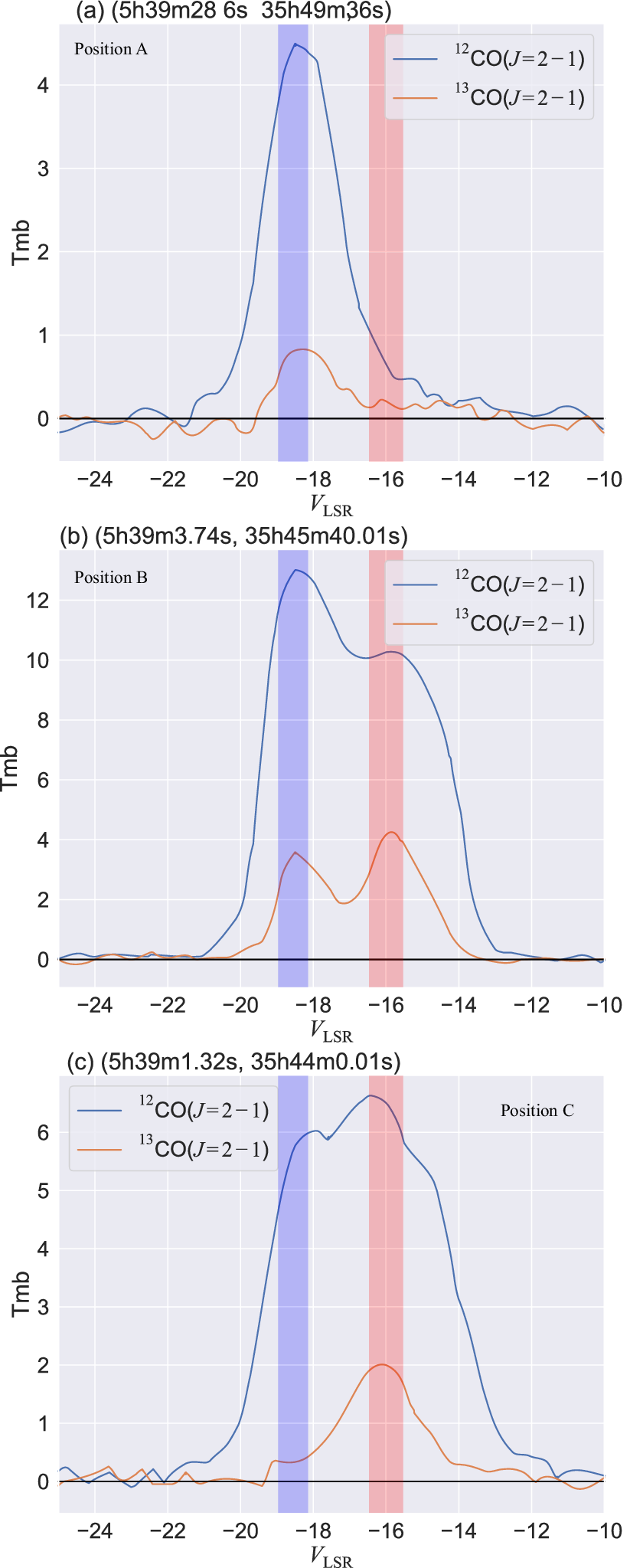
Figure 4 shows typical CO profiles near Sh2-233IR in the three positions in Figure 3a (A), (B), and (C). Figures 4a and 4c show single peaks which are blue-shifted in (a) and red-shifted in (c) and the peak velocity coincides with the first moment in Figure 3a , and Figure 4b shows a double peak (B) in both ¹²CO( $J$ = 2–1) and ¹³CO( $J$ = 2–1). Considering all of the above, we interpret that gas in the region of Sh2-233 consists of two different velocities toward the filament. We hereafter call the red-shifted component red cloud and the blue-shifted component blue cloud.

3.2 The red- and blue-shifted clouds

We now consider the properties of the red and blue-shifted clouds in Sh2-233. Following Enokiya et al. 2021b who analysed two molecular clouds in the NGC 2024 region, we use a method based on the first moment and the second moment to define representative velocity ranges of the two clouds. First, we assume that the two clouds are overlapping toward the intermediate region with non-overlapping outside the region. This means that the northeastern and the southwestern regions outside the filament are non-overlapping regions. The concrete procedure is described as follows;

1.

We exclude the region with second moment higher than 1.5 km s^-1 as the overlapping region (Figure 3).
2.

We define the regions of the red and blue clouds as the first moment $>-17$ km s^-1 and $<-17$ km s^-1, respectively.
3.

We average the first and second moments within the defined areas.

From Figure 3b and Figure 4, the typical spectra at the region with second moment >1.5 km s^-1 have either two peaks, or are merged into a single peak. We see a dip at a typical velocity of $\sim$ $-17$ km s^-1. These suggest that the second moment >1.5 km s^-1 and the the first moment $>-17$ km s^-1 and $<-17$ km s^-1 criteria give suitable representatives for the red and blue clouds.

The velocity range for the red cloud is defined as from $V_{\mathrm{representative,red}}$ - $dV_{\mathrm{red}}$ to $V_{\mathrm{representative,red}}$ + $dV_{\mathrm{red}}$ and the velocity range for the blue cloud as from $V_{\mathrm{representative,blue}}$ - $dV_{\mathrm{blue}}$ to $V_{\mathrm{representative,blue}}$ + $dV_{\mathrm{blue}}$ where $V_{\mathrm{representative,red}}$ , $V_{\mathrm{representative,blue}}$ , $dV_{\mathrm{red}}$ , $dV_{\mathrm{blue}}$ are $-16.00$ km s^-1, $-18.55$ km s^-1, $0.48$ km s^-1, $0.40$ km s^-1, respectively.

By applying these criteria we derived the representative velocity range of the blue cloud to be $-19.0$ km s^-1 to $-18.2$ km s^-1, and that of the red cloud to be $-16.5$ to $-15.5$ km s^-1. Figure 5 shows the distributions of the red and blue clouds, and the two clouds are both peaked toward IRAS 05358+3543. Figure 6 shows an overlay of the two clouds, confirming that the filamentary distribution coincides with the area where the two clouds are overlapping. We also find that the blue cloud has a sharp intensity drop to the southwest and is extended to the northeast with another filamentary feature extending to the north from the IRAS 05358+3543 core. In contrast to the blue cloud, the red cloud is extended to the southeast with a relatively sharp drop toward the northeast.

3.3 The physical properties of the clouds

By assuming the local thermodynamical equilibrium we derived the column density of the molecular gas. For the area of the two clouds in section 3.2. for a range from $-22$ km s^-1 to $-12$ km s^-1. By assuming that the ¹²CO( $J$ = 2–1) line is optically thick we estimated $T_{\mathrm{rms}}$ in each pixel. Then the ¹³CO( $J$ = 2–1) optical depth was calculated from the radiation transfer equation and the ¹³CO column density. The ratio of H₂ to ¹³CO is assumed to be $5.0\times 10^{5}$ (Dickman 1978). The results are given in Tab. 1. We note that the masses of the red and blue clouds include the mass of the filament. For more details, see Appendix.

3.4 The molecular outflows associated with IRAS 05358+3543 and G173.58+2.45

Two molecular outflows were detected in the ¹²CO( $J$ = 1–0) emission toward IRAS 05358+3543 and G173.58+2.45 by Snell et al. 1990 and Shepherd & Churchwell 1996, respectively. Figures 8 and 9 show their spatial distributions of the ¹²CO( $J$ = 2–1) and ¹³CO( $J$ = 2–1) outflow wings and typical profiles in the present data. The velocity ranges and the other physical parameters including size, outflow velocity, mass, dynamical time scale, mass loss rate, and outflow momentum are calculated for a detection limit of 5 $\times T_{\mathrm{rms}}$ under an assumption of intensity ratio of the ¹²CO( $J$ = 2–1)/¹²CO( $J$ = 1–0) of 0.8 by referring to the ¹²CO( $J$ = 1–0) emission (Shepherd & Churchwell 1996) where the same as assumed in IRAS 05358+3543. The $X_{\mathrm{CO}}$ factor is assumed to be 1.0 $\times$ 10²⁰ [K km s^-1 cm^-2] (Okamoto et al. 2017) for the two objects. The results listed in Tab. 2 are basically consistent with the previous observations, while the size of the IRAS 05358+3543 outflow was found to be a factor of about two smaller than that in Snell et al. 1990. This could be due to the higher resolution of the present data 38″ than that by Snell et al. 1990, who adopted a grid spacing of 1–1.5′ with a 45″ beam.

Table 1: Physical parameters of the molecular clouds

Cloud name	Column density	Mass
	(cm^-2)	( $M_{\odot}$ )
(1)	(2)	(3)
Filament	$2.2\times 10^{22}$	$1030$
Red cloud	$1.3\times 10^{22}$	$580$
Blue cloud	$1.9\times 10^{22}$	$1630$

Notes. – Col.(1) Cloud name. Col.(2) The peak column density of each cloud/filament. Col.(3) Masses derived by assuming the local thermodynamical equilibrium in $\alpha_{\mathrm{J2000}}$ and $\delta_{\mathrm{J2000}}$ ranges of $05^{\mathrm{h}}38^{\mathrm{m}}31^{\mathrm{s}}$ – $05^{\mathrm{h}}39^{\mathrm{m}}12^{\mathrm{s}}$ and $35$ °37′30″– $35$ °51′46″, respectively. For the filament, we used the region enclosed by a third-lowest contour corresponding to 14 K km s^-1 in Fig. 1. For the red/blue cloud, The mass is derived by the region where the first moment is larger/smaller than -17 km s^-1 and the second moment is smaller than 1.5 km s^-1 in a velocity range from $-22$ km s^-1 to $-12$ km s^-1 in Fig. 3. For more details of the method, see Enokiya et al. 2021b. Note that we only use voxels with intensity higher than 5 $\times T_{\mathrm{rms}}=0.6$ K in Col.(2)–(3).

Table 2: Physical parameters of the molecular outflows

Lobe name	Size	$V_{\mathrm{sys}}$	$V_{\mathrm{outflow}}$	Mass	$t_{\mathrm{dyn}}$	Mass loss rate	Momentum
	(pc)	(km s^-1)	(km s^-1)	( $M_{\odot}$ )	(Myr)	( $M_{\odot}$ yr^-1)	(km s^-1 $M_{\odot}$ )
(1)	(2)	(3)	(4)	(5)	(6)	(7)	(8)
IRAS 05358+3543 blue lobe	$0.73$	$-16.1$	$12.3$	$44$	$0.14$	$3.1\times 10^{-4}$	$541$
IRAS 05358+3543 red lobe	$0.56$	$-16.1$	$10.5$	$28$	$0.12$	$2.3\times 10^{-4}$	$294$
G173.58+2.45 blue lobe	$0.71$	$-16.7$	$12.9$	$53$	$0.13$	$4.0\times 10^{-4}$	$683$
G173.58+2.45 red lobe	$0.98$	$-16.7$	$10.8$	$48$	$0.23$	$2.0\times 10^{-4}$	$518$

Notes. — Col. (1) Lobe name. Col. (2) Effective diameters defined by ( $A$ / $\pi$ ) ${}^{1/2}\times$ 0.5, where $A$ is the region enclosed by the lowest contours in Figs. 8a and 9a. Col. (3) Systemic velocities defined as peak velocities of ¹³CO( $J$ = 2–1). Col. (4) Three-sigma level maximum radial velocity of the outflow lobe with respect to the systemic velocity. Col. (5) Masses of the lobes. Col. (6) Dynamical time scale derived by dividing the two most distant points on the lowest contour by $V_{\mathrm{outflow}}$ Col. (7) Mass loss rate derived by Mass/ $t_{\mathrm{dyn}}$ . Col. (8) Momentum estimated by Mass $\times V_{\mathrm{outflow}}$ .

4 Discussion

4.1 Triggered star formation in the Sh2-233 region

The present Sh2-233 region is located relatively far from the other Hii regions including Sh2-235, and the present results show that the molecular gas in the region consists of two clouds at different velocities. It is possible that the two clouds, having complementary distribution (Fig. 6), are colliding with each other. If we assume that the collision took place in the northeast to the southwest direction, it is likely that the collision compressed the gas to form the filamentary clouds between them. It is also probable that the formation of the filament accompanied the formation of the dense cores in the filament as suggested by the magnetohydrodynamical numerical simulations of colliding molecular flows (Inoue & Fukui 2013).

Another piece of evidence for colliding clouds is found in the position velocity diagram in Figure 7, indicating a velocity jump of two clouds which are connected with each other. This distribution is understood as caused by collisional merging, where the intermediate velocity gas is caused in the interface layer where gas is mixed in velocity between the two clouds. Figure 7f shows that there are weak ¹³CO( $J$ = 2–1) emissions outside of a velocity range of $-21$ km s^-1 to $-12$ km s^-1 localised toward X-OFFSET=0. These weak emissions are possibly ascribed to part of the outflow wings (Figure 8), whereas it is not likely that the weak ¹³CO( $J$ = 2–1) outflow wings significantly alter the velocity jump.

We find that the blue cloud shows asymmetry relative to the filamentary cloud in the sense that the gas is extended to the northeast, while there is little gas distributed in the southwest. It is possible that the gas is more extended to the southwest of the blue cloud. The asymmetry is explained as due to sweeping up of the initially extended gas distribution by the red cloud, the compressed gas column density amounts to 2.2 $\times$ 10²² cm^-2. A similar, less pronounced asymmetry in the opposite sense is found in the red cloud that has extended gas in the southwest of the filament, which may be explained by a similar sweeping up on the opposite side. It is possible that the low density gas in the two clouds was compressed and enhanced as the filamentary cloud within $\sim$ 1 Myr, the collision time scale as shown below. So, the large-scale gas distribution at $\sim$ 5 pc seems also to be consistent with the collision picture.

The data available allow us to construct a detailed collisional picture of the formation of the cloud and stars. We frame a scenario of a cloud-cloud collision as follows; the blue cloud in the northeast collided with the red cloud about $\sim$ 6 $\times$ 10⁵ yr ago (=1.5 pc/2.5 km s^-1) by assuming that the angle between the collision velocity vector and the line of sight is 45 deg. The timescale varies depending on the assumed angle from 5 $\times$ 10⁵ yr to 8 $\times$ 10⁵ yr for a range of angle from 30 deg. to 60 deg. The main range of the collision is from 38^m50^s to 39^m40^s in RA and from 35°38′to 39°48′in Dec. The collision between the two clouds compressed the interface layer to form the filamentary cloud over $\sim$ 5 pc in the direction perpendicular to the collision direction. It seems the collision produced at least the two cores toward Sh2-233IR and G173.58+2.45 nearly synchronously.

4.2 The two regions of recent star formation triggered by the cloud-cloud collision

The most active star formation is taking place in the core toward Sh2-233IR where IRAS 05358+3543 is located. The core has a radius of 0.4 pc and its mass is estimated to be 230 $M_{\odot}$ . For details, see Appendix. Porras et al. 2000 made JHK photometric observations of Sh2-233IR and identified two clusters NE and SW, which are separated with each other by 0.5 pc in the direction perpendicular to the filament. The NE cluster on the filament is significantly redder than the SE cluster, which is more exposed and shifted to the southwest from the filament. IRAS 05358+3543 is most likely a member of the cluster NE and the associated outflow has a dynamical age of $\sim$ 10⁴ yr. This dynamical age is shorter than the collisional time scale of (5-8)×105 yr, which is consistent with the numerical simulations of colliding clouds (Fukui et al. 2020a), and does not contradict the stellar age upper limit, 2 Myr.

A question arising is if the formation of the cluster is due to the gravitational instability in the filamentary cloud and the gas flow along the filament collects the mass into the cluster. We suggest that the cluster formation is more strongly influenced by the initial density distribution prior to the filament formation than the flow along the filament, and dominated by the dynamical compression in the collision. This is because the column density of the blue cloud is enhanced in the northeast of the Sh2-233IR and by the collision the enhanced density will increase the core mass more rapidly than in the rest of the filament. Figure 10 shows two strips along and perpendicular to the filament including the two cores and clearly shows that the column density is enhanced at X-OFFSET=0.0. We suggest that the enhancement of the blue cloud in column density as indicated by the cloud extended to the north favoured the formation of the Sh2-233IR core, and thereby the formation of IRAS 05358+3543. At an even smaller sub-pc scale Sh2-233IR has sub-mm/mm clumps resolved into several dust condensations mm1a-b, mm2a-d, mm3, several of which have protostellar nature Larionov et al. 1999; Beuther et al. 2002; Beuther et al. 2007; Leurini et al. 2007 and one of them, mm1a is likely associated with the 1.3 mm continuum emission, which is extended in the same direction with the filament at a $\sim$ 1′ scale. This elongation may be indicate the effect of the collision.

The G173.58+2.45 core is associated with IRAS 05361+3539 and an ultra-compact Hii region. CO outflow is driven by a late B or mid A star (Shepherd & Churchwell 1996) in a small cluster of Class I and II sources (Chakraborty et al. 2000; Shepherd & Watson 2002; Varricatt et al. 2005), H₂O masers (Wouterloot & Brand 1989; Palagi et al. 1993), and H₂ emission shocks (Chakraborty et al. 2000; Varricatt et al. 2005).

Another core is toward the Hii region Sh2-233 having a B1 star (Hunter and Massey 1990) with an age of 10⁵ yr and is associated with IRAS source (IRAS05351+3549) (Casoli et al. 1986; Wouterloot & Brand 1989) and no masers (Wouterloot & Brand 1989; Wouterloot et al. 1993; Bronfman et al. 1996). Jiang et al. 2000 reported outflow toward the source, but no CO wing profile was shown. The core has loose connection to the present collision and requires to be confirmed.

The column densities toward the two cores are (1-2) $\times 10^{22}$ cm^-2 at several times 0.1 pc, and they are forming at least a single high-mass star in each core. This is consistent with the statistics of other $\sim$ 50 cloud-cloud collision objects compiled by Enokiya et al. 2021a and Fukui et al. 2020b, where a column density of over 10²³ cm^-2 and a collision velocity of $\sim$ 10 km s^-1 are the typical conditions to form more than 10 OB stars, and a column density of 10²² cm^-2 and a collision velocity of a few km s^-1 are the conditions to form a single OB star.

4.3 A cloud-cloud collision which provided the initial condition for high-mass star formation

The column density above in IRAS 05358+3543 is close to 10²² cm^-2 at 1 pc scale. It is shown that the column density becomes as high as 10²³ at 0.1 pc scale (Beuther et al. 2002). Such physical conditions, the high column density of IRAS 05358+3543, W3 Main, the ONC etc., as high as 1 g cm^-2 at a sub-pc scale, have been referred to as the typical value of the initial mass density up to 100 $M_{\odot}$ within a 0.1 pc radius for high-mass star formation in the previous theoretical works (e.g., Krumholz et al. 2009). These studies of the monolithic collapse model assumed such high gas density in a small scale as the initial condition for high-mass star formation, whereas it was not explored how such extremely high density can be achieved. The present results indicate that a cloud-cloud collision is able to realise such a condition via strong gas compression, where the collision may play an essential role of compression. This is consistent with the theoretical results (Inoue & Fukui 2013; Fukui et al. 2020a), and suggests that a cloud-cloud collision is an essential process for a complete scenario of high-mass star formation which encompasses the formation of the massive dense core prior to the collapse. Without a rapid trigger it seems difficult to collect mass to such high column density by avoiding consumption of the gas for low-mass star formation (Inoue et al. 2018; Fukui et al. 2020b).

5 Conclusions

It is suggested that IRAS 05358+3543 in Sh2-233IR is a promising candidate for a high-mass protostar. The massive and compact dust condensation of a 0.01 pc radius toward IRAS 05358+3543 is considered to be a convincing signature of protostellar nature, whereas the formation mechanism of the condensation remains unexplored so far, leaving incomplete an evolutionary picture of high-mass star formation. In order to obtain a comprehensive evolutionary picture on IRAS 05358+3543 we have analysed the CO $J$ =2–1 data covering more than 5 pc $\times$ 5 pc at $\sim$ 0.5 pc resolution taken with SMT in the Sh2-233 region and obtained the following results;

•

The new kinematical analysis of the molecular gas based on the CO( $J$ = 2–1) data revealed significant details of the molecular gas around IRAS 05358+3543. The molecular gas shows a marked filamentary distribution of 5 pc length with a 1.5 pc width and has a total mass of 1000 $M_{\odot}$ . We find two ¹³CO peaks in the filamentary cloud, where the youngest stellar objects with an age of <2 Myr are associated. The most outstanding dense cloud core is located toward IRAS 05358+3543 and the second densest toward G173.58+2.45.
•

The velocity field around the filament, which is elongated in the northwest to southeast direction, shows a significant systematic difference across the filament. The northeastern part has velocity of -18.6 km s^-1 with a range of -19.0 to -18.2 km s^-1 and the southwest has velocity of -16.0 km s^-1 with a range of -16.5 to -15.5 km s^-1. Their velocity difference 2.6 km s^-1 is significant as compared with the linewidth 1 km s^-1 in these clouds, and their internal velocity field has an insignificant velocity gradient within $\sim$ 5′in filament. We find that the two velocity components show complementary distribution with each other and the filamentary cloud is located toward the boundary between the two components. The filamentary cloud shows ¹³CO intensity significantly enhanced by a factor of a few, where the two clouds are overlapped. Based on these properties, we infer that a collision between the two clouds took place in the northeast-southwest direction, and compressed the gas to form the filament.
•

We frame a scenario that the cloud-cloud collision triggered the formation of the two dense cores in the filament and the young stellar objects therein. We find a discontinuous velocity jump toward the filament, a possible trace of the collisional merging. There is additional velocity broadening due to the protostellar outflow in IRAS 05358+3543, which is not affecting the velocity gap significantly. The timescale of the collision is estimated to be (5-8) $\times$ 10⁵yr by a ratio of the filamentary width 1.5 pc and the velocity difference for a range of the assumed angle 30–60 deg. between the collision velocity and the sightline.
•

The present results indicate that IRAS 05358+3543 is associated with a filamentary cloud, which is elongated from the southeast to the northwest. We identify a dust feature possibly corresponding to this filamentary feature at 1 pc scale in the continuum emission at 1.3 mm. At an even smaller scale, we find a dust emission feature of 100 $M_{\odot}$ at 0.1 pc scale These corresponding features suggest that the protostellar source has been formed as part of the filament by the collisional compression in the present scenario. This is consistent with the numerical simulations of colliding molecular flows. Further, at sub-pc scale, the sub-mm and mm continuum images show dust condensations of 0.01 pc scale in IRAS 05358+3543.
•

On a pc scale the blue-shifted component shows a secondary filamentary distribution of 5-pc in length nearly perpendicular to the filament. This feature appears to cross with the filament toward the position of IRAS 05358+3543. If we assume that the elongation provides more enhanced density prior to the collision than elsewhere in the filament, it provides an explanation on the location of the IRAS 05358+3543 core. We also note that the IRAS 05358+3543 core has two star clusters, NE and SW, which are separated by 0.5 pc. G173.58+2.45 is also likely formed by the same trigger in the collision, where the lower density led to the formation of a less massive system with a single cluster. The two objects are found to be associated with molecular outflows with dynamical timescale of $\sim$ 10⁵ yr, which agree with the simultaneous onset of triggering by the collision separated by 3 pc. The column density of the two cores is (1–2) $\times$ 10²² cm^-2, and values which meet the criterion for the formation of a single O star triggered by a cloud-cloud collision, according to the statistics of cloud-cloud collision candidates.
•

The physical conditions, the high column density of IRAS 05358+3543, W3 Main, M42 etc., as high as 1 g cm^-2 at a sub-pc scale, have been referred to as the typical value of the initial column density for high-mass star formation in the previous theoretical works. These studies of the monolithic collapse model assumed such high column density in a small scale as the initial condition for high-mass star formation, whereas it was not explained how such extremely high density can be achieved. The present results indicate that a cloud-cloud collision enables to realise such a condition, indicating that the strong gas compression by a collision is essential for a comprehensive scenario of high mass star formation. It is argued that without a rapid collisional trigger it seems difficult to collect mass to such high column density without first consuming the gas by formation of lower mass stars.

Acknowledgements

We are grateful to Akio Taniguchi, for their valuable support during data analysis. We also acknowledge Kazuki Tokuda, Kenta Matsunaga, Mariko Sakamoto, and Takahiro Ohno for useful discussion of this paper. The Heinrich Hertz Submillimeter Telescope is operated by the Arizona Radio Observatory, a part of Steward Observatory at The University of Arizona. This research made use of Astropy,¹¹ 1 http://www.astropy.org a community-developed core Python package for Astronomy (Astropy Collaboration et al. 2013; Astropy Collaboration et al. 2018). This research made use of APLpy, an open-source plotting package for Python hosted at http://aplpy.github.com. This work was supported by JSPS KAKENHI Grant Numbers JP15H05694, JP18K13580, JP19K14758, JP19H05075, JP20K14520, and JP20H01945.

DATA AVAILABILITY

The data underlying this article will be shared on reasonable request to the corresponding author.

References

Astropy Collaboration et al. (2013) Astropy Collaboration et al., 2013, A&A, 558, A33
Astropy Collaboration et al. (2018) Astropy Collaboration et al., 2018, AJ, 156, 123
Beuther et al. (2002) Beuther H., Schilke P., Gueth F., McCaughrean M., Andersen M., Sridharan T. K., Menten K. M., 2002, A&A, 387, 931
Beuther et al. (2007) Beuther H., Leurini S., Schilke P., Wyrowski F., Menten K. M., Zhang Q., 2007, A&A, 466, 1065
Beuther et al. (2010) Beuther H., Henning T., Linz H., Krause O., Nielbock M., Steinacker J., 2010, A&A, 518, L78
Bieging et al. (2016) Bieging J. H., Patel S., Peters W. L., Toth L. V., Marton G., Zahorecz S., 2016, ApJS, 226, 13
Bronfman et al. (1996) Bronfman L., Nyman L. A., May J., 1996, A&AS, 115, 81
Casoli et al. (1986) Casoli F., Dupraz C., Gerin M., Combes F., Boulanger F., 1986, A&A, 169, 281
Chakraborty et al. (2000) Chakraborty A., Ojha D. K., Anandarao B. G., Rengarajan T. N., 2000, A&A, 364, 683
Dewangan & Ojha (2017) Dewangan L. K., Ojha D. K., 2017, ApJ, 849, 65
Dickman (1978) Dickman R. L., 1978, ApJS, 37, 407
Elmegreen & Lada (1977) Elmegreen B. G., Lada C. J., 1977, ApJ, 214, 725
Enokiya et al. (2021a) Enokiya R., Torii K., Fukui Y., 2021a, PASJ, 73, S75
Enokiya et al. (2021b) Enokiya R., et al., 2021b, PASJ, 73, S256
Evans & Blair (1981) Evans N. J. I., Blair G. N., 1981, ApJ, 246, 394
Fujita et al. (2021a) Fujita S., et al., 2021a, PASJ, 73, S172
Fujita et al. (2021b) Fujita S., et al., 2021b, PASJ, 73, S201
Fukui et al. (2017) Fukui Y., Tsuge K., Sano H., Bekki K., Yozin C., Tachihara K., Inoue T., 2017, PASJ, 69, L5
Fukui et al. (2018) Fukui Y., et al., 2018, ApJ, 859, 166
Fukui et al. (2020b) Fukui Y., Habe A., Inoue T., Enokiya R., Tachihara K., 2020b, PASJ,
Fukui et al. (2020a) Fukui Y., Inoue T., Hayakawa T., Torii K., 2020a, PASJ,
Inoue & Fukui (2013) Inoue T., Fukui Y., 2013, ApJ, 774, L31
Inoue et al. (2018) Inoue T., Hennebelle P., Fukui Y., Matsumoto T., Iwasaki K., Inutsuka S.-i., 2018, PASJ, 70, S53
Jiang et al. (2000) Jiang Z.-b., Wang M., Yang J., 2000, Chinese Astron. Astrophys., 24, 315
Kohno et al. (2021) Kohno M., et al., 2021, PASJ, 73, S129
Kondo et al. (2021) Kondo H., et al., 2021, ApJ, 912, 66
Krumholz et al. (2009) Krumholz M. R., Klein R. I., McKee C. F., Offner S. S. R., Cunningham A. J., 2009, Science, 323, 754
Larionov et al. (1999) Larionov G. M., Val’tts I. E., Winnberg A., Johansson L. E. B., Booth R. S., Golubev V. V., 1999, A&AS, 139, 257
Leurini et al. (2007) Leurini S., Beuther H., Schilke P., Wyrowski F., Zhang Q., Menten K. M., 2007, A&A, 475, 925
Marton et al. (2016) Marton G., Tóth L. V., Paladini R., Kun M., Zahorecz S., McGehee P., Kiss C., 2016, MNRAS, 458, 3479
McKee & Tan (2003) McKee C. F., Tan J. C., 2003, ApJ, 585, 850
Megeath et al. (2008) Megeath S. T., Townsley L. K., Oey M. S., Tieftrunk A. R., 2008, Low and High Mass Star Formation in the W3, W4, and W5 Regions. p. 264
Nishimura et al. (2018) Nishimura A., et al., 2018, PASJ, 70, S42
O’Dell et al. (2008) O’Dell C. R., Muench A., Smith N., Zapata L., 2008, Star Formation in the Orion Nebula II: Gas, Dust, Proplyds and Outflows. p. 544
Okamoto et al. (2017) Okamoto R., Yamamoto H., Tachihara K., Hayakawa T., Hayashi K., Fukui Y., 2017, ApJ, 838, 132
Palagi et al. (1993) Palagi F., Cesaroni R., Comoretto G., Felli M., Natale V., 1993, A&AS, 101, 153
Porras et al. (2000) Porras A., Cruz-González I., Salas L., 2000, A&A, 361, 660
Reipurth & Yan (2008) Reipurth B., Yan C. H., 2008, Star Formation and Molecular Clouds towards the Galactic Anti-Center. p. 869
Sano et al. (2021) Sano H., et al., 2021, PASJ, 73, S62
Shepherd & Churchwell (1996) Shepherd D. S., Churchwell E., 1996, ApJ, 472, 225
Shepherd & Watson (2002) Shepherd D. S., Watson A. M., 2002, ApJ, 566, 966
Snell et al. (1990) Snell R. L., Dickman R. L., Huang Y. L., 1990, ApJ, 352, 139
Tokuda et al. (2020) Tokuda K., et al., 2020, ApJ, 896, 36
Torii et al. (2017) Torii K., et al., 2017, ApJ, 835, 142
Tsuboi et al. (2021) Tsuboi M., Kitamura Y., Uehara K., Miyawaki R., Tsutsumi T., Miyazaki A., Miyoshi M., 2021, PASJ, 73, S91
Tsuge et al. (2019) Tsuge K., et al., 2019, ApJ, 871, 44
Tsuge et al. (2021a) Tsuge K., Fukui Y., Tachihara K., Sano H., Tokuda K., Ueda J., Iono D., Finn M. K., 2021a, PASJ, 73, S35
Tsuge et al. (2021b) Tsuge K., Tachihara K., Fukui Y., Sano H., Tokuda K., Ueda J., Iono D., 2021b, PASJ, 73, 417
Urquhart et al. (2014) Urquhart J. S., et al., 2014, A&A, 568, A41
Varricatt et al. (2005) Varricatt W. P., Davis C. J., Adamson A. J., 2005, MNRAS, 359, 2
Wouterloot & Brand (1989) Wouterloot J. G. A., Brand J., 1989, A&AS, 80, 149
Wouterloot et al. (1993) Wouterloot J. G. A., Brand J., Fiegle K., 1993, A&AS, 98, 589

Appendix A LTE analyses

We derived the column density and mass by assuming the Local thermodynamical equilibrium. We used voxels with intensity higher than $6\times T_{\mathrm{rms}}$ for ¹²CO( $J$ = 2–1) and ¹³CO( $J$ = 2–1). Assuming that the ¹²CO( $J$ = 2–1) emission is optically thick, the excitation temperature Tex of each pixel is derived by

T_{\mathrm{ex}}=11.06\left\{\ln\left[1+\frac{11.06}{T_{\mathrm{peak}}+0.19}\right]\right\}^{-1}.

(1)

The equivalent brightness temperature $J(T)$ is obtained by

J(T)=\frac{h\nu}{k_{\mathrm{B}}}\left[\exp{\left(\frac{h\nu}{k_{\mathrm{B}}T}\right)}-1\right]^{-1},

(2)

where $h$ , $k_{\mathrm{b}}$ , $\nu$ are the Plank constant, Boltzmann constant, and observing frequency. From the radiation transfer equation, the optical depth( $\tau$ ) of the ¹³CO( $J$ = 2–1) emission is given by

\tau(v)=-\ln{\left[1-\frac{T_{\mathrm{mb}}}{J(T_{\mathrm{ex}})-J(T_{\mathrm{bg}})}\right]}.

(3)

Using $\tau$ , the column density of ¹³CO is shown by the following equation:

N=\sum_{v}\tau(v)\Delta v\frac{3k_{\mathrm{B}}T_{\mathrm{ex}}}{4\pi^{3}\nu\mu^{2}}\exp{\left(\frac{h\nu J}{2k_{\mathrm{B}}T_{\mathrm{ex}}}\right)}\times\frac{1}{1-\exp{(-h\nu/k_{\mathrm{B}}T_{\mathrm{ex}})}}.

(4)

Substituting $k_{\mathrm{B}}$ = $1.38\times 10^{-16}$ (erg K^-1), $\nu=2.20\times 10^{11}$ (Hz), $\mu=1.10\times 10^{-19}$ (esu cm), $h=6.63\times 10^{-27}$ (erg s), $J=1$ , and $T_{\mathrm{ex}}$ values of each pixel, we get the column density of H₂ molecule by assuming an abundance ratio to H₂ of ¹³CO as $5\times 10^{5}$ (Dickman 1978). The mass of molecular clouds is described as

M=m_{\mathrm{p}}\mu_{\mathrm{m}}D^{2}\Omega\sum_{i}N_{i}(\mathrm{H_{2}}),

(5)

where $\mu_{m}$ , $m_{\mathrm{p}}$ , $D$ , $\Omega$ , and $N_{i}(\mathrm{H_{2}})$ are mean molecular weight, proton mass, distance, solid angle subtending a size of the pixel, and the column density of molecular hydrogen for the $i$ th pixel, respectively. We assume the Helium abundance of 20%, corresponding to a mean molecular weight of 2.8, and a distance of 1.8 kpc.

Appendix B Deriving physical parameters of the molecular cores

Figs. 11a and b show closed-up column density maps toward IRAS 05358+3543 and G173.58+2.45 with masses of 230 $M_{\odot}$ and 100 $M_{\odot}$ , respectively. The overlaid contour indicates the half of the peak column density, and we derived the enclosed mass as the mass of the IRAS 05358+3543 core. The G173.58+2.45 core is elongated along the Y-OFFSET axis with a dip in Y-OFFSET-column density profile at Y-OFFSET = -0 $\aas@@fstack{\circ}$ 076. To exclude another peak at (X-OFFSET, Y-OFFSET)=(0 $\aas@@fstack{\circ}$ 0,-0 $\aas@@fstack{\circ}$ 06), we draw a horizontal line at Y-OFFSET = -0 $\aas@@fstack{\circ}$ 076, and derived the enclosed mass to obtain the mass of the core.