Nonlocal discrete time crystals in periodically driven surface codesPreprint: APS/123-QED

Since the seminal work of Refs. TC1; TC2, the notion of the time crystals has intrigued many researchers and opened a new area in quantum many-body phases. The time crystals, if exist, demonstrate an instance of phases of matter with spontaneously broken time-translational symmetry and manifest themselves as a time-dependent ground state of an otherwise static and local Hamiltonian. While such continuous time crystals TC1; TC2 turn out to be impossible to exist NG1; NG2; NG3, their nonequilibrium counterpart, termed discrete time crystals (DTCs), have been successfully achieved in experiments DTCexp1; DTCexp2; DTCexp3; DTCexp4; DTCexp5; DTCexp6; DTCexp7 following the theoretical proposals of Refs. DTC1; DTC2; DTC3. Such DTCs are defined on periodically driven many-body systems and feature a (local) order parameter, the dynamics of which is locked at a fraction of the driving frequency. In the last few years, various aspects of DTCs have been extensively studied DTC4; DTC5; DTC6; DTC7; DTC8; DTC9; DTC10; DTC11; DTC12; DTC13; DTC14; DTC15; DTC16; DTC17; DTC18; DTC19; DTC20; DTC21; DTC22; DTC23; DTC24; DTC25; DTC26; DTC27; DTC29; DTC30; DTC31; DTC32, including their potential application in quantum computing DTCqc, quantum simulation DTCqs; DTCqs2, and the observation of condensed matter phenomena in the time domain DTCcm1; DTCcm2; DTCcm3; DTCcm5; DTCcm6.

In a recent work by the same author DTCQEC, the physics of DTCs is known to be closely related to a type of quantum error correction (QEC) code QEC1; QEC2; QEC7; QEC8. Specifically, the observed robust period-doubling magnetization dynamics in periodically driven spin-1/2 DTCs originates from the exponential suppression of physical error with the system size due to the spin-spin interaction, which forms the stabilizer generators (mutually commuting operators) of the so-called quantum repetition code Rep1; Rep2; Rep3. As the name suggests, the two logical basis states of the quantum repetition code are simply the tensor product of $|0\rangle$ and $|1\rangle$ states respectively, both of which represent the simultaneous eigenstates of all stabilizer generators with $+1$ eigenvalue. The presence of bit-flip errors changes the eigenvalue of some stabilizer generators from $+1$ to $-1$, which can in turn be detected and corrected. In the context of DTCs, these stabilizer generators appear at the hardware level as terms in the system’s Hamiltonian. As such, DTCs are capable of performing passive error correction by quasi-energetically penalizing bit-flip error events.

One main weakness of the quantum repetition code is its inability to correct phase-flip errors. While Ref. DTCQEC has shown that phase-flip errors do not break DTCs, the sensitivity of the quantum repetition code to phase-flip errors implies the presence of local order parameter exhibiting subharmonic dynamics. Indeed, a natural candidate for such order parameter is the logical $Z$ operator, which is capable of distinguishing the two logical states $|0\rangle$ and $|1\rangle$. In the repetition-code-based DTCs, this logical $Z$ operator is simply the average magnetization, which is also commonly used to probe period-doubling structure in previous literature.

In this paper, we propose a new type of DTC based on the so-called surface code QEC4; QEC5; QEC6; QEC9; QEC10, i.e., a more sophisticated topological QEC code defined on a two-dimensional square lattice. Unlike quantum repetition code, surface code is capable of correcting both bit-flip and phase-flip errors due to its nonlocal logical $X$ and $Z$ operators as strings of physical $X$ and $Z$ operators respectively, the weight of which grows with the system size. As an immediate consequence, the proposed DTC possesses a nonlocal order parameter displaying subharmonic dynamics and is hence termed nonlocal DTC onwards. To elucidate an explicit physical system supporting this exotic DTC, we consider a periodically driven surface code Hamiltonian and characterize its phases using a nonlocal generalization of some metrics previously used in studies of repetition-code-based DTCs DTC5. Under open boundary conditions, we find that such a system may support either a “surface code” spin-glass phase, which is topologically equivalent to a static surface code Hamiltonian, a nonlocal period-doubling DTC phase, or a trivial paramagnet phase. Interestingly, under periodic boundary conditions, the system may additionally support a nonlocal period-quadrupling DTC phase.

This paper is organized as follows. In Sec. II, we introduce our system and elucidate the mechanism governing its nonlocal DTC phase. In Sec. III, we introduce a generalization of the three metrics previously used in studies of ordinary DTCs, i.e., the spectral functions, spin-glass order parameters, and two-point correlators, then utilize them to characterize the phases of the proposed system. In Sec. IV, we discuss the effect of periodic boundary conditions on the system’s phases, as well as some proposals for experimentally realizing the proposed system. We conclude this paper and present avenues for future studies in Sec. V.

Consider a three-time-step Hamiltonian that gives rise to the one-period propagator (Floquet operator Flo1; Flo2) of the form

where $h_{x,i,j}$ and $h_{z,i,j}$ can be understood as the magnetic field strength in the $x$- and $z$-direction respectively, $H_{S,\rm surface}$ comprises the sum of the stabilizer generators associated with a $L_{x}\times L_{y}$ surface code, i.e.,

$J_{i,j},J_{Z,i,j},J_{X,i,j}\in\mathbb{R}$ are the interaction strength, $\mathcal{S}_{P,i,j}=P_{i,j}P_{i+1,j}P_{i,j+1}P_{i+1,j+1}$ for $P=X,Z$, $\mathcal{S}_{Z,i,j}^{\rm boundary}=Z_{i,j}Z_{i,j+1}$, and $\mathcal{S}_{X,i,j}^{\rm boundary}=X_{i,j}X_{i+1,j}$. Here, we assume that $L_{x}$ and $L_{y}$ are even; Similar Hamiltonian with appropriate modification of the boundary terms can be straightforwardly obtained if either $L_{x}$ or $L_{y}$ is odd. The various terms appearing in Eq. (2) are schematically illustrated in Fig. 1 with different colors.

In the remainder of this paper, unless otherwise stated, all system parameters are drawn from a uniform distribution of the form $(\overline{P}-\Delta P,\overline{P}+\Delta P)$. Such a disorder is necessary for establishing many-body localization MBL1; MBL2; MBL3; MBL4 that prevents heating to a trivial infinite temperature state DTC2. While alternative mechanisms to establishing long-lived DTCs without disorder exist in literature, such as prethermalization DTC3; pretherm2, critical dynamics DTC7, and all-to-all interaction DTC9, their generalization to the nonlocal DTC setting is beyond the scope of this work.

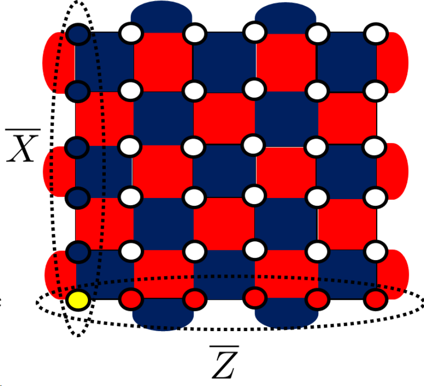
At the parameter values $h_{z,i,1}=h_{x,1,j}=\pi/2$ and $h_{z,i,j\neq 1}=h_{x,i\neq 1,j}=0$ (to be referred to as ideal values onwards), the first and second exponentials of Eq. (1) reduce to perfect logical $Z$ and $X$ gates respectively, i.e., $\overline{Z}=\prod_{i=1}^{L_{x}}Z_{i,1}$ and $\overline{X}=\prod_{j=1}^{L_{y}}X_{1,j}$ in Fig. 1. In this case, by denoting $|\overline{0}\rangle$ and $|\overline{1}\rangle$ as the logical basis states in the simultaneous $+1$ eigenspace of all the stabilizer operators $\mathcal{S}_{X,i,j}$, $\mathcal{S}_{Z,i,j}$, $\mathcal{S}_{X,i,j}^{\rm boundary}$, and $\mathcal{S}_{Z,i,j}^{\rm boundary}$, one may explicitly construct two of the system’s Floquet eigenstates as

with quasienergies

and $\varepsilon_{0,-}=\varepsilon_{0,+}+\pi/T$. In particular, the state $|\overline{0}\rangle$ transforms into $|\overline{1}\rangle$ over one period and vice versa, leading to a $2T$-periodicity capturable by the operator $\overline{Z}$. While $|\overline{0}\rangle$ and $|\overline{1}\rangle$ are highly entangled states, it can further be shown that $2T$-periodicity persists with respect to product states that can be written as superposition of logical states belonging to different stabilizer subspaces. An example of such a state is $|0\cdots 0\rangle$, which can also be written as

where $\left\{\mathcal{S}_{Z,k},\mathcal{S}_{X,k}\right\}$ is the set of all $Z$ and $X$ stabilizers (including boundary operators).

Away from the ideal values above, the system is no longer integrable. Nevertheless, one may write the Floquet operator as

where $U_{T,\rm ideal}$ is the Floquet operator associated with the ideal values,

$\delta_{z,i,j}$ and $\delta_{x,i,j}$ are deviations in $h_{z,i,j}$ and $h_{x,i,j}$ from their respective ideal values. The evolution of a logical state, e.g., $|\overline{0}\rangle$, after one period can then be written as

where $|\varepsilon\rangle$ is a Floquet eigenstate of $U_{T,\rm ideal}$. By expanding the exponentials of $\tilde{U}_{T}$ as superpositions of products of $X_{1,j}$ and $Z_{i,1}$, it follows that nonzero contributions to $\langle\varepsilon_{0,\pm}|\tilde{U}_{T}|\overline{1}\rangle$ come from identity, which leads to a relative $\pi$ phase between $|\varepsilon_{0,\pm}\rangle$, as well as $\prod_{j}^{L_{y}}X_{1,j}$ or $\prod_{i}^{L_{x}}Z_{i,1}$, which only appear at order $\sin^{L_{y}}(\delta_{x})$ or $\sin^{L_{x}}(\delta_{z})$ respectively. Indeed, lower weight Pauli operators bring $|\overline{1}\rangle$ outside the logical subspace, resulting in a state of zero overlap with $|\varepsilon_{0,\pm}\rangle$. Consequently, an imperfection of order $\sin(\delta_{x}),\sin(\delta_{Z})\sim\epsilon$ will only result in the relative phase deviation from $\pi$ by an order of $\epsilon^{\mathrm{min}(L_{x},L_{y})}$.

Despite the similarity of the above feature with known DTC models based on quantum repetition code DTC2, two main differences exist. First, a nonlocal order parameter, e.g., $\overline{Z}$, is necessary for capturing the $2T$ periodicity in the present system. Second, note that the usual DTC models typically only supports a single subharmonic order parameter dynamics, e.g., magnetization pointing in a specific direction. By contrast, at least two nonlocal observables with subharmonic dynamics exist in the present system, i.e., $\overline{Z}$ and $\overline{X}$. To support this point, Fig. 2 displays the stroboscopic dynamics of $\overline{Z}$ and $\overline{X}$ for a surface code of two different sizes. There, robust $2T$ periodic profile is clearly evident in all cases despite the presence of considerable imperfection in the parameters $h_{x,j}$ and $h_{z,j}$ responsible for enacting the logical $X$ and $Z$ gate.

Figure 3 further reveals that increasing $L_{y}$ while fixing $L_{x}$ clearly improves the $2T$ oscillation profile of $\langle\overline{Z}\rangle$, but leaves that of $\langle\overline{X}\rangle$ to be qualitatively the same. This can be intuitively understood by inspecting the relative phase $\xi_{\overline{Z}}=\mathrm{i}\;\mathrm{log}\frac{\langle\varepsilon_{0,-}|\tilde{U}_{T}|\overline{1}\rangle}{\langle\varepsilon_{0,+}|\tilde{U}_{T}|\overline{1}\rangle}$ and $\xi_{\overline{X}}=\mathrm{i}\;\mathrm{log}\frac{\langle\varepsilon_{0,-}|\tilde{U}_{T}|\overline{+}\rangle}{\langle\varepsilon_{0,+}|\tilde{U}_{T}|\overline{+}\rangle}$ (recall Eqs. (6)-(8)), where $|\overline{+}\rangle=(|\overline{0}\rangle+|\overline{1}\rangle)/\sqrt{2}$. In particular, the initial state $|\overline{1}\rangle$ ($|\overline{+}\rangle$) leads to period-doubling in $\langle\overline{Z}\rangle$ ($\langle\overline{X}\rangle$) if $\xi_{\overline{Z}}\approx\pi$ ($\xi_{\overline{X}}\approx\pi$). By expanding $\tilde{U}_{T}$ as a superposition of products of $X_{i,j}$ and $Z_{i,j}$, it follows that the lowest order correction to $\xi_{\overline{X}}$ ($\xi_{\overline{Z}}$) from its ideal value of $\pi$ occurs at the $L_{x}$-($L_{y}$-)th order, which corresponds to terms $\propto\overline{Z}$ ($\propto\overline{X}$). This argument can be straightforwardly extended to any other eigenstate $|\psi_{0}\rangle$ of $H_{S,\rm surface}$. In this case, one may find two quasienergy eigenstates $|\varepsilon_{n,\pm}\rangle$ of $U_{T,\rm ideal}$ with $\pi/T$ spacing that satisfy $|\psi_{0}\rangle\propto|\varepsilon_{n,+}\rangle+|\varepsilon_{n,-}\rangle$. It then follows that $\mathrm{i}\;\mathrm{log}\frac{\langle\varepsilon_{n,-}|\tilde{U}_{T}|\psi_{0}\rangle}{\langle\varepsilon_{n,+}|\tilde{U}_{T}|\psi_{0}\rangle}\approx\pi$ up to a correction of order at least $\epsilon^{L_{x}}$ or $\epsilon^{L_{y}}$. Finally, by noting that any generic initial state can be expanded in terms of $U_{T,\rm ideal}$ eigenstates, one concludes that the deviation from a perfect period-doubling in $\langle\overline{X}\rangle$ ($\langle\overline{Z}\rangle$) is suppressed through an increase in $L_{x}$ ($L_{y}$), which agrees with the observation in Fig. 3.

We have introduced a periodically driven surface code and highlighted its nonlocal DTC phase. Unlike other previously studied DTCs, a nonlocal order parameter is neccesary for capturing its subharmonic signature. The nonlocal generalization of the spectral functions, spin-glass order parameters, and two-point correlators are further introduced to distinguish such nonlocal DTCs from trivial paramagnets. These metrics further allow the characterization of the system’s other phases, which include the trivial paramagnetic and “surface code” phase. The latter is topologically equivalent to the static surface code system in the absence of magnetic field.

The nonlocal DTCs observed in this paper are also expected to exist in a variety of other topologically ordered systems. To this end, a comprehensive study of other periodically driven topological quantum error correction codes, e.g., the color codes color1; color2, the Majorana version of the surface codes Majsur, or the quantum double models toric, thus represents a promising direction for future work. In this case, the three nonlocal metrics introduced above will further open an opportunity for discovering other exotic phases in these systems. To improve their experimental feasibility beyond trapped ions and Sycamore platforms, it will also be interesting to explore the possibility of observing nonlocal DTCs with continuous driving. Finally, given that nonlocal DTCs share similar physics as that of topological quantum error correction codes, their potential application in quantum computing poses another interesting open question worth exploring.

Note added: During the finalization of this work, we came across a recent similar preprint similar proposing a new type of discrete time crystal in periodically driven topological ordered systems, with a particular example on the periodically driven surface codes. Despite the similarity in the model under study, Ref. similar focuses on rigorously establishing the theory of topologically-ordered time crystals (equivalent to nonlocal DTCs introduced here), whereas this work focuses on characterizing the various phases of the system under both periodic and open boundary conditions.

References

- (1) F. Wilczek, Phys. Rev. Lett. 109, 160401 (2012).
- (2) A. Shapere and F. Wilczek, Phys. Rev. Lett. 109, 160402 (2012).
- (3) P. Bruno, Phys. Rev. Lett. 111, 070402 (2013).
- (4) H. Watanabe and M. Oshikawa, Phys. Rev. Lett. 114, 251603 (2015).
- (5) V. K. Kozin and O. Kyriienko, Phys. Rev. Lett. 123, 210602 (2019).
- (6) J. Zhang, P. W. Hess, A. Kyprianidis, P. Becker, A. Lee, J. Smith, G. Pagano, I.-D. Potirniche, A. C. Potter, A. Vishwanath, N. Y. Yao, and C. Monroe, Nature (London) 543, 217 (2017).
- (7) S. Choi, J. Choi, R. Landig, G. Kucsko, H. Zhou, J. Isoya, F. Jelezko, S. Onoda, H. Sumiya, V. Khemani, C. v. Keyserlingk, N. Y. Yao, E. Demler, and M. D. Lukin, Nature (London) 543, 221 (2017).
- (8) J. Rovny, R. L. Blum, and S. E. Barrett, Phys. Rev. Lett. 120, 180603 (2018).
- (9) J. Rovny, R. L. Blum, and S. E. Barrett, Phys. Rev. B 97, 184301 (2018).
- (10) S. Pal, N. Nishad, T. S. Mahesh, and G. J. Sreejith, Phys. Rev. Lett. 120, 180602 (2018).
- (11) S. Autti, P. J. Heikkinen, J. T. Mäkinen, G. E. Volovik, V. V. Zavjalov and V. B. Eltsov, Nat. Mater. (2020).
- (12) A. Kyprianidis, F. Machado, W. Morong, P. Becker, K. S. Collins, D. V. Else, L. Feng, P. W. Hess, C. Nayak, G. Pagano, N. Y. Yao, and C. Monroe, Science 372, 1192-1196 (2021).
- (13) K. Sacha, Phys. Rev. A 91, 033617 (2015).
- (14) D. V. Else, B. Bauer, and C. Nayak, Phys. Rev. Lett. 117, 090402 (2016).
- (15) D. V. Else, B. Bauer, and C. Nayak, Phys. Rev. X 7, 011026 (2017).
- (16) C. W. von Keyserlingk and S. L. Sondhi, Phys. Rev. B 93, 245146 (2016).
- (17) V. Khemani, A. Lazarides, R. Moessner, and S. L. Sondhi, Phys. Rev. Lett. 116, 250401 (2016).
- (18) N. Y. Yao, A. C. Potter, I.-D. Potirniche, and A. Vishwanath, Phys. Rev. Lett. 118, 030401 (2017).
- (19) W. W. Ho, S. Choi, M. D. Lukin, and D. A. Abanin, Phys. Rev. Lett. 119, 010602 (2017).
- (20) B. Huang, Y.-H. Wu, and W. V. Liu, Phys. Rev. Lett. 120, 110603 (2018).
- (21) A. Russomanno, F. lemini, M. Dalmonte, and R. Fazio, Phys. Rev. B 95, 214307 (2017).
- (22) A. Russomanno, B. E. Friedman, and E. G. D. Torre, Phys. Rev. B 96, 045422 (2017).
- (23) W. C. Yu, J. Tangpanitanon, A. W. Glaetzle, D. Jaksch, and D. G. Angelakis, Phys. Rev. A 99, 033618 (2019).
- (24) C. Fan, D. Rossini, H.-X. Zhang, J.-H. Wu, M. Artoni, G. C. L. Rocca, Phys. Rev. A 101, 013417 (2020).
- (25) F. Machado, D. V. Else, G. D. K.-Meyer, C. Nayak, N. Y. Yao, Phys. Rev. X 10, 011043 (2020).
- (26) P. Nurwantoro, R. W. Bomantara, and J. Gong, Phys. Rev. B 100, 214311 (2019).
- (27) K. Giergiel, A. Kosior, P. Hannaford, K. Sacha, Phys. Rev. A 98, 013613 (2018).
- (28) K. Giergiel, A. Kuros, K. Sacha, Phys. Rev. B 99, 220303 (2019).
- (29) K. Giergiel, T. Tran, A. Zaheer, A. Singh, A. Sidorov, K. Sacha, P. Hannaford, New J. Phys. 22, 085004 (2020).
- (30) A. Kosior, K. Sacha, Phys. Rev. A 97, 053621 (2018).
- (31) P. Matus, K. Sacha, Phys. Rev. A 99, 033626 (2019).
- (32) A. Russomanno, S. Notarnicola, F. M. Surace, R. Fazio, M. Dalmonte, M. Heyl, Phys. Rev. Res. 2, 012003 (2020).
- (33) F. M. Surace, A. Russomanno, M. Dalmonte, A. Silva, R. Fazio, F. Iemini, Phys. Rev. B 99, 104303 (2019).
- (34) F. Iemini, A. Russomanno, J. Keeling, M. Schiro, M. Dalmonte, R. Fazio, Phys. Rev. Lett. 121, 035301 (2018).
- (35) G. Zlabys, C.-h. Fan, E. Anisimovas, K. Sacha, Phys. Rev. B 103, 100301 (2021).
- (36) A. Kuros, R. Mukherjee, W. Golletz, F. Sauvage, K. Giergiel, F. Mintert, K. Sacha, New. J. Phys. 22, 095001 (2020).
- (37) J. Wang, P. Hannaford, and B. J. Dalton, New. J. Phys. 23, 063012 (2021).
- (38) O. Shtanko and R. Movassagh, Phys. Rev. Lett. 125, 086804 (2020).
- (39) D. T. Liu, J. Shabani, A. Mitra, Phys. Rev. B 99, 094303 (2019).
- (40) K. Sacha, Time Crystals (Springer, Switzerland, 2020).
- (41) D. V. Else, C. Monroe, C. Nayak, and N. Y. Yao, Annu. Rev. Condens. Matter Phys. 11, 467-499 (2020).
- (42) V. Khemani, R. Moessner, S. L. Sondhi, arXiv:1910.10745v1.
- (43) K. Sacha, J. Zakrzewski, Rep. Prog. Phys. 81, 016401 (2017).
- (44) R. W. Bomantara and J. B. Gong, Phys. Rev. Lett. 120, 230405 (2018).
- (45) A. Kshetrimayum, M. Goihl, D. M. Kennes, J. Eisert, Phys. Rev. B 103, 224205 (2021).
- (46) M. Ippoliti, K. Kechedzhi, R. Moessner, S. L. Sondhi, and V. Khemani, arXiv:2007.11602v1.
- (47) K. Sacha, Sci. Rep. 5, 10787 (2015).
- (48) D. Delande, L. Morales-Molina, and K. Sacha, Phys. Rev. Lett. 119, 230404 (2017).
- (49) K. Giergiel and K. Sacha, Phys. Rev. A 95, 063402 (2017).
- (50) M. Mierzejewski, K. Giergiel, and K. Sacha, Phys. Rev. B 96, 140201(R) (2017).
- (51) K. Giergiel, A. Miroszewski, and K. Sacha, Phys. Rev. Lett. 120, 140401 (2018).
- (52) R. W. Bomantara, arXiv:2102.09113.
- (53) E. Knill, R. Laflamme, and W. Zurek, arXiv:quantph/9610011 [quant-ph].
- (54) A. Y. Kitaev, Russian Math. Surveys 52, 1191 (1997)
- (55) E. Dennis, A. Kitaev, A. Landahl, and J. Preskill, J. Math. Phys. 43, 4452 (2002).
- (56) J. Roffe, Contem. Phys. 60, 226-245 (2019).
- (57) P. W. Shor, Phys. Rev. A 52, R2493 (1995).
- (58) J. R. Wootton and D. Loss, Phys. Rev. A 97, 052313 (2018).
- (59) J. Kelly et al, Nature 519, 66-69 (2015).
- (60) A. G. Fowler, M. Mariantoni, J. M. Martinis, and A. N. Cleland, Phys. Rev. A 86, 032324 (2012).
- (61) A. Kitaev, Ann. Phys. 303, 2 (2003).
- (62) S. B. Bravyi and A. Y. Kitaev, arXiv:quant-ph/9811052 [quant-ph] (1998).
- (63) B. J. Brown, Sci. Adv. 6, eaay4929, (2020).
- (64) J. P. B.-Ataides, D. K. Tuckett, S. D. Bartlett, S. T. Flammia, B. J. Brown, Nat. Commun. 12, 2172 (2021).
- (65) J. H. Shirley, Phys. Rev. 138, B979 (1965).
- (66) H. Sambe, Phys. Rev. A 7, 2203 (1973).
- (67) D. A. Abanin, W. De Roeck, and F. Huveneers, Ann. Phys. (Amsterdam) 372, 1 (2016).
- (68) P. Ponte, A. Chandran, Z. Papic, and D. A. Abanin, Ann. Phys. (Amsterdam) 353, 196 (2015).
- (69) P. Ponte, Z. Papic, F. Huveneers, and D. A. Abanin, Phys. Rev. Lett. 114, 140401 (2015).
- (70) A. Lazarides, A. Das, and R. Moessner, Phys. Rev. Lett. 115, 030402 (2015).
- (71) D. V. Else, W. W. Ho, and P. T. Dumitrescu, Phys. Rev. X 10, 021032 (2020).
- (72) G. J. Sreejith, A. Lazarides, and R. Moessner, Phys. Rev. B 94, 045127 (2016).
- (73) R. W. Bomantara, S. Mu, and J. Gong, Phys. Rev. B 103, 235404 (2021).
- (74) A. Y. Kitaev, Ann. Phys. 321, 2 (2006).
- (75) F. Arute et al, Nature 574, 505 (2019).
- (76) H. Bombin and M. A. M.-Delgado, Phys. Rev. Lett. 97, 180501 (2006).
- (77) B. J. Brown, N. H. Nickerson, D. E. Browne, Nat. commun. 7, 12302 (2016).
- (78) S. Vijay, T. H. Hsieh, and L. Fu, Phys. Rev. X 5, 041038 (2015).
- (79) T. B. Wahl, B. Han, and B. Béri, arXiv:2105.09694.