Testing Directed Acyclic Graph via Structural,
Supervised and Generative Adversarial Learning
Abstract
In this article, we propose a new hypothesis testing method for directed acyclic graph (DAG). While there is a rich class of DAG estimation methods, there is a relative paucity of DAG inference solutions. Moreover, the existing methods often impose some specific model structures such as linear models or additive models, and assume independent data observations. Our proposed test instead allows the associations among the random variables to be nonlinear and the data to be time-dependent. We build the test based on some highly flexible neural networks learners. We establish the asymptotic guarantees of the test, while allowing either the number of subjects or the number of time points for each subject to diverge to infinity. We demonstrate the efficacy of the test through simulations and a brain connectivity network analysis.
Key Words: Brain connectivity networks; Directed acyclic graph; Hypothesis testing; Generative adversarial networks; Multilayer perceptron neural networks.
1 Introduction
Directed acyclic graph (DAG) is an important tool to characterize pairwise associations among multivariate and high-dimensional random variables. It has been frequently used in a wide range of scientific applications. One example is gene regulatory network analysis in genetics (Sachs et al. 2005), where the time-course expression data of multiple genes are measured over multiple cellular samples through microarray or RNA sequencing, and the goal is to understand the regulatory activation or repression relations among different genes. Another example is brain effective connectivity analysis in neuroscience (Garg et al. 2011), where the time-course neural activities are measured at multiple brain regions for multiple experimental subjects through functional magnetic resonance imaging, and the goal is to infer the influences of brain regions exerting over each other under the stimulus.
There is a large body of literature studying penalized estimation of DAG given the observational data (see, e.g., Spirtes et al. 2000; van de Geer and Bühlmann 2013; Zheng et al. 2018; Yuan et al. 2019, among many others). These works all impose some specific model structures, most often, linear models or additive models. There have recently emerged a number of proposals in the computer science literature that used neural networks or reinforcement learning to tackle nonlinear models and to estimate the associated DAG (Yu et al. 2019; Zheng et al. 2020; Zhu et al. 2020). While all these works have made crucial contributions, DAG model estimation is an utterly different problem from DAG inference. By inference, we mean hypothesis testing of individual edges throughout this article. The two problems are closely related, and both can, in effect, identify important links of a DAG. Besides, DAG inference usually relies on DAG estimation as a precedent step. Nevertheless, estimation does not produce an explicit quantification of statistical significance as inference does. Bayesian networks have been proposed for DAG estimation and inference. However, computationally, it is extremely difficult to search through all possible graph structures in a Bayesian network (Chickering et al. 2004), and as a result, the dimension of the Bayesian network is often small (Friston 2011). There are very few frequentist inference solutions for inferring DAG structures. Only recently, Janková and van de Geer 2019 proposed a de-biased estimator to construct confidence intervals for the edge weights in a DAG, whereas Li et al. 2020 developed a constrained likelihood ratio test to infer individual edges or some given directed paths of a DAG. These works are probably the most relevant to our proposal. However, both have focused on Gaussian linear DAG, and cannot be easily extended to more general nonlinear DAG models. Moreover, all the above works considered the setting where the data observations are independent and identically distributed (i.i.d.). Learning DAG from time-dependent data remains largely unexplored.
There is another body of literature studying conditional independence testing (CIT); see Li and Fan 2019; Shah and Peters 2020; Shi et al. 2021 and the references therein. CIT is closely related to DAG inference, and is to serve as a building block of our proposed testing procedure. On the other hand, naively performing CIT on two variables given the rest would fail to infer the directed edges of a DAG; see Section 2.2 for details. Besides, most CIT methods assume the data observations are independent, and are not suitable for the setting where the measurements are time-dependent.
In this article, we propose a novel statistical testing procedure for the inference of individual links or some given paths in a large and general DAG. The new test hinges upon some highly flexible neural networks-based machine learning techniques. The associations among the random variables can be either linear or nonlinear, the variables themselves can be either continuous or discrete-valued, and the observed data can be time-dependent.
Methodologically, we employ a number of state-of-the-art deep learning techniques that are highly flexible and can capture nonlinear associations among high-dimensional variables. We begin with a new characterization of directed edges under the additive noise structure (Peters et al. 2014); see Theorem 1. Based on this characterization, we propose a new testing procedure that integrates three key deep learning ingredients: (a) a DAG structural learning method based on neural networks or reinforcement learning to estimate the DAG; (b) a supervised learning method based on neural networks to estimate the conditional mean; and (c) a distribution generator produced by generative adversarial networks (Goodfellow et al. 2014, GANs) to approximate the conditional distribution of the variables in the DAG. We further couple these deep learning tools with some hypothesis testing strategies, including data splitting and cross-fitting to ensure a valid size control, and constructing a doubly robust test statistic as the maximum of multiple transformation functions to improve the power.
Theoretically, we establish the asymptotic size and power guarantees for the proposed test. The data-splitting and cross-fitting strategy ensures that our test achieves a valid type-I error control asymptotically under minimal conditions on those learning methods. As a result, our test procedure can work with a wide range of nonparametric estimators. Next, our DAG testing procedure requires a DAG estimation solution as a precedent step, which is common for almost all graph inference approaches (Cai 2017). However, we do not assume the ordering of the nodes is known a priori, but instead estimate this DAG ordering from the data using some DAG structural learning method. To establish the consistency of the proposed test, we require this ordering is consistently estimated; see condition (C1). Nevertheless, this order consistency is much weaker than requiring the initial DAG estimator to be selection consistent, or to satisfy the sure screening property. In other words, we only require a reasonably good initial estimator of DAG, which is order consistent but not necessarily selection consistent. We then develop a testing procedure that produces an explicit quantification of statistical significance for each individual link, and we show the test has the desired size and power guarantees. We also prove that the estimator from the DAG structural learning method we employ is indeed order consistent. Meanwhile, we discuss the impact on our test when this order consistency condition is not satisfied. Finally, for our theoretical analysis, we introduce a bidirectional asymptotic framework that allows either the number of subjects, or the number of time points for each subject, to diverge to infinity. This is useful for different types of applications. There are plenty of studies where the interest is about the general population, and thus it is reasonable to let the number of subjects or samples to diverge. Meanwhile, there are plenty of other applications, e.g., neuroimaging-based brain networks studies, where the number of subjects is almost always limited, but the scanning time and the temporal resolution can greatly increase. For those applications, it is more suitable to let the number of time points to diverge.
Our proposal is innovative and makes useful contributions in several ways.
First, rigorous inference of directed edges in DAG is a vital but also a long-standing open question. The existing solutions rely on particular model structures such as linear or additive models, and mostly deal with i.i.d. data. Such requirements can be restrictive in numerous applications, since the actual relations may be nonlinear and the data are correlated. By contrast, we only require an additive noise structure. To the best of our knowledge, our work is the first frequentist hypothesis testing solution for a general DAG with time-dependent data.
Second, we employ modern deep learning techniques such as neural networks and GANs to help address a classical statistical hypothesis testing problem. Such modern learning methods serve as nonparametric learners, and conceptually, play a similar role as splines and reproducing kernels. Meanwhile, they are often more flexible and can handle more complex data structures. With increasingly efficient implementations of these methods and improved understandings of their theoretical properties (Bauer and Kohler 2019; Farrell et al. 2021, e.g.,), this family of deep learning methods offer a powerful set of tools for classical statistical problems. Our proposal can be viewed as one of the early examples of harnessing such power, as the use of these deep learning techniques allows us to accurately estimate the DAG structure, the conditional means, as well as the distribution functions, and to improve the power of the test.
Third, even though the individual learning components such as neural networks, GANs and cross-fitting are not completely new, how to integrate them properly and effectively into a test with desired theoretical guarantees is highly nontrivial, and is one of the main contributions of this article. In effect, our proposed test achieves a parametric convergence rate and a parametric power guarantee while using nonparametric estimators. This is made possible mainly due to the innovative way we put together these learning components, which leads to a doubly robust test statistic (Tsiatis 2007), in the sense that the proposed statistic is consistent, as long as either the conditional mean function in (b), or the distribution generator in (c) is correctly specified. In our solution, we propose to estimate both the conditional mean and the distribution generator fully nonparametrically. As such, the convergence rate of the two estimators, denoted by and , respectively, may each be slower than the parametric rate. Nevertheless, we only require , which is totally achievable for the multilayer perceptron models and GANs; see the discussion after condition (C4). The key idea of our theoretically analysis is to show the bias of the estimating equation grows faster than the parametric rate. Thanks to the double robustness property of the test statistic, if we replace either estimator with its oracle value, the bias would be equal to zero. This observation, together with the Neyman orthogonality property of the estimating equation, ensures that the bias can be represented as a product of the difference between the two nonparametric estimators and their oracle values. Consequently, when , the test statistic converges at a parametric rate, the corresponding test controls the type-I error, and has a parametric power guarantee. We comment that, in their seminal work on double/debiased machine learning, Chernozhukov et al. 2018 proposed to combine two machine learning estimators to infer the average treatment effect, which they showed to achieve a parametric convergence rate, even though each of the machine learning estimator converges at a nonparametric rate. Our result is similar in spirit as theirs, but targets a completely different problem, and thus is the first of its kind for DAG inference.
The rest of the article is organized as follows. We formally define the hypotheses, along with the model and data structure, in Section 2. We develop the testing procedure in Section 3, and establish the theoretical properties in Section 4. We study the empirical performance of the test through simulations and a real data example in Sections 5 and 6. We relegate several extensions, additional results, and all technical proofs to the Supplementary Appendix.
2 Problem Formulation
In this section, we first present the DAG model, based on which we formally define our hypotheses. We next propose an equivalent characterization of the hypotheses, for which we develop our testing procedure. Finally, we detail the data structure.
2.1 DAG model
Consider random variables , each with a finite fourth moment. We use a directed graph to characterize the relationships among these variables, where a node of the graph corresponds to a variable in . For two nodes , if an arrow is drawn from to , i.e., , then is called a parent of , and a child of . A directed path in the graph is a sequence of distinct nodes , such that there is a directed edge for all . If there exists a directed path from to , then is called an ancestor of , and a descendant of . For node , let and denote the set of indices of the parents, descendants, and ancestors of , respectively. Moreover, let denote the sub-vector of formed by those whose indices are in a subset .
To rigorously formulate our problem, we make two assumptions.
- (A1)
The directed graph is acyclic; i.e., no variable is an ancestor of itself.
- (A2)
The DAG is identifiable from the joint distribution of .
Condition (A1) has been commonly imposed in directed graph analysis. It does not permit any variable to be its own ancestor. As a result, the relationship between any two variables is unidirectional. Condition (A2) helps simplify the problem, and avoids dealing with the equivalence class of DAG. This condition is again frequently imposed in the DAG estimation literature (Zheng et al. 2018; Yuan et al. 2019; Li et al. 2020; Zheng et al. 2020). We discuss the extension to the equivalence class in Section A.4 of the Appendix.
We consider a class of structural equation models that follow an additive noise structure,
| (1) |
where are a set of continuous functions, and are a set of independent zero mean random errors. Model (1) permits a fairly flexible structure. For instance, if each is a linear function, then (1) reduces to a linear structural equation model. If each is an additive function, i.e., , then (1) becomes an additive model. In our test, we do not impose linear or additive model structures. Moreover, we can easily extend the proposed test to the setting of generalized linear model, where the can be either continuous or discrete-valued. We discuss such an extension in Section A.3 of the Appendix.
Under model (1), the corresponding DAG is identifiable under some reasonable conditions. We consider three examples to discuss explicitly those conditions.
Example 1 (Gaussian graphical model).
Suppose are jointly normal, and model (1) becomes , for some and . Then the corresponding DAG is identifiable, if the variance of the random error is the same for all (Bühlmann et al. 2014, Theorem 1).
Example 2 (Nonlinear graphical model with Gaussian noise).
Suppose are jointly normal, but are not. Then the corresponding DAG is identifiable, if each is three times differentiable and not linear in any of its arguments (Peters et al. 2014, Corollary 31).
Example 3 (Nonlinear graphical model with general noise).
Suppose neither nor is normal. Then the corresponding DAG is identifiable, if each is non-constant in each of its arguments, and (1) is a restricted additive noise model (Peters et al. 2014, Definition 27).
2.2 Hypotheses and equivalent characterization
We next formally define the hypotheses we target, then give an equivalent characterization. For a given pair of nodes , , we aim at the hypotheses:
| (2) |
When the alternative hypothesis holds, there is a link from to . In the following, we mainly focus on testing an individual link . We discuss the extension of testing a directed pathway, or a union of links, in Section A.1 and Section A.2 of the Appendix.
We next consider a pair of hypotheses that involve two variables that are conditionally independent (CI). The new hypotheses are closely related to (2), but are not exactly the same.
| (3) |
We point out that, testing for (3) is generally not the same as testing for (2). To elaborate this, we consider a three-variable DAG with a v-structure.
Example 4 (v-structure).
Consider three random variables that form a v-structure, as illustrated in Figure 1(a), where and are the common parents of . Even if and are marginally independent, they can be conditionally dependent given . To better understand this, consider the following toy illustration. Either the ballgame or the rain could cause traffic jam, but they are uncorrelated. However, seeing traffic jam puts the ballgame and the rain in competition as a potential explanation. As such, these two events are conditionally dependent. Since is not a parent of , both and hold. Consequently, testing for (3) can have an inflated type-I error for testing (2).
 |
 |
 | ||
| (a) | (b) | (c) |
In this example, we see the reason that testing for (3) is not the same as for (2) is because the conditioning set of and contains their common descendant . This key observation motivates us to consider a variant of (3), which we show is equivalent to (2) under certain conditions. We also remark that missing links in a DAG correspond to specific conditional independence between variables, but are not equivalent to marginal independence in general.
Specifically, for a given set of indices such that , and letting denote the set of variables in , we consider the hypotheses:
| (4) |
Proposition 1.
Proposition 1 forms the basis for our test. That is, to infer the directed links, we first restrict our attention to the pairs such that . Apparently, does not hold when . Next, when devising a conditional independence test for , the conditioning set is supposed to contain the parents of node , but cannot contain any common descendants of . Under these conditions, we establish the equivalence between (4) and (2). A similar idea of using CI tests for DAG structural learning was employed in Spirtes et al. 2000 too.
Next, we develop a test statistic for the hypotheses (4). We introduce a key quantity. Let denote a square-integrable function that takes and as the input. Define
Under the additive noise model (1), the next theorem connects this quantity with the null hypothesis in (4). Together with Proposition 1, it shows that can serve as a test statistic for (4), and equivalently, for (2) that we target.
Theorem 1.
Theorem 1 immediately suggests a possible testing procedure for (4). That is, we first employ a DAG estimator to learn the ancestors and descendants for node . We then consider a natural choice for , where . Then becomes
| (5) |
By Theorem 1, under the null hypothesis , a consistent estimator for (5) should be close to zero. A Wald type test can then be devised with i.i.d. data. That is, we first obtain an estimator for , by plugging in the estimators of the conditional mean functions, and . We then get an estimator of its asymptotic variance , and obtain the Wald type test statistic, , where is the number of samples. Such a test is similar in spirit as the tests of Zhang et al. 2018 and Shah and Peters 2020. Since it involves estimation of two conditional mean functions, we refer to it as the double regression-based test. We later numerically compare our proposed test with this test.
On the other hand, this double regression-based test has some limitations. One is that it requires the set to be fixed. To meet the requirement in Proposition 1, needs to be determined in a data-adaptive way. The resulting test may not control the type-I error due to the dependence between and the estimator of the mean functions in . Another limitation is that it may not have a sufficient power to detect . As an illustration, we revisit Example 4. For this example, consider the structural equation model: , , and . Under this model, holds. Meanwhile, . When the distribution of is symmetric, , despite the fact that is a parent of . As such, for this example, the double regression-based test is to have no power at all.
To address the first limitation, we employ the sample splitting strategy to ensure its size control. To address the second limitation, we consider multiple transformation functions , instead of a single , to improve the power. We detail our idea in Section 3.
2.3 Time-dependent observational data
Throughout this article, we use to denote the population variables, and to denote the data realizations. Suppose the data come from an observational study, and are of the form, , where indexes the th subject, indexes the th time point, and indexes the th random variable. Suppose there are totally subjects, with observations for the th subject. Write , . We consider the following data structure.
- (B1)
Across subjects, the measurements , , are i.i.d.
- (B2)
Across time points, the random vectors , , are stationary.
- (B3)
For any , , , are DAG-structured. In addition, their joint distribution is the same as that of .
Condition (B1) is reasonable, as the subjects are usually independent from each other. We do not study the scenario where the data come from the same families or clusters. Condition (B2) about the stationarity is common in numerous applications such as brain connectivity analysis (Bullmore and Sporns 2009; Qiu et al. 2016; Wang et al. 2016). Condition (B3) brings the data into the DAG framework that we study. Note that (B3) does not allow directed edges from past to future observations. Meanwhile, we discuss the extensions of our test for non-stationary DAG, or for past to future edges, in Section A.5 of the Appendix.
3 Testing Procedure
In this section, we develop an inferential procedure for the hypotheses in (2) for a given pair , through (4), given the observational data . We first present the main ideas and the complete procedure, then detail the major steps. As our test is based on Structural learning, sUpervised learning, and Generative AdveRsarial networks, we call our method SUGAR.
3.1 The main algorithm
Our main idea is to construct a series of measures , for a large number of transformation functions , then take the maximum of some standardized version of . Toward that goal, our test involves three key components:
- (a)
A DAG structural learning method to learn the set of indices that satisfy Proposition 1;
- (b)
A supervised learning method to estimate the conditional mean function ;
- (c)
A distribution generator to approximate the conditional distribution of the variables.
For (a), we apply a structural learning algorithm to learn the underlying DAG corresponding to . The input of this step is the observed data , and the output is the estimated DAG. We then set as the estimated set of ancestors of . To capture possible sparsity and nonlinear associations in , we employ the DAG estimation method of Zheng et al. 2020. See Section 3.3 for details.
For (b), we employ a supervised learning algorithm. The input of this step is that serves as the “predictors”, and that serves as the “response”, and the output is the estimated mean function . We employ a multilayer perceptron learner, which has a good capacity of estimating complex high-dimensional mean, and the estimator has the desired consistency guarantees (Farrell et al. 2021). See Section 3.4 for details.
For (c), we propose to use generative adversarial networks (Goodfellow et al. 2014, GANs) to approximate the conditional distribution of given . The input of this step is and multivariate Gaussian noise vectors, and the output is the learnt generator model, with a set of pseudo samples , , that have a similar distribution as the training samples. We employ a generator model with the Sinkhorn divergence loss (Genevay et al. 2018) to mitigate the potential bias of GANs. See Section 3.5 for details.
Given the generated pseudo samples, we then proceed to estimate the conditional mean function in (5), and construct the corresponding test statistic. We also incorporate the data-splitting and cross-fitting strategy (Romano and DiCiccio 2019), to ensure a valid type-I error control for the test under minimal conditions for the above three learners. Specifically, we randomly split the samples into two equal halves , where denotes the set of subsample indices, . We then compute the three learners in (a) to (c) using each half of the data separately. Based on these learners, we next use cross-fitting to estimate , and their associated standard deviations. We construct our test statistic as the largest standardized version of in the absolute value. This leads to two Wald-type test statistics, one for each half of the data. Finally, we derive the -values based on Gaussian approximation, and reject the null when either one of the -value is smaller than . By Bonferroni’s inequality, this yields a valid -level test. See Section 3.2 for details.
A summary of the proposed testing procedure is given in Algorithm 1.
- Step 1.
Randomly split the data into two equal halves, , .
- Step 2.
For each half of the data, ,
- (2a)
Apply the structural learning method (9) to estimate the DAG . Denote the estimated set of ancestors of by . Set .
- (2b)
If , return the -value, .
- (2a)
- Step 3.
For , apply the supervised learning method (10) to estimate the conditional mean function , and denote the estimator by .
- Step 4.
For , apply the GANs method to learn a generator model to approximate the conditional distribution of given . It returns the learnt generator , and a set of pseudo samples .
- Step 5.
Construct the test statistic:
- (5a)
Randomly generate functions from the class in (6).
- (5b)
For each , construct two standardized measures, and , with and without cross-fitting, using (7).
- (5c)
Select the index, , based on the measure without cross-fitting.
- (5d)
Set the test statistic as , based on the measure with cross-fitting.
- (5a)
- Step 6.
Return the -value:
- (6a)
Compute the -value, , for each half of the data, , where is a standard normal random variable.
- (6b)
Return .
- (6a)
3.2 Test statistic and -value
We begin with the presentation of our test, including the test statistic and the computation of the -value, which are built on the three learners in (a) to (c) that we discuss in detail later.
First, for each half of the data, , we begin with a bounded function class , indexed by some parameter . In our implementation, we consider the class of characteristic functions of ,
| (6) |
We note that (6) is not able to approximate the entire class of square integrable functions. Nevertheless, our numerical experiments have found that setting according to (6) results in a good power empirically. Moreover, we note that one may set to the class of characteristic functions of . By the Fourier Theorem (Siebert 1986), this alternative choice can approximate any square integrable function , and the resulting test is consistent against all alternatives. We choose (6) for its simplicity as well as good empirical performance. Without loss of generality, we choose an even number for the total number of transformation functions . We randomly generate i.i.d. standard normal variables , and set
Next, for each pair of , , let , , , and denote the estimated set of ancestors of , the estimated set of indices , the estimated conditional mean function, and the generated pseudo samples, obtain from the components (a) to (c), respectively. We compute two estimators and for the measure , one with cross-fitting, and the other without cross-fitting. Specifically, we compute
where
and is the total number of pseudo samples. We note that, for , we use the same subset of data to learn the graph, the generator, the condition mean function, and to construct . By contrast, for , the data used for the DAG learner, the conditional mean learner and the generator are independent from the data used to construct .
Next, we compute the corresponding standard errors and for and , respectively. Since our data are time-dependent, the usual sample variance would not be a consistent estimator. Therefore, we employ the batched estimator common in time series analysis (Carlstein 1986). That is, we divide the data associated with each subject into non-overlapping batches, with each batch containing at most observations. For simplicity, suppose is divisible by for all . We obtain the following standard error estimators,
Putting and together with their standard error estimators, we obtain two standardized measures,
| (7) |
We then select the index that maximizes the standardized measure without cross-fitting, , in absolute value, i.e., . We take the measure with cross-fitting, , under the selected , as our final test statistic.
We make a few remarks. First, we use the cross-fitting measure to construct the test statistic . This enables us to derive its limiting distribution more easily. Specifically, conditional on the data in , for each , converges in distribution to standard normal under the null. Since is determined by , the index depends solely on the data in . Consequently, conditional on the data in , converges in distribution to standard normal under the null as well. By contrast, the limiting distribution of the no-cross-fitting measure is unclear, due to the complicated dependence between and .
Second, we use the no-cross-fitting measure to select the index . As we show in Section 4, when the estimated conditional mean function and the distributional generator belong to the VC type class (Chernozhukov et al. 2014, Definition 2.1), the index that maximizes the no-cross-fitting measure asymptotically maximizes the cross-fitting measure as well. This choice of the index is to maximize the power of the resulting test.
Finally, the random binary data splitting may introduce some sampling uncertainty. This issue is mitigated in our test, since we construct two test statistics based on both data subsets, then combine them to derive the final decision rule. One may also consider the multiple binary-splits idea of Meinshausen et al. 2009, or the multi-split idea of Romano and DiCiccio 2019. We discuss a multiple binary-splits version of our test in Section B.2 of the Appendix.
3.3 DAG structural learning
We next discuss the three key learning components (a) to (c) of our proposed test. The first is to estimate the DAG associated with , and to construct . In our implementation, we employ the neural structural learning method of Zheng et al. 2020. Other methods, e.g., Yu et al. 2019; Zhu et al. 2020, can be used as well.
Consider a multilayer perceptron (MLP) with hidden layers and an activation function :
| (8) | ||||
where is the input signal of the MLP, are the parameters that produce the linear transformation of the th layer, the output is a scalar with , and there are nodes at layer , . See Figure 1(b) for a graphical illustration.
We employ MLP to approximate the functions ’s in our DAG model (1). In our theoretical analysis, we focus on the setting where ’s are a set of continuous functions. Meanwhile, we may also consider a family of piecewise smooth functions (Imaizumi and Fukumizu 2019) for ’s. In both cases, neural networks models such as MLP can consistently estimate ’s. Let collect all the parameters for the th MLP that approximates , and let . Accordingly, uniquely determines a graph structure, i.e., how the variables are dependent to each other in the graph. We call this structure the graph induced by , and denote it by . For each half of the data, , we estimate the DAG via
This optimization, however, is challenging to solve, mainly due to the fact that the search space scales super-exponentially with the dimension . To resolve this issue, Zheng et al. 2020 proposed a novel characterization of the acyclic constraint, and showed that the DAG constraint can be represented by trace, where denotes the Hadamard product, is the matrix exponential of , trace is the trace of , and is a matrix whose th entry equals the Euclidean norm of the th column of . Based on this characterization, the above optimization problem becomes,
| (9) | ||||
where is the number of observations in , is the sum of all elements in in absolute values, and is a sparsity tuning parameter. Note that the sparsity penalization is placed only on , since this is the only layer that determines the sparsity of the input variables . This new optimization problem in (9) can be efficiently solved using the augmented Lagrangian method (Zheng et al. 2020).
Let denote the estimated graph, and and denote the corresponding estimated set of ancestors and parents of , respectively. If , then it follows from that . Consequently, we simply set the corresponding -value . Our subsequent testing procedure is to focus on the case where , and we set . We also remark that, to establish the consistency of our test, we only require , where denotes the complement of the set . This essentially requires the order of the DAG to be consistently estimated. We later show in Section B.1 that this condition is satisfied when using the method of Zheng et al. 2020. Meanwhile, this order consistency is much weaker than requiring the DAG estimator to be selection consistent, i.e., , or to satisfy sure screening, i.e., .
3.4 Supervised learning
The second key component of our test is to learn the conditional mean . This is essentially a regression problem, and there are many choices, e.g., boosting, random forests, or neural networks. In our implementation, we use the MLP again, by seeking
| (10) |
where the learner MLP is as defined in (8). The optimization problem in (10) can be solved using a stochastic gradient descent algorithm, or the limited-memory Broyden-Fletcher-Goldfarb-Shanno algorithm (Byrd et al. 1995).
3.5 Generative adversarial learning
The third key component of our test is to use GANs to learn a generator , which generates a set of pseudo samples that have a similar distribution as the training samples. More accurately, in our setting, we learn the generator that takes and a set of multivariate Gaussian noise vectors as the input, and the output are a set of pseudo samples . We train the generator such that the divergence between the conditional distribution of given and that of given is minimized.
More specifically, we adopt Genevay et al. 2018 to learn the generator , by optimizing
| (11) |
where and denote the joint distribution of and , respectively, and is the Sinkhorn loss function between two probability measures. The loss is with respect to a cost function and a regularization parameter ,
where is a set containing all probability measures whose marginal distributions correspond to and , is the Kullback-Leibler divergence, and is the product measure of and . When , measures the optimal transport of into with respect to the cost function (Cuturi 2013). When , an entropic regularization is added to this optimal transport. As such, the objective function in (11) is a regularized optimal transport metric, where the regularization is to facilitate the computation, so that can be efficiently evaluated. Intuitively, the closer the two conditional distributions, the smaller the Sinkhorn loss. Therefore, maximizing with respect to the cost learns a discriminator that can better discriminate and . On the other hand, minimizing the maximum cost with respect to the generator makes the conditional distribution of given closer to that of given . This yields the minimax formulation in (11). In our implementation, we approximate the cost function and the generator based on MLP (8). We approximate the distributions and in (11) by the empirical distributions of the data samples. We update the parameters in GANs by the Adam algorithm (Kingma and Ba 2015).
We again make a few remarks. First, we choose the Gaussian noise as the input for GANs. We have found the performance of the generator is not overly sensitive to the choice of the distribution of the input noise. We present more discussion and some additional numerical results in Section B.3 of the Appendix. Besides, we choose GANs based on the Sinkhorn divergence loss to mitigate the potential bias of traditional GANs. Moreover, in addition to GANs, other deep generative learning approaches such as variational auto-encoders (Kingma and Welling 2013) are equally applicable here. Second, we note that, based on the estimated conditional distribution from GANs, one can derive the joint distribution of all variables, then infer the corresponding DAG structure. However, this may be computational inefficient, due to the huge number of conditional dependence relations that must be learnt. Finally, we note that, an alternative approach for this step is to separately apply a supervised learning method times to estimate , for . Nevertheless, when is large, and in our implementation, , this approach is computationally very expensive. Therefore, we choose the generative learning approach for this step.
4 Bidirectional Theory
In this section, we establish the asymptotic size and power of the proposed test. As a by-product, we also derive the oracle property of the DAG estimator produced by (9), which is needed to guarantee the validity of the test. In the interest of space, we report that result in Section B.1 of the Appendix. To simplify the theoretical analysis, we assume . All the asymptotic results are derived when either the number of subjects , or the number of time points , diverges to infinity. Such results are new, provide useful theoretical guarantees for different types of applications, and are referred as the bidirectional theory.
We begin with a set of regularity conditions needed for the asymptotic consistency.
- (C1)
With probability approaching one, .
- (C2)
Suppose for some constant , and is uniformly bounded almost surely. Suppose for some constant , where denotes the Borel algebra on . Suppose .
- (C3)
The random process is -mixing if diverges to infinity. The -mixing coefficients satisfy that for some constant . Here, denotes the -mixing coefficient at lag , which measures the time dependence between the set of variables and .
- (C4)
Suppose the number of observations in the batched standard error estimators and satisfies that, if is bounded, and otherwise.
Condition (C1) concerns about the step of structural learning of DAG, which essentially requires the order of the DAG can be consistently estimated. We first remark that, this order consistency is much weaker than the selection consistency. In other words, we only require a reasonably good initial DAG estimator that is order consistent, which is much easier to obtain than a DAG estimator that is selection consistent. In Section B.1, we show that (C1) holds when (9) is employed to estimate the DAG. Second, (C1) may not be a necessary condition to ensure the type-I error control. We next give two examples, where (C1) does not hold, but our proposed test can still control the type-I error. Moreover, in our simulation examples in Section 5, (C1) does not alway hold either. We report the percentage of times out of 500 data replications when (C1) holds for some selected nodes in Section B.4 of the Appendix. Nevertheless, our test still manages to achieve a competitive empirical performance. On the other hand, we keep (C1) in its current form, as it helps simplify the proof considerably.
Example 5 (missing parents).
We first consider an example where misses some nodes in . The proposed test remains valid as long as these nodes have weak effects on and . More specifically, consider the five-variable example as illustrated in Figure 1(c). Our goal is to test whether there is a directed link from to . Then requires that . Suppose has a weak effect on , so that is not included in . Suppose , for some . When , for some , under (C2)-(C4), the estimated conditional mean function and the distributional generator would converge to and at the rate of and , respectively. As such, the proposed test still works as if were included in .
Example 6 (including descendants).
We next consider an example where includes some nodes in . The proposed test remains valid as long as none of these nodes is a descendant of , or has a common descendant with . In this case, and are d-separated given , as none of those falsely included nodes is a collider on any path between and ; see the definition of d-separation and collider in Pearl 2009. As d-separation implies conditional independence, the proposed test is still able to control the type-I error. For the example in Figure 1(c), when , (C1) is violated. However, when does not have affect , the proposed test remains valid.
Condition (C2) concerns about the steps of learning the conditional mean function and the distribution generator. It requires the squared prediction loss of the supervised learner of the conditional mean, and the squared total variation norm between the conditional distributions of the observed and pseudo samples to satisfy some convergence rate, and , respectively. We note that both estimators are nonparametric, and as such, both and can be slower than the parametric rate of . However, (C2) only requires that . This is relatively easy to achieve when using the multilayer perceptron models and GANs, whose convergence rates have been established (Schmidt-Hieber 2017; Farrell et al. 2021; Liang 2018; Bauer and Kohler 2019; Chen et al. 2020, see e.g.,). Moreover, we remark that, it is possible to further relax the requirement of to , by using the theory of higher order influence functions (Robins et al. 2017). However, the corresponding estimators would be considerably much more complicated, and thus we do not pursue those in this article.
Condition (C3) characterizes the dependence of the data observations over time, and is commonly imposed in the time series literature (Bradley 2005). We also note that, (C3) is not needed when is bounded but diverges to infinity. Condition (C4) guarantees the consistency of the batched standard error estimators and , and is easily satisfied, since is a parameter we specify. When is bounded and is relatively small compared to a large sample size , we can simply set , i.e., treating the entire time series as one batch.
We next establish the asymptotic size of the propose testing procedure.
Theorem 2 (Size).
Suppose model (1), and conditions (C1)-(C4) hold. Suppose for some constant . If the constants , , satisfy that , then, as either or ,
- (a)
The test statistic under .
- (b)
The -value satisfies that , for any nominal level .
To establish the asymptotic size of the test, we require to decay at a polynomial rate with respect to . Such a condition holds for many common time series models (McDonald et al. 2015, see, e.g.,). We also require a minimum variance condition, which automatically holds when the conditional variance of given is bounded away from zero. Under these conditions, we establish the asymptotic normality of the test statistic , which further implies that the -value converges to a uniform distribution on . By Bonferroni’s inequality, is a valid -value, and consequently, the proposed test achieves a valid control of type-I error.
Next, we study the asymptotic power of the test. We introduce a quantity to characterize the degree to which the alternative hypothesis deviates from the null for a given function class : , where the minimum is taken over all subsets that satisfy the conditions in Proposition 1. When is taken over the class of characteristic functions of , we have . We also need the concept of the VC type class (Chernozhukov et al. 2014, Definition 2.1); see Section C.4 of the Appendix. To simplify the analysis, we suppose is bounded, and without loss of generality, its support is .
Theorem 3 (Power).
Suppose the conditions in Theorem 2 hold, and the -mixing coefficient in (C3) satisfies that for some constant when diverges. Suppose under . Suppose, with probability tending to one, and belong to the class of VC type functions with bounded envelope functions and the bounded VC indices no greater than , . If the number of transformation functions for some constants , then, as either or , under .
To establish the asymptotic power of the test, we require the function and the generator to both belong to the VC type class. This is to help establish the concentration inequalities for the measure without cross-fitting. This condition automatically holds in our implementation where the MLP is used to model both (Farrell et al. 2021). We have also strengthened the requirement on , so that it decays exponentially with respect to . This is to ensure the -consistency of the proposed test when . This condition holds when the process forms a recurrent Markov chain with a finite state space. It also holds for more general state space Markov chains (see, e.g., Bradley 2005, Section 3). Under these conditions, Theorem 3 shows that our proposed test is consistent against some local alternatives that are -consistent to the null up to some logarithmic term.
We remark that, Theorems 2 and 3 show that the proposed test controls the type-I error and achieves a parametric power guarantee, even though we estimate the three key components, the DAG structure, the conditional mean, and the distribution generator, all using fully nonparametric methods. This is achieved mainly due to the fact that our test statistic is doubly robust, in that it is consistent as long as either the conditional mean or the distribution generator is correctly specified. Together with the Neyman orthogonality of the estimating equation, we show that the bias can be represented as a product of the difference between the two nonparametric estimators and their oracle values; see Step 3 of the proof of Theorem 2 in Section C.3 of the Appendix. Consequently, as long as , the test statistic converges at a parametric rate, and the test has a parametric power guarantee.
We also remark that, in our theory, the dimension of the DAG is allowed to diverge to infinity with the sample size. Note that there is no explicit specification on in the statements of Theorems 2 and 3. It is implicitly imposed due to the requirement that , as the convergence rates would become slower as the dimension increases.
5 Simulations
In this section, we examine the finite-sample performance of the proposed testing procedure.
We begin with a discussion of some implementation details. Our test employs three neural networks-based learners, which involve numerous tuning parameters. Many of these parameters are common, e.g., the number of hidden layers and hidden nodes, the activation function, batch size, and epoch size, and we set them at the typical values recommended in the literature. For the DAG learning step, one tuning parameter is the sparsity parameter in (9). Following Zheng et al. 2020, we fix in our implementation to speed up the computation. We have also experimented with a number of values of and find the results are not overly sensitive. It can also be tuned via cross-validation. For the supervised learning step, we employ the multilayer perceptron regressor implementation of Pedregosa et al. 2011. For the GANs training step, we follow the implementation of Genevay et al. 2018. There are three additional parameters associated with our test, including the number of transformation functions , the number of pseudo samples , and the number of observations in the batched standard error estimators. We have found that the results are not sensitive to the choice of and , and we fix and . For , a larger value generally improves the power of the test, but also increases the computational cost. In our implementation, we set , which achieves a reasonable balance between the test accuracy and the computational cost.
We compare the proposed test with two alternative solutions, the double regression-based test (DRT) as outlined in Section 2.2, and the constrained likelihood ratio test (LRT) proposed by Li et al. 2020 for linear DAGs. The implementation of DRT is similar to our proposed method. The main difference lies in that DRT uses the MLP regressor to first estimate the conditional mean function in Step 4, then plugs in this estimate to construct the test statistic in Step 5, with and .
We consider the following nonlinear DAG model,
| (12) |
The data generation follows that of Zhu et al. 2020. Specifically, , , and in (12) are randomly set to be sine or cosine function with equal probability, whereas and are randomly generated from uniform or with an equal probability, where denotes some constant that controls the signal strength. The error is an AR(1) process with the autoregressive coefficient equal to 0.5 and a standard normal white noise. The DAG structure is determined by a lower triangular binary adjacency matrix, in which each entry is randomly sampled from a Bernoulli distribution with probability . We vary four sets of key parameters in our simulations: (a) the number of subjects from ; (b) the number of time points from ; (c) the signal strength from , and (d) the dimension and the Bernoulli probability from . When we vary one set of the parameters, we keep the rest fixed at their default values of .


For each scenario, we randomly sample 100 pairs of nodes where the null hypothesis holds, and another 100 pairs of nodes where the alternative hypothesis holds. We then apply the proposed test to these pairs, and record the empirical size and power of the test, i.e., the percentage of the times out of 200 data replications when the -value is smaller than the nominal level . Figure 2 shows the boxplots of the empirical size for the pairs when the null holds, and Figure 3 shows the boxplots of the empirical power for the pairs when the alternative holds. We further report the difference of the powers of SUGAR and DRT in Figure 5 in Section B.5 of the Appendix. We do not report the power of LRT, because it fails to control the type-I error, and thus its empirical power becomes meaningless. We make the following observations from these plots. In terms of the empirical size, both SUGAR and DRT manage to control the type-I error, but LRT does not. The reason is that LRT requires the graph to have a linear structure and the samples to be independent, but none is satisfied in our simulation model. On the other hand, in terms of the empirical power, SUGAR achieves generally a higher power than DRT, over 75% of the times in all scenarios as seen from Figure 5. Finally, as the key model parameters vary, the power of both SUGAR and DRT increases as the number of subjects , or the number of time points increases, since more data information becomes available, and the power of both tests decreases as the dimension increases, since the graph becomes bigger and the problem more challenging. Meanwhile, the power of SUGAR increases as the signal strength increases, but that of DRT is not monotonic with respect to , because DRT is not guaranteed to be consistent in general, as we have commented earlier.
In terms of the computational time, our testing procedure consists of two main parts: the DAG estimation in Step 2 of Algorithm 1, and the rest in Steps 3 to 6. The DAG estimation is the most time consuming step, but it only needs to be learnt once for all pairs of edges in the graph. We implemented the DAG estimation step on the NVIDIA Tesla T4 GPU, and it took about 5 to 20 minutes when ranges from 50 to 150 for one data replication. We implemented the rest of the testing procedure on the N1 standard CPU, and it took about 2 minutes for one data replication. A Python implementation of our method is available at https://github.com/yunzhe-zhou/SUGAR.
6 Brain Effective Connectivity Analysis
We next illustrate our method with a brain effective connectivity analysis of task-evoked functional magnetic resonance imaging (fMRI) data. The brain is a highly interconnected dynamic system, and it is of great interest to understand the relations among different brain regions through fMRI, which measures synchronized blood oxygen level dependent brain signals. The dataset we analyze is part of the Human Connectome Project (Van Essen et al. 2013, HCP,), whose overarching objective is to understand brain connectivity patterns of healthy adults. We study the fMRI scans of a group of individuals who undertook a story-math task. The task consisted of blocks of auditory stories and addition-subtraction calculations, and required the participant to answer a series of questions. An accuracy score was given at the end. We analyze two subsets of individuals with matching age and sex. One set consists of individuals who scored below 65 out of 100, and the other set consists of individuals who achieved the perfect score of 100. All fMRI scans have been preprocessed following the pipeline of Glasser et al. 2013 that summarized each fMRI scan as a matrix of time series. Each row is a time series with length , and there are 264 rows corresponding to 264 brain regions (Power et al. 2011). Those brain regions are further grouped into 14 functional modules (Smith et al. 2009). Each module possesses a relatively autonomous functionality, and complex tasks are believed to perform through coordinated collaborations among the modules. In our analysis, we concentrate on brain regions from four functional modules: auditory, visual, frontoparietal task control, and default mode, which are generally believed to be involved in language processing and problem solving domains (Barch et al. 2013).
| Auditory (13) | Default mode (58) | Visual (31) | Fronto-parietal (25) | |||||
| low | high | low | high | low | high | low | high | |
| Auditory (13) | 20 | 17 | 0 | 0 | 0 | 1 | 2 | 0 |
| Default mode (58) | 0 | 0 | 68 | 46 | 3 | 2 | 11 | 23 |
| Visual (31) | 0 | 0 | 3 | 2 | 56 | 46 | 0 | 1 |
| Fronto-parietal (25) | 2 | 1 | 11 | 23 | 0 | 1 | 22 | 27 |
We apply the proposed test to the two datasets separately. We control the false discovery at using the standard Benjamini-Hochberg procedure (Benjamini and Hochberg 1995). Table 1 reports the number of identified significant within-module and between-module connections. We first note that, we identify many more within-module connections than the between-module connections. The partition of the brain regions into the functional modules has been fully based on the biological knowledge, and our finding lends some numerical support to this partition. In addition, we identify more within-module connections for the frontoparietal task control module for the high-performance subjects than the low-performance subjects, while we have identified fewer within-module connections for the default mode and visual modules for the high-performance subjects. These findings generally agree with the neuroscience literature. Particularly, the frontoparietal network is known to be involved in sustained attention, complex problem solving and working memory (Menon 2011), and the high-performance group exhibits more active connections for this module. Meanwhile, the default mode network is more active during passive rest and mind-wandering, which usually involves remembering the past or envisioning the future rather than the task being performed (Van Praag et al. 2017), and the high-performance group exhibits fewer active connections for this module.
Acknowledgement
Li’s research was partially supported by NSF grant CIF-2102227, and NIH grants R01AG061303, and R01AG062542. Shi’s research was partially supported by EPSRC grant EP/W014971/1.
References
- Adamczak (2008) Adamczak, R. (2008). A tail inequality for suprema of unbounded empirical processes with applications to Markov chains. Electronic Journal of Probability, 13:1000–1034.
- Barch et al. (2013) Barch, D. M., Burgess, G. C., et al. (2013). Function in the human connectome: Task-fmri and individual differences in behavior. NeuroImage, 80:169 – 189. Mapping the Connectome.
- Bauer and Kohler (2019) Bauer, B. and Kohler, M. (2019). On deep learning as a remedy for the curse of dimensionality in nonparametric regression. The Annals of Statistics, 47(4):2261–2285.
- Benjamini and Hochberg (1995) Benjamini, Y. and Hochberg, Y. (1995). Controlling the false discovery rate: A practical and powerful approach to multiple testing. Journal of the Royal Statistical Society, Series B., 57:289–300.
- Boysen et al. (2009) Boysen, L., Kempe, A., Liebscher, V., Munk, A., and Wittich, O. (2009). Consistencies and rates of convergence of jump-penalized least squares estimators. The Annals of Statistics, 37(1):157–183.
- Bradley (2005) Bradley, R. C. (2005). Basic properties of strong mixing conditions. A survey and some open questions. Probability Survey, 2:107–144. Update of, and a supplement to, the 1986 original.
- Bühlmann et al. (2014) Bühlmann, P., Peters, J., and Ernest, J. (2014). CAM: causal additive models, high-dimensional order search and penalized regression. Ann. Statist., 42(6):2526–2556.
- Bullmore and Sporns (2009) Bullmore, E. and Sporns, O. (2009). Complex brain networks: graph theoretical analysis of structural and functional systems. Nature reviews. Neuroscience, 10(3):186–198.
- Byrd et al. (1995) Byrd, R. H., Lu, P., Nocedal, J., and Zhu, C. (1995). A limited memory algorithm for bound constrained optimization. SIAM Journal on scientific computing, 16(5):1190–1208.
- Cai (2017) Cai, T. T. (2017). Global testing and large-scale multiple testing for high-dimensional covariance structures. Annual Review of Statistics and Its Application, 4:423–446.
- Carlstein (1986) Carlstein, E. (1986). The use of subseries values for estimating the variance of a general statistic from a stationary sequence. The Annals of Statistics, 14(3):1171–1179.
- Chakrabortty et al. (2018) Chakrabortty, A., Nandy, P., and Li, H. (2018). Inference for individual mediation effects and interventional effects in sparse high-dimensional causal graphical models. arXiv preprint arXiv:1809.10652.
- Chen et al. (2020) Chen, M., Liao, W., Zha, H., and Zhao, T. (2020). Statistical guarantees of generative adversarial networks for distribution estimation. arXiv preprint arXiv:2002.03938.
- Chernozhukov et al. (2018) Chernozhukov, V., Chetverikov, D., Demirer, M., Duflo, E., Hansen, C., Newey, W., and Robins, J. (2018). Double/debiased machine learning for treatment and structural parameters. The Econometrics Journal, 21:C1–C68.
- Chernozhukov et al. (2014) Chernozhukov, V., Chetverikov, D., and Kato, K. (2014). Gaussian approximation of suprema of empirical processes. Ann. Statist., 42(4):1564–1597.
- Chickering et al. (2004) Chickering, D. M., Heckerman, D., and Meek, C. (2004). Large-sample learning of bayesian networks is np-hard. Journal of Machine Learning Research, 5:1287–1330.
- Cuturi (2013) Cuturi, M. (2013). Sinkhorn distances: Lightspeed computation of optimal transport. In Advances in neural information processing systems, pages 2292–2300.
- Dedecker and Louhichi (2002) Dedecker, J. and Louhichi, S. (2002). Maximal inequalities and empirical central limit theorems. In Empirical process techniques for dependent data, pages 137–159. Birkhäuser Boston, Boston, MA.
- Farrell et al. (2021) Farrell, M. H., Liang, T., and Misra, S. (2021). Deep neural networks for estimation and inference. Econometrica, 89(1):181–213.
- Friedrich et al. (2008) Friedrich, F., Kempe, A., Liebscher, V., and Winkler, G. (2008). Complexity penalized m-estimation: fast computation. Journal of Computational and Graphical Statistics, 17(1):201–224.
- Friston (2011) Friston, K. J. (2011). Functional and effective connectivity: A review. Brain Connectivity, 1(1):13–36.
- Garg et al. (2011) Garg, R., Cecchi, G., and Rao, R. (2011). Full-brain auto-regressive modeling (farm) using fmri. NeuroImage, 58:416–41.
- Genevay et al. (2018) Genevay, A., Peyré, G., and Cuturi, M. (2018). Learning generative models with sinkhorn divergences. In International Conference on Artificial Intelligence and Statistics, pages 1608–1617.
- Glasser et al. (2013) Glasser, M. F., Sotiropoulos, S. N., et al. (2013). The minimal preprocessing pipelines for the human connectome project. Neuroimage, 80:105–124.
- Goodfellow et al. (2014) Goodfellow, I., Pouget-Abadie, J., Mirza, M., Xu, B., Warde-Farley, D., Ozair, S., Courville, A., and Bengio, Y. (2014). Generative adversarial nets. In Advances in neural information processing systems, pages 2672–2680.
- Imaizumi and Fukumizu (2019) Imaizumi, M. and Fukumizu, K. (2019). Deep neural networks learn non-smooth functions effectively. In The 22nd international conference on artificial intelligence and statistics, pages 869–878. PMLR.
- Janková and van de Geer (2019) Janková, J. and van de Geer, S. (2019). Inference in high-dimensional graphical models. In Handbook of graphical models, Chapman & Hall/CRC Handb. Mod. Stat. Methods, pages 325–349. CRC Press, Boca Raton, FL.
- Kalisch et al. (2021) Kalisch, M., Hauser, A., Maechler, M., Colombo, D., Entner, D., Hoyer, P., Hyttinen, A., Peters, J., Andri, N., Perkovic, E., et al. (2021). pcalg: Methods for graphical models and causal inference. R Package retrieved from https://CRAN. R-project. org/package= pcalg.
- Kingma and Ba (2015) Kingma, D. P. and Ba, J. (2015). Adam: A method for stochastic optimization. In Bengio, Y. and LeCun, Y., editors, 3rd International Conference on Learning Representations, ICLR 2015, San Diego, CA, USA, May 7-9, 2015, Conference Track Proceedings.
- Kingma and Welling (2013) Kingma, D. P. and Welling, M. (2013). Auto-encoding variational bayes. arXiv preprint arXiv:1312.6114.
- Kourogenis and Pittis (2011) Kourogenis, N. and Pittis, N. (2011). Mixing conditions, central limit theorems, and invariance principles: a survey of the literature with some new results on heteroscedastic sequences. Econometric Reviews, 30(1):88–108.
- Li and Fan (2019) Li, C. and Fan, X. (2019). On nonparametric conditional independence tests for continuous variables. Wiley Interdisciplinary Reviews: Computational Statistics, page e1489.
- Li et al. (2020) Li, C., Shen, X., and Pan, W. (2020). Likelihood ratio tests for a large directed acyclic graph. Journal of the American Statistical Association, 115(531):1304–1319.
- Liang (2018) Liang, T. (2018). On how well generative adversarial networks learn densities: Nonparametric and parametric results. arXiv preprint arXiv:1811.03179.
- McDonald et al. (2015) McDonald, D. J., Shalizi, C. R., and Schervish, M. (2015). Estimating beta-mixing coefficients via histograms. Electronic Journal of Statistics, 9(2):2855–2883.
- Meinshausen et al. (2009) Meinshausen, N., Meier, L., and Bühlmann, P. (2009). P-values for high-dimensional regression. Journal of the American Statistical Association, 104(488):1671–1681.
- Menon (2011) Menon, V. (2011). Large-scale brain networks and psychopathology: a unifying triple network model. Trends in Cognitive Sciences, 15(10):483–506.
- Nandy et al. (2017) Nandy, P., Maathuis, M. H., and Richardson, T. S. (2017). Estimating the effect of joint interventions from observational data in sparse high-dimensional settings. The Annals of Statistics, 45(2):647–674.
- Pearl (2009) Pearl, J. (2009). Causality. Cambridge University Press, Cambridge, second edition. Models, reasoning, and inference.
- Pedregosa et al. (2011) Pedregosa, F., Varoquaux, G., Gramfort, A., Michel, V., Thirion, B., Grisel, O., Blondel, M., Prettenhofer, P., Weiss, R., Dubourg, V., Vanderplas, J., Passos, A., Cournapeau, D., Brucher, M., Perrot, M., and Duchesnay, E. (2011). Scikit-learn: Machine learning in Python. Journal of Machine Learning Research, 12:2825–2830.
- Peters et al. (2014) Peters, J., Mooij, J. M., Janzing, D., and Schölkopf, B. (2014). Causal discovery with continuous additive noise models. J. Mach. Learn. Res., 15:2009–2053.
- Power et al. (2011) Power, J. D., Cohen, A. L., et al. (2011). Functional network organization of the human brain. Neuron, 72(4):665–678.
- Qiu et al. (2016) Qiu, H., Han, F., Liu, H., and Caffo, B. (2016). Joint estimation of multiple graphical models from high dimensional time series. Journal of the Royal Statistical Society Series B., 78(2):487–504.
- Rio (2013) Rio, E. (2013). Inequalities and limit theorems for weakly dependent sequences. In 3rd cycle, page 170. France.
- Robins et al. (2017) Robins, J. M., Li, L., Mukherjee, R., Tchetgen, E. T., and van der Vaart, A. (2017). Minimax estimation of a functional on a structured high-dimensional model. The Annals of Statistics, 45(5):1951–1987.
- Romano and DiCiccio (2019) Romano, J. and DiCiccio, C. (2019). Multiple data splitting for testing. Technical report, Technical report.
- Sachs et al. (2005) Sachs, K., Perez, O., Peter, D., Lauffenburger, D. A., and Nolan, G. P. (2005). Causal protein-signaling networks derived from multiparameter single-cell data. Science, 308(5721):523–529.
- Schmidt-Hieber (2017) Schmidt-Hieber, J. (2017). Nonparametric regression using deep neural networks with relu activation function. arXiv preprint arXiv:1708.06633.
- Shah and Peters (2020) Shah, R. D. and Peters, J. (2020). The hardness of conditional independence testing and the generalised covariance measure. The Annals of Statistics, 48(3):1514–1538.
- Shi et al. (2020) Shi, C., Wan, R., Song, G., Luo, S., Song, R., and Zhu, H. (2020). Spatiotemporal Causal Effects Evaluation: A Multi-Agent Reinforcement Learning Framework. Under review.
- Shi et al. (2021) Shi, C., Xu, T., Bergsma, W., and Li, L. (2021). Double generative adversarial networks for conditional independence testing. The Journal of Machine Learning Research, 22(1):13029–13060.
- Siebert (1986) Siebert, W. M. (1986). Circuits, signals, and systems. MIT press.
- Smith et al. (2009) Smith, S. D., Fox, P. T., Miller, K., Glahn, D., Fox, P., Mackay, C. E., Filippini, N., Watkins, K. E., Toro, R., Laird, A., and Beckmann, C. F. (2009). Correspondence of the brain; functional architecture during activation and rest. Proceedings of the National Academy of Sciences of the United States of America, 106:13040–5.
- Spirtes et al. (2000) Spirtes, P., Glymour, C., and Scheines, R. (2000). Causation, prediction, and search. Adaptive Computation and Machine Learning. MIT Press, Cambridge, MA, second edition. With additional material by David Heckerman, Christopher Meek, Gregory F. Cooper and Thomas Richardson, A Bradford Book.
- Tsiatis (2007) Tsiatis, A. (2007). Semiparametric theory and missing data. Springer Science & Business Media.
- van de Geer and Bühlmann (2013) van de Geer, S. and Bühlmann, P. (2013). -penalized maximum likelihood for sparse directed acyclic graphs. The Annals of Statistics, 41(2):536–567.
- Van Essen et al. (2013) Van Essen, D. C., Smith, S. M., Barch, D. M., Behrens, T. E., Yacoub, E., Ugurbil, K., Consortium, W.-M. H., et al. (2013). The wu-minn human connectome project: an overview. Neuroimage, 80:62–79.
- Van Praag et al. (2017) Van Praag, C. D. G., Garfinkel, S. N., Sparasci, O., Mees, A., Philippides, A. O., Ware, M., Ottaviani, C., and Critchley, H. D. (2017). Mind-wandering and alterations to default mode network connectivity when listening to naturalistic versus artificial sounds. Scientific Reports, 7:45273.
- Verma and Pearl (1990) Verma, T. and Pearl, J. (1990). Equivalence and synthesis of causal models. In Proceedings of the Sixth Annual Conference on Uncertainty in Artificial Intelligence, pages 255–270.
- Wang et al. (2016) Wang, Y., Kang, J., Kemmer, P. B., and Guo, Y. (2016). An efficient and reliable statistical method for estimating functional connectivity in large scale brain networks using partial correlation. Frontiers in Neuroscience, 10:1–17.
- Yarotsky (2017) Yarotsky, D. (2017). Error bounds for approximations with deep relu networks. Neural Networks, 94:103–114.
- Yu et al. (2019) Yu, Y., Chen, J., Gao, T., and Yu, M. (2019). Dag-gnn: Dag structure learning with graph neural networks. In International Conference on Machine Learning, pages 7154–7163.
- Yuan et al. (2019) Yuan, Y., Shen, X., Pan, W., and Wang, Z. (2019). Constrained likelihood for reconstructing a directed acyclic Gaussian graph. Biometrika, 106(1):109–125.
- Zhang et al. (2018) Zhang, H., Zhou, S., and Guan, J. (2018). Measuring conditional independence by independent residuals: Theoretical results and application in causal discovery. In Thirty-Second AAAI Conference on Artificial Intelligence.
- Zheng et al. (2018) Zheng, X., Aragam, B., Ravikumar, P. K., and Xing, E. P. (2018). Dags with no tears: Continuous optimization for structure learning. In Advances in Neural Information Processing Systems, pages 9472–9483.
- Zheng et al. (2020) Zheng, X., Dan, C., Aragam, B., Ravikumar, P., and Xing, E. P. (2020). Learning sparse nonparametric DAGs. In International Conference on Artificial Intelligence and Statistics.
- Zhu et al. (2020) Zhu, S., Ng, I., and Chen, Z. (2020). Causal discovery with reinforcement learning. In International Conference on Learning Representations.
In this appendix, Section A discusses several extensions of the proposed test. Section B presents additional theoretical and numerical results. Section C gives the detailed proofs.
Appendix A Extensions
In the article, we have primarily focused on testing a particular pair of nodes in the DAG model, . Next, we discuss the extensions to test a directed pathway, a union of directed edges, and the categorical following a generalized linear model. We also outline the extensions to the Markov equivalence class, and non-stationary and time-varying DAG.
A.1 Extension to a directed pathway
Suppose our goal is to test a given directed pathway, , where are a sequence of nodes in the DAG. The problem can be formulated as the pair of hypotheses:
| (13) |
Under the alternative, each individual null hypothesis does not hold, and thus there exists such a directed pathway. The hypotheses in (13) can be tested using the union-intersection principle. Specifically, let denote the -value for from the proposed test. Then it is straightforward to show that is a valid -value for (13). Based on Theorems 2 and 3, we can also show that such a test is consistent.
A.2 Extension to a union of directed edges
Suppose our goal is to test a union of the hypotheses . We first apply the proposed test to construct two standardized measures, and , with and without cross-validation, for each , and . Then for each , we select the indices and that yield the largest measure in the absolute value. We then construct the Wald type test statistic . Based on Theorems 2 and 3, we can establish the consistency of this test.
A.3 Extension to generalized linear model
We can further extend the proposed test to the following class of models:
where the link function is pre-specified while the function is unspecified. For instance, when is binary, we may set as the logistic function. Similar to Theorem 1, we can show that the null hypothesis in (4) is equivalent to , for all square-integrable function . Therefore, the proposed test can be applied to this class of models as well.
A.4 Extension to Markov equivalence class
In the article, we have mainly focused on the case when the underlying DAG is identifiable. In this section, we discuss the extension to the Markov equivalence class. We first outline the key steps of the extension, then consider a way to expedite the computation. We further discuss the relation between our test and the DAGs in the equivalence class. Meanwhile, we leave the full investigation of the inference for the equivalence class as future research.
Outline of the extension: Suppose there exists an equivalence class of DAGs that could generate the same joint distribution of the variables. Such a class can be uniquely represented by a completed partially directed acyclic graph (CPDAG). For each DAG that belongs to the equivalence class, we define as the set of parents of node in . Then, we aim to test the hypotheses:
| (14) |
To test the hypotheses in (14), we first estimate the equivalence class given each half of the data. Next, for each DAG that belongs to the estimated equivalence class, we employ supervised learning and generative adversarial learning to compute the standardized measures, , and . We then select the index that maximizes , and take as the final test statistic. Finally, we compute the -value as , where is a standard normal variable. This testing procedure is similar as Algorithm 1, except that the index is now selected among all possible pairs of , whereas the index is selected among only in Algorithm 1.
We can show the above test is consistent, following a similar approach as the test for an identifiable DAG in Section 4. We remark that, to establish the type-I error control, we only require each DAG estimator in the estimated equivalence class to be order consistent to some DAG in the true equivalence class. By contrast, to establish the power guarantee, we further require a one-to-one correspondence between the estimated and the true equivalence class.
Computation acceleration: When the graph is large, we recognize that it is computationally intensive to enumerate all the DAGs within the equivalence class. To accelerate the computation, we propose to focus on those DAGs that are only “locally” different.
Specifically, we first observe that our proposed algorithm depends on the estimated DAG only through the index set . As such, we can speed up the computation by directly calculating the multi-set of the ancestor sets,
Moreover, for a graph , denote a subset of its estimated ancestor set up to generations by . For instance, denotes all the estimated parent nodes, and denotes all the estimated parent and grandparent nodes. Along with some other mild conditions, if the following condition holds,
| (15) |
then the corresponding test remains to be consistent. On the other hand, while the ancestor sets of two DAGs may not be completely the same, their ancestor sets up to certain generations, e.g., the parent sets or the grandparent sets, may be the same. This motivates us to consider the following multi-set to further speed up the computation,
Correspondingly, the number of elements in can potentially be much smaller than that of . In other words, we focus on the ancestors of node for the graphs in the equivalence class up to generations only, instead of all the generations. Here represents a trade-off between the computational cost and the sufficient condition to ensure the consistency of the test. When is large, it is easier for the condition (15) to hold, but it is computationally more expensive. When is small, it is harder for (15) to hold, but it allows us to focus on the DAGs that are only “locally” different around the link , and thus accelerates the computation.
To implement the above idea, we first use each half of the data to obtain a CPDAG. This can be achieved by directly applying some existing structural learning method, e.g., the PC algorithm (Spirtes et al. 2000), or by first applying the method in Section 3.3, then converting the learnt DAG to a CPDAG (Kalisch et al. 2021). Next, based on the estimated CPDAG, we select those nodes that are ancestors of up to generations. Let denote these nodes. We then apply Algorithm 3 of Nandy et al. 2017 to obtain the multi-set of the parent sets of ,
For each , the parent set of , i.e., essentially contains all parents for each node in , based on which we can derive , and subsequently . Nandy et al. 2017 and Chakrabortty et al. 2018 noted that it is much more computationally efficient to obtain the multi-set than to enumerate all DAGs.
Equivalence class: We remark that our proposed test is built upon testing the conditional independence, and can test if a link exists in a DAG in an equivalence class. However, our test is generally not able to distinguish different DAGs in an equivalence class. We consider the following example to further elaborate.
Example 7 (Equivalence class).
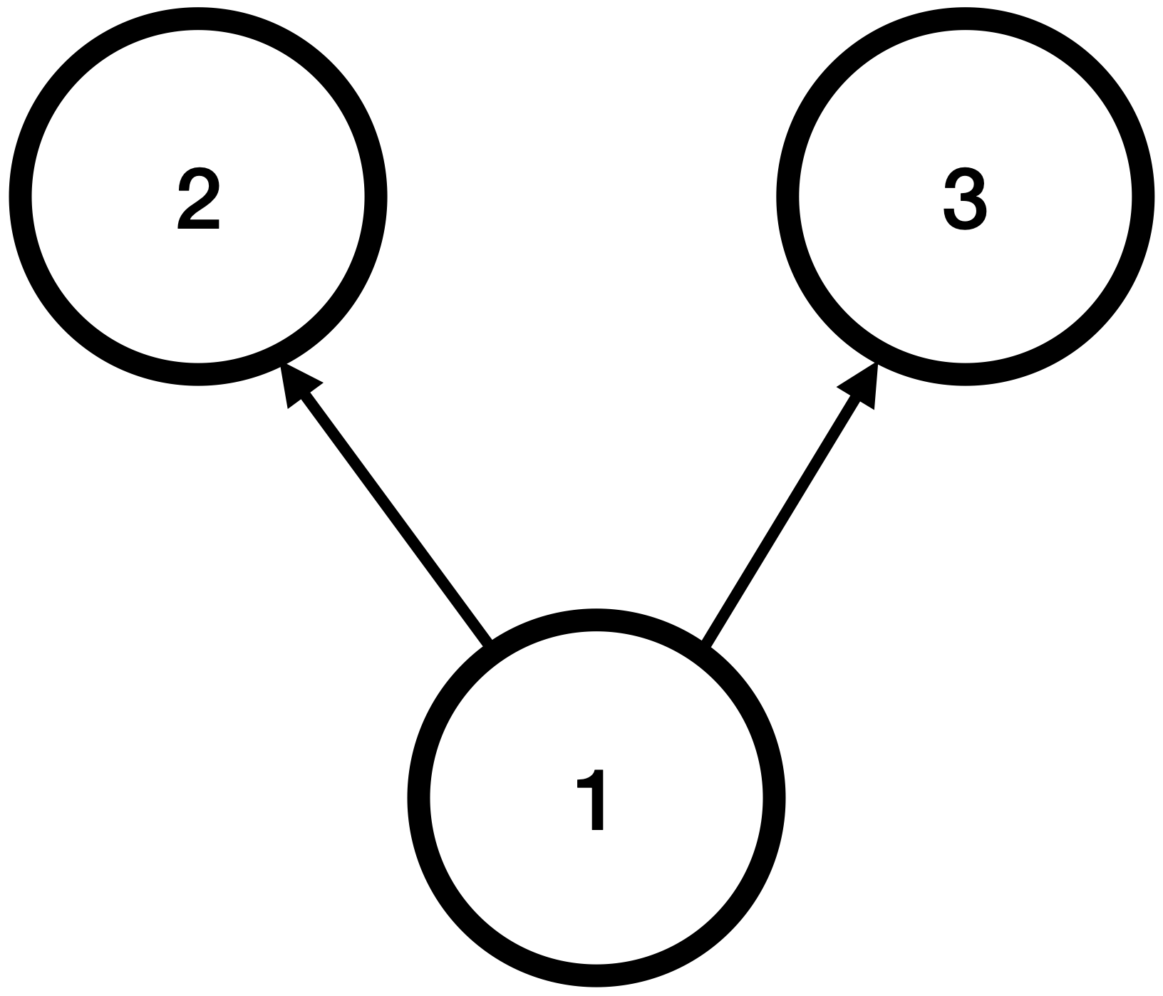
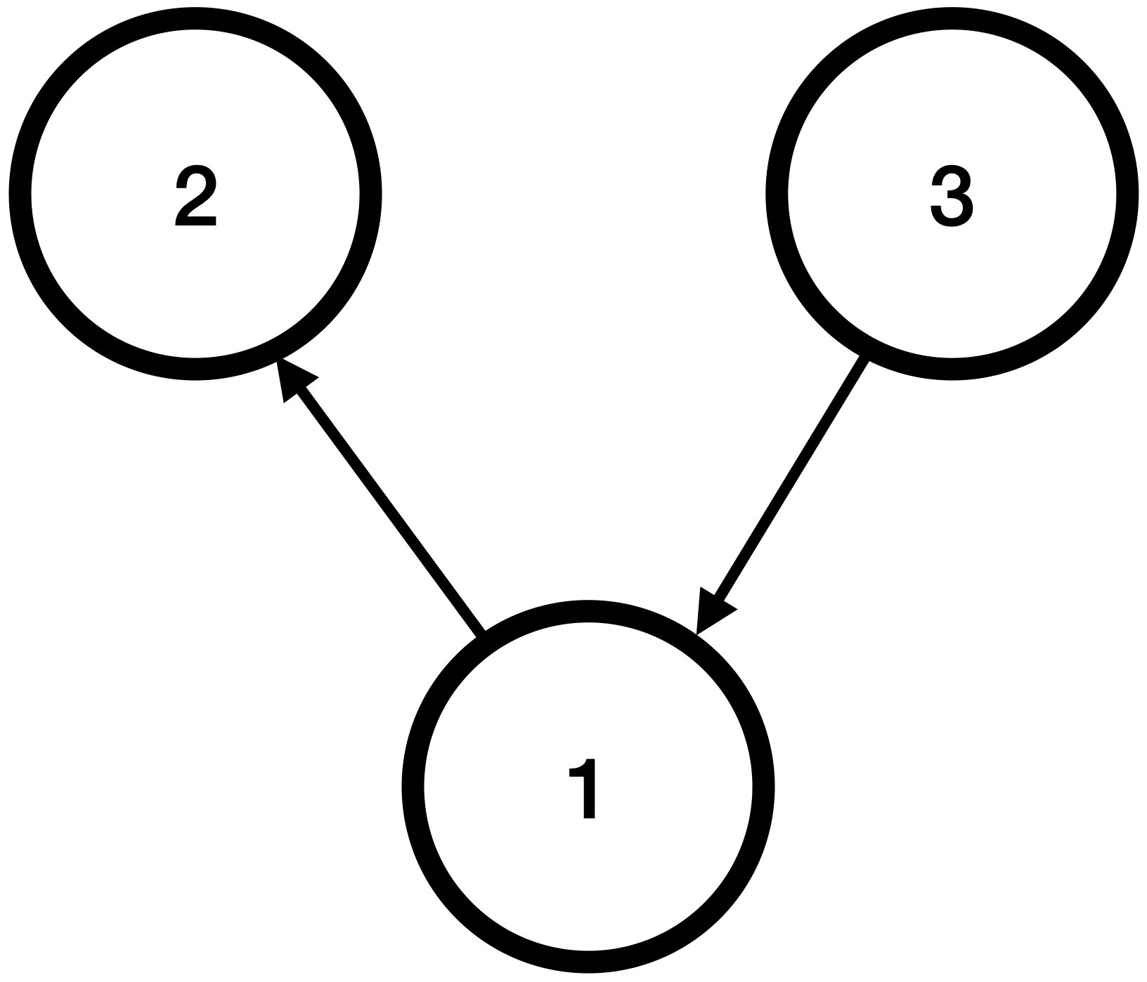
Consider three DAGs depicted in Figure 4. All three DAGs have the same skeleton, none has colliders, and thus they belong to the same equivalence class following Verma and Pearl 1990. Each DAG has three variables, which are all binary, and are generated in the following three ways for the three DAGs, respectively:
for some , . It can be shown that has the same likelihood function, and the three DAGs are not identifiable.
Suppose we test whether there is an edge from to , i.e., we test the hypotheses in (2) with . We first apply the structural learning to estimate the DAG. When the estimated DAG equals , since is not in the ancestor set of , following Step 2b of Algorithm 1, our test returns the -value of 1 directly, and thus would not reject the null hypothesis. When the estimated DAG equals , since the ancestor set of contains , while , the problem becomes testing the marginal independence between and . Following Steps 3 to 6 of Algorithm 1, our test would reject the null, as there is a link from to . When the estimated DAG equals , since the ancestor set of contains both and , and , the problem becomes testing the conditional independence between and given . Again, following Steps 3 to 6 of Algorithm 1, our test would reject the null. In this example, we are not able to differentiate and in the equivalence class from our testing result alone. Even though the testing result is different when the estimated DAG equals , we still do not know if the estimated DAG corresponds to the true DAG in the equivalence class where the data is generated from.
 |
 |
 | ||
Therefore, without specific distributional assumptions, it is generally impossible to distinguish DAGs in an equivalence class, and our test alone cannot either. The main reason is that there is no way to tell if the estimated DAG actually corresponds to the true DAG. Although our test result depends on the estimated DAG, or say, the estimated ordering of the nodes, it is independent of the true DAG that generates the data.
A.5 Extension to non-stationary and time-varying DAG
In Section 2.3, we have focused on the case when DAG is stationary, as imposed by condition (B2). We have also excluded the case when DAG is time-varying, as implied by condition (B3). In this section, we again outline the key steps of extensions, first to non-stationary DAG, then to time-varying DAG. We leave the full investigation as possible future research. To simplify the presentation, we assume . In addition, we denote the random variable at time as , for .
We first consider a non-stationary DAG, and relax the stationarity condition (B2). Toward that end, suppose the DAG structure is piecewise constant over time. That is, there exist some change points, , such that the random vectors are stationary for any . Then, our goal is to test if there exists a directed edge from to , for some .
To test the hypotheses, we first estimate the change point locations and the graph structures given each half of the data. We consider the following optimization,
| (16) | ||||
for all , where denotes the parameters in MLP that models the conditional mean function of when belongs to the time interval , and is a matrix whose th entry equals the Euclidean norm of the th column of . The first penalty in (16) is placed on and is to impose the sparsity structure on the estimated DAG. The second penalty in (16) is placed on , and is to penalize the total number of change points. Dynamic programming method such as Friedrich et al. 2008 can be employed to solve the optimization problem (16). Let denote the estimated change point locations, and denote the estimated graphs, , where denotes the corresponding estimator for . Let denote the set of ancestors of based on , and . We apply Steps 3 to 6 of Algorithm 1 to , and derive the corresponding -value.
We can again show that the above test is consistent. This is based on the following key observation. Under the piecewise stationary structure, the number of change points can be consistently estimated, and the estimated change point locations converge at a faster rate than the estimated DAG. This phenomenon is well-known in the time series literature (Boysen et al. 2009, see e.g.,), where the estimated change point converges at a rate of , and this rate is much faster than the parametric rate. As a consequence, our test is to behave as well as if the true change point locations were known in advance.
Next, we briefly consider a time-varying DAG, which allows to test directed links from past to future observations. Suppose at time , a given node not only depends on other nodes at the same time, but also on past variables at time as well. Our goal is to test if there exists a directed edge from to , for some . We can essentially apply Algorithm 1 to this problem, and can establish the consistency of the test similarly.
Appendix B Additional Results
B.1 Oracle property of the DAG learner
As a by-product of our theoretical analysis, we derive the oracle property of the DAG estimator produced by (9). This result is to guarantee , which was not available in Zheng et al. 2020. It implies that the ordering of the true DAG can be consistently estimated, which in turn ensures the validity of (C1). In this section, for simplicity, we assume the DAG dimension is fixed. Nevertheless, we can extend our proof to the high-dimensional setting in a relatively straightforward fashion, by imposing a certain Hölder smoothness assumption on ; see, e.g., Farrell et al. 2021.
We first define the oracle estimator. For an ordering for a given DAG, consider the estimator , where each is obtained by
where means that, for any that does not belong to this set, the th column of equals zero. In other words, the estimator is computed as if the order were known in advance.
Next, let denote the set of all true orderings. This means, for any true ordering , , for any . In other words, the parents of each node should appear before the occurrence of this node under . It is also worth mentioning that, the true ordering is not necessarily unique, even though the underlying DAG is unique. For instance, consider Example 4 with a v-structure as shown in Figure 1(a). In this example, both and are the true orderings, as there are no directional edges between nodes and .
Next, we introduce some additional conditions. For any ordering , define a least squares loss function, . Moreover, we focus on neural networks with a ReLU activation function, .
- (C5)
All minimizers of are contained in .
- (C6)
The widths of all layers in the MLP share a common asymptotic order . Besides, the number of layers and the asymptotic order diverge with , in that , for some constant .
- (C7)
Suppose MLP is bounded for any .
Condition (C5) is reasonable and holds in numerous scenarios. One example is when all the random errors in model (1) are normally distributed with equal variance. In that case, the least squares loss is proportional to the expected value of the log-likelihood of . Since the underlying DAG is identifiable, any ordering that minimizes the expected log-likelihood belongs to . Condition (C6) is also mild, as both and are the parameters that we specify. The part that ensures that the stochastic error resulting from the parameter estimation in the MLP is negligible. Condition (C7) ensures that the optimizer would not diverge in the sense. Similar assumptions are common in the literature to derive the convergence rates of deep learning estimators (Farrell et al. 2021, see e.g.).
Now we show that the estimator obtained from (9) satisfies the oracle property, i.e., , for some . In other words, is computed as if one of the true ordering were known in advance. By the definition of , Condition (C1) holds for our estimated DAG. Moreover, we note that the oracle property does not imply the selection consistency, i.e., , nor the sure screening property, in that , for any .
Theorem 4.
Suppose in model (1) are a set of continuous functions, (C5)-(C7) hold, the -mixing coefficient in (C4) decays exponentially with , and . Then, with probability approaching one, , for some , as either or .
B.2 Sample splitting
We employ the data splitting and cross-fitting strategy for our test, and use a binary-split in Section 3. To mitigate sample randomization arising from a single binary-split, in this section, we develop a version of our test based on multiple binary-splits. The main idea is to apply the binary-split in Algorithm 1 multiple times, then combine the -values from all splits. In addition, we may also adopt the multi-split strategy of Romano and DiCiccio 2019. These modifications may help reduce the sampling randomization, and may potentially improve the power of the test, but also come with a price of increased computations. Specifically, we carry out the binary-split times. For the th binary-split, we randomly split all samples into two disjoint subsets of equal sizes. We then apply Algorithm 1 to compute the -values, and , respectively, for each half of the data. We next combine these -values by,
where is a constant, and is the empirical -quantile. We recommend to set to a small value, such as or . This follows a similar idea as Meinshausen et al. 2009.
B.3 Gaussian versus non-Gaussian input noise for GANs
When learning the distribution generator in Section 3.5, we take the Gaussian noise as the input of GANs. One may also use other non-Gaussian noises, e.g., uniformly distributed random vectors over a unit hypercube. In general, the performance of the generator computed via GANs is not overly sensitive to the choice of the distribution of the input noise. This is partly because, the objective of the GAN step is to learn a generator , such that the conditional distribution of given can be well approximated by that of given , where is the Gaussian noise. Suppose we use some non-Gaussian noise with the same dimension. Under some regularity conditions, there exists a transformation function , such that has the same distribution as . Define . Then, has the same smoothness properties as . As such, the estimated distribution generator for is expected to have similar statistical properties as that for (Chen et al. 2020).
| Edge | ||||||
|---|---|---|---|---|---|---|
| Hypothesis | ||||||
| Input Noise | Normal | Uniform | Normal | Uniform | Normal | Uniform |
| 0.050 | 0.046 | 0.012 | 0.022 | 0.016 | 0.016 | |
| 0.078 | 0.078 | 0.032 | 0.046 | 0.032 | 0.022 | |
| Edge | ||||||
| Hypothesis | ||||||
| Input Noise | Normal | Uniform | Normal | Uniform | Normal | Uniform |
| 0.014 | 0.020 | 0.032 | 0.030 | 0.030 | 0.034 | |
| 0.030 | 0.032 | 0.058 | 0.052 | 0.046 | 0.052 | |
| Edge | ||||||
| Hypothesis | ||||||
| Input Noise | Normal | Uniform | Normal | Uniform | Normal | Uniform |
| 0.534 | 0.524 | 0.992 | 0.992 | 0.550 | 0.550 | |
| 0.546 | 0.552 | 0.992 | 0.992 | 0.550 | 0.550 | |
| Edge | ||||||
| Hypothesis | ||||||
| Input Noise | Normal | Uniform | Normal | Uniform | Normal | Uniform |
| 0.946 | 0.952 | 0.808 | 0.824 | 0.670 | 0.670 | |
| 0.948 | 0.954 | 0.816 | 0.832 | 0.672 | 0.670 | |
We also conduct a simulation to examine the empirical performance of our test under two distributions, Gaussian and uniform, for the input noise. We adopt the nonlinear model (12) in Section 5, with . Table 2 reports the empirical size and power, i.e., the percentage of times out of 500 data replications when the -value is smaller than the nominal level and , respectively, for some pairs of nodes. It is clearly seen from the table that the results are very similar for two input noise distributions.
B.4 Condition (C1)
To establish the consistency of the proposed test, we require the initial DAG estimator can estimate the ordering consistently; see condition (C1) in Section 4. However, even when (C1) does not hold, our proposed test may still control the type-I error. Actually, in our simulation examples in Section 5, (C1) does not alway hold. Table 3 reports the percentage of times out of 500 data replications when (C1) holds for those selected nodes reported in Table 2 for the nonlinear model (12). It is seen that, for numerous nodes, (C1) only holds for a small fraction of times.
| Nonlinear model (12) with | |||||
| Node | 35 | 40 | 45 | 50 | |
| Percentage | 11.6% | 44.0% | 16.4 % | 2.2% | |
| Nonlinear model (12) with | |||||
| Node | 80 | 85 | 90 | ||
| Percentage | 48 % | 1.9 % | 0 % | ||
| Nonlinear model (12) with | |||||
| Node | 132 | 135 | 137 | 140 | |
| Percentage | 37.1% | 20.0% | 46.5 % | 91.8% | |
B.5 Power comparison
To compare the power of the two testing methods, we further report the empirical power of our SUGAR method minus that of DRT in Figure 5. It is seen that SUGAR achieves generally a higher power than DRT, over 75% of the times in all scenarios.
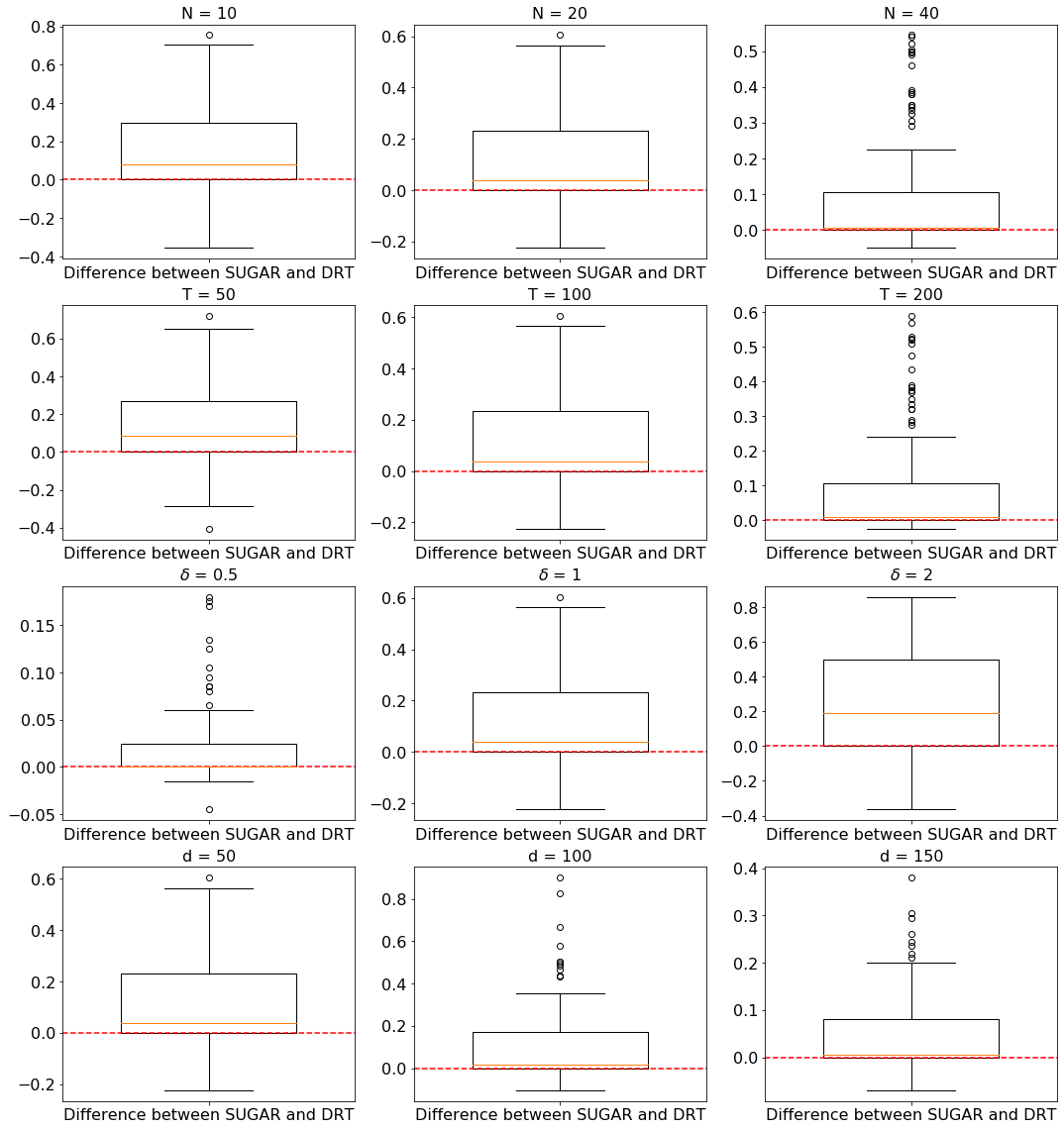
Appendix C Proofs
We present the technical proofs of Proposition 1, Theorems 1, 2 and 3, followed by an auxiliary lemma needed for the proof of Theorem 3. To simplify the notation, we use to denote the data subset throughout this section.
C.1 Proof of Proposition 1
We first show that implies . Under model (1), it follows from Theorem 1.4.1 of Pearl 2009 that the joint distribution of is Markov with respect to the graph. This suggests that the -separation implies the conditional independence (Pearl 2009). Under , and are -separated by . Under the given conditions on , we obtain that and are -separated by as well. Consequently, holds.
We next show that implies . Under , we have . Since and , the additive noise is independent of and . Under model (1), we obtain that . Since , we have . Consequently, we have . As such, we have . Otherwise, there would exist two structural equation models with different graphs that lead to the same joint distribution of , and the identifiability condition would have been violated. Therefore, holds.
This completes the proof of Proposition 1.
C.2 Proof of Theorem 1
It suffices to show that the null hypothesis in (2) is sufficient and necessary to for all square integrable functions .
The sufficiency follows immediately from Proposition 1 and the definition of the conditional independence.
To prove the necessity, it suffices to show there exists some function such that under . Since has a finite second moment, it follows from model (1) and Jensen’s inequality that is also finite. Define the function, . It follows that is square integrable. Also by definition,
This measure is not zero. Otherwise, we would have , which would further imply that the data can be generated by another structural equation model such that is not a direct cause of . This would have violated the identifiability condition.
This completes the proof of Theorem 1.
C.3 Proof of Theorem 2
We begin with a definition. Define
Note that , where
Condition (C1) implies that the set meets the conditions of Proposition 1.
We next divide the proof of this theorem into 6 steps. In Steps 1 to 3, we show that , for , respectively. In Step 4, we show that, conditional on ,
| (17) |
In Step 5, we show that the batched mean estimator converges to the standard deviation of given and the indices of the data subsets . This together with Step 4 yields that given , and . Hence, converges to a standard normal distribution unconditionally as well. In Step 6, we put all the above results together to complete the proof. In the following, we assume the data is fixed. The expectation and variance are taken with respect to the data conditional on .
Step 1. We first use Berbee’s coupling lemma (Dedecker and Louhichi 2002, Lemma 4.1) to approximate by a sum of independent random variables. We then derive the convergence rate of . Since we assume the data is fixed, the index is fixed as well.
Denote and . Consider the sequence formed by , such that for any . By Condition (C3), each sequence is exponentially -mixing, and so is . Following the discussion after Lemma 4.1 of Dedecker and Louhichi 2002, we can construct a sequence of random vectors , such that, with probability at least ,
for any , where we use to denote , and that the sequences and are i.i.d., with .
Let , we have
with probability , where
for . We next bound and , respectively.
For , since is bounded, we have that,
The expectation of the above random variable is of the order . Consequently, .
For , without loss of generality, suppose is divisible by two. By construction,
where each of the above two terms corresponds to a sum of independent random variables. Since the data observations are stationary, it follows from Chebyshev’s inequality that these two terms can be upper bounded by . Next, it suffices to bound the variance term .
By Cauchy-Schwarz inequality, we have
Under and model (1), the residual is independent of the variables on the second line. Consequently,
where denotes some positive constant. Since
By the boundedness of and that is proportional to , the second line is of the order . The third line is of the order under (C2). Without loss of generality, suppose . It follows that . Consequently, .
Putting together the bounds for and , we have that,
with probability at least . Since , set to be proportional to . It then follows that . In addition, since , we obtain . This completes Step 1.
Step 2. This step is derived similarly as Step 1, and the details are omitted.
Step 3. Following similar arguments as in Step 1, we can show that
It then suffices to show , or equivalently, , where
By Cauchy-Schwarz inequality, we have that,
where the first term on the right-hand-side is by condition (C2), and the second term is by condition (C2). Since , we have . This completes Step 3.
Step 4. In this step, we aim to establish (17) for under the bidirectional asymptotic framework. Conditional on the data , the index is fixed. We next show that (17) holds under two scenarios, one with bounded, and the other with diverging.
Scenario 4.1: is bounded and . Condition (C3) implies that each is strong mixing. Since has the bounded fourth moment, and is a bounded function class, it follows from (Rio 2013, Equation (1.12b)) that , with respect to . Since and , it follows that decays at the rate of for some . Consequently,
| (18) |
For each , the process meets the requirements of Theorem 3 in Kourogenis and Pittis 2011. Consequently, for each ,
| (19) |
Since the processes are i.i.d., we have,
Since is bounded, it follows from (19) that
for any . This completes the proof for this scenario.
Scenario 4.2: . We apply the Lindeberg central limit theorem for triangle arrays to derive our results. It suffices to verify the Lindeberg’s condition, i.e.,
for any , where denotes the indicator function.
Under the conditions of Theorem 2, we have that,
| (20) |
with probability tending to . By (20), and that , are identically distributed, it suffices to show
for any , or equivalently,
By (18), we have . By the dominated convergence theorem, it suffices to show
or equivalently,
| (21) |
By Chebyshev’s inequality, (21) holds, because
as diverges to infinity. This completes Step 4.
Step 5. In this step, we establish the consistency of the batched mean estimator. We consider three scenarios, when is bounded and , when is bounded and , and when both .
Scenario 5.1: is bounded and . Note that
Following similar arguments as in Step 4, we can show that
Since , we have . Consequently, it suffices to show that
| (22) |
Since is bounded and , we have . Without loss of generality, suppose is divisible by 2. Following similar arguments as in Step 1, we approximate by
with probability tending to , where denotes the version of such that are independent across different pairs for any . By condition (C3), using the weak law of large numbers, converge in probability to
| (23) |
Similar to (18), we can show that both the right-hand-side of (23) and are bounded. In addition, their difference is asymptotically negligible as and increases to infinity. This yields (22), and completes the proof for this scenario.
Scenario 5.2: is bounded and . By condition (C4), we have under this setting. Then is nearly unbiased to the variance of . The consistency follows from the law of large numbers. This completes the proof for this scenario.
Scenario 5.3: Both and diverge to infinity. It suffices to show (22). Since diverges to infinity, converges to
Following similar arguments as in Scenario 5.1, we can show (22) holds. This completes Step 5.
Step 6. Putting together the results that , , we obtain that . Following similar arguments, we can show that
By (20), we have that,
Note that, under , . By Step 4, we have that, conditional on , (17) holds. Since the limiting distribution is independent to the data , (17) also holds unconditionally. By Step 5, we have that is consistent to the conditional variance of . As and are asymptotically negligible, we can show that is consistent to the conditional variance of as well. By Slutsky’s theorem, we have that,
or equivalently, . This completes the proof of Theorem 2.
C.4 Proof of Theorem 3
We first introduce the notion of the VC type class (Chernozhukov et al. 2014, Definition 2.1). Specifically, let denote a class of measurable functions, with a measurable envelope function such that . For any probability measure , let denote a semi-metric on such that . An -net of the space is a subset of , such that for every , there exists some satisfying . We say that is a VC type class with envelope , if there exist constants , such that , for all , where the supremum is taken over all finitely discrete probability measures on the support of , and is the infimum of the cardinality of -nets of . We refer to as the VC index of .
We next present the proof. Throughout the proof, we assume the indices of the data subsets and are fixed, and show the -value converges to in probability, given and . As such, unconditionally, the -value converges to in probability as well. We begin with a definition,
where is as defined in the proof of Theorem 2. Note that depends on only through the set . Thus, we use the notation to denote . For a given set , define
We next divide the proof of this theorem into 5 steps. In Steps 1 to 3, we show that for , respectively, where denotes the class of subsets that meets the requirements of Proposition 1. In Step 4, we show that
| (24) |
with probability approaching one. In Step 5, we put all the above results together to complete the proof.
Step 1. It suffices to show for any . To simplify the presentation, when there is no confusion, we write and as and , respectively.
To bound , we apply Lemma 1 (see Section C.6). Note that can be written as . Note that the generator belongs to a VC type class with a bounded envelop function . Define the function,
where are i.i.d., and are independent of the observed data. Therefore,
By Lemma A.6 of Chernozhukov et al. 2014, for each , we can show the class of functions corresponds to a VC type class with envelop function uniformly bounded by , where denotes some positive constant. In addition, we have under the given conditions. By setting with some proper choice of , it follows from the auxiliary Lemma 1 given in Section C.6, and the given condition on the VC index that, we have, with probability at least ,
where .
By Bonferroni’s inequality and the condition that ,
The last inequality is due to the fact that, each is standard normal, and , therefore, . This yields that , which completes Step 1.
Step 2. This step is derived similarly as Step 1, and the details are omitted
Step 3. Similar to Step 1, it suffices to bound for each . By Cauchy-Schwarz inequality and following similar arguments as in the proof of Theorem 3 of Shi et al. 2020, we have, up to some logarithmic terms,
Under the condition that , we obtain that for each , which completes Step 3.
Step 4. Based on the results from Steps 1-3, we obtain that
In the proof of Theorem 2, we have shown that . Since depends on only though , we obtain that, with probability approaching one,
| (25) |
Following similar arguments as in the proof of the first three steps, we can show that
Therefore, . It then follows that,
| (26) |
Following similar arguments as in Step 1, we can show that . This together with (25) and (26) yields that,
| (27) |
Next, since , there exists some , such that one of the following two inequalities hold, , or
. Without loss of generality, suppose the former holds.
Note that the objective function is Lipschitz continuous in , and any within the interval satisfies that
Since each is normally distributed, the probability that falls into this interval is lower bounded by for some constant . Since we randomly generate many , the probability that at least one of the falls into this interval is lower bounded by
The above probability tends to under the condition that for some . Consequently, we obtain that,
This together with (25) yields that
By (27), we have that,
By definition, we have that,
Using (27) again, we obtain that,
Step 5. Following similar arguments as in the proof of Steps 1-3 in Theorem 2, we can show that . By (24), we have with probability approaching one. Following similar arguments as in the proof of Theorem 2, we have that . Therefore, diverges to infinity with probability approaching one. Consequently, we obtain that for each . This completes the proof of Theorem 3.
C.5 Proof of Theorem 4
Under the acyclicity constraint in (9), we have for some ordering . We aim to show with probability approaching one.
For any ordering , define the objective function,
where the minimum is taken over all square integrable functions, and the function equals zero almost surely. It is straightforward to show that , where
Let , where is the penalized least squares objective,
Note that, any ordering that minimizes the objective function belongs to . As such, there exists some , such that
| (28) |
We next divide the proof of this theorem into 2 steps. In Step 1, we show that converges to for all . In Step 2, we show that for all , which ultimately leads to the conclusion of this theorem. Note that the DAG dimension is fixed in our proof.
Step 1. It suffices to show , or equivalently, for all , , and any sufficiently small .
Fix an . Since is continuous, it follows from Stone-Weierstrass theorem that there exists a multivariate polynomial function such that the absolute value of the residual is uniformly bounded by . Since , can be written as a function of .
By Theorem 1 of Yarotsky 2017, there exists a feedforward neural network with a bounded number of hidden units that uniformly approximates , with the approximation error uniformly bounded by in absolute value. By Lemma 1 of Farrell et al. 2021, such a feedforward network can be embedded into an MLP with a bounded number of hidden units. Since we allow and to diverge, such an MLP can be further embedded into an MLP with layers and the widths of all layers being proportional to . Denote this MLP by MLP∗, let denote the weight matrices at each layer, and the corresponding bias vectors. We can embed MLP∗ into another MLP, with layers, by setting and for , such that its submatrix formed by columns in and rows in is set to an identity matrix and other entries are set to zero, and to a zero vector. The resulting MLP satisfies , which is finite. Therefore, can be approximated by an MLP with finite such that the approximation error is uniformly bounded by in absolute value. In addition, its weight matrix in the first layer satisfies that . In other words, there exists some , such that
| (29) |
almost surely, and that
| (30) |
It follows from (29) that
This together with (30) and the condition yields that,
By definition, we have that,
It follows that,
To show , it suffices to show that,
Under the conditions of the theorem, we can further restrict the parameter space to the class of , such that is bounded by some constant. As such, the above is upper bounded by
| (31) |
where the supremum is taken over all such that is bounded by some constant. It then suffices to show that (31) is . Following Step 1 of Theorem 2, we can first approximate (31) by a sum of independent random variables. This allows us to upper bounded (31) by many Radamacher complexity terms, under the exponential -mixing condition. Following similar arguments as in Section A.2.2 of Liang 2018, each of these Radamacher complexity terms can be upper bounded by for some , under the given conditions on and . This completes Step 1.
Step 2. Following similar arguments as in Step 1, we can show that
for any and . Since the penalty term is non-negative, and the first term on the right-hand-side is lower bounded by , we obtain that,
for any and .
C.6 An auxiliary lemma
We present a useful lemma that is needed in Step 1 of the proof of Theorem 3. We first briefly introduce the setup. Let be a stationary -mixing process with the -mixing coefficient . Let be a pointwise measurable class of functions that take as input, and has a measurable envelope function . For any , suppose . Let be a positive constant, such that . In the next lemma, we provide an exponential inequality for the empirical process .
Lemma 1.
Suppose the envelop function is uniformly bounded by some constant . In addition, suppose belongs to the class of VC-type class such that for some . Then there exist some constants , such that
for any and .
Proof: We divide the proof of this lemma into three steps. In Step 1, we use Berbee’s coupling lemma (Dedecker and Louhichi 2002, see Lemma 4.1 in) to approximate by the sum of i.i.d. variables. In Step 2, we apply the tail inequality in Lemma 1 of Adamczak 2008 to bound the deviation between the empirical process and its mean. In Step 3, we apply the maximal inequality in Corollary 5.1 of Chernozhukov et al. 2014 to bound the expectation of the empirical process.
Step 1. Following the discussion below Lemma 4.1 of Dedecker and Louhichi 2002, we can construct a sequence of random variables , such that
| (32) |
with probability at least , and that the sequences and are i.i.d., with .
Recall that , we have
Under the boundedness assumption on , the second term on the right-hand-side is bounded from above by . Without loss of generality, suppose is an even number. The first term on the right-hand-side can be bounded from above by . Therefore,
This, together with (32), yields that,
| (33) |
for any . By Bonferroni’s inequality, we obtain that,
for any . Since the process is stationary, we obtain that,
Combining this with (33) yields that,
| (34) | ||||
By construction, are i.i.d. This completes Step 1.
Step 2. Next, we relate the empirical process to its expectation. Without loss of generality, suppose for some integer . Set the constants and in Lemma 1 of Adamczak 2008 to 1, we have that,
for some constant . Combining this with (34), we obtain that,
| (35) | ||||
for any . This completes Step 2.
Step 3. It remains to bound . By Corollary 5.1 of Chernozhukov et al. 2014, we have that,
Combining this with (35), we obtain that,
for some constants , and any . This completes the proof of Lemma 1.