Next-to-Next-to-Leading-Order QCD Prediction for the Photon-Pion Form FactorPreprint: SI-HEP-2021-16, P3H-21-036
Abstract
We accomplish the complete two-loop computation of the leading-twist contribution
to the photon-pion transition form factor
by applying the hard-collinear factorization theorem together with modern multi-loop techniques.
The resulting predictions for the form factor
indicate that the two-loop perturbative correction
is numerically important.
We also demonstrate that our results will play a key role
in disentangling various models of the twist-two pion distribution amplitude
thanks to the envisaged precision at Belle II.
Keywords: Hard exclusive processes, multi-loop computations, pion distribution amplitudes
I introduction
It is widely accepted that the exclusive two-photon production of a light pseudoscalar meson is of utmost importance for probing the partonic landscape of composite hadrons with unprecedented precision and for deepening our understanding of the factorization properties of hard exclusive QCD reactions in general. Historically, the photon-pion transition form factor (TFF) had been explored intensively (see, for instance Cornwall 1966; Gross and Treiman 1971; Brodsky et al. 1971) even before the advent of QCD due to its apparent connection to the axial anomaly Adler 1969; Bell and Jackiw 1969; Bardeen 1969 when taking the vanishing virtuality limits for the two photons. Likewise, for the energetic photo-production at the light-like distance, the dynamical behavior of the TFF can be predicted by applying the operator-product-expansion (OPE) technique for the time-ordered product of two electromagnetic currents Lepage and Brodsky 1979; Lepage and Brodsky 1980. The appearing correlation function with the distinct kinematic set-up concurrently provides the theory description of a variety of two-photon processes including deeply inelastic lepton-hadron scattering (DIS) Feynman 1969; Bjorken 1969; Bjorken and Paschos 1969 and deeply virtual Compton scattering (DVCS) Müller et al. 1994; Ji 1997; Radyushkin 1996, whose importance in establishing QCD as the theory of strong interactions and in accessing the transverse-distance structure of the target hadron cannot be exaggerated (see, for instance Gross 1975; Collins 2013; Dudek et al. 2012; Accardi et al. 2016). In particular, the double-virtual photon-to-pion form factor has been demonstrated to be an indispensable ingredient for determining the hadronic light-by-light scattering (HLbL) contribution to the anomalous magnetic moment of the muon in the dispersive framework Colangelo et al. 2014. The comprehensive data-driven strategy of determining the pion-pole contribution to the HLBL scattering further illustrates that the yielding hadronic uncertainties of can be reduced substantially with the improved determination of the single-virtual photon-pion form factor Hoferichter et al. 2018a; Hoferichter et al. 2018b. Moreover, the collinear QCD dynamics dictating the TFF at large momentum transfer is encapsulated in the universal light-cone distribution amplitude (DA), which is undoubtedly of decisive importance for the model-independent description of semileptonic and nonleptonic -meson decays, such as , and , on the basis of QCD factorization demanding the detailed information on the very pion DA as the fundamental non-perturbative input Beneke and Feldmann 2001; Beneke and Feldmann 2004; Beneke et al. 2005; Beneke et al. 2001. Additionally, the lattice QCD technique has been applied to address the photon-pion form factor at low photon virtualities with very encouraging predictions Gérardin et al. 2016; Gérardin et al. 2019.
Experimentally, the pion TFF with one on-shell and one off-shell photon turns out to be more accessible from the “single-tagged” measurements of the differential cross section Gronberg et al. 1998; Aubert et al. 2009; Uehara et al. 2012. The unexpected scaling violation of the TFF reported by the BaBar measurements Aubert et al. 2009 triggered a storm of enthusiasm in the theory community with diverse speculations from both perturbative and non-perturbative QCD perspectives. The subsequent Belle data Uehara et al. 2012 covering the same kinematical region (where stands for the virtuality of the off-shell photon), however, did not reveal the pronounced increase of the pion TFF in the high- region thus creating a moderate tension at the level of in comparison with the BaBar results. The substantial improvement on the integrated luminosity and the trigger efficiency of the Belle II experiment at SuperKEKB Altmannshofer et al. 2019 will evidently enable a clarification of the observed discrepancy between the BaBar and the Belle data and urgently demand the high-precision theory computation of the TFF in QCD.
At leading power (LP) in the photon-pion TFF can be expressed in terms of the perturbatively calculable coefficient function (CF) and the twist-two pion DA Lepage and Brodsky 1980 (see also Li and Sterman 1992; Musatov and Radyushkin 1997; Li et al. 2014). The short-distance CF at the next-to-leading order (NLO) in had been determined more than three decades ago del Aguila and Chase 1981; Braaten 1983; Kadantseva et al. 1986. The next-to-next-to-leading-order (NNLO) computation of the perturbative matching coefficient was further carried out in the large- approximation Melic et al. 2002 and in the so-called conformal scheme Melic et al. 2003. Consequently, the factorization-scale invariance of the resulting expression for the pion TFF was not achieved in the modified minimal subtraction () scheme at two loops. Accomplishing the full NNLO QCD prediction to the TFF is therefore of the top priority, on the one hand, for developing the perturbative factorization formalism of hard exclusive reactions; and on the other hand, for elevating our capability to confront the yielding theory predictions with the forthcoming precision of Belle II measurements. In this Letter, we will take advantage of the QCD factorization program to obtain analytically the two-loop hard function by evaluating an appropriate bare QCD matrix element at by means of dedicated multi-loop computational strategies and by implementing the ultraviolet (UV) renormalization and the infrared (IR) subtractions, with an exploratory phenomenological analysis regarding the numerical significance of the predicted TFF.
II The photon-pion form factor
We first set up the theory framework for establishing the hard-collinear factorization formula of the TFF . The latter is defined in terms of the matrix element of the electromagnetic current
| (1) |
between an on-shell photon with momentum and a pion with momentum
| (2) |
where refers to the transfer momentum, is the polarization vector of the on-shell photon, and denotes the electric charge of the quark field in units of (the positron charge). Moreover, we have employed the convention and the notation . Introducing further two light-cone vectors and with and allows for the decomposition and .
Applying the hard-collinear factorization theorem results in the LP contribution to the form factor
| (3) |
where the pion decay constant is determined from the experimental measurement Zyla et al. 2020 and represents the factorization scale for which we tacitly adopt in (3). Here the wavefunction with exact isospin symmetry is employed. The CF can be expanded perturbatively in the form (similarly for any other partonic quantity)
| (4) |
The twist-two pion DA is defined by the renormalized matrix element on the light-cone
| (5) |
where is the Wilson line to ensure gauge invariance. We also note that due to charge symmetry, where . The corresponding renormalization group (RG) equation at one loop Efremov and Radyushkin 1980; Lepage and Brodsky 1980 implies the series expansion of in terms of Gegenbauer polynomials,
| (6) |
with the vanishing odd-moments .
It is convenient to evaluate the CF by inspecting the following correlation function
| (7) |
which can be parameterized by the two form factors for the bilinear quark currents with the spin structures Wang and Shen 2017
| (8) |
thanks to the QED Ward identity and charge symmetry. The perpendicular component of any four-vector is defined by . We will dedicate the next section to the two-loop calculation of the bare quantity and subsequently derive the master formula for the CF in (3).
III Two-loop calculation
The techniques entering the calculation of the bare two-loop amplitude have become standard in contemporary multi-loop computations. We first generate the Feynman diagrams with both Feynarts Hahn 2001 and by means of an in-house routine. Sample diagrams are shown in Fig. 1. After taking into account that certain diagrams have color factor zero, vanish due to the Furry theorem and/or represent the flavor-singlet contributions, a set of diagrams (plus the ones with the two photons exchanged) has to be computed. The entire calculation is carried out in dimensional regularization with .
The Dirac and tensor reductions are performed with in-house routines, yielding two-loop scalar integrals, which get further processed with FIRE Smirnov 2008, an implementation of Laporta’s algorithm Laporta and Remiddi 1996; Laporta 2000 relying on integration-by-parts identities Chetyrkin and Tkachov 1981; Tkachov 1981. In addition, we exploit the fact that for the quark momenta , which yields relations between integrals based on momentum conservation and enables us to arrive at the minimal set of master integrals. At this stage, additional Dirac structures besides disappear from the sum of all diagrams, making the QED Ward identity and charge symmetry manifest and providing a valuable check of our calculation.
In total, we get independent master integrals, the analytic -expansion of which can be written in terms of harmonic polylogarithms (HPLs) Remiddi and Vermaseren 2000; Maitre 2006; Maitre 2012. We relegate the explicit analytic results of all master integrals to a forthcoming longer write-up.
IV Ultraviolet Renormalization and Infrared Subtractions
We are now prepared to extract the two-loop contribution to by first introducing the operator basis with
| (9) |
where
| (10) |
with and then by exploiting the matching equation
| (11) |
It is evident from the definitions /2 and that is an evanescent operator vanishing at , and the CP-even operator cannot couple to the pseudoscalar state. We therefore encounter a unique physical operator Wang and Shen 2017.
The correlator assumes the following form to all orders in in terms of the tree-level matrix elements of the effective operators
| (12) |
where . Note that, hereafter, we disregard completely due to parity. The expansion of was already given in Eq. (4), and due to scaleless integrals in dimensional regularization the matrix elements of the light-cone operators are expanded as
| (13) | ||||
Sums over repeated indices are understood to run over , is the tree-level matrix element of , and the renormalization constants can be extracted from the Efremov-Radyushkin-Brodsky-Lepage (ERBL) kernel with the one- and two-loop result given in Efremov and Radyushkin 1980; Lepage and Brodsky 1980 and Sarmadi 1984; Dittes and Radyushkin 1984; Katz 1985; Mikhailov and Radyushkin 1985; Belitsky et al. 1999, respectively. Inserting Eqs. (4), (12), and (13) into Eq. (11) and comparing coefficients of at leads to the following “master formula” for the CF at NNLO
| (14) |
All quantities multiplied by a divergent term in (14) must be expanded beyond to correctly capture all finite terms. It remains important to emphasize the role of the evanescent operator in the master formula (14). Despite the vanishing of evanescent operators in four dimensions, their non-vanishing bare matrix element and evanescent-to-physical mixing (captured by Dugan and Grinstein 1991) are crucial for correctly implementing the IR subtraction and establishing the hard-collinear factorization in our -dimensional framework. These steps are necessary in view of the fact that taking the limit does not commute with the hard-collinear factorization for the correlation function (see also Braun et al. 2004; Beneke et al. 2010).
Substituting the newly derived two-loop correction to the hard function, whose explicit expression is given in the supplemental material, into the factorization formula (3) and adopting further the asymptotic pion DA enable us to write down
| (15) | ||||
Generalizing (15) to account for the non-asymptotic correction will give rise to lengthy expressions due to the intricacy of the NNLO CF. Consequently, we will only evaluate such higher moment effect numerically in the phenomenological exploration. In particular, it has been verified explicitly that the photon-pion form factor computed from the factorization formula (3) is independent of the factorization scale at , with the aid of the two-loop evolution equation of the twist-two pion DA Sarmadi 1984; Dittes and Radyushkin 1984; Katz 1985; Mikhailov and Radyushkin 1985; Belitsky et al. 1999. Subsequently, the complete next-to-next-to-leading-logarithmic (NNLL) resummation of appearing in (3) is achieved by virtue of the three-loop evolution equation of in the naive dimensional regularization (NDR) scheme Braun et al. 2017, which is implemented throughout our computation.
V Numerical analysis
We now turn to explore the numerical implications of the achieved NNLL computation of with three phenomenological models of at ,
| (16) | |||||
Model I is inspired from the AdS/QCD correspondence Brodsky and de Teramond 2008 with modifications from the most recent lattice result Bali et al. 2019, which corresponds to . The construction of Model II is achieved by matching the light-cone QCD sum rules of the pion electromagnetic form factor in the space-like region onto the modified dispersion integral of the modulus of the time-like form factor Cheng et al. 2020. The intervals of and in Model III Bakulev et al. 2001; Mikhailov et al. 2016; Stefanis 2020 are determined from the method of QCD sum rules Mikhailov and Radyushkin 1992. To facilitate the implementation of the three-loop evolution of the leading-twist pion DA Braun et al. 2017; Strohmaier 2018, we will apply the Gegenbauer expansion for the “holographic”-type Model I by discarding with (see also Agaev et al. 2011).

Adopting Model I as our default choice, we present in Fig. 2 the resulting impacts of QCD radiative corrections to the TFF at LP as well as the numerical features of the power suppressed terms from the twist-four collinear dynamics of the pion system Khodjamirian 1999 and from the long-distance photon correction Wang and Shen 2017. Inspecting the numerical patterns of the various dynamical mechanisms displayed in Fig. 2 implies that the NNLL twist-two correction can reduce the corresponding NLL prediction by an amount of at (in agreement with the previous estimate Mikhailov et al. 2016), while the genuine one-loop perturbative correction is responsible for a constant reduction of the LL contribution in the same kinematic domain. By contrast, the above-mentioned subleading contributions are observed to bring about the negligible corrections Wang and Shen 2017. The full two-loop computation of the LP effect in the TFF is therefore indeed of extraordinary phenomenological significance. Additionally, the three-loop QCD correction estimated with the “naïve non-Abelianization” prescription Beneke and Braun 1995 is expected to be approximately of the one-loop radiative effect without adding further the systematic uncertainty.
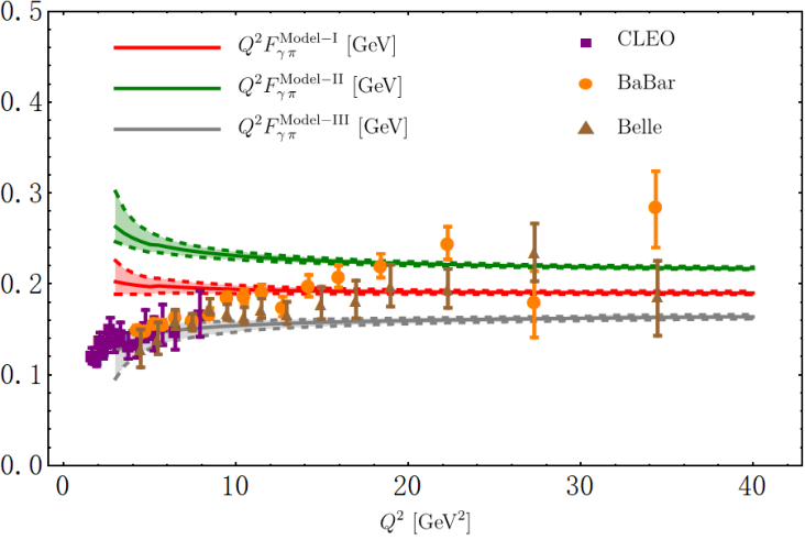
We proceed to present in Fig. 3 the theory predictions of the TFF for the three phenomenological models of the leading-twist pion DA. As the dominating non-perturbative uncertainties of our numerical analysis from can be inferred from the discrepancies of the obtained theoretical results for the distinct sample models, the quoted uncertainties in (16) are not included in the three shaded (red, green, gray) bands in Fig. 3 to highlight the perturbative uncertainty from the variation of with Agaev et al. 2011. The distinctive snapshot of the well-separated uncertainty bands for the three models is particularly encouraging to differentiate numerous speculations on the intricate behaviors of the twist-two pion DA. Furthermore, the theory predictions from the incomplete two-loop computation of in the large approximation differ from our full results by almost a factor of two at high-. Additionally, the NNLL improved hard-collinear factorization tends to validate the scaling behaviour of the photon-pion form factor at with an impressive precision of , which will be confronted with the future Belle II data. As expected, such scaling behaviour is broken down at low momentum transfer, numerically , due to the pronounced subleading power contributions. A more detailed investigation of the asymptotic behaviour of in the hard-collinear factorization framework can be pushed forward by introducing the scaling-rate quantity as proposed in Stefanis 2019; Stefanis 2020.
We finally address the actual impact of the NNLL correction to the photon-pion form factor on the model-independent determination of the twist-two pion DA in anticipation of the upcoming precision Belle II measurements. To this end, we investigate the intrinsic sensitivity of the form factor with regard to the poorly constrained Gegenbauer moment , by employing the improved lattice result for Bali et al. 2019 and by further leaving out the higher moments for illustration purpose. The numerical implication displayed in Fig. 4 reveals that the two-loop computation of the photon-pion TFF is indeed highly beneficial for pinning down the theory uncertainty of the extracted value of (up to a factor of two improvement approximately when compared with the corresponding one-loop result).

VI Conclusions
In summary, we have endeavored to carry out, for the first time, the complete two-loop computation of the leading-twist contribution to the photon-pion form factor in the hard-collinear factorization framework. The phenomenological significance of such higher-order perturbative effect was further addressed by employing the three non-perturbative models of the twist-two pion DA. The genuine correction to the hard matching coefficient was demonstrated to be numerically important at , and in particular, the previously evaluated radiative correction at only accounts for a moderate portion (approximately ) of the full NNLL QCD effect. Moreover, our improved theory predictions of the form factor appear to be promising for better constraining the shape parameters of the pion DA. The established two-loop QCD factorization formula of the photon-pion form factor is then naturally expected to be of notable importance for exploiting the many facets of the strong interaction dynamics embedded in hard exclusive reactions.
Acknowledgements.
Acknowledgements
We would like to thank Ulrich Haisch for useful correspondence, and Vladimir Braun and Alexander Manashov for sharing their results Braun et al. 2021 with us prior to publication. We have found full agreement with their expression for the two-loop coefficient function. Y.J. is also grateful to Alexander Manashov and Goutam Das for illuminating discussions. J.G. is partially supported by the Deutscher Akademischer Austauschdienst (DAAD). The research of T.H. and Y.J. was supported in part by the Deutsche Forschungsgemeinschaft (DFG, German Research Foundation) under grant 396021762 - TRR 257. Y.M.W. acknowledges support from the National Youth Thousand Talents Program, the Youth Hundred Academic Leaders Program of Nankai University, the National Natural Science Foundation of China with Grant No. 11675082, 11735010 and 12075125, and the Natural Science Foundation of Tianjin with Grant No. 19JCJQJC61100.
References
- Cornwall (1966) J. M. Cornwall, Phys. Rev. Lett. 16, 1174 (1966).
- Gross and Treiman (1971) D. J. Gross and S. B. Treiman, Phys. Rev. D 4, 2105 (1971).
- Brodsky et al. (1971) S. J. Brodsky, T. Kinoshita, and H. Terazawa, Phys. Rev. D 4, 1532 (1971).
- Adler (1969) S. L. Adler, Phys. Rev. 177, 2426 (1969).
- Bell and Jackiw (1969) J. S. Bell and R. Jackiw, Nuovo Cim. A 60, 47 (1969).
- Bardeen (1969) W. A. Bardeen, Phys. Rev. 184, 1848 (1969).
- Lepage and Brodsky (1979) G. P. Lepage and S. J. Brodsky, Phys. Lett. B 87, 359 (1979).
- Lepage and Brodsky (1980) G. P. Lepage and S. J. Brodsky, Phys. Rev. D 22, 2157 (1980).
- Feynman (1969) R. P. Feynman, Conf. Proc. C 690905, 237 (1969).
- Bjorken (1969) J. D. Bjorken, Phys. Rev. 179, 1547 (1969).
- Bjorken and Paschos (1969) J. D. Bjorken and E. A. Paschos, Phys. Rev. 185, 1975 (1969).
- Müller et al. (1994) D. Müller, D. Robaschik, B. Geyer, F. M. Dittes, and J. Hořejši, Fortsch. Phys. 42, 101 (1994), arXiv:hep-ph/9812448 .
- Ji (1997) X.-D. Ji, Phys. Rev. D 55, 7114 (1997), arXiv:hep-ph/9609381 .
- Radyushkin (1996) A. V. Radyushkin, Phys. Lett. B 380, 417 (1996), arXiv:hep-ph/9604317 .
- Gross (1975) D. J. Gross, Conf. Proc. C 7507281, 141 (1975).
- Collins (2013) J. Collins, Foundations of perturbative QCD, Vol. 32 (Cambridge University Press, 2013).
- Dudek et al. (2012) J. Dudek et al., Eur. Phys. J. A 48, 187 (2012), arXiv:1208.1244 [hep-ex] .
- Accardi et al. (2016) A. Accardi et al., Eur. Phys. J. A 52, 268 (2016), arXiv:1212.1701 [nucl-ex] .
- Colangelo et al. (2014) G. Colangelo, M. Hoferichter, M. Procura, and P. Stoffer, JHEP 09, 091 (2014), arXiv:1402.7081 [hep-ph] .
- Hoferichter et al. (2018a) M. Hoferichter, B.-L. Hoid, B. Kubis, S. Leupold, and S. P. Schneider, Phys. Rev. Lett. 121, 112002 (2018a), arXiv:1805.01471 [hep-ph] .
- Hoferichter et al. (2018b) M. Hoferichter, B.-L. Hoid, B. Kubis, S. Leupold, and S. P. Schneider, JHEP 10, 141 (2018b), arXiv:1808.04823 [hep-ph] .
- Beneke and Feldmann (2001) M. Beneke and T. Feldmann, Nucl. Phys. B 592, 3 (2001), arXiv:hep-ph/0008255 .
- Beneke and Feldmann (2004) M. Beneke and T. Feldmann, Nucl. Phys. B 685, 249 (2004), arXiv:hep-ph/0311335 .
- Beneke et al. (2005) M. Beneke, T. Feldmann, and D. Seidel, Eur. Phys. J. C 41, 173 (2005), arXiv:hep-ph/0412400 .
- Beneke et al. (2001) M. Beneke, G. Buchalla, M. Neubert, and C. T. Sachrajda, Nucl. Phys. B 606, 245 (2001), arXiv:hep-ph/0104110 .
- Gérardin et al. (2016) A. Gérardin, H. B. Meyer, and A. Nyffeler, Phys. Rev. D 94, 074507 (2016), arXiv:1607.08174 [hep-lat] .
- Gérardin et al. (2019) A. Gérardin, H. B. Meyer, and A. Nyffeler, Phys. Rev. D 100, 034520 (2019), arXiv:1903.09471 [hep-lat] .
- Gronberg et al. (1998) J. Gronberg et al. (CLEO), Phys. Rev. D 57, 33 (1998), arXiv:hep-ex/9707031 .
- Aubert et al. (2009) B. Aubert et al. (BaBar), Phys. Rev. D 80, 052002 (2009), arXiv:0905.4778 [hep-ex] .
- Uehara et al. (2012) S. Uehara et al. (Belle), Phys. Rev. D 86, 092007 (2012), arXiv:1205.3249 [hep-ex] .
- Altmannshofer et al. (2019) W. Altmannshofer et al. (Belle-II), PTEP 2019, 123C01 (2019), [Erratum: PTEP 2020, 029201 (2020)], arXiv:1808.10567 [hep-ex] .
- Li and Sterman (1992) H.-n. Li and G. F. Sterman, Nucl. Phys. B381, 129 (1992).
- Musatov and Radyushkin (1997) I. V. Musatov and A. V. Radyushkin, Phys. Rev. D56, 2713 (1997), arXiv:hep-ph/9702443 [hep-ph] .
- Li et al. (2014) H.-N. Li, Y.-L. Shen, and Y.-M. Wang, JHEP 01, 004 (2014), arXiv:1310.3672 [hep-ph] .
- del Aguila and Chase (1981) F. del Aguila and M. K. Chase, Nucl. Phys. B 193, 517 (1981).
- Braaten (1983) E. Braaten, Phys. Rev. D 28, 524 (1983).
- Kadantseva et al. (1986) E. P. Kadantseva, S. V. Mikhailov, and A. V. Radyushkin, Yad. Fiz. 44, 507 (1986).
- Melic et al. (2002) B. Melic, B. Nizic, and K. Passek, Phys. Rev. D 65, 053020 (2002), arXiv:hep-ph/0107295 .
- Melic et al. (2003) B. Melic, D. Mueller, and K. Passek-Kumericki, Phys. Rev. D 68, 014013 (2003), arXiv:hep-ph/0212346 .
- Zyla et al. (2020) P. A. Zyla et al. (Particle Data Group), PTEP 2020, 083C01 (2020).
- Efremov and Radyushkin (1980) A. V. Efremov and A. V. Radyushkin, Phys. Lett. B 94, 245 (1980).
- Wang and Shen (2017) Y.-M. Wang and Y.-L. Shen, JHEP 12, 037 (2017), arXiv:1706.05680 [hep-ph] .
- Hahn (2001) T. Hahn, Comput. Phys. Commun. 140, 418 (2001), arXiv:hep-ph/0012260 .
- Smirnov (2008) A. V. Smirnov, JHEP 10, 107 (2008), arXiv:0807.3243 [hep-ph] .
- Laporta and Remiddi (1996) S. Laporta and E. Remiddi, Phys. Lett. B 379, 283 (1996), arXiv:hep-ph/9602417 .
- Laporta (2000) S. Laporta, Int. J. Mod. Phys. A 15, 5087 (2000), arXiv:hep-ph/0102033 .
- Chetyrkin and Tkachov (1981) K. G. Chetyrkin and F. V. Tkachov, Nucl. Phys. B 192, 159 (1981).
- Tkachov (1981) F. V. Tkachov, Phys. Lett. B 100, 65 (1981).
- Remiddi and Vermaseren (2000) E. Remiddi and J. A. M. Vermaseren, Int. J. Mod. Phys. A 15, 725 (2000), arXiv:hep-ph/9905237 .
- Maitre (2006) D. Maitre, Comput. Phys. Commun. 174, 222 (2006), arXiv:hep-ph/0507152 .
- Maitre (2012) D. Maitre, Comput. Phys. Commun. 183, 846 (2012), arXiv:hep-ph/0703052 .
- Sarmadi (1984) M. H. Sarmadi, Phys. Lett. B 143, 471 (1984).
- Dittes and Radyushkin (1984) F. M. Dittes and A. V. Radyushkin, Phys. Lett. B 134, 359 (1984).
- Katz (1985) G. R. Katz, Phys. Rev. D 31, 652 (1985).
- Mikhailov and Radyushkin (1985) S. V. Mikhailov and A. V. Radyushkin, Nucl. Phys. B 254, 89 (1985).
- Belitsky et al. (1999) A. V. Belitsky, D. Mueller, and A. Freund, Phys. Lett. B 461, 270 (1999), arXiv:hep-ph/9904477 .
- Dugan and Grinstein (1991) M. J. Dugan and B. Grinstein, Phys. Lett. B 256, 239 (1991).
- Braun et al. (2004) V. M. Braun, D. Y. Ivanov, and G. P. Korchemsky, Phys. Rev. D 69, 034014 (2004), arXiv:hep-ph/0309330 .
- Beneke et al. (2010) M. Beneke, T. Huber, and X.-Q. Li, Nucl. Phys. B832, 109 (2010), arXiv:0911.3655 [hep-ph] .
- Braun et al. (2017) V. M. Braun, A. N. Manashov, S. Moch, and M. Strohmaier, JHEP 06, 037 (2017), arXiv:1703.09532 [hep-ph] .
- Brodsky and de Teramond (2008) S. J. Brodsky and G. F. de Teramond, Phys. Rev. D 77, 056007 (2008), arXiv:0707.3859 [hep-ph] .
- Bali et al. (2019) G. S. Bali, V. M. Braun, S. Bürger, M. Göckeler, M. Gruber, F. Hutzler, P. Korcyl, A. Schäfer, A. Sternbeck, and P. Wein (RQCD), JHEP 08, 065 (2019), [Addendum: JHEP 11, 037 (2020)], arXiv:1903.08038 [hep-lat] .
- Cheng et al. (2020) S. Cheng, A. Khodjamirian, and A. V. Rusov, Phys. Rev. D 102, 074022 (2020), arXiv:2007.05550 [hep-ph] .
- Bakulev et al. (2001) A. P. Bakulev, S. V. Mikhailov, and N. G. Stefanis, Phys. Lett. B 508, 279 (2001), [Erratum: Phys.Lett.B 590, 309–310 (2004)], arXiv:hep-ph/0103119 .
- Mikhailov et al. (2016) S. V. Mikhailov, A. V. Pimikov, and N. G. Stefanis, Phys. Rev. D 93, 114018 (2016), arXiv:1604.06391 [hep-ph] .
- Stefanis (2020) N. G. Stefanis, Phys. Rev. D 102, 034022 (2020), arXiv:2006.10576 [hep-ph] .
- Mikhailov and Radyushkin (1992) S. V. Mikhailov and A. V. Radyushkin, Phys. Rev. D 45, 1754 (1992).
- Strohmaier (2018) M. Strohmaier, Conformal symmetry breaking and evolution equations in Quantum Chromodynamics, Ph.D. thesis, Regensburg U. (2018).
- Agaev et al. (2011) S. S. Agaev, V. M. Braun, N. Offen, and F. A. Porkert, Phys. Rev. D 83, 054020 (2011), arXiv:1012.4671 [hep-ph] .
- Khodjamirian (1999) A. Khodjamirian, Eur. Phys. J. C 6, 477 (1999), arXiv:hep-ph/9712451 .
- Beneke and Braun (1995) M. Beneke and V. M. Braun, Phys. Lett. B 348, 513 (1995), arXiv:hep-ph/9411229 .
- Stefanis (2019) N. G. Stefanis, (2019), arXiv:1904.02631 [hep-ph] .
- Braun et al. (2021) V. M. Braun, A. N. Manashov, S. Moch, and J. Schoenleber, Phys. Rev. D 104, 094007 (2021), arXiv:2106.01437 [hep-ph] .
Supplemental Materials to Next-to-Next-to-Leading-Order QCD Prediction for the Photon-Pion Form Factor
Appendix A Analytic expressions in the -scheme
The master formula (14) was derived under the assumption that dimensional regularization is used on both sides of Eq. (11) for both UV and IR divergences. However, to determine the UV-renormalization constants we apply the following procedure (see e.g. Beneke et al. 2010; Wang and Shen 2017). The renormalized matrix elements of the effective operators are expressed as follows
| (S1) |
and the matrix elements are obtained with dimensional regularization applied only to the UV divergences but with the IR regularization scheme being different from the dimensional one. Renormalizing the matrix elements of the evanescent operator to zero Dugan and Grinstein 1991 yields the relations
| (S2) |
where is IR finite as expected albeit both and are IR divergent.
We now present the explicit expressions of the two-loop hard coefficient function with the NDR scheme of
| (S3) |
where
| (S4) | ||||
| (S5) | ||||
| (S6) | ||||
with . The harmonic polylogarithms (HPLs) are defined recursively by
| (S7) |
The subscript of is called the weight vector. For the weight functions we have , , and , where the latter does not occur in the present calculation. A common abbreviation for the weight vector is to replace occurrences of zero(s) to the left of by . For example, . Moreover, all the HPL functions that we have are representable in the form of simple functions of argument with . Our result for the color structure is in full agreement with Melic et al. 2002. Besides, we note that the terms in (S6) proportional to are reproducible directly from the coefficient function in DIS.