Hydrodynamics of granular gases of inelastic and rough hard disks or spheres. I. Transport coefficients
Abstract
The transport coefficients for dilute granular gases of inelastic and rough hard disks or spheres with constant coefficients of normal () and tangential () restitution are obtained in a unified framework as functions of the number of translational () and rotational () degrees of freedom. The derivation is carried out by means of the Chapman–Enskog method with a Sonine-like approximation in which, in contrast to previous approaches, the reference distribution function for angular velocities does not need to be specified. The well-known case of purely smooth -dimensional particles is recovered by setting and formally taking the limit . In addition, previous results [G. M. Kremer, A. Santos, and V. Garzó, Phys. Rev. E 90, 022205 (2014)] for hard spheres are reobtained by taking , while novel results for hard-disk gases are derived with the choice , . The singular quasismooth limit () and the conservative Pidduck’s gas () are also obtained and discussed.
I Introduction
A granular gas is essentially a system of particles that move erratically and collide inelastically. The simplest model to describe its kinetic behavior consists in a collection of inelastic hard disks (HD) or spheres (HS) with a constant coefficient of normal restitution (with ) Campbell 1990; Pöschel and Luding 2001; Goldhirsch 2003; Brilliantov and Pöschel 2004; Garzó 2019. A plausible improvement of the model is the addition of collisional friction due to surface roughness (as demanded by recent experiments Yu et al. 2020), which can be quantified via a constant coefficient of tangential restitution (with ) Jenkins and Richman 1985.
Certainly, this simple two-parameter model does not account for sliding effects that can be relevant in grazing collisions Foerster et al. 1994. Models with a Coulomb friction constant Walton 1993; Louge are more realistic but less theoretically tractable outside of the quasielastic and/or quasismooth limits Jenkins and Zhang 2002; Goldhirsch et al. 2005a; Goldhirsch et al. 2005b. Therefore, the model for granular fluids, which captures satisfactorily well the basics of collision processes, represents an excellent compromise between simplicity and physical content Brilliantov et al. 2007; Gayen and Alam 2008; Mitrano et al. 2013.
In analogy with a conventional fluid, a hydrodynamic description is also applicable and useful in the case of granular gases McNamara 1993; Goldshtein and Shapiro 1995; Grossman et al. 1997; Sela and Goldhirsch 1998; Dufty 2000; Dufty 2001; Garzó and Dufty 2002; Brilliantov and Pöschel 2003; Goldhirsch et al. 2005b; Serero et al. 2006; Vega Reyes and Urbach 2009; Vega Reyes et al. 2010; Dufty and Brey 2011; Garzó and Santos 2011; Gradenigo et al. 2011a; Gradenigo et al. 2011b; García de Soria et al. 2013; Garzó 2019. If the gas is made of perfectly elastic () and either perfectly smooth () or perfectly rough () hard particles Pidduck 1922, then kinetic energy is conserved upon collisions. Therefore, a complete set of hydrodynamic variables is defined from the densities of the conserved quantities, that is, particle density (reflecting mass conservation), flow velocity (due to momentum conservation), and temperature (associated with energy conservation). However, for inelastic () and/or imperfectly rough () hard particles, energy is no longer preserved at the collisional level. Despite that, temperature is usually included as a hydrodynamic variable Garzó 2019, except that a sink term (the so-called cooling rate) needs to be included in the energy balance equation. Therefore, as done in Refs. Kremer et al. 2014; Garzó et al. 2018 for (three-dimensional) HS, in this paper we will choose as hydrodynamic variables. In contrast, the mean angular velocity is not a collisional invariant, even if , and thus it is not included as a hydrodynamic field in our description.
To the best of our knowledge, the derivation by means of the Chapman–Enskog method of the Navier–Stokes–Fourier (NSF) hydrodynamic description (for generic constant coefficients of restitution and ) of a two-dimensional granular gas of inelastic and rough HD has not been carried out yet. The aim of this work is to fill this gap in an inclusive way by generalizing the study to a hard-particle system with and translational and rotational degrees of freedom, respectively, in analogy with our previous study on the energy production rates in granular mixtures Megías and Santos 2019a; Megías and Santos 2019b. In this way, apart from obtaining the sought results for HD gases with the choice , the results for rough HS Kremer et al. 2014 are recovered by setting . Additionally, the expressions for -dimensional smooth particles () Brey and Cubero 2001 are also reobtained by formally taking .
Whereas the three-dimensional is perhaps the most general, verisimilar, and intuitive geometry, a two-dimensional constrained system is also found in ordinary life, like a set of marbles moving and spinning on a plane or the pucks and strikers in the air hockey game. But the most important asset of the two-dimensional geometry resides in its ordinary use in experiments setups Clement and Rajchenbach 1991; Feitosa and Menon 2002; Painter et al. 2003; Yanpei et al. 2011; Grasselli et al. 2015; Scholz and Pöschel 2017; Grasselli et al. 2017; López-Castaño et al. 2021; López Castaño et al. 2021. Thus, this work aims at providing testable results for the hydrodynamic transport coefficients within a general framework that encompasses the three- and two-dimensional geometries of spinning particles.
The intricacy of the -generalization resides in the difficulties associated with a uniform characterization of the HS and HD vector spaces. The HS case is described by a three-dimensional Euclidean space common to both translational and angular velocities. However, to preserve the two-dimensional confinement of the HD system, angular velocities are orthogonal to the translational ones. To unify both descriptions in a common framework, we will consider the three-dimensional Euclidean space as an embedding space for the translational and angular velocity subspaces. Those subspaces coincide with the embedding space for HS systems, whereas they form an orthogonal decomposition of the vector space in the HD case. Within such a description, all vector operations and relations can be written as in the HS system Megías and Santos 2019b; Megías and Santos 2019a. Although this mathematical description seems to be straightforward, it is rather tricky in some aspects, as will be seen.
The present paper is structured as follows. In Sec. II, the Boltzmann equation framework is established and the balance equations of the hydrodynamic fields, , are derived in terms of and . This mathematical description allows us to introduce in Sec. III the Chapman–Enskog method around the homogeneous cooling state (HCS), from which we obtain the velocity distribution function (VDF) to first order in the hydrodynamic gradients, , under the form of four linear integral equations. To solve those equations, two successive approximations are worked out in Sec. IV. First, a Sonine-like approximation is assumed without prejudicing the form of the zeroth-order HCS VDF ; this allows us to express the NSF transport coefficients in terms of velocity cumulants and collision integrals of . As a second step, the unknown function is approximated by a Maxwellian distribution for the translational velocities times a generic marginal distribution for the angular velocities, what allows us to derive explicit expressions for the transport coefficients (see Table 1 below). The results are illustrated in Sec. V for both spheres and disks, including some interesting limiting situations. Finally, concluding remarks and main results are summed up in Sec. VI.
II Granular gas of inelastic and rough hard particles
II.1 Boltzmann equation
We consider a HD or HS granular gas made of identical particles of diameter , mass , and moment of inertia . The reduced moment of inertia takes the values for uniform disks and for uniform spheres; its maximum value is (HD) and (HS). The translational and angular velocities of a particle will be denoted by and , respectively. Whenever convenient, we will use the short-hand notations and for simplicity.
Particle-particle collisions are characterized by constant coefficients of normal () and tangential () restitution (see Appendix A for a summary of the collision rules). As said in Sec. I, vector relations within our generalized description belongs to an embedding space, namely the three-dimensional Euclidean space . Therefore, the collision rules in Appendix A are presented in the three-dimensional framework.
We will carry out a kinetic-theory description of a dilute granular gas, in the sense that the one-body VDF will be enough to characterize the system. This approach is complemented with the assumption of molecular chaos or Stosszahlansatz. The analytical treatment is then based on the Boltzmann equation in the absence of external forces, which reads
| (1) |
where is the VDF at time and is the Boltzmann bilinear collision operator:
| (2) |
Here, is the relative translational velocity, is the intercenter unit vector at contact, the subscript in the integral over designates the constraint , and and , the double primes denoting precollisional quantities giving rise to unprimed quantities as postcollisional values. Moreover, use has been made of the Jacobian given by (49).
II.2 Hydrodynamic balance equations
From a macroscopic point of view, the flow of a low-density granular gas can be fully described by the knowledge of the following hydrodynamic fields: particle number density , hydrodynamic flow velocity , and total granular temperature . They are given by
| (3a) | |||
| (3b) | |||
| (3c) |
where
| (4) |
being the peculiar velocity. The angular brackets denote averages defined generically as
| (5) |
Note that the rotational temperature is not defined with respect to the mean angular velocity because the latter is not a conserved quantity Kremer et al. 2014.
Given a quantity , its associated transfer equation can be obtained by multiplying both sides of the Boltzmann equation, Eq. (1), by and integrating over translational and angular velocities. The result is
| (6) |
where is the collisional production term of the quantity , given by
| (7) |
Here, the operator acting on a generic quantity yields the difference between the postcollisional and precollisional values of , i.e., .
The balance equations for mass, momentum, and energy are obtained from Eq. (6) by choosing , , , , and . This yields, respectively,
| (8a) | |||
| (8b) | |||
| (8c) | |||
| (8d) | |||
| (8e) |
In these equations, is the material time derivative and is the mass density. Moreover, is the pressure tensor, () is the translational (rotational) contribution to the total heat flux , () is the translational (rotational) energy production rate, and is the cooling rate. These quantities are defined as
| (9a) | |||
| (9b) | |||
| (9c) | |||
| (9d) |
In Eq. (9c), the collisional rates of change and are obtained from Eq. (II.2) by setting and , respectively.
II.3 Homogeneous cooling state
Before analyzing inhomogeneous states in terms of the transport coefficients at the NSF order in Secs. III–V, let us consider the HCS, henceforth represented by the superscript . In that case (), Eqs. (8a) and (8b) yield and , while Eqs. (8c)–(8e) become
| (10a) | |||
| (10b) | |||
| (10c) |
Note that we have not attached a superscript to the global temperature because of its status as a hydrodynamic variable. The Boltzmann equation, Eq. (1), reduces in the HCS to
| (11) |
Since in the HCS all the time-dependence of occurs through a dependence on , we can write Garzó 2019; Kremer et al. 2014
| (12) |
The rotational-to-translational, translational-to-total, and rotational-to-total temperature ratios are defined as
| (13a) | |||
| (13b) |
Those temperature ratios are stationary in the HCS, so that Eqs. (10) imply that .
The exact solution to Eq. (11) is not known, but good estimates for the production rates , , and can be obtained by assuming the simple trial function
| (14) |
where
| (15) |
are the translational and rotational thermal velocities, and
| (16) |
are the scaled translational and angular velocities. Note that, while a Maxwellian translational distribution has been assumed, the (isotropic) marginal rotational distribution does not need to be specified. Within this approximation, the results are Megías and Santos 2019b; Megías and Santos 2019a
| (17a) | ||||
| (17b) | ||||
| (17c) | ||||
where is the collision frequency defined as
| (18) |
Note that , where is the collision frequency associated with the shear viscosity of a molecular gas Garzó et al. 2007. Insertion of Eqs. (17) into the condition yields the quadratic equation , where
| (19) |
whose physical solution is
| (20) |
III Chapman–Enskog method
The main goal of this paper is to obtain the NSF constitutive equations with explicit expressions for the associated transport coefficients. As usual, this will be done by assuming that the VDF depends on space and time only through the slow hydrodynamic fields introduced before (, , and ) and applying the Chapman–Enskog expansion method Brilliantov and Pöschel 2004; Garzó 2019.
III.1 General scheme
The Chapman–Enskog method consists essentially in introducing multi-scale space-time derivatives and a perturbation expansion of the VDF in powers of the gradients of the hydrodynamic fields, namely
| (21a) | |||
| (21b) |
where is a bookkeeping parameter. Thus, the Boltzmann equation, Eq. (1), decouples into a hierarchy of equations of orders . The zeroth- and first-order equations are
| (22a) | |||
| (22b) |
In Eq. (22b), the linear collision operator is defined as
| (23) |
Comparison between Eqs. (11) and (22a) shows that the zeroth-order VDF is the local version of the HCS VDF. This will be further confirmed below.
Substituting Eq. (21a) into Eqs. (9), one obtains
| (24a) | |||
| (24b) | |||
| (24c) |
Here, , being defined by Eq. (13b) and
| (25a) | |||
| (25b) |
where, in general,
| (26) |
Note that, within the approximation described by Eq. (14), and are given by Eqs. (20) and (17c), respectively.
Furthermore, the action of the operator on a generic function of the hydrodynamic fields is
| (27) |
where , , and are obtained from the balance equations, Eqs. (8a), (8b), and (8e). In particular,
| (28a) | |||
| (28b) | |||
| (28c) |
Equation (28a) implies that , in agreement with Eq. (12). This confirms that is the local version of the HCS VDF.
III.2 First-order distribution
By following the same steps as in Sec. IVB of Ref. Kremer et al. 2014, it is possible to express the solution to Eq. (22b) as
| (29) |
where the functions , , , and obey the following set of linear integral equations:
| (30a) | |||
| (30b) | |||
| (30c) | |||
| (30d) |
Here, the functions in the inhomogeneous terms are defined by the relation . They are given by
| (31a) | |||
| (31b) | |||
| (31c) | |||
| (31d) |
where is the identity tensor in the translational velocity Euclidean subspace, the scaled velocities and are defined by Eq. (16), and use has been made of the general property [see the second equality in Eq. (12)]. In Eq. (30d), is the velocity-divergence transport coefficient in the constitutive equation
| (32) |
which is given by
| (33a) | |||
| (33b) |
Note that is a traceless tensor. However, in general, it is not symmetric. In the HS case, due to isotropy, the local version of the HCS function is a function of , , and Santos et al. 2011; Vega Reyes et al. 2014a; Vega Reyes et al. 2014b. This implies Kremer et al. 2014 . However, the vectors and are mutually orthogonal in the HD case and hence the tensor is symmetric in the two-dimensional geometry.
III.3 Navier–Stokes–Fourier transport coefficients
The formal derivation from Eq. (29) of the constitutive equations for the pressure tensor and the heat flux follows the same steps as in Sec. V of Ref. Kremer et al. 2014, except that special care must be exerted to redo those steps keeping and generic. For the sake of conciseness, we skip some of the technical details.
The first-order pressure tensor and heat flux can be expressed as
| (34a) | |||
| (34b) |
where is the sear viscosity, is the bulk viscosity, is the thermal conductivity, and is a Dufour-like cofficient Brey and Cubero 2001; Garzó et al. 2012; Kremer et al. 2014; Garzó et al. 2018; Brilliantov and Pöschel 2003; Garzó 2019. Since has a translational and a rotational contribution [see Eq. (9b)] so do and :
| (35) |
The transport coefficients can be expressed in terms of the solutions to Eqs. (30) as
| (36a) | ||||
| (36b) | ||||
| (36c) | ||||
| (36d) | ||||
| (36e) | ||||
| (36f) | ||||
where we have introduced the HCS cumulants
| (37a) | |||
| (37b) |
and the collision frequencies
| (38a) | |||
| (38b) | |||
| (38c) |
IV Explicit Expressions for the Transport Coefficients
All the expressions in Sec. III are formally exact within the Chapman–Enskog scheme but they are not explicit since neither the zeroth-order VDF nor the solutions to the linear integral equations (30) are known exactly.
By symmetry arguments, and can be expressed, in the HS case, as linear combinations of the vectors , , and , while is a linear combination of the dyadic products of those three vectors. However, in a HD system, and thus and are vector functions residing in the two-dimensional subspace of translational velocities, so that they can be expressed as linear combinations of the mutually orthogonal vectors and (which form an orthogonal basis of ), where the latter vector product is done in the embedding space , being the one-dimensional subspace where angular velocities live. Then, in the case of disks, is a linear combination of the dyadic products of the two vectors and only.
IV.1 Sonine-like approximation for , , and
To get explicit expressions for the NSF transport coefficients we need to resort to approximations. We will proceed in two steps. First, the structure of Eqs. (31) suggests to propose the following approximate forms for the solutions of Eqs. (30):
| (40a) | |||
| (40b) | |||
| (40c) | |||
| (40d) |
where is defined by Eq. (18) and the coefficients remain to be determined. In the case of conservative collisions (), is the Maxwellian equilibrium distribution and then Eqs. (40) define the simplest Sonine approximation Chapman and Cowling 1970; Kremer 2010. Therefore, Eqs. (40) will be referred to as Sonine-like approximation.
Inserting Eqs. (40) into the first equalities in Eqs. (36), one can relate the transport coefficients to the coefficients as follows:
| (41a) | |||
| (41b) | |||
| (41c) | |||
| (41d) | |||
| (41e) |
where
| (42) |
are the shear viscosity and thermal conductivity, respectively, in the elastic () and smooth () case. Appendix B shows that the coefficients can be expressed in terms of collision integrals involving the HCS VDF .
IV.2 Approximate form for
Thus far, we did not need in this section to specify the VDF . Furthermore, the dependence on the number of degrees of freedom and in the equations above obeys to purely geometric considerations from the point of view that the explicit form of the collision rules has not been used yet. Now, as a second step in the quest for explicit expressions for the transport coefficients, we adopt the semi-Maxwellian approximation given by Eq. (14), which implies that the cumulants and [see Eqs. (37)] vanish. As a matter of fact, it has been previously observed Santos et al. 2011; Vega Reyes et al. 2014a; Vega Reyes et al. 2014b that those cumulants are indeed generally small, at least in the HS case. Preliminary results Megías and Santos 2021a show that the cumulants are also relatively small in the HD case, except for high inelasticity.
Equation (14) allows us to carry out the collision integrals in Eqs. (50) and (51) by applying the collision rules, which include vector products (see Appendix A). This gives rise to a much subtler and complex dependence on the number of degrees of freedom and Megías and Santos 2019a, which we simplify under the constraints that the results remain being valid for three-dimensional rough HS (), two-dimensional rough HD (, ), and -dimensional smooth particles (, ). The algebra involved in the computation of the collision integrals is rather tedious, so here we only provide the final results. A summary of the main explicit expressions obtained by the combination of Eqs. (14) and (40) is presented in Table 1. Those expressions are equivalent, in the HS case (), to those shown in Table I of Ref. Kremer et al. 2014.
| Quantity | Purely smooth particles | Quasismooth limit | Perfectly rough and elastic particles: |
|---|---|---|---|
| (, ) | Pidduck’s limit | ||
| Irrelevant | |||
| 0 | 0 | ||
| 0 | 0 | 0 |


V Results
V.1 Limiting cases
While Table 1 gives the transport coefficients in terms of the coefficients of restitution (, ), the reduced moment of inertia (), and the number of degrees of freedom (, ), it is interesting to consider some important limiting cases.
The first situation corresponds to a -dimensional gas of smooth particles. In that case, and, given that is a singular limit (see below), we formally take . Since the rotational-to-translational temperature ratio lacks any physical meaning in the purely smooth case, its irrelevant precise value is not needed. In fact, on purely mathematical grounds, Eq. (20) shows that if . Upon taking the limit in Table 1, one can easily obtain the expressions shown in the second column of Table 2. They agree with previous results Brey and Cubero 2001; Garzó et al. 2007 particularized to the Maxwellian approximation. The same results are obtained by formally setting and either or , except that a spurious factor is attached to and Kremer et al. 2014.
As said before, the quasismooth limit is singular and completely different from the smooth case Santos 2011; Kremer et al. 2014. This distinction is physical and independent of the approximations carried out in this paper. The physical origin of the quasismooth singularity of the HCS can be summarized as follows. If the particles are strictly smooth (), then the rotational degrees of freedom are quenched, so that the (physically irrelevant) rotational temperature remains constant while the translational temperature monotonically decreases with time. The rotational-to-translational temperature ratio diverges but there is no mechanism transferring energy from the rotational to the translational degrees of freedom; in other words, the channel transferring energy between the rotational and translational degrees of freedom via collisions is broken if . However, if , where , then the rotational-to-translational temperature ratio becomes so huge that it is eventually able to activate and “feed” the weak energy channel connecting the rotational and translational temperatures, thus producing a nonnegligible effect on the HCS VDF Santos et al. 2010; Santos et al. 2011; Vega Reyes et al. 2014a; Vega Reyes et al. 2014b.
After carefully taking the limit , the results for the quasismooth limit displayed in the third column of Table 2 are obtained. As already noticed in Ref. Kremer et al. 2014, , , and no dependence on the reduced moment of inertia remains in the transport coefficients after taking the quasismooth limit.
Figure 1 shows the differences between the smooth and quasismooth (reduced) transport coefficients. In the cases of the shear viscosity and the thermal conductivity , we observe that those coefficients are higher for HS than for HD; additionally, they are higher for smooth particles (monotonic behavior) than in the quasismooth limit (nonmonotonic behavior). In what respects the bulk shear viscosity , it vanishes for smooth particles, but not in the quasismooth limit, in which case it takes higher values for HD than for HS. Finally, the Dufour-like coefficient vanishes in the quasismooth limit, but not for smooth particles, the HD value being larger than the HS one if .
As a third limiting situation, we now consider a system of particles perfectly elastic () and perfectly rough (). Since energy is conserved by collisions [see Eq. (A)], the equipartition principle holds. In the HS case, this system was first introduced about one hundred years ago by Pidduck Pidduck 1922 and is frequently used to model polyatomic molecules Chapman and Cowling 1970; McCoy et al. 1966; Kudrolli 2010. The results for HS and HD gases are given in the fourth column of Table 2. In the case of , and are polynomials with coefficients and for HD and HS, respectively. It must be noted that, when setting in the expressions of Table 1, we took the licence of using to simplify the final results for and . Actually, the relation is exact due to the relation of rotational mechanics on a -translational geometry and the orthogonal group Hall 2015; Guillard and Marks 2021.
The dependence of , , and on the reduced moment of inertia for the HS and HD Pidduck gases is displayed in Fig. 2. Given a common value of , while the shear viscosity is higher for HD than for HS, the opposite happens in the case of the bulk viscosity (except if , in which case the HD curve is slightly above the HS one). The thermal conductivity is higher for HD than for HS only if . If the particles have a uniform mass distribution, then the HD-to-HS ratios are equal to , , and for , , and , respectively.




V.2 General system
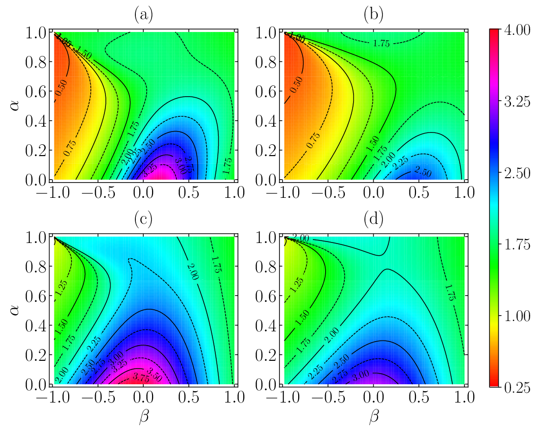
Now we go back to the general case and illustrate the dependence of the five transport coefficients , , , , and on the coefficients of restitution (, ) and the reduced moment of inertia () for both HS and HD granular gases. The results are displayed as density plots in Figs. 3–7. Two characteristic cases of mass distribution are considered: uniform distribution ( and for HD and HS, respectively) and mass concentrated on the outer surface ( and for HD and HS, respectively).
We observe an intricate influence of both and on the transport coefficients, with typically a strong nonmonotonic dependence on with, at fixed , a single maximum around for , , and , a maximum near for , and a more complex behavior for . Note that the bulk viscosity reaches very high values in the quasielastic and quasismooth region (see Fig. 4); in fact, as shown in Fig. 1 and Table 2, diverges in the combined limit and . Moreover, and are the transport coefficients more sensitive to the dimensionality and to the mass distribution. It is also worth mentioning that reaches negative values in a narrow lobe region near (see Fig. 7). That region is wider for HD than for HS and tends to shrink as the moment of inertia grows; in fact, it disappears for HS with a surface mass distribution.
VI Concluding remarks
In this study, we have considered a model of a granular gas as composed by spherical particles with constant coefficients of normal () and tangential () restitution. Previous results Kremer et al. 2014 for the transport coefficients of a dilute gas of inelastic and rough HS have been complemented with novel results for the parallel case of HD. We have developed this analysis in a unified vector space framework, based on previous works Megías and Santos 2019b; Megías and Santos 2019a, which allows us to obtain general expressions in terms of the number of translational () and rotational () degrees of freedom. The choice of the embedding Euclidean three-dimensional space is essential to get results for both geometries within a common framework. Particular aspects, especially the orthogonality condition between rotational and translational velocities in the HD case, permit us to neglect the computation of certain quantities and reduce them to already known HS terms being parameterized by or prefactors, as convenience, in the spirit of Refs. Megías and Santos 2019b; Megías and Santos 2019a.
The analysis has been carried out in the context of the nonlinear Boltzmann equation, where the system is assumed to be fully described by the one-particle VDF . Under the assumptions of (i) small gradients of the hydrodynamic fields [number density , flow velocity , and granular temperature ] and (ii) a “normal” solution (i.e., the space and time dependence of the one-particle VDF takes place through a functional dependence on , , and ), the Chapman–Enskog method has been used to solve the Boltzmann equation up to first order in the gradients. In that way, the NSF hydrodynamic equations are obtained by supplementing the balance equations for mass [Eq. (8a)], momentum [Eq. (8b)], and energy [Eq. (8e)] with constitutive equations for the pressure tensor [Eq. (34a)], the heat flux [Eq. (34b)], and the cooling rate [Eq. (32)].
The derivation of the associated transport coefficients has been carried out along three successive stages of increasing concreteness and level of approximation. In a first stage, the transport coefficients are expressed [see Eqs. (36) and (38)] in terms of collision integrals involving the zeroth-order (HCS) VDF and the functions , , , and characterizing the first-order VDF [see Eq. (29)]; those functions are the solutions of a set of linear integral equations [see Eqs. (30)] with inhomogeneous terms related to [see Eqs. (31)]. Next, in a second stage, Sonine-like forms for the functions , , , and are assumed [see Eqs. (40)], with coefficients (, , , , , and ) that can be expressed in terms of collisional integrals involving [see Eqs. (51) and (52)]. Finally, as the third and final stage, the HCS VDF is approximated by the product of a Maxwellian translational VDF times the marginal rotational VDF [see Eq. (14)]. The resulting explicit expressions for the transport coefficients as functions of the coefficients of restitution ( and ), the reduced moment of inertia (), and the numbers of degrees of freedom ( and ) are displayed in Table 1. In general, the transport coefficients exhibit a rather complex nonlinear dependence on , , and , as exposed in the density plots of Figs. 3–7.
The choice allows us to recover known results for three-dimensional HS Kremer et al. 2014, except that in our approach we did not need to assume a Maxwellian form for the marginal rotational VDF. Moreover, novel results for two-dimensional HD are derived via the choice . Thus, the outcome quantities can be used as a unified set of formulas for theoretical and experimental researchers, as well as a source of comparison between HD and HS setups.
Some special limiting cases have been exposed in Table 2: smooth, quasismooth, and Pidduck’s limits. The common description in terms of translational and rotational degrees of freedom let a direct recovery of the purely smooth case results by formally taking the limit at fixed , thus circumventing the singular nature of the quasismooth limit . In the latter limit, a universal lack of dependence on of the transport coefficients, already seen for HS Kremer et al. 2014, is observed. The quasismooth limit is quite distinct from the purely smooth case, as shown in Fig. 1. Furthermore, we have extended the original Pidduck’s system Pidduck 1922 () to our description, and novel results for HD are obtained; the dependencies with the reduced moment of inertia are shown in Fig. 2, where one can observe that the values of the coefficients and with a uniform mass distribution are similar for the two considered setups. It is also interesting to remark that the transport coefficient () associated with the velocity-divergence correction of the cooling rate vanishes in all these limits, for both HD and HS, as expected.
An immediate application of this work is the use of the closed set of NSF hydrodynamic equations to analyze the stability of the HCS, again in a unified framework encompassing the special HS and HD cases. This is the subject of the companion paper Megías and Santos 2021b. Additionally, the extension of the results to stochastically driven granular gases is straightforward (since the evaluation of the collision integrals has already been done in the present paper) and will be published elsewhere. Another future goal of our research is to go back to the second stage mentioned above and assume a form for where excess velocity kurtoses and translational-rotational velocity correlations are not neglected. Preliminary results Megías and Santos 2021a are quite promising.
Lastly, we hope that this research will inspire future works in the field, which could provide simulation and experimental results to compare with, as well as the introduction of alternative collisional models to describe systems of inelastic and rough particles.
Acknowledgements.
The authors acknowledge financial support from the Grant No. PID2020-112936GB-I00/AEI/10.13039/501100011033 and from the Junta de Extremadura (Spain) through Grants No. IB20079 and No. GR18079, all of them partially financed by Fondo Europeo de Desarrollo Regional funds. A.M. is grateful to the Spanish Ministerio de Ciencia, Innovación y Universidades for support from a predoctoral fellowship Grant No. FPU2018-3503.Appendix A Collision rules
The direct binary collision rules read
| (43) |
where is the impulse that particle exerts on particle . Our collision model is based on the existence of two constant coefficients of restitution, normal () and tangential (), which are defined by the following relations:
| (44) |
Here,
| (45) |
is the relative velocity of the contact points at the moment of collision, being the center-of-mass relative velocity and being directly related to the center-of-mass angular velocity. Then, from the conservation of angular and linear momenta in each collision, the impulse can be expressed as Kremer et al. 2014
| (46) |
where
| (47) |
The loss of energy due to inelasticity and roughness is observed in the change of total kinetic energy, which is given by
| (48) |
where . One can observe that, except if and either or , the total kinetic energy is dissipated upon collisions. This expected fact is translated into a decay of the total granular temperature in Sec. II.2.
The previous equations apply to both HS and HD. In the HS case, the translational velocity and the angular velocity have and nontrivial components, respectively. However, in the HD case, and have and nontrivial components, respectively, what simplifies the collision rules Santos 2018. An important consequence of the distinction between spheres and disks is that the Jacobian of the transformation between pre- and postcollisional velocities turns out to depend on , namely
| (49) |
Appendix B The coefficients in terms of collision integrals
References
- Campbell (1990) C. S. Campbell, Annu. Rev. Fluid Mech. 22, 57 (1990).
- Pöschel and Luding (2001) T. Pöschel and S. Luding, eds., Granular Gases, Lecture Notes in Physics, Vol. 564 (Springer, Berlin, 2001).
- Goldhirsch (2003) I. Goldhirsch, Rapid granular flows, Annu. Rev. Fluid Mech. 35, 267 (2003).
- Brilliantov and Pöschel (2004) N. V. Brilliantov and T. Pöschel, Kinetic Theory of Granular Gases (Oxford University Press, Oxford, 2004).
- Garzó (2019) V. Garzó, Granular Gaseous Flows. A Kinetic Theory Approach to Granular Gaseous Flows (Springer Nature, Switzerland, 2019).
- Yu et al. (2020) P. Yu, M. Schröter, and M. Sperl, Velocity distribution of a homogeneously cooling granular gas, Phys. Rev. Lett. 124, 208007 (2020).
- Jenkins and Richman (1985) J. T. Jenkins and M. W. Richman, Kinetic theory for plane flows of a dense gas of identical, rough, inelastic, circular disks, Phys. Fluids 28, 3485 (1985).
- Foerster et al. (1994) S. F. Foerster, M. Y. Louge, H. Chang, and K. Allia, Measurements of the collision properties of small spheres, Phys. Fluids 6, 1108 (1994).
- Walton (1993) O. R. Walton, Numerical simulations of inelastic, frictional particleparticle interactions, in Particle Two-Phase Flow, edited by M. C. Roco (Butterworth, London, 1993) pp. 884–907.
- (10)
M. Louge, http://grainflowresearch.mae.cornell.
edu/impact/data/Impact%20Results.html. - Jenkins and Zhang (2002) J. T. Jenkins and C. Zhang, Kinetic theory for identical, frictional, nearly elastic spheres, Phys. Fluids 14, 1228 (2002).
- Goldhirsch et al. (2005a) I. Goldhirsch, S. H. Noskowicz, and O. Bar-Lev, Nearly smooth granular gases, Phys. Rev. Lett. 95, 068002 (2005a).
- Goldhirsch et al. (2005b) I. Goldhirsch, S. H. Noskowicz, and O. Bar-Lev, Hydrodynamics of nearly smooth granular gases, J. Phys. Chem. B 109, 21449 (2005b).
- Brilliantov et al. (2007) N. V. Brilliantov, T. Pöschel, W. T. Kranz, and A. Zippelius, Translations and rotations are correlated in granular gases, Phys. Rev. Lett. 98, 128001 (2007).
- Gayen and Alam (2008) B. Gayen and M. Alam, Orientational correlation and velocity distributions in uniform shear flow of a dilute granular gas, Phys. Rev. Lett. 100, 068002 (2008).
- Mitrano et al. (2013) P. P. Mitrano, S. R. Dahl, A. M. Hilger, C. J. Ewasko, and C. M. Hrenya, Dual role of friction in granular flows: attenuation versus enhancement of instabilities, J. Fluid Mech. 729, 484 (2013).
- McNamara (1993) S. McNamara, Hydrodynamic modes of a uniform granular medium, Phys. Fluids A 5, 3056 (1993).
- Goldshtein and Shapiro (1995) A. Goldshtein and M. Shapiro, Mechanics of collisional motion of granular materials. Part 1. General hydrodynamic equations, J. Fluid Mech. 282, 75 (1995).
- Grossman et al. (1997) E. L. Grossman, T. Zhou, and E. Ben-Naim, Towards granular hydrodynamics in two dimensions, Phys. Rev. E 55, 4200 (1997).
- Sela and Goldhirsch (1998) N. Sela and I. Goldhirsch, Hydrodynamic equations for rapid flows of smooth inelastic spheres, to Burnett order, J. Fluid Mech. 361, 41 (1998).
- Dufty (2000) J. W. Dufty, Statistical mechanics, kinetic theory, and hydrodynamics for rapid granular flow, J. Phys.: Condens. Matter 12, A47 (2000).
- Dufty (2001) J. W. Dufty, Kinetic theory and hydrodynamics for a low density granular gas, Adv. Complex Syst. 4, 397 (2001).
- Garzó and Dufty (2002) V. Garzó and J. W. Dufty, Hydrodynamics for a granular mixture at low density, Phys. Fluids 14, 1476 (2002).
- Brilliantov and Pöschel (2003) N. Brilliantov and T. Pöschel, Hydrodynamics and transport coefficients for dilute granular gases, Phys. Rev. E 67, 061304 (2003).
- Serero et al. (2006) D. Serero, I. Goldhirsch, S. H. Noskowicz, and M.-L. Tan, Hydrodynamics of granular gases and granular gas mixtures, J. Fluid Mech. 554, 237 (2006).
- Vega Reyes and Urbach (2009) F. Vega Reyes and J. S. Urbach, Steady base states for Navier-Stokes granular hydrodynamics with boundary heating and shear, J. Fluid Mech. 636, 279 (2009).
- Vega Reyes et al. (2010) F. Vega Reyes, A. Santos, and V. Garzó, Non-Newtonian granular hydrodynamics. What do the inelastic simple shear flow and the elastic Fourier flow have in common?, Phys. Rev. Lett. 104, 028001 (2010).
- Dufty and Brey (2011) J. W. Dufty and J. J. Brey, Choosing hydrodynamic fields, Math. Model. Nat. Phenom. 6, 19 (2011).
- Garzó and Santos (2011) V. Garzó and A. Santos, Hydrodynamics of inelastic Maxwell models, Math. Model. Nat. Phenom. 6, 37 (2011).
- Gradenigo et al. (2011a) G. Gradenigo, A. Sarracino, D. Villamaina, and A. Puglisi, Fluctuating hydrodynamics and correlation lengths in a driven granular fluid, J. Stat. Mech. , P08017 (2011a).
- Gradenigo et al. (2011b) G. Gradenigo, A. Sarracino, D. Villamaina, and A. Puglisi, Non-equilibrium length in granular fluids: From experiment to fluctuating hydrodynamics, EPL 96, 14004 (2011b).
- García de Soria et al. (2013) M. I. García de Soria, P. Maynar, and E. Trizac, Linear hydrodynamics for driven granular gases, Phys. Rev. E 87, 022201 (2013).
- Pidduck (1922) F. B. Pidduck, The kinetic theory of a special type of rigid molecule, Proc. R. Soc. Lond. A 101, 101 (1922).
- Kremer et al. (2014) G. M. Kremer, A. Santos, and V. Garzó, Transport coefficients of a granular gas of inelastic rough hard spheres, Phys. Rev. E 90, 022205 (2014).
- Garzó et al. (2018) V. Garzó, A. Santos, and G. M. Kremer, Impact of roughness on the instability of a free-cooling granular gas, Phys. Rev. E 97, 052901 (2018).
- Megías and Santos (2019a) A. Megías and A. Santos, Energy production rates of multicomponent granular gases of rough particles. a unified view of hard-disk and hard-sphere systems, AIP Conf. Proc. 2132, 080003 (2019a).
- Megías and Santos (2019b) A. Megías and A. Santos, Driven and undriven states of multicomponent granular gases of inelastic and rough hard disks or spheres, Granul. Matter 21, 49 (2019b).
- Brey and Cubero (2001) J. J. Brey and D. Cubero, Hydrodynamic transport coefficients of granular gases, in Granular Gases, Lectures Notes in Physics, Vol. 564, edited by T. Pöschel and S. Luding (Springer, Berlin, 2001) pp. 59–78.
- Clement and Rajchenbach (1991) E. Clement and J. Rajchenbach, Fluidization of a bidimensional powder, Europhys. Lett. 16, 133 (1991).
- Feitosa and Menon (2002) K. Feitosa and N. Menon, Breakdown of energy equipartition in a 2D binary vibrated granular gas, Phys. Rev. Lett. 88, 198301 (2002).
- Painter et al. (2003) B. Painter, M. Dutt, and R. P. Behringer, Energy dissipation and clustering for a cooling granular material on a substrate, Physica D 175, 43 (2003).
- Yanpei et al. (2011) C. Yanpei, P. Evesque, M. Hou, C. Lecoutre, F. Palencia, and Y. Garrabos, Long range boundary effect of 2D intermediate number density vibro-fluidized granular media in micro-gravity, J. Phys.: Conf. Ser. 327, 012033 (2011).
- Grasselli et al. (2015) Y. Grasselli, G. Bossis, and R. Morini, Translational and rotational temperatures of a 2D vibrated granular gas in microgravity, Eur. Phys. J. E 38, 8 (2015).
- Scholz and Pöschel (2017) C. Scholz and T. Pöschel, Velocity distribution of a homogeneously driven two-dimensional granular gas, Phys. Rev. Lett. 118, 198003 (2017).
- Grasselli et al. (2017) Y. Grasselli, G. Bossis, A. Meunier, and O. Volkova, Dynamics of a 2D vibrated model granular gas in microgravity, in Granular Materials, edited by M. Sakellariou (IntechOpen, Rijeka, Croatia, 2017) Chap. 4, pp. 71–96.
- López-Castaño et al. (2021) M. A. López-Castaño, J. F. González-Saavedra, A. Rodríguez-Rivas, E. Abad, S. B. Yuste, and F. Vega Reyes, Pseudo-two-dimensional dynamics in a system of macroscopic rolling spheres, Phys. Rev. E 103, 042903 (2021).
- López Castaño et al. (2021) M. A. López Castaño, A. Márquez Seco, A. Márquez Seco, A. Rodríguez-Rivas, and F. Vega Reyes, Chirality transitions in a system of active flat spinners, arXiv:2105.02850 (2021).
- Garzó et al. (2007) V. Garzó, A. Santos, and J. M. Montanero, Modified Sonine approximation for the Navier–Stokes transport coefficients of a granular gas, Physica A 376, 94 (2007).
- Santos et al. (2011) A. Santos, G. M. Kremer, and M. dos Santos, Sonine approximation for collisional moments of granular gases of inelastic rough spheres, Phys. Fluids 23, 030604 (2011).
- Vega Reyes et al. (2014a) F. Vega Reyes, A. Santos, and G. M. Kremer, Role of roughness on the hydrodynamic homogeneous base state of inelastic spheres, Phys. Rev. E 89, 020202(R) (2014a).
- Vega Reyes et al. (2014b) F. Vega Reyes, A. Santos, and G. M. Kremer, Properties of the homogeneous cooling state of a gas of inelastic rough particles, AIP Conf. Proc. 1628, 494 (2014b).
- Garzó et al. (2012) V. Garzó, S. Tenneti, S. Subramaniam, and C. M. Hrenya, J. Fluid Mech. 712, 129 (2012).
- Chapman and Cowling (1970) S. Chapman and T. G. Cowling, The Mathematical Theory of Non-Uniform Gases, 3rd ed. (Cambridge University Press, Cambridge, UK, 1970).
- Kremer (2010) G. M. Kremer, An Introduction to the Boltzmann Equation and Transport Processes in Gases (Springer, Berlin, 2010).
- Megías and Santos (2021a) A. Megías and A. Santos, Translational and angular velocity cumulants in granular gases of inelastic and rough hard disks or spheres (unpublished) .
- Santos (2011) A. Santos, Homogeneous free cooling state in binary granular fluids of inelastic rough hard spheres, AIP Conf. Proc. 1333, 128 (2011).
- Santos et al. (2010) A. Santos, G. M. Kremer, and V. Garzó, Energy production rates in fluid mixtures of inelastic rough hard spheres, Prog. Theor. Phys. Suppl. 184, 31 (2010).
- McCoy et al. (1966) B. J. McCoy, S. I. Sandler, and J. S. Dahler, Transport properties of polyatomic fluids. IV. The kinetic theory of a dense gas of perfectly rough spheres, J. Chem. Phys. 45, 3485 (1966).
- Kudrolli (2010) A. Kudrolli, Concentration dependent diffusion of self-propelled rods, Phys. Rev. Lett. 104, 088001 (2010).
- Hall (2015) B. C. Hall, Lie Groups, Lie Algebras, and Representations. An Elementary Introduction, 2nd ed., Graduate Texts in Mathematics, Vol. 222 (Springer, Heidelberg, 2015).
- Guillard and Marks (2021) F. Guillard and B. Marks, Frictional hyperspheres in hyperspace, Phys. Rev. E 103, 052901 (2021).
- Megías and Santos (2021b) A. Megías and A. Santos, Hydrodynamics of granular gases of inelastic and rough hard disks or spheres. II. Stability analysis, Phys. Rev. E 104, 034902 (2021).
- Santos (2018) A. Santos, Interplay between polydispersity, inelasticity, and roughness in the freely cooling regime of hard-disk granular gases, Phys. Rev. E 98, 012904 (2018).