A generalized approach to compensate for low and high frequency errors in FFT based phase screen simulations
Abstract
Fast Fourier Transform based phase screen simulations give accurate results only when the screen size () is much larger than the outer scale parameter (). Otherwise, they fall short in correctly predicting both the low and high frequency behaviours of turbulence induced phase distortions. Sub-harmonic compensation is a commonly used technique that aids in low-frequency correction but does not solve the problem for all values of screen size to outer scale parameter ratios ). A subharmonics based approach will lead to unequal sampling or weights calculation for subharmonics addition at the low-frequency range and patch normalization factor. We have modified the subharmonics based approach by introducing a Gaussian phase autocorrelation matrix that compensates for these shortfalls. We show that the maximum relative error in structure function with respect to theoretical value is as small as 0.5-3% for ) ratio of 1/1000 even for screen sizes up to 100 m diameter.
keywords
Phase Screen, Fast Fourier Transform, Subharmonic, Autocorrelation, Phase structure function*Sorabh Chhabra, \linkablesorabh@iucaa.in / \linkablesorabh.chhabra@gmail.com
1 Introduction
Accurately simulating the atmospheric turbulence behaviour is well recognized as very challenging. For a variety of purposes such as the design and development of adaptive optics systems, speckle imaging techniques, atmospheric propagation studies etc., it is essential to simulate good atmospheric phase screen models. Methods based on Zernike polynomial expansions[1], FFT-based methods [2, 3, 4, 5, 6, 7, 8], Low Frequency Optimization method [9] etc. have been in use for this purpose. The Zernike polynomial method, which is widely in use, has a limitation due to the maximum number of coefficients needed for accurate compensation. The optimization method which compensates accurately for low frequency part of the spectrum by using unequal sampling and unequal weight in low frequency region, does not cover high frequency deficiencies. Among these, FFT-based methods are computer memory size friendly and widely accepted. But, FFT operators assume uniform sampling for the non-uniformly distributed phase power spectrum which can lead to underestimation in the low and high frequency out of band regions, as illustrated in Fig. 1. Thus, it has limitations in recreating the true phase power spectrum. To compensate for low-frequency components, Johansson and Gavel [3] suggested employing the modified subharmonics equation (an adaptation from Lane et al. [10]), which works well up to an infinite outer scale length. Sedmak [6] later compared the performance of this method with that of Lane et al. [10] by actually calculating the phase structure function from the simulated screen. He improved upon Lane et al. [10] by employing different fine tuned subharmonic weights for different ratios. Results from his analysis show that these FFT-based simulations are accurate for large screen size () to outer scale parameter () ratios. For a screen size of = 200 m and outer scale of = 25 m, the maximum relative error in the simulation approaches 1%. Our simulations demonstrate that the errors from low-frequency components start shooting up once we move to smaller ratios, even after compensating with modified subharmonics.
In Fig. 1 we illustrate [11] a typical situation where the simulation band is actually smaller than full band , where is the sampling size defined as the ratio of screen size to sampling number and is the inner scale parameter. In practice, the simulations are often curtailed at the low frequency end, to a few times the optical beam size (say as determined by the telescope or laser beam diameter), while at the high frequency end, they often extend to only a few times that determined by the Fried parameter . Clearly, the larger the simulation band to full band ratio, the more accurate the simulated results will be.
On the one hand, the apertures of upcoming and future astronomical telescopes are often of the same order or even larger than the typical median outer scale sizes of about 20 m - 25 m[12]. On the other hand, wavefront sensing and compensation technologies are fast progressing that Nyquist sampling at scales even for large aperture telescopes are becoming quite possible. Thus atmospheric turbulence simulations have to deal with a wide range in a multi-dimensional parameter space.

For working with very small apertures relative to the outer scale, it may appear that we need to simulate only a relatively small screen size. But cutting out small apertures from a larger screen introduces deviation from phase structure function due to misrepresentation of low frequency components present in the small screen power spectrum.
In this paper, we present an approach and a corresponding algorithm to deal with phase screen simulations for a wide range of ratios, using the FFT-based method. Our technique builds upon the modified subharmonic approach of Johansson and Gavel [3] and is inspired by Jingsong Xiang’s [13]. It works well for space- and time-invariant, zero intermittency atmospheric turbulence. Section 2 explains how to obtain phase autocorrealtion matrix using phase power spectrum, Section 3 presents the algorithm part to compensate for the remaining error in phase structure function calculation, Section 4 steps through the implementation of the algorithm with the help of a flow chart, Section 5 covers the validation of the technique using results from simulated phase screens, and Section 6 provides the concluding remarks.
2 Obtaining phase autocorrelation matrix using phase power spectrum
The 2D phase structure function and phase autocorrelation matrix are related as follows[14] :
| (1) |
where is the phase autocorrelation matrix and are the coordinates along x and y-axis. The 2D phase autocorrelation matrices for the FFT-based phase screen and the modified subharmonic method by Johansson and Gavel [3] are represented as follows.
| (2) |
| (3) |
where and are the von-Kármán spectrum and subharmonic power spectrum as explained by Johansson and Gavel. are sample points, p is the subharmonic and is the total number of subharmonics. Set = 0, for and = 0, for and as originally proposed by Lane et. al[10]. There will be an overlap between subharmonic energy sample and secondary lobes from first sample of high frequency spectrum or harmonic sample during subharmonic addition. Earlier this leakage of energy has been dealt using patch normalization factor, where first patch of high frequency spectrum is weighted by 0.707 for and and 0.866 for in the original method of Johansson and Gavel[3]. Similarly, the original method of Lane et al.[10], Sedmak[6] proposed the corresponding weights to be 0.935 and 0.998 respectively. Our simulations show that these weights do not fit perfectly for different ratios and hence need to be tuned on a case by case basis. We have made our approach independent from these weights assignments. The weight factor has been set equal to 1 in our approach. Section 3 explains this approach in detail.
The 2D phase autocorrelation matrix after compensating with subharmonics is represented as
| (4) |
3 Algorithm to compensate for residual error in phase structure function
To calculate the remaining error in the final , eq. (4) is converted to phase structure matrix with the help of eq. (1) with the assumption that and are zero because we are not concerned about the piston component. This gives the following equation
| (5) |
where is the well-known theoretical von-Kármán phase structure matrix [3], given as follows:
| (6) |
where , .
We need to compensate so that is minimized. However, simply adding error correction terms in the matrix directly would only introduce further error into the system, while taking the Fourier transform. This is because any matrix or curve in general will have higher order moments. Thus, if we take the Fourier transform of the adjusted equation, the resultant curve will have completely different moments and hence power spectrum. This is because the transition between two steps in the error matrix will not be smooth, which introduces additional errors due to Gibb’s phenomena like overshoots. Just curve fitting with any function does not satisfy the additional requirement of leaving the power spectrum unaffected by the process. What we really need is to introduce a smoothening operator like a Gaussian function in the phase autocorrelation matrix which exactly compensates for .
For that we have developed an iterative algorithm (see the flow chart shown in Fig. 4) and implemented it in Matlab. The algorithm looks for the perfect Gaussian curve that minimizes the matrix. We use Matlab cftool to initially determine the correct 1D Gaussian matrix and later convert it into a 2D matrix by exploiting the fact that (r), (r) and (r) all are dependent on r only and hence are centre symmetric functions. We call the fitted Gaussian phase structure matrix and the corresponding Gaussian phase autocorrelaiton matrix (using eq. (1)).
The final equation for can then be written as
| (7) |
Here we have used from eq. (1). A look at the power spectrum of in Fig 2 shows that it contains negative terms [7] for the case of . Directly putting those frequency terms equal to zero leads to a loss in the energy spectrum. Hence (m,n) matrix needs to be preprocessed to eliminate most of these negative values in the power spectrum. Over small frequencies, piston and tip/tilt components account for most of these high magnitude negative elements. Therefore, we first extract the piston and tip/tilt components from the phase autocorrelation matrix . The tip/tilt component from phase autocorrelation matrix is given as[7]


| (8) |
where is the variance of the random tilt angle in the x or y directions and given as follows[7]:
| (9) |
After setting, = 0, the remaining phase autocorrelation matrix is given as follows:
| (10) |
The power spectra and of the phase autocorrelation matrices and are obtained by standard fourier transformation. Fig. 3, shows the remaining negative power elements present in the power spectrum of matrix. In comparison to Fig. 2, the largest negative power contributions fall by factor of three order of magnitude. Now we set the negative values in equal to zero by hand. The new error matrix is given as:
| (11) |
where is the phase autocorrelation matrix obtained after setting the negative elements in to zero. The residual error that is present in the high frequency region can then be reduced with the help of a Gaussian smoothing operator, using Matlab fmincon tool. The high frequency compensated matrix is given as :
| (12) |
where is the smoothening operator, multiplied with error matrix to reduce the high frequency errors. fmincon gives the optimised parameter for smoothening operator by calculating the final error in the matrix w.r.t. .
4 Implementation of the compensation algorithm
In this section, we explain the error compensation algorithm with the help of the flow chart shown in Fig. 4. Brief explanations of each of the steps from to are given below.

- :
Input screen size , outer scale size , Fried parameter , and number of samples .
- :
Initialize the algorithm with , the total number of subharmonics and extrapolation factor EF, both ranging from 1 to 10. The EF factor is relevant while performing curve fitting. e.g. EF = 2 means curve fitting will work from 3 to N/2 points and later that curve will be extrapolated from 1 to N/2 points ( example shown in section 4.1, Fig. 6 )
- :
Obtain and based upon and parameters.
- :
Add the matrices that were calculated in layer, call that .
- :
- :
Obtain 1D array from matrix from the centre and give as input to the curve fitting tool cftool which works on 1D data. The output of the tool will be a best fitted curve in terms of Sum of Gaussian’s (SoG), called
- :
The final expression for is shown eq. (7).
- :
fmincon: High Frequency error Optimization
- :
Obtain error matrix after setting negative elements in the power spectrum to zero. Compensate for high frequency error by multiplying error matrix with smoothening operator-SoG. Calculate the maximum remaining error in structure function matrix relative to the matrix. Thus fmincon will give parameters for the smoothing operator, that gives the lowest possible residual error.
- :
Update the entry for EF to next value, evaluation from - would go in loop, and MRE value stored in vector form. At the end of the iterations, min entry will get extracted out from stored vector and accepted for final analysis.
Table 1 shows the result of curve fitting using cftool for different cases of and N, which demonstrates that the Gaussian error matrix can compensate for a wide range of ratios and under different sampling constraints.
| = 128 | = 256 | = 512 | = 1024 | ||||||||||||||
| SoG | MRE(%) | SoG | MRE(%) | SoG | MRE(%) | SoG | MRE(%) | ||||||||||
| 1 | 20 | 2 | 1 | 3 | 0.25 | 2 | 2 | 4 | 0.61 | 2 | 2 | 3 | 0.36 | 2 | 1 | 4 | 1 |
| 5 | 20 | 1 | 1 | 5 | 0.19 | 6 | 3 | 5 | 0.23 | 4 | 2 | 3 | 0.27 | 7 | 1 | 3 | 1 |
| 10 | 20 | 9 | 5 | 4 | 0.25 | 9 | 1 | 5 | 0.29 | 1 | 1 | 3 | 0.26 | 7 | 3 | 6 | 0.35 |
| 20 | 20 | 3 | 1 | 4 | 0.53 | 10 | 1 | 6 | 0.4 | 4 | 5 | 5 | 0.97 | 3 | 5 | 3 | 0.22 |
| 40 | 20 | 5 | 0 | 4 | 0.95 | 8 | 0 | 6 | 0.75 | 8 | 0 | 3 | 1 | 7 | 1 | 3 | 2.99 |
| 60 | 20 | 5 | 0 | 4 | 0.17 | 3 | 2 | 6 | 0.42 | 9 | 8 | 5 | 0.41 | 3 | 1 | 5 | 0.94 |
| 80 | 20 | 8 | 1 | 4 | 0.24 | 7 | 5 | 3 | 0.17 | 5 | 6 | 3 | 0.32 | 6 | 4 | 3 | 0.3 |
| 100 | 20 | 8 | 1 | 4 | 0.24 | 7 | 5 | 3 | 0.17 | 5 | 6 | 3 | 0.32 | 6 | 4 | 3 | 0.3 |
| 1 | 10 | 3 | 1 | 4 | 0.53 | 10 | 1 | 6 | 0.4 | 4 | 5 | 5 | 0.97 | 3 | 5 | 3 | 0.22 |
| 1 | 100 | 3 | 1 | 6 | 0.21 | 4 | 1 | 4 | 0.49 | 3 | 6 | 5 | 0.96 | 3 | 6 | 5 | 0.25 |
| 1 | 1000 | 5 | 0 | 4 | 0.95 | 8 | 0 | 6 | 0.75 | 8 | 0 | 3 | 1 | 7 | 1 | 3 | 2.99 |
| 10 | 100 | 2 | 0 | 6 | 0.28 | 3 | 0 | 4 | 0.22 | 8 | 1 | 4 | 0.30 | 7 | 0 | 3 | 0.27 |
| 10 | 1000 | 5 | 0 | 4 | 0.17 | 3 | 2 | 6 | 0.42 | 9 | 8 | 5 | 0.41 | 3 | 1 | 5 | 0.94 |
| 100 | 100 | 3 | 0 | 6 | 0.21 | 2 | 3 | 5 | 0.21 | 7 | 0 | 3 | 0.26 | 1 | 1 | 3 | 0.26 |
| 100 | 1000 | 8 | 1 | 4 | 0.24 | 7 | 5 | 3 | 0.17 | 5 | 6 | 3 | 0.32 | 6 | 4 | 3 | 0.3 |
4.1 Example
To illustrate the robustness of the above algorithm, we have taken an example with G = 80 m, say for a large future telescope, N = 256, and median value of = 20 m.
The output from the above algorithm corresponding to minimum error entry as in (step ), has been plotted against = 5 and = 8. Fig. 5 gives a 3D rendering of matrix with a maximum separation of up to 40 m, corresponding to eq. (4).

Fig. 6 represents 1D matrix ( radial section from 3D matrix ) along with 1D fitted curve including the extrapolated part, for a maximum separation of up to 40 m.

Lastly, MRE values are stored against 500 entries corresponding to ranging from 1 to 10, ranging from 1 to 10 and ranging from 2 to 6 after performing cftool fitting. This has been arranged in descending order and presented in Fig. 7, which illustrates a large set of iterations where errors are less than 1% and entry with minimum MRE has been picked up. Typical time required to perform each iteration for this case is 4.9 sec on 2.3GHz quad-core Intel Core i5 Macbook pro 2018 model.

5 Validation via phase structure function calculated from simulated phase screen
To obtain the phase screen from the power spectrum, the following relation is used[7]:
| (13) |
where and are zero-mean and unity-variance gaussian random number generator. We get and , by replacing with and , which are square roots of the power spectrum corresponding to autocorrelation matrix and respectively.
For validation, we consider scenarios of apertures up to 40 m i.e = 80 m, at a median = 20 m for two different sampling levels N = 256 and 512. The phase structure function, defined as an ensemble average of differences of phases at various separation[14], has been averaged over 100K independent frames. The relative error in phase structure function is calculated as follows:
| (14) |
Here, is the phase structure function from the simulated phase screen. The magnitude of the peak relative error is for = 256 and for = 512 as shown in Fig. 8.
We also illustrate the performance ( shown in Fig. 9 ) with parameters G = 1 m, = 100 m and 1000 m, N = 128, = 0.2 m which cover the extreme cases ( very low ratios ) which leads to the maximum error in the simulation. The magnitude of the peak relative error is for = 100 m and for = 1000 m. Fig. 10 shows one realization of the corresponding phase screen plots for = 100 m.

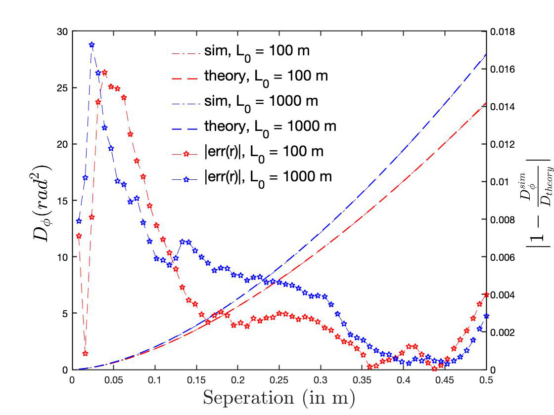
Fig. 11 contains results of magnitude of the peak relative error in for the case of different sampling points = 128/256/512/1024, for ranges up to 1024 m, = 0.2 m and = 2 m. Similarly, Fig. 12 contains results of magnitude of the peak relative error in for the case of different sampling points = 128/256/512/1024, for ranges up to 100 m, = 0.2 m and = 25 m.


There are some outliers which have a high residual error as shown in Fig. 11 and Fig. 12, because we have not set the phase autocorrelation matrix to zero for . The reason for this stems from the non-zero value of at , where is formed from the removal of piston and tilt from . This can be resolved by using a better smoothening operator, which we can multiply with so that it falls to zero progressively and not sharply. This can provide further improvement in the compensation.
6 Conclusion
In this paper, we put forward a new method to compensate for the residual error in both the Low and/or High-frequency region of FFT simulated phase screens that remain even after compensating with the modified subharmonic method. This method provides accurate phase screen structure for even ratios as small as 1/1000 plus screen sizes as large as 100 m. No Patch Normalization factor is needed, no need to calculate subharmonic weight coefficient [10] and weights to compensate for high-frequency components, as done by Sedmak[6]. While adequately large ratios may be the natural choice for modern large telescopes, simulations that deal with applications such as laser beam propagation through turbulent atmospheres would tend to have very small ratios. The method we propose is independent of the ratio choice. However, we emphasize that properly sampling and the high-frequency phase spectrum forces to be at least larger than and preferably up to the inner scale limit . Currently we have demonstrated this technique for only circular screens. We have used a GPU processor with total number of 128 cores, such that each iteration runs independently on each core. We have fixed the number of iterations to 500, although increasing this will lead to improvement of errors in some cases. Each core takes about 0.06, 0.1, 0.36 and 1.1 minutes for sampling sizes of 128, 256, 512 and 1024. On the above GPU system, this translates to total computing times for error minimization of about 0.2, 0.5, 1.25 and 4 minutes for sampling sizes of 128, 256, 512 and 1024 respectively. Once the coefficients are determined, generating multiple phase screen realizations from the corresponding power spectrum takes a few milliseconds at most on 2.3 GHz quad-core Intel Core i5 Macbook pro 2018 model. Then it takes less than a minute to 10 min for averaging over 100k phase screens, for sampling sizes ranging from 128 to 1024.
The uniqueness of our approach is its ability to deal with any ratio within a very broad range, in an automated iterative process with little human intervention needed for tuning of parameters. Any standard FFT based approach (say Sedmak’s[6] compensated approach) for a given computer platform is computationally fast, only if we already have determined proper measures of the various compensating components such as the patch normalization factor, subharmonic weights, high-frequency weights etc. Typically, determining these compensations is where the difficulty is due to mathematical complexity, algorithmic limitations and/or computational power requirements. Our algorithm accomplishes the determination of the required compensation in very little time, with fairly reasonable computational power while at the same time keeping the residual errors competitively low by using an appropriate compensator. Other existing FFT based approaches have limitations in their operable range. For example, Xiang et. al.[7] offer a very computationally fast approach but does not apply subharmonic compensation. Zhang et. al.[9] does not consider compensation for the high-frequency error, thus leaving a residual error of more than 100% in the high-frequency region. Sedmak’s[6] approach needs the determination of accurate subharmonic weights for different ratios. The accuracy of our method from low-frequency to the high-frequency range is between 0.5-3% for as low as 1/1000 and screen size up to 100 m in diameter.
Acknowledgements.
We would like to thank Sedmak for providing insights into the nature of atmospheric phase power spectrum through private communication. We also thank Xiang for sharing his MATLAB code which calculates the phase structure function quickly for a large number of phase screens. We acknowledge usage of IUCAA’s Pegasus cluster computer for running multiple independent iterations in parallel.References
- [1] N. A. Roddier, “Atmospheric wavefront simulation and zernike polynomials,” in Amplitude and Intensity Spatial Interferometry, 1237, 668–679, International Society for Optics and Photonics (1990).
- [2] B. J. Herman and L. A. Strugala, “Method for inclusion of low-frequency contributions in numerical representation of atmospheric turbulence,” in Propagation of High-Energy Laser Beams through the Earth’s Atmosphere, 1221, 183–192, International Society for Optics and Photonics (1990).
- [3] E. M. Johansson and D. T. Gavel, “Simulation of stellar speckle imaging,” in Amplitude and Intensity Spatial Interferometry II, 2200, 372–383, International Society for Optics and Photonics (1994).
- [4] G. Sedmak, “Performance analysis of and compensation for aspect-ratio effects of fast-fourier-transform-based simulations of large atmospheric wave fronts,” Applied optics 37(21), 4605–4613 (1998).
- [5] B. L. McGlamery, “Computer simulation studies of compensation of turbulence degraded images,” in Image processing, 74, 225–233, International Society for Optics and Photonics (1976).
- [6] G. Sedmak, “Implementation of fast-fourier-transform-based simulations of extra-large atmospheric phase and scintillation screens,” Applied optics 43(23), 4527–4538 (2004).
- [7] J. Xiang, “Fast and accurate simulation of the turbulent phase screen using fast fourier transform,” Optical Engineering 53(1), 016110 (2014).
- [8] J. Xiang, “Accurate compensation of the low-frequency components for the fft-based turbulent phase screen,” Optics express 20(1), 681–687 (2012).
- [9] D. Zhang, Z. Chen, C. Xiao, et al., “Accurate simulation of turbulent phase screen using optimization method,” Optik 178, 1023–1028 (2019).
- [10] R. Lane, A. Glindemann, J. Dainty, et al., “Simulation of a kolmogorov phase screen,” Waves in random media 2(3), 209–224 (1992).
- [11] G. Sedmak. private communication (2019).
- [12] A. Ziad, “Review of the outer scale of the atmospheric turbulence,” in Adaptive Optics Systems V, 9909, 99091K, International Society for Optics and Photonics (2016).
- [13] S. Chhabra, J. Paul, A. Ramaprakash, et al., “Gaussian phase autocorrelation as an accurate compensator for fft-based atmospheric phase screen simulations,” in Adaptive Optics Systems VII, 11448, 114487U, International Society for Optics and Photonics (2020).
- [14] F. Roddier, Adaptive optics in astronomy, Cambridge university press (1999).
Sorabh Chhabra is a PhD student at Inter University Center for Astronomy and Astrophysics (IUCAA), Pune. He received his B.Tech degree in Electronics and Communication from Delhi Technological University (formally Delhi College of Engineering ) in 2016 and joined for his PhD in the same year in Instrumentation department at IUCAA.
List of Figures
List of Tables