跳到论文正文
W Papers独立论文阅读器 arXiv:2106.00885 论文正文 计算阅读时间 · 0%
引用这篇论文根据当前论文元数据生成,正式投稿前建议核对。


License: arXiv.org perpetual non-exclusive license
arXiv:2106.00885v3 [stat.ML] 25 Oct 2021

Robustifying Algorithms of Learning Latent Trees with Vector Variables

Fengzhuo Zhang Affiliation: Department of Electrical and Computer Engineering Affiliation: National University of Singapore Email: fzzhang@u.nus.edu    Vincent Y. F. Tan Affiliation: Department of Electrical and Computer Engineering Affiliation: Department of Mathematics Affiliation: National University of Singapore Email: vtan@nus.edu.sg
Abstract

We consider learning the structures of Gaussian latent tree models with vector observations when a subset of them are arbitrarily corrupted. First, we present the sample complexities of rg (rg) and clrg (clrg) without the assumption that the effective depth is bounded in the number of observed nodes, significantly generalizing the results in Choi et al. (2011). We show that Chow-Liu initialization in clrg greatly reduces the sample complexity of rg from being exponential in the diameter of the tree to only logarithmic in the diameter for the hmm (hmm). Second, we robustify rg, clrg, nj (nj) and snj (snj) by using the truncated inner product. These robustified algorithms can tolerate a number of corruptions up to the square root of the number of clean samples. Finally, we derive the first known instance-dependent impossibility result for structure learning of latent trees. The optimalities of the robust version of clrg and nj are verified by comparing their sample complexities and the impossibility result.

1 Introduction

Latent graphical models provide a succinct representation of the dependencies among observed and latent variables. Each node in the graphical model represents a random variable or a random vector, and the dependencies among these variables are captured by the edges among nodes. Graphical models are widely used in domains from biology [1], computer vision [2] and social networks [3].

This paper focuses on the structure learning problem of latent tree-structured ggm (ggm) in which the node observations are random vectors and a subset of the observations can be arbitrarily corrupted. This classical problem, in which the variables are clean scalar random variables, has been studied extensively in the past decades. The first information distance-based method, nj, was proposed in [1] to learn the structure of phylogenetic trees. This method makes use of additive information distances to deduce the existence of hidden nodes and introduce edges between hidden and observed nodes. rg, proposed in [4], generalizes the information distance-based methods to make it applicable for the latent graphical models with general structures. Different from these information distance-based methods, quartet-based methods [5] utilize the relative geometry of every four nodes to estimate the structure of the whole graph. Although experimental comparisons of these algorithms were conducted in some works [4, 6, 7], since there is no instance-dependent impossibility result of the sample complexity of structure learning problem of latent tree graphical models, no thorough theoretical comparisons have been made, and the optimal dependencies on the diameter of graphs and the maximal distance between nodes ρmax\rho_{\max} have not been found.

The success of the previously-mentioned algorithms relies on the assumption that the observations are i.i.d. samples from the generating distribution. The structure learning of latent graphical models in presence of (random or adversarial) noise remains a relatively unexplored problem. The presence of the noise in the samples violates the i.i.d. assumption. Consequently, classical algorithms may suffer from severe performance degradation in the noisy setting. There are some works studying the problem of structure learning of graphical models with noisy samples, where all the nodes in the graphical models are observed and not hidden. Several assumptions on the additive noise are made in these works, which limit the use of these proposed algorithms. For example, the covariance matrix of the noise is specified in [8], and the independence and/or distribution of the noise is assumed in [9, 10, 11, 7]. In contrast, we consider the structure learning of latent tree graphical models with arbitrary corruptions, where assumptions on the distribution and independence of the noise across nodes are not required [12]. Furthermore, the corruptions are allowed to be presented at any position in the data matrix; they do not appear solely as outliers. In this work, we derive bounds on the maximum number of corruptions that can be tolerated for a variety of algorithms, and yet structure learning can succeed with high probability.

Firstly, we derive the sample complexities of rg and clrg where each node represents a random vector; this differs from previous works where each node is scalar random variable (e.g., [4, 13]). We explore the dependence of the sample complexities on the parameters of the graph. Compared with [4, Theorem 12], the derived sample complexities are applicable to a wider class of latent trees and capture the dependencies on more parameters of the underlying graphical models, such as ρmax\rho_{\max}, the maximum distance between any two nodes, and δmin\delta_{\min}, the minimum over all determinants of the covariance matrices of the vector variables. Our sample complexity analysis clearly demonstrates and precisely quantifies the effectiveness of the Chow-Liu [14] initialization step in clrg; this has been only verified experimentally [4]. For the particular case of the hmm, we show that the Chow-Liu initialization step reduces the sample complexity of rg which is O⁡((92)Diam⁡(𝕋))O\big((\frac{9}{2})^{\mathrm{Diam}(\mathbb{T})}\big) to O⁡(log⁡Diam⁡(𝕋))O\big(\log\mathrm{Diam}(\mathbb{T})\big), where Diam⁡(𝕋)\mathrm{Diam}(\mathbb{T}) is the tree diameter.

Secondly, we robustify rg, clrg, nj and snj by using the truncated inner product [15] to estimate the information distances in the presence of arbitrary corruptions. We derive their sample complexities and show that they can tolerate n1=O⁡(n2log⁡n2)n_{1}=O\big(\frac{\sqrt{n_{2}}}{\log n_{2}}\big) corruptions, where n2n_{2} is the number of clean samples.

Finally, we derive the first known instance-dependent impossibility result for learning latent trees. The dependencies on the number of observed nodes |𝒱obs||\mathcal{V}_{\mathrm{obs}}| and the maximum distance ρmax\rho_{\max} are delineated. The comparison of the sample complexities of the structure learning algorithms and the impossibility result demonstrates the optimality of rclrg (rclrg) and rnj (rnj) in Diam⁡(𝕋)\mathrm{Diam}(\mathbb{T}) for some archetypal latent tree structures.

Notation

We use san-serif letters xx, boldface letters 𝐱\mathbf{x}, and bold uppercase letters 𝐗\mathbf{X} to denote variables, vectors and matrices, respectively. The notations [𝐱]i[\mathbf{x}]_{i}, [𝐗]i​j[\mathbf{X}]_{ij}, [𝐗]:,j[\mathbf{X}]_{:,j} and diag⁡(𝐗)\mathrm{diag}(\mathbf{X}) are respectively the ithi^{\mathrm{th}} entry of vector 𝐱\mathbf{x}, the (i,j)th(i,j)^{\mathrm{th}} entry of 𝐗\mathbf{X}, the jthj^{\mathrm{th}} column of 𝐗\mathbf{X}, and the diagonal entries of matrix 𝐗\mathbf{X}. The notation x(k)x^{(k)} represents the kthk^{\mathrm{th}} sample of xx. ‖𝐱‖0\|\mathbf{x}\|_{0} is the l0l_{0} norm of the vector 𝐱\mathbf{x}, i.e., the number of non-zero terms in 𝐱\mathbf{x}. The set {1,…,n}\{1,\ldots,n\} is denoted as [n][n]. For a tree 𝕋=(𝒱,ℰ)\mathbb{T}=(\mathcal{V},\mathcal{E}), the internal (non-leaf) nodes, the maximal degree and the diameter of 𝕋\mathbb{T} are denoted as Int⁡(𝕋)\mathrm{Int}(\mathbb{T}), Deg⁡(𝕋)\mathrm{Deg}(\mathbb{T}), and Diam⁡(𝕋)\mathrm{Diam}(\mathbb{T}), respectively. We denote the closed neighborhood and the degree of xix_{i} as nbd⁡[xi;𝕋]\mathrm{nbd}[x_{i};\mathbb{T}] and deg⁡(i)\mathrm{deg}(i), respectively. The length of the (unique) path connecting xix_{i} and xjx_{j} is denoted as d𝕋​(xi,xj)\mathrm{d}_{\mathbb{T}}(x_{i},x_{j}).

2 Preliminaries and problem statement

A ggm [16, 17] is a multivariate Gaussian distribution that factorizes according to an undirected graph 𝔾=(𝒱,ℰ)\mathbb{G}=(\mathcal{V},\mathcal{E}). More precisely, a lsuml_{\mathrm{sum}}-dimensional random vector 𝐱=[𝐱1⊤,…,𝐱p⊤]⊤\mathbf{x}=[\mathbf{x}_{1}^{\top},\ldots,\mathbf{x}_{p}^{\top}]^{\top}, where 𝐱i∈ℝli\mathbf{x}_{i}\in\mathbb{R}^{l_{i}} and lsum=∑i=1plil_{\mathrm{sum}}=\sum_{i=1}^{p}l_{i}, follows a Gaussian distribution 𝒩⁡(𝟎,𝚺)\mathcal{N}(\mathbf{0},\mathbf{\Sigma}), and it is said to be Markov on a graph 𝔾=(𝒱,ℰ)\mathbb{G}=(\mathcal{V},\mathcal{E}) with vertex set 𝒱={x1,…,xp}\mathcal{V}=\{x_{1},\ldots,x_{p}\} and edge set ℰ⊆(𝒱2)\mathcal{E}\subseteq\binom{\mathcal{V}}{2} and (xi,xj)∈ℰ(x_{i},x_{j})\in\mathcal{E} if and only if the (i,j)th(i,j)^{\mathrm{th}} block 𝚯i​j\mathbf{\Theta}_{ij} of the precision 𝚯=𝚺−1\mathbf{\Theta}=\mathbf{\Sigma}^{-1} is not the zero matrix 𝟎\mathbf{0}. We focus on tree-structured graphical models, which factorize according to acyclic and connected (tree) graphs.

A special class of graphical models is the set of latent graphical models 𝔾=(𝒱,ℰ)\mathbb{G}=(\mathcal{V},\mathcal{E}). The vertex set 𝒱\mathcal{V} is decomposed as 𝒱=𝒱hid∪𝒱obs\mathcal{V}=\mathcal{V}_{\mathrm{hid}}\cup\mathcal{V}_{\mathrm{obs}}. We only have access to nn i.i.d. samples drawn from the observed set of nodes 𝒱obs\mathcal{V}_{\mathrm{obs}}. The two goals of any structure learning algorithm are to learn the identities of the hidden nodes 𝒱hid\mathcal{V}_{\mathrm{hid}} and how they are connected to the observed nodes.

2.1 System model for arbitrary corruptions

We consider tree-structured ggms 𝕋=(𝒱,ℰ)\mathbb{T}=(\mathcal{V},\mathcal{E}) with observed nodes 𝒱obs={x1,⋯,xo}\mathcal{V}_{\mathrm{obs}}=\{x_{1},\cdots,x_{o}\} and hidden nodes 𝒱hid={xo+1,⋯,xo+h}\mathcal{V}_{\mathrm{hid}}=\{x_{o+1},\cdots,x_{o+h}\}, where 𝒱=𝒱hid∪𝒱obs\mathcal{V}=\mathcal{V}_{\mathrm{hid}}\cup\mathcal{V}_{\mathrm{obs}} and ℰ⊆(𝒱2)\mathcal{E}\subseteq\binom{\mathcal{V}}{2}. Each node xix_{i} represents a random vector 𝐱i∈ℝli\mathbf{x}_{i}\in\mathbb{R}^{l_{i}}. The concatenation of these random vectors is a multivariate Gaussian random vector with zero mean and covariance matrix 𝚺\mathbf{\Sigma} with size lsum×lsuml_{\mathrm{sum}}\times l_{\mathrm{sum}}.

We have nn i.i.d. samples 𝐗~j=[𝐱~1(j)⊤,⋯,𝐱~o(j)⊤]⊤∈ℝlsum,j=1,…,n\tilde{\mathbf{X}}_{j}=[\tilde{\mathbf{x}}_{1}^{(j)\top},\cdots,\tilde{\mathbf{x}}_{o}^{(j)\top}]^{\top}\in\mathbb{R}^{l_{\mathrm{sum}}},j=1,\ldots,n drawn from the observed nodes 𝒱obs={x1,⋯,xo}\mathcal{V}_{\mathrm{obs}}=\{x_{1},\cdots,x_{o}\}. However, the observed data matrix 𝐗~1n=[𝐗~1,⋯,𝐗~n]⊤∈ℝn×lsum\tilde{\mathbf{X}}_{1}^{n}=[\tilde{\mathbf{X}}_{1},\cdots,\tilde{\mathbf{X}}_{n}]^{\top}\in\mathbb{R}^{n\times l_{\mathrm{sum}}} may contain some corrupted elements. We allow an level-(n1/2)(n_{1}/2) arbitrary corruption in the data matrix. This is made precise in the following definition.

Definition 1 (Level-mm arbitrary corruption).

For the data matrix 𝐗~1n∈ℝn×k\tilde{\mathbf{X}}_{1}^{n}\in\mathbb{R}^{n\times k} formed by nn clean samples of kk random variables (or a random vector of dimension kk), an level-mm arbitrary corruption transforms 𝐗~1n\tilde{\mathbf{X}}_{1}^{n} into 𝐗1n∈ℝn×k\mathbf{X}_{1}^{n}\in\mathbb{R}^{n\times k} such that

∥[𝐗~1n];,i−[𝐗1n];,i∥0≤m for all i=1,…,k.\displaystyle\|[\tilde{\mathbf{X}}_{1}^{n}]_{;,i}-[\mathbf{X}_{1}^{n}]_{;,i}\|_{0}\leq m\quad\text{ for all }\quad i=1,\ldots,k. (1)

Definition 1 implies that there are at most n1/2n_{1}/2 corrupted terms in each column of 𝐗1n\mathbf{X}_{1}^{n}; the remaining n−n1/2n-n_{1}/2 samples in this column are clean. In particular, the corrupted samples in different columns need not to be in the same rows. If the corruptions in different columns lie in the same rows, as shown in (the left of) Fig. 3, all the samples in the corresponding rows are corrupted; these are called outliers. Obviously, outliers form a special case of our corruption model. Since each variable has at most n1/2n_{1}/2 corrupted samples, the sample-wise inner product between two variables has at least n2=n−n1n_{2}=n-n_{1} clean samples. There is no constraint on the statistical dependence or patterns of the corruptions. Unlike fixing the covariance matrix of the noise [8] or keeping the noise independent [9], we allow arbitrary corruptions on the samples, which means that the noise can have unbounded amplitude, can be dependent, and even can be generated from another graphical model (as we will see in the experimental results in Section 3.6).

2.2 Structural and distributional assumptions

To construct the correct latent tree from samples of observed nodes, it is imperative to constrain the class of latent trees to guarantee that the information from the distribution of observed nodes p⁡(𝐱1,…,𝐱o)p(\mathbf{x}_{1},\ldots,\mathbf{x}_{o}) is sufficient to construct the tree. The distribution p⁡(𝐱1,…,𝐱o+h)p(\mathbf{x}_{1},\ldots,\mathbf{x}_{o+h}) of the observed and hidden nodes is said to have a redundant hidden node xjx_{j} if the distribution of the observed nodes p⁡(𝐱1,…,𝐱o)p(\mathbf{x}_{1},\ldots,\mathbf{x}_{o}) remains the same after we marginalize over xjx_{j}. To ensure that a latent tree can be constructed with no ambiguity, we need to guarantee that the true distribution does not have any redundant hidden node(s), which is achieved by following two conditions [18]: (C1) Each hidden node has at least three neighbors; the set of such latent trees is denoted as 𝒯≥3\mathcal{T}_{\geq 3}; (C2) Any two variables connected by an edge are neither perfectly dependent nor independent.

Assumption 1.

The dimensions of all the random vectors are all equal to lmaxl_{\max}.

In fact, we only require the random vectors of the internal (non-leaf) nodes to have the same length. However, for ease of notation, we assume that the dimensions of all the random vectors are lmaxl_{\max}.

Assumption 2.

For every xi,xj∈𝒱x_{i},x_{j}\in\mathcal{V}, the covariance matrix 𝚺i​j=𝔼⁡[𝐱i​𝐱j⊤]\mathbf{\Sigma}_{ij}=\mathbb{E}\big[\mathbf{x}_{i}\mathbf{x}_{j}^{\top}\big] has full rank, and the smallest singular value of 𝚺i​j\mathbf{\Sigma}_{ij} is lower bounded by γmin\gamma_{\min}, i.e.,

σlmax​(𝚺i​j)≥γminfor allxi,xj∈𝒱,\displaystyle\sigma_{l_{\max}}(\mathbf{\Sigma}_{ij})\geq\gamma_{\min}\quad\text{for all}\quad x_{i},x_{j}\in\mathcal{V}, (2)

where σi​(𝚺)\sigma_{i}(\mathbf{\Sigma}) is the ithi^{\mathrm{th}} largest singular value of 𝚺\mathbf{\Sigma}.

This assumption is a strengthening of Condition (C2) when each node represents a random vector.

Assumption 3.

The determinant of the covariance matrix of any node 𝚺i​i=𝔼⁡[𝐱i​𝐱i⊤]\mathbf{\Sigma}_{ii}=\mathbb{E}\big[\mathbf{x}_{i}\mathbf{x}_{i}^{\top}\big] is lower bounded by δmin\delta_{\min}, and the diagonal terms of the covariance matrix are upper bounded by σmax2\sigma_{\max}^{2}, i.e.,

min⁡detxi∈𝒱⁡(𝚺i​i)≥δminandmaxxi∈𝒱⁡diag⁡(𝚺i​i)≤σmax2.\displaystyle\min_{x_{i}\in\mathcal{V}}\det(\mathbf{\Sigma}_{ii})\geq\delta_{\min}\quad\mbox{and}\quad\max_{x_{i}\in\mathcal{V}}\mathrm{diag}\big(\mathbf{\Sigma}_{ii}\big)\leq\sigma_{\max}^{2}. (3)

Assumption 3 is natural; otherwise, 𝚺i​i\mathbf{\Sigma}_{ii} may be arbitrarily close to a singular matrix.

Assumption 4.

The degree of each node is upper bounded by dmaxd_{\max}, i.e., Deg⁡(𝕋)≤dmax\mathrm{Deg}(\mathbb{T})\leq d_{\max}.

2.3 Information distance

We define the information distance for Gaussian random vectors and prove that it is additive for trees.

Definition 2.

The information distance between nodes xix_{i} and xjx_{j} is

d⁡(xi,xj)=−log⁡∏k=1lmaxσk​(𝚺i​j)det⁡(𝚺i​i)​det​(𝚺j​j).\displaystyle\mathrm{d}(x_{i},x_{j})=-\log\frac{\prod_{k=1}^{l_{\max}}\sigma_{k}\big(\mathbf{\Sigma}_{ij}\big)}{\sqrt{\mathrm{det}\big(\mathbf{\Sigma}_{ii}\big)\mathrm{det}\big(\mathbf{\Sigma}_{jj}\big)}}. (4)

Condition (C2) can be equivalently restated as constraints on the information distance.

Assumption 5.

There exist two constants 0<ρmin≤ρmax<∞0<\rho_{\min}\leq\rho_{\max}<\infty such that.

ρmin≤d⁡(xi,xj)≤ρmaxfor allxi,xj∈𝒱.\displaystyle\rho_{\min}\leq\mathrm{d}(x_{i},x_{j})\leq\rho_{\max}\quad\text{for all}\quad x_{i},x_{j}\in\mathcal{V}. (5)

Assumptions 2 and 5 both describe the properties of the correlation between random vectors from different perspectives. In fact, we can relate the constraints in these two assumptions as follows:

γmin​eρmax/lmax≥δmin1/lmax.\displaystyle\gamma_{\min}e^{\rho_{\max}/l_{\max}}\geq\delta_{\min}^{1/l_{\max}}. (6)
Proposition 1.

If Assumptions 1 and 2 hold, d⁡(⋅,⋅)\mathrm{d}(\cdot,\cdot) defined in Definition 2 is additive on the tree-structured ggm 𝕋=(𝒱,ℰ)\mathbb{T}=(\mathcal{V},\mathcal{E}). In other words, d⁡(xi,xk)=d⁡(xi,xj)+d⁡(xj,xk)\mathrm{d}(x_{i},x_{k})=\mathrm{d}(x_{i},x_{j})+\mathrm{d}(x_{j},x_{k}) holds for any two nodes xi,xk∈𝒱x_{i},x_{k}\in\mathcal{V} and any node xjx_{j} on the path connecting xix_{i} and xkx_{k} in 𝕋\mathbb{T}.

This additivity property is used extensively in the following algorithms. It was first stated and proved in Huang et al. [19]. We provide an alternative proof in Appendix G.

3 Robustifying latent tree structure learning algorithms

3.1 Robust estimation of information distances

Before delving into the details of robustifying latent tree structure learning algorithms, we first introduce the truncated inner product [15], which estimates the correlation against arbitrary corruption effectively and serves as a basis for the robust latent tree structure learning algorithms. Given 𝐚,𝐛∈ℝn\mathbf{a},\mathbf{b}\in\mathbb{R}^{n} and an integer n1n_{1}, we compute qi=ai​biq_{i}=a_{i}b_{i} for i=1,2,…,ni=1,2,\ldots,n and sort {|qi|}\{|q_{i}|\}. Let Υ\Upsilon be the index set of the n−n1n-n_{1} smallest |qi||q_{i}|’s. The truncated inner product is ⟨𝐚,𝐛⟩n1=∑i∈Υqi\langle\mathbf{a},\mathbf{b}\rangle_{n_{1}}=\sum_{i\in\Upsilon}q_{i}. Note that the implementation of the truncated inner product requires the knowledge of corruption level n1n_{1}.

To estimate the information distance defined in Definition 2, we implement the truncated inner product to estimate each term of 𝚺i​j\mathbf{\Sigma}_{ij}, i.e., [𝚺^i​j]s​t=1n−n1⟨[𝐗1n]:,(i−1)lmax+s,[𝐗1n]:,(j−1)lmax+t⟩n1[\hat{\mathbf{\Sigma}}_{ij}]_{st}=\frac{1}{n-n_{1}}\langle[\mathbf{X}_{1}^{n}]_{:,(i-1)l_{\max}+s},[\mathbf{X}_{1}^{n}]_{:,(j-1)l_{\max}+t}\rangle_{n_{1}}. Then the information distance is computed based on this estimate of 𝚺i​j\mathbf{\Sigma}_{ij} as

d^(xi,xj)=−log∏k=1lmaxσk(𝚺^i​j)+12logdet(𝚺^i​i)+12logdet(𝚺^j​j).\displaystyle\hat{\mathrm{d}}(x_{i},x_{j})=-\log\prod_{k=1}^{l_{\max}}\sigma_{k}\big(\hat{\mathbf{\Sigma}}_{ij}\big)+\frac{1}{2}\log\mathrm{det}\big(\hat{\mathbf{\Sigma}}_{ii}\big)+\frac{1}{2}\log\mathrm{det}\big(\hat{\mathbf{\Sigma}}_{jj}\big). (7)

The truncated inner product guarantees that 𝚺^i​j\hat{\mathbf{\Sigma}}_{ij} converges in probability to 𝚺i​j\mathbf{\Sigma}_{ij}, which further ensures the convergence of the singular values and the determinant of 𝚺i​j\mathbf{\Sigma}_{ij} to their nominal values.

Proposition 2.

If Assumptions 1 and 2 hold, the estimate of the information distance between xix_{i} and xjx_{j} based on the truncated inner product d^​(xi,xj)\hat{\mathrm{d}}(x_{i},x_{j}) satisfies

ℙ⁡(|d^​(xi,xj)−d⁡(xi,xj)|>2​lmax2γmin​(t1+t2))≤2​lmax2​e−3​n216​κ​n1​t1+lmax2​e−c​n2κ2​t22,\displaystyle\mathbb{P}\Big(\big|\hat{\mathrm{d}}(x_{i},x_{j})-\mathrm{d}(x_{i},x_{j})\big|>\frac{2l_{\max}^{2}}{\gamma_{\min}}(t_{1}+t_{2})\Big)\leq 2l_{\max}^{2}e^{-\frac{3n_{2}}{16\kappa n_{1}}t_{1}}+l_{\max}^{2}e^{-c\frac{n_{2}}{\kappa^{2}}t_{2}^{2}}, (8)

where t2<κ=max⁡{σmax2,ρmin}t_{2}<\kappa=\max\{\sigma_{\max}^{2},\rho_{\min}\}, and cc is an absolute constant.

The first and second parts of (8) originate from the corrupted and clean samples respectively.

3.2 Robust Recursive Grouping algorithm

The rg algorithm was proposed in [4] to learn latent tree models with additive information distances. We extend the rg to be applicable to ggms with vector observations and robustify it to learn the tree structure against arbitrary corruptions. We call this robustified algorithm rrg (rrg). rrg makes use of the additivity of information distance to identify the relationship between nodes. For any three nodes xix_{i}, xjx_{j} and xkx_{k}, the difference between the information distances d⁡(xi,xk)\mathrm{d}(x_{i},x_{k}) and d⁡(xj,xk)\mathrm{d}(x_{j},x_{k}) is denoted as Φi​j​k=d⁡(xi,xk)−d⁡(xj,xk)\Phi_{ijk}=\mathrm{d}(x_{i},x_{k})-\mathrm{d}(x_{j},x_{k}).

Lemma 3.

[4] For information distances d⁡(xi,xj)\mathrm{d}(x_{i},x_{j}) for all nodes xi,xj∈𝒱x_{i},x_{j}\in\mathcal{V} in a tree 𝕋∈𝒯≥3\mathbb{T}\in\mathcal{T}_{\geq 3}, Φi​j​k\Phi_{ijk} has following two properties: (1) Φi​j​k=d⁡(xi,xj)​ for all ​xk∈𝒱\{xi,xj}\Phi_{ijk}=\mathrm{d}(x_{i},x_{j})\text{ for all }x_{k}\in\mathcal{V}\backslash\{x_{i},x_{j}\} if and only if xix_{i} is a leaf node and xjx_{j} is the parent of xjx_{j} and (2) −d⁡(xi,xj)<Φi​j​k′=Φi​j​k<d⁡(xi,xj)​ for all ​xk,xk′∈𝒱\{xi,xj}-\mathrm{d}(x_{i},x_{j})<\Phi_{ijk^{\prime}}=\Phi_{ijk}<\mathrm{d}(x_{i},x_{j})\text{ for all }x_{k},x_{k^{\prime}}\in\mathcal{V}\backslash\{x_{i},x_{j}\} if and only if xix_{i} and xjx_{j} are leaves and share the same parent.

rrg initializes the active set Γ1\Gamma^{1} to be the set of all observed nodes. In the ithi^{\mathrm{th}} iteration, as shown in Algorithm 1, rrg adopts Lemma 3 to identify relationships among nodes in active set Γi\Gamma^{i}, and it removes the nodes identified as siblings and children from Γi\Gamma^{i} and adds newly introduced hidden nodes to form the active set Γi+1\Gamma^{i+1} in the (i+1)st(i+1)^{\mathrm{st}} iteration. The procedure of estimating the distances between the newly-introduced hidden node xnewx_{\mathrm{new}} and other nodes is as follows. For the node xix_{i} which is the child of xnewx_{\mathrm{new}}, i.e., xi∈𝒞⁡(xnew)x_{i}\in\mathcal{C}(x_{\mathrm{new}}), the information distance is estimated as

d^​(xi,xnew)=12​(|𝒞​(xnew)|−1)​(∑j∈𝒞⁡(xnew)d^​(xi,xj)+1|𝒦i​j|​∑k∈𝒦i​jΦ^i​j​k),\displaystyle\hat{\mathrm{d}}(x_{i},x_{\mathrm{new}})=\frac{1}{2\big(|\mathcal{C}(x_{\mathrm{new}})|-1\big)}\bigg(\sum_{j\in\mathcal{C}(x_{\mathrm{new}})}\hat{\mathrm{d}}(x_{i},x_{j})+\frac{1}{|\mathcal{K}_{ij}|}\sum_{k\in\mathcal{K}_{ij}}\hat{\Phi}_{ijk}\bigg), (9)

where 𝒦i​j={xk∈𝒱\{xi,xj}:max⁡{d^​(xi,xk),d^​(xj,xk)}<τ}\mathcal{K}_{ij}=\big\{x_{k}\in\mathcal{V}\backslash\{x_{i},x_{j}\}:\max\big\{\hat{\mathrm{d}}(x_{i},x_{k}),\hat{\mathrm{d}}(x_{j},x_{k})\big\}<\tau\big\} for some threshold τ>0\tau>0. For xi∉𝒞⁡(xnew)x_{i}\notin\mathcal{C}(x_{\mathrm{new}}), the distance is estimated as

d^​(xi,xnew)={∑xk∈𝒞⁡(xnew)d^​(xk,xi)−d^​(xk,xnew)|𝒞⁡(xnew)|.if ​xi∈𝒱obs∑(xk,xj)∈𝒞⁡(xnew)×𝒞⁡(i)d^​(xk,xj)−d^​(xk,xnew)−d^​(xj,yi)|𝒞⁡(xnew)|​|𝒞⁡(i)|otherwise .\displaystyle\hat{\mathrm{d}}(x_{i},x_{\mathrm{new}})=\left\{\begin{array}[]{ll}\sum_{x_{k}\in\mathcal{C}(x_{\mathrm{new}})}\frac{\hat{\mathrm{d}}(x_{k},x_{i})-\hat{\mathrm{d}}(x_{k},x_{\mathrm{new}})}{|\mathcal{C}(x_{\mathrm{new}})|}.&\text{if }x_{i}\in\mathcal{V}_{\mathrm{obs}}\\ \sum_{(x_{k},x_{j})\in\mathcal{C}(x_{\mathrm{new}})\times\mathcal{C}(i)}\frac{\hat{\mathrm{d}}(x_{k},x_{j})-\hat{\mathrm{d}}(x_{k},x_{\mathrm{new}})-\hat{\mathrm{d}}(x_{j},y_{i})}{|\mathcal{C}(x_{\mathrm{new}})||\mathcal{C}(i)|}&\text{otherwise }\end{array}\right..
Refer to caption
Figure 1: An illustration of the active set. The shaded nodes are the observed nodes and the rest are hidden nodes.

The set 𝒦i​j\mathcal{K}_{ij} is designed to ensure that the nodes involved in the calculation of information distances are not too far, since estimating long distances accurately requires a large number of samples. The maximal cardinality of 𝒦i​j\mathcal{K}_{ij} over all nodes xi,xj∈𝒱x_{i},x_{j}\in\mathcal{V} can be found, and we denote this as NτN_{\tau}, i.e., |𝒦i​j|≤Nτ|\mathcal{K}_{ij}|\leq N_{\tau}.

The observed nodes are placed in the 0th0^{\mathrm{th}} layer. The hidden nodes introduced in ithi^{\mathrm{th}} iteration are placed in ithi^{\mathrm{th}} layer. The nodes in the ithi^{\mathrm{th}} layer are in the active set Γi+1\Gamma^{i+1} in the (i+1)st(i+1)^{\mathrm{st}} iteration, but nodes in Γi+1\Gamma^{i+1} can be nodes created in the jthj^{\mathrm{th}} iteration, where j<ij<i. For example, in Fig. 1, nodes x12x_{12}, x14x_{14} and x15x_{15} are created in the 1st1^{\mathrm{st}} iteration, and they are in Γ2\Gamma^{2}. Nodes x1x_{1}, x2x_{2} and x5x_{5} are also in Γ2\Gamma^{2}, which are observed nodes. Eqns. (9) and (3.2) imply that the estimation error in the 0th0^{\mathrm{th}} layer will propagate to the nodes in higher layers, and it is necessary to derive concentration results for the information distance related to the nodes in higher layers. To avoid repeating complicated expressions in the various concentration bounds to follow, we define the function

f⁡(x)≜2​lmax2​e−3​n232​λ​κ​n1​x+lmax2​e−c​n24​λ2​κ2​x2=:a​e−w​x+b​e−u​x2,\displaystyle f(x)\triangleq 2l_{\max}^{2}e^{-\frac{3n_{2}}{32\lambda\kappa n_{1}}x}+l_{\max}^{2}e^{-c\frac{n_{2}}{4\lambda^{2}\kappa^{2}}x^{2}}=:ae^{-wx}+be^{-ux^{2}},

where λ=2​lmax2​eρmax/lmax/δmin1/lmax\lambda=2l_{\max}^{2}e^{\rho_{\max}/l_{\max}}/\delta_{\min}^{1/l_{\max}}, w=3​n232​λ​κ​n1w=\frac{3n_{2}}{32\lambda\kappa n_{1}}, u=c​n24​λ2​κ2u=c\frac{n_{2}}{4\lambda^{2}\kappa^{2}}, a=2​lmax2a=2l_{\max}^{2} and b=lmax2b=l_{\max}^{2}. To assess the proximity of the estimates d^​(xi,xnew)\hat{\mathrm{d}}(x_{i},x_{\mathrm{new}}) in (9) and (3.2) to their nominal versions, we define

h(l)​(x)≜sl​f​(ml​x)=sl​(a​e−w​ml​x+b​e−u​m2​l​x2)for alll∈ℕ∪{0}.\displaystyle h^{(l)}(x)\triangleq s^{l}f(m^{l}x)=s^{l}\big(ae^{-wm^{l}x}+be^{-um^{2l}x^{2}}\big)\quad\text{for all}\quad l\in\mathbb{N}\cup\{0\}. (12)

where s=dmax2+2​dmax3​(1+2​Nτ)s=d_{\max}^{2}+2d_{\max}^{3}(1+2N_{\tau}) and m=2/9m=2/9. The following proposition yields recursive estimates for the errors of the distances at various layers of the learned latent tree.

Proposition 4.

With Assumptions 1–5, if we implement the truncated inner product to estimate the information distance among observed nodes and adopt (9) and (3.2) to estimate the information distances related to newly introduced hidden nodes, then the information distance related to the hidden nodes xnewx_{\mathrm{new}} created in the lthl^{\mathrm{th}} layer d^​(xi,xnew)\hat{\mathrm{d}}(x_{i},x_{\mathrm{new}}) satisfies

ℙ⁡(|d^​(xi,xnew)−d⁡(xi,xnew)|>ε)<h(l)​(ε)for allxi∈Γl+1andl∈ℕ∪{0}.\displaystyle\mathbb{P}\Big(\big|\hat{\mathrm{d}}(x_{i},x_{\mathrm{new}})-\mathrm{d}(x_{i},x_{\mathrm{new}})\big|>\varepsilon\Big)<h^{(l)}(\varepsilon)\quad\mbox{for all}\quad x_{i}\in\Gamma^{l+1}\quad\mbox{and}\quad l\in\mathbb{N}\cup\{0\}. (13)

We note that Proposition 4 demonstrates that the coefficient of exponential terms in (13) grow exponentially with increasing layers (i.e., mlm^{l} and m2​lm^{2l} in (12)), which requires a commensurately large number of samples to control the tail probabilities.

Theorem 1.

Under Assumptions 1–5, rrg learns the correct latent tree with probability 1−η1-\eta if

n2=Ω~​(lmax4​e2​ρmax/lmax​κ2δmin2/lmax​ρmin2​(92)2​LR​log⁡|𝒱obs|3η)andn1=O⁡(n2log⁡n2),\displaystyle n_{2}=\tilde{\Omega}\Big(\frac{l_{\max}^{4}e^{2\rho_{\max}/l_{\max}}\kappa^{2}}{\delta_{\min}^{2/l_{\max}}\rho_{\min}^{2}}\big(\frac{9}{2}\big)^{2L_{\mathrm{R}}}\log\frac{|\mathcal{V}_{\mathrm{obs}}|^{3}}{\eta}\Big)\quad\text{and}\quad n_{1}=O\Big(\frac{\sqrt{n_{2}}}{\log n_{2}}\Big), (14)

where LRL_{\mathrm{R}} is the number of iterations of rrg needed to construct the tree.

Theorem 1 indicates that the number of clean samples n2n_{2} required by rrg to learn the correct structure grows exponentially with the number of iterations LRL_{\mathrm{R}}. Specifically, for the full mm-tree illustrated in Fig. 5, n2n_{2} is exponential in the depth of the tree with high probability for structure learning to succeed. The sample complexity of rrg depends on e2​ρmax/lmaxe^{2\rho_{\max}/l_{\max}}, and the exponential relationship with ρmax\rho_{\max} will be shown to be unavoidable in view of our impossibility result in Theorem 5. Huang et al. [19, Lemma 7.2 ] also derived a sample complexity result for learning latent trees but the algorithm is based on [5] instead of rg. rrg is able to tolerate n1=O⁡(n2/log⁡n2)n_{1}=O(\sqrt{n_{2}}/\log n_{2}) corruptions. This tolerance level originates from the properties of the truncated inner product; similar tolerances will also be seen for the sample complexities of subsequent algorithms. We expect this is also the case for [19], which is based on [5], though we have not shown this formally. In addition, the sample complexity is applicable to a wide class of graphical models that satisfies the Assumptions 1 to 5, while the sample complexity result [4, Theorem 11], which hides the dependencies on the parameters, only holds for a limited class of graphical models whose effective depths (the maximal length of paths between hidden nodes and their closest observed nodes) are bounded in |𝒱obs||\mathcal{V}_{\mathrm{obs}}|.

3.3 Robust Neighbor Joining and Spectral Neighbor Joining algorithms

The nj algorithm [1] also makes use of additive distances to identify the existence of hidden nodes. To robustify the nj algorithm, we adopt robust estimates of information distances as the additive distances in the so-called rnj algorithm. We first recap a result by Atteson [20].

Proposition 5.

If all the nodes have exactly two children, nj will output the correct latent tree if

maxxi,xj∈𝒱obs⁡|d^​(xi,xj)−d⁡(xi,xj)|≤ρmin/2.\displaystyle\max_{x_{i},x_{j}\in\mathcal{V}_{\mathrm{obs}}}\big|\hat{\mathrm{d}}(x_{i},x_{j})-\mathrm{d}(x_{i},x_{j})\big|\leq{\rho_{\min}}/{2}. (15)

Unlike rg, nj does not identify the parent relationship among nodes, so it is only applicable to binary trees in which each node has at most two children.

Theorem 2.

If Assumptions 1–5 hold and all the nodes have exactly two children, rnj constructs the correct latent tree with probability at least 1−η1-\eta if

n2=Ω⁡(lmax4​e2​ρmax/lmax​κ2δmin2/lmax​ρmin2​log⁡|𝒱obs|2η)andn1=O⁡(n2log⁡n2).\displaystyle n_{2}=\Omega\Big(\frac{l_{\max}^{4}e^{2\rho_{\max}/l_{\max}}\kappa^{2}}{\delta_{\min}^{2/l_{\max}}\rho_{\min}^{2}}\log\frac{|\mathcal{V}_{\mathrm{obs}}|^{2}}{\eta}\Big)\quad\text{and}\quad n_{1}=O\Big(\frac{\sqrt{n_{2}}}{\log n_{2}}\Big). (16)

Theorem 2 indicates that the sample complexity of rnj grows as log⁡|𝒱obs|\log|\mathcal{V}_{\mathrm{obs}}|, which is much better than rrg. Similarly to RRG, the sample complexity has an exponential dependence on ρmax\rho_{\max}.

In recent years, several variants of nj algorithm have been proposed. The additivity of information distances results in certain properties of the rank of the matrix 𝐑∈ℝ|𝒱obs|×|𝒱obs|\mathbf{R}\in\mathbb{R}^{|\mathcal{V}_{\mathrm{obs}}|\times|\mathcal{V}_{\mathrm{obs}}|}, where 𝐑⁡(i,j)=exp⁡(−d⁡(xi,xj))\mathbf{R}(i,j)=\exp(-\mathrm{d}(x_{i},x_{j})) for all xi,xj∈𝒱obsx_{i},x_{j}\in\mathcal{V}_{\mathrm{obs}}. Jaffe et al. [6] proposed snj which utilizes the rank of 𝐑\mathbf{R} to deduce the sibling relationships among nodes. We robustify the snj algorithm by implementing the robust estimation of information distances, as shown in Algorithm 2.

Although snj was designed for discrete random variables, the additivity of the information distance proved in Proposition 1 guarantees the consistency of rsnj (rsnj) for ggms with vector variables. A sufficient condition for rsnj to learn the correct tree can be generalized from [6].

Proposition 6.

If Assumptions 1–5 hold and all the nodes have exactly two children, a sufficient condition for rsnj to recover the correct tree from 𝐑^\hat{\mathbf{R}} is

‖𝐑^−𝐑‖2≤g⁡(|𝒱obs|,ρmin,ρmax),\displaystyle\|\hat{\mathbf{R}}-\mathbf{R}\|_{2}\leq g(|\mathcal{V}_{\mathrm{obs}}|,\rho_{\min},\rho_{\max}), (17)

where

g⁡(x,ρmin,ρmax)\displaystyle g(x,\rho_{\min},\rho_{\max}) ={12​(2​e−ρmax)log2⁡(x/2)​e−ρmax​(1−e−2​ρmin),e−2​ρmax≤0.5e−3​ρmax​(1−e−2​ρmin),e−2​ρmax>0.5.\displaystyle=\left\{\begin{array}[]{lr}\frac{1}{2}(2e^{-\rho_{\max}})^{\log_{2}(x/2)}e^{-\rho_{\max}}(1-e^{-2\rho_{\min}}),&\quad e^{-2\rho_{\max}}\leq 0.5\\ e^{-3\rho_{\max}}(1-e^{-2\rho_{\min}}),&\quad e^{-2\rho_{\max}}>0.5\end{array}\right..

Similar with rnj, rsnj also does not identify the parent relationship between nodes, so it only applies to binary trees. To state the next result succinctly, we assume that ρmax≥12​log⁡2\rho_{\max}\geq\frac{1}{2}\log 2; this is the regime of interest because we consider large trees which implies that ρmax\rho_{\max} is typically large.

Theorem 3.

If Assumptions 1–5 hold, ρmax≥12​log⁡2\rho_{\max}\geq\frac{1}{2}\log 2, and all the nodes have exactly two children, rsnj reconstructs the correct latent tree with probability at least 1−η1-\eta if

n2=Ω⁡(lmax4​e2​ρmax​(1/lmax+log2⁡(|𝒱obs|/2)+1)​κ2δmin2/lmax​e2​ρmin​log⁡|𝒱obs|2η)andn1=O⁡(n2log⁡n2).\displaystyle n_{2}=\Omega\Big(\frac{l_{\max}^{4}e^{2\rho_{\max}(1/l_{\max}+\log_{2}(|\mathcal{V}_{\mathrm{obs}}|/2)+1)}\kappa^{2}}{\delta_{\min}^{2/l_{\max}}e^{2\rho_{\min}}}\log\frac{|\mathcal{V}_{\mathrm{obs}}|^{2}}{\eta}\Big)\quad\text{and}\quad n_{1}=O\Big(\frac{\sqrt{n_{2}}}{\log n_{2}}\Big). (20)

Theorem 3 indicates that the sample complexity of rsnj grows as poly⁡(|𝒱obs|)\mathrm{poly}(|\mathcal{V}_{\mathrm{obs}}|). Specifically, in the binary tree case, the sample complexity grows exponentially with the depth of the tree. Also, the dependence of sample complexity on ρmax\rho_{\max} is exponential, i.e., O⁡(e2​(1/lmax+log2⁡(|𝒱obs|/2)+1)​ρmax)O\big(e^{2(1/l_{\max}+\log_{2}(|\mathcal{V}_{\mathrm{obs}}|/2)+1)\rho_{\max}}\big), but the coefficient of ρmax\rho_{\max} is larger than those of rrg and rnj, which are O⁡(e2​ρmax/lmax)O\big(e^{2\rho_{\max}/l_{\max}}\big). Compared to the sample complexity of snj in [6], the sample complexity of rsnj has the same dependence on the number of observed nodes |𝒱obs||\mathcal{V}_{\mathrm{obs}}|, which means that the robustification of snj using the truncated inner product is able to tolerate O⁡(n2log⁡n2)O\big(\frac{\sqrt{n_{2}}}{\log n_{2}}\big) corruptions.

3.4 Robust Chow-Liu Recursive Grouping

In this section, we show that the exponential dependence on LRL_{\mathrm{R}} in Theorem 1 can be provably mitigated with an accurate initialization of the structure. Different from rrg, rclrg takes Chow-Liu algorithm as the initialization stage, as shown in Algorithm 3. The Chow-Liu algorithm [14] learns the maximum likelihood estimate of the tree structure by finding the maximum weight spanning tree of the graph whose edge weights are the mutual information quantities between these variables. In the estimation of the hidden tree structure, instead of taking the mutual information as the weights, we find the mst (mst) of the graph whose weights are information distances, i.e.,

MST(𝒱obs;𝐃):=arg⁡min𝕋∈𝒯𝒱obs∑(xi,xj)∈𝕋d(xi,xj),\displaystyle\mathrm{MST}(\mathcal{V}_{\mathrm{obs}};\mathbf{D}):=\mathop{\arg\min}_{\mathbb{T}\in\mathcal{T}_{\mathcal{V}_{\mathrm{obs}}}}\ \ \sum_{(x_{i},x_{j})\in\mathbb{T}}\mathrm{d}(x_{i},x_{j}), (21)

where 𝒯𝒱obs\mathcal{T}_{\mathcal{V}_{\mathrm{obs}}} is the set of all the trees with node set 𝒱obs\mathcal{V}_{\mathrm{obs}}. To describe the process of finding the mst, we recall the definition of the surrogate node from [4].

Definition 3.

Given the latent tree 𝕋=(𝒱,ℰ)\mathbb{T}=(\mathcal{V},\mathcal{E}) and any node xi∈𝒱x_{i}\in\mathcal{V}, the surrogate node [4] of xix_{i} is Sg⁡(xi,𝕋,𝒱obs)=arg⁡minxj∈𝒱obs⁡d⁡(xi,xj).\mathrm{Sg}(x_{i};\mathbb{T},\mathcal{V}_{\mathrm{obs}})=\mathop{\arg\min}_{x_{j}\in\mathcal{V}_{\mathrm{obs}}}\ \mathrm{d}(x_{i},x_{j}).

We introduce a new notion of distance that quantifies the sample complexity of rclrg.

Definition 4.

Given the latent tree 𝕋=(𝒱,ℰ)\mathbb{T}=(\mathcal{V},\mathcal{E}) and any node xi∈𝒱x_{i}\in\mathcal{V}, the contrastive distance of xix_{i} with respect to 𝒱obs\mathcal{V}_{\mathrm{obs}} is defined as

dct(xi;𝕋,𝒱obs)=minxj∈𝒱obs\{Sg⁡(xi,𝕋,𝒱obs)}d(xi,xj)−minxj∈𝒱obsd(xi,xj).\displaystyle\mathrm{d_{ct}}(x_{i};\mathbb{T},\mathcal{V}_{\mathrm{obs}})=\mathop{\min}_{x_{j}\in\mathcal{V}_{\mathrm{obs}}\backslash\{\mathrm{Sg}(x_{i};\mathbb{T},\mathcal{V}_{\mathrm{obs}})\}}\ \ \mathrm{d}(x_{i},x_{j})-\mathop{\min}_{x_{j}\in\mathcal{V}_{\mathrm{obs}}}\ \ \mathrm{d}(x_{i},x_{j}). (22)

Definitions 3 and 4 imply that the surrogate node Sg⁡(xi,𝕋,𝒱obs)\mathrm{Sg}(x_{i};\mathbb{T},\mathcal{V}_{\mathrm{obs}}) of any observed node xix_{i} is itself xix_{i}, and its contrastive distance is the information distance between the closest observed node and itself. It is shown that the Chow-Liu tree MST⁡(𝒱obs,𝐃)\mathrm{MST}(\mathcal{V}_{\mathrm{obs}};\mathbf{D}) is equal to the tree where all the hidden nodes are contracted to their surrogate nodes [4], so it will be difficult to identify the surrogate node of some node if its contrastive distance is small. Under this scenario, more accurate estimates of the information distances are required to construct the correct Chow-Liu tree MST⁡(𝒱obs,𝐃)\mathrm{MST}(\mathcal{V}_{\mathrm{obs}};\mathbf{D}).

Proposition 7.

The Chow-Liu tree MST⁡(𝒱obs,𝐃^)\mathrm{MST}(\mathcal{V}_{\mathrm{obs}};\mathbf{\hat{D}}) is constructed correctly if

|d^​(xi,xj)−d⁡(xi,xj)|<ΔMST/2for allxi,xj∈𝒱obs,\displaystyle\big|\hat{\mathrm{d}}(x_{i},x_{j})-\mathrm{d}(x_{i},x_{j})\big|<{\Delta_{\mathrm{MST}}}/{2}\quad\text{for all}\quad x_{i},x_{j}\in\mathcal{V}_{\mathrm{obs}}, (23)

where ΔMST:=minxj∈Int⁡(𝕋)dct​(xj,𝕋,𝒱obs)\Delta_{\mathrm{MST}}:=\mathop{\min}_{x_{j}\in\mathrm{Int}(\mathbb{T})}\,\mathrm{d_{ct}}(x_{j};\mathbb{T},\mathcal{V}_{\mathrm{obs}}).

Hence, the contrastive distance describes the difficulty of learning the correct Chow-Liu tree.

Theorem 4.

With Assumptions 1–5, rclrg constructs the correct latent tree with probability at least 1−η1-\eta if

n2=Ω~​(max⁡{1ρmin2​(92)2​LC,1ΔMST2}​lmax4​e2​ρmax/lmax​κ2δmin2/lmax​log⁡|𝒱obs|3η)​and​n1=O⁡(n2log⁡n2),\displaystyle\!\!\!\!\!n_{2}\!=\!\tilde{\Omega}\bigg(\!\max\Big\{\frac{1}{\rho_{\min}^{2}}\!\big(\frac{9}{2}\big)^{2L_{\mathrm{C}}},\frac{1}{\Delta_{\mathrm{MST}}^{2}}\Big\}\frac{l_{\max}^{4}e^{2\rho_{\max}/l_{\max}}\kappa^{2}}{\delta_{\min}^{2/l_{\max}}}\log\frac{|\mathcal{V}_{\mathrm{obs}}|^{3}}{\eta}\!\bigg)\;\;\mbox{and}\;\;n_{1}\!=\!O\Big(\frac{\sqrt{n_{2}}}{\log n_{2}}\Big),\!\! (24)

where LCL_{\mathrm{C}} is the maximum number of iterations of rrg (over each internal node of the constructed Chow-Liu tree) in rclrg needed to construct the tree.

If we implement rclrg with true information distances, LC≤⌈12​Deg​(MST⁡(𝒱obs,𝐃^))−1⌉L_{\mathrm{C}}\leq\lceil\frac{1}{2}\mathrm{Deg}(\mathrm{MST}(\mathcal{V}_{\mathrm{obs}};\mathbf{\hat{D}}))-1\rceil. Theorem 4 indicates that the sample complexity of rclrg grows exponentially in LC≪LRL_{\mathrm{C}}\ll L_{\mathrm{R}}. Compared with [4, Theorem 12], the sample complexity of rclrg in Theorem 4 is applicable to a wide class of graphical models that satisfy Assumptions 1 to 5, while the [4, Theorem 12] requires the assumption that the effective depths of latent trees are bounded in |𝒱obs||\mathcal{V}_{\mathrm{obs}}|, which is rather restrictive.

3.5 Comparison of robust latent tree learning algorithms

Since the sample complexities of rrg, rclrg, rsnj and rnj depend on different parameters and different structures of the underlying graphs, it is instructive to compare the sample complexities of these algorithms on some representative tree structures. These trees are illustrated in Fig. 5. rsnj and rnj are not able to identify the parent relationship among nodes, so they are only applicable to trees whose maximal degrees are no larger that 33, including the double-binary tree and the hmm. In particular, rnj and rsnj are not applicable to the full mm-tree (for ​m≥3)(\text{for }m\geq 3) and the double star. Derivations and more detailed discussions of the sample complexities are deferred to Appendix K.

TreeAlgorithm rrg rclrg rsnj rnj
Double-binary tree O⁡(ψ​(92)Diam⁡(𝕋))O\big(\psi(\frac{9}{2})^{\mathrm{Diam}(\mathbb{T})}\big) O⁡(ψ​(92)12​Diam​(𝕋))O\big(\psi(\frac{9}{2})^{\frac{1}{2}\mathrm{Diam}(\mathbb{T})}\big) O⁡(e2​t​ρmax​Diam​(𝕋))O\big(e^{2t\rho_{\max}}\mathrm{Diam}(\mathbb{T})\big) O⁡(ψ​Diam​(𝕋))O\big(\psi\mathrm{Diam}(\mathbb{T})\big)
hmm O⁡(ψ​(92)Diam⁡(𝕋))O\big(\psi(\frac{9}{2})^{\mathrm{Diam}(\mathbb{T})}\big) O⁡(ψ​log⁡Diam​(𝕋))O\big(\psi\log\mathrm{Diam}(\mathbb{T})\big) O⁡(e2​t​ρmax​log⁡Diam⁡(𝕋)CLOSEO\big(e^{2t\rho_{\max}}\log\mathrm{Diam}(\mathbb{T}) O⁡(ψ​log⁡Diam​(𝕋))O\big(\psi\log\mathrm{Diam}(\mathbb{T})\big)
Full mm-tree O⁡(ψ​(92)Diam⁡(𝕋))O\big(\psi(\frac{9}{2})^{\mathrm{Diam}(\mathbb{T})}\big) O⁡(ψ​Diam​(𝕋))O\big(\psi\mathrm{Diam}(\mathbb{T})\big) N.A. N.A.
Double star O⁡(ψ​log⁡dmax)O(\psi\log d_{\max}) O⁡(ψ​log⁡dmax)O\big(\psi\log d_{\max}\big) N.A. N.A.
Table 1: The sample complexities of rrg, rclrg, rsnj and rnj on the double-binary tree, the hmm, the full mm-tree and the double star. We set ψ:=e2​ρmax/lmax\psi:=e^{2\rho_{\max}/l_{\max}} and t=O⁡(lmax−1+log⁡|𝒱obs|)t=O(l_{\max}^{-1}+\log|\mathcal{V}_{\mathrm{obs}}|).

3.6 Experimental results

We present simulation results to demonstrate the efficacy of the robustified algorithms. Samples are generated from a hmm with lmax=3l_{\max}=3 and Diam⁡(𝕋)=80\mathrm{Diam}(\mathbb{T})=80. The Robinson-Foulds distance [21] between the true and estimated trees is adopted to measure the performances of the algorithms. For the implementations of clrg and rg, we use the code from [4]. Other settings and more extensive experiments are given in Appendix L.

We consider three corruption patterns here. (i) Uniform corruptions are independent additive noises in [−2​A,2​A][-2A,2A]; (ii) Constant magnitude corruptions are also independent additive noises but taking values in {−A,+A}\{-A,+A\} with probability 0.50.5. These two types of noises are distributed randomly in 𝐗1n\mathbf{X}_{1}^{n}; (iii) hmm corruptions are generated by a hmm which has the same structure as the original hmm but has different parameters. They replace the entries in 𝐗1n\mathbf{X}_{1}^{n} with samples generated by the variables in the same positions. In our simulations, AA is set to 6060, and the number of corruptions n1n_{1} is 100100.

Refer to caption
(a) Uniform corruptions
Refer to caption
(b) Constant magnitude corruptions
Refer to caption
(c) hmm corruptions
Figure 2: Robinson-Foulds distances of robustified and original algorithms averaged over 100100 trials

Fig. 2 (error bars are in Appendix L.1) demonstrates the superiority of rclrg in learning hmms compared to other algorithms. The robustified algorithms also result in smaller estimation errors (Robinson-Foulds distances) compared to their unrobustified counterparts in presence of corruptions.

4 Impossibility result

Definition 5.

Given a triple (|𝒱obs|,ρmax,lmax)(|\mathcal{V}_{\mathrm{obs}}|,\rho_{\max},l_{\max}), the set 𝒯⁡(|𝒱obs|,ρmax,lmax)\mathcal{T}(|\mathcal{V}_{\mathrm{obs}}|,\rho_{\max},l_{\max}) consists of all multivariate Gaussian distributions 𝒩⁡(𝟎,𝚺)\mathcal{N}(\mathbf{0},\mathbf{\Sigma}) such that: (1) The underlying graph 𝕋=(𝒱,ℰ)\mathbb{T}=(\mathcal{V},\mathcal{E}) is a tree 𝕋∈𝒯≥3\mathbb{T}\in\mathcal{T}_{\geq 3}, and the size of the set of observed nodes is |𝒱obs||\mathcal{V}_{\mathrm{obs}}|. (2) The distribution 𝒩⁡(𝟎,𝚺)\mathcal{N}(\mathbf{0},\mathbf{\Sigma}) satisfies Assumptions 1 and 5 with parameters lmaxl_{\max} and ρmax\rho_{\max}.

For the given class of graphical models 𝒯⁡(|𝒱obs|,ρmax,lmax)\mathcal{T}(|\mathcal{V}_{\mathrm{obs}}|,\rho_{\max},l_{\max}), nature chooses some parameter θ=𝚺\theta=\mathbf{\Sigma} and generates nn i.i.d. samples 𝐗1n\mathbf{X}_{1}^{n} from ℙθ\mathbb{P}_{\theta}. The goal of the statistician is to use the observations 𝐗1n\mathbf{X}_{1}^{n} to learn the underlying graph 𝕋\mathbb{T}, which entails the design of a decoder ϕ:ℝn×|𝒱obs|​lmax→𝒯|𝒱obs|\phi:\mathbb{R}^{n\times|\mathcal{V}_{\mathrm{obs}}|l_{\max}}\rightarrow\mathcal{T}_{|\mathcal{V}_{\mathrm{obs}}|}, where 𝒯|𝒱obs|\mathcal{T}_{|\mathcal{V}_{\mathrm{obs}}|} is the set of latent trees whose size of the observed node set is |𝒱obs||\mathcal{V}_{\mathrm{obs}}|.

Theorem 5.

Consider the class of graphical models 𝒯⁡(|𝒱obs|,ρmax,lmax)\mathcal{T}(|\mathcal{V}_{\mathrm{obs}}|,\rho_{\max},l_{\max}), where |𝒱obs|≥3|\mathcal{V}_{\mathrm{obs}}|\geq 3. If there exists a graph decoder learns from nn i.i.d. samples such that

maxθ⁡(𝕋)∈𝒯⁡(|𝒱obs|,ρmax,lmax)⁡ℙθ⁡(𝕋)​(ϕ⁡(𝐗1n)≠𝕋)<δ,\displaystyle\max_{\theta(\mathbb{T})\in\mathcal{T}(|\mathcal{V}_{\mathrm{obs}}|,\rho_{\max},l_{\max})}\mathbb{P}_{\theta(\mathbb{T})}(\phi(\mathbf{X}_{1}^{n})\neq\mathbb{T})<\delta, (25)

then (as ρmax→∞\rho_{\max}\rightarrow\infty and |𝒱obs|→∞|\mathcal{V}_{\mathrm{obs}}|\rightarrow\infty),

n=max⁡{Ω⁡((1−δ)​eρmax⌊log3⁡|𝒱obs|⌋​lmax​log⁡|𝒱obs|),Ω⁡((1−δ)​e2​ρmax3​lmax)}.\displaystyle n=\max\big\{\Omega\big((1-\delta)e^{\frac{\rho_{\max}}{\lfloor\log_{3}|\mathcal{V}_{\mathrm{obs}}|\rfloor l_{\max}}}\log|\mathcal{V}_{\mathrm{obs}}|\big),\Omega\big((1-\delta)e^{\frac{2\rho_{\max}}{3l_{\max}}}\big)\big\}. (26)

Theorem 5 implies that the optimal sample complexity grows as Ω⁡(log⁡|𝒱obs|)\Omega(\log|\mathcal{V}_{\mathrm{obs}}|) as |𝒱obs||\mathcal{V}_{\mathrm{obs}}| grows. To prove this theorem, we construct several classes of Gaussian latent trees parametrized as linear dynamical systems (see Appendix M) and apply the ubiquitous Fano technique to derive the desired impossibility result. Table 1 indicates that the sample complexity of rclrg when the underlying latent tree is a full mm-tree (for m≥3m\geq 3) or a hmm is optimal in the dependence on |𝒱obs||\mathcal{V}_{\mathrm{obs}}|. The sample complexity of rnj is also optimal in |𝒱obs||\mathcal{V}_{\mathrm{obs}}| for double binary trees and hmms. In contrast, the derived sample complexities of rrg and rsnj are suboptimal in relation to Theorem 5. However, one caveat of our analyses of the latent tree learning algorithms in Section 3 is that we are not claiming that they are the best possible for the given algorithm; there may be room for improvement.

When the maximum information distance ρmax\rho_{\max} grows, Theorem 5 indicates that the optimal sample complexity grows as Ω⁡(e2​ρmax3​lmax)\Omega(e^{\frac{2\rho_{\max}}{3l_{\max}}}). Table 1 shows the sample complexities of rrg, rclrg and rnj grow as O⁡(e2​ρmaxlmax)O(e^{2\frac{\rho_{\max}}{l_{\max}}}), which has the alike dependence as the impossibility result. However, the sample complexity of rsnj grows as O⁡(e2​t​ρmax)O\big(e^{2t\rho_{\max}}\big), which is larger (looser) than that prescribed by Theorem 5.

5 Conclusions and future works

In this paper, we first derived the more refined sample complexities of rg and clrg. The effectiveness of clrg was observed to be due to the reduction in the effective length that the error propagates, i.e., from LRL_{\mathrm{R}} to LC≪LRL_{\mathrm{C}}\ll L_{\mathrm{R}}. Second, to combat potential adversarial corruptions in the data matrix, we robustified rg, clrg, nj and snj by adopting the truncated inner product technique. The derived sample complexity results showed that all the common latent tree learning algorithms can tolerate level-O⁡(n2log⁡n2)O\big(\frac{\sqrt{n_{2}}}{\log n_{2}}\big) arbitrary corruptions. The varying efficacies of these robustified algorithms were then corroborated through extensive simulations with different types of corruptions and on different graphs. Finally, we derived the first known instance-dependent impossibility result for learning latent trees. The optimalities of rclrg and rnj in their dependencies on |𝒱obs||\mathcal{V}_{\mathrm{obs}}| were also discussed in the context of various latent tree structures.

There are several promising avenues for future research. First, the design and analysis of the initialization process of clrg can be further improved. The correctness of clrg relies only on the fact that if a hidden node is contracted to an observed node, then all the hidden nodes on the path between the hidden node and the observed nodes are contracted to the same observed node. One can conceive of a more general initialization algorithm other than that using the mst of the weighted graph with weights being the information distances. Second, the analysis of rg can be tightened with more sophisticated concentration bounds. In particular, the exponential behavior of the sample complexity of rg can also refined by performing a more careful analysis of the error propagation through the learned tree.

Acknowledgements

We would like to thank the NeurIPS reviewers for their valuable and detailed reviews. This work is supported by a National University of Singapore (NUS) President’s Graduate Fellowship, Singapore National Research Foundation (NRF) Fellowship (R-263-000-D02-281), a Singapore Ministry of Education (MoE) AcRF Tier 1 Grant (R-263-000-E80-114), and a Singapore MoE AcRF Tier 2 Grant (R-263-000-C83-112).

References

  • [1] N. Saitou and M. Nei. The neighbor-joining method: a new method for reconstructing phylogenetic trees. Mol. Bio. Evol., 4(4):406–425, 1987.
  • [2] D. Tang, H. J. Chang, A. Tejani, and T. Kim. Latent regression forest: Structured estimation of 3d articulated hand posture. In Proc. IEEE Conf. Computer Vision and Pattern Recognition, pages 3786–3793, 2014.
  • [3] J. Eisenstein, B. O’Connor, N. A. Smith, and E. Xing. A latent variable model for geographic lexical variation. In Proc. Conf. Empirical Methods in Natural Language Processing, pages 1277–1287, 2010.
  • [4] M. J. Choi, V. Y. F. Tan, A. Anandkumar, and A. S. Willsky. Learning latent tree graphical models. Journal of Machine Learning Research, 12:1771–1812, 2011.
  • [5] A. Anandkumar, K. Chaudhuri, D. Hsu, S. M. Kakade M, L. Song, and T. Zhang. Spectral methods for learning multivariate latent tree structure. arXiv preprint arXiv:1107.1283, 2011.
  • [6] A. Jaffe, N. Amsel, Y. Aizenbud, B. Nadler, J. T. Chang, and Y. Kluger. Spectral neighbor joining for reconstruction of latent tree models. SIAM Journal on Mathematics of Data Science, 3(1):113–141, 2021.
  • [7] M. Casanellas, M. Garrote-Lopez, and P. Zwiernik. Robust estimation of tree structured models. arXiv:2102.05472v1 [stat.ML], Feb. 2021.
  • [8] A. Katiyar, J. Hoffmann, and C. Caramanis. Robust estimation of tree structured gaussian graphical models. In International Conference on Machine Learning, pages 3292–3300. PMLR, 2019.
  • [9] K. E. Nikolakakis, D. S. Kalogerias, and A.D. Sarwate. Learning tree structures from noisy data. In Proc. Artificial Intelligence and Statistics, pages 1771–1782. PMLR, 2019.
  • [10] A. Tandon, V. Y. F. Tan, and S. Zhu. Exact asymptotics for learning tree-structured graphical models: Noiseless and noisy samples. IEEE Journal on Selected Areas of Information Theory, 1(3):760–776, 2020.
  • [11] A. Tandon, A. H. J. Yuan, and V. Y. F. Tan. SGA: A robust algorithm for partial recovery of tree-structured graphical models with noisy samples. In International Conference on Machine Learning. PMLR, 2021.
  • [12] L. Wang and Q. Gu. Robust gaussian graphical model estimation with arbitrary corruption. In International Conference on Machine Learning, pages 3617–3626. PMLR, 2017.
  • [13] A. P. Parikh, L. Song, and E. P. Xing. A spectral algorithm for latent tree graphical models. In International Conference on Machine Learning, pages 1065–1072, Jun. 2011.
  • [14] C. Chow and C. Liu. Approximating discrete probability distributions with dependence trees. IEEE Trans. Inform. Theory, 14(3):462–467, 1968.
  • [15] Y. Chen, C. Caramanis, and S. Mannor. Robust high dimensional sparse regression and matching pursuit. arXiv preprint arXiv:1301.2725, 2013.
  • [16] S. L. Lauritzen. Graphical models, volume 17. Clarendon Press, 1996.
  • [17] V. Y. F. Tan, A. Anandkumar, and A. S. Willsky. Learning Gaussian tree models: Analysis of error exponents and extremal structures. IEEE Transactions on Signal Processing, 58(10):2701–2714, 2010.
  • [18] P. Judea. Probabilistic reasoning in intelligent systems: Networks of plausible inference. Elsevier, 2014.
  • [19] F. Huang, N. U. Naresh, I. Perros, R. Chen, J. Sun, and A. Anandkumar. Guaranteed scalable learning of latent tree models. In Uncertainty in Artificial Intelligence, pages 883–893. PMLR, 2020.
  • [20] K. Atteson. The performance of neighbor-joining methods of phylogenetic reconstruction. Algorithmica, 25(2):251–278, 1999.
  • [21] D. F. Robinson and L. R. Foulds. Comparison of phylogenetic trees. Mathematical Biosciences, 53(1-2):131–147, 1981.
  • [22] R. Vershynin. Introduction to the non-asymptotic analysis of random matrices. Cambridge University Press, New York, NY, 2010.
  • [23] G. H. Golub and C. F. Van Loan. Matrix Computations. The Johns Hopkins University Press, Maryland, US, 2013.
  • [24] G. W. Stewart. Perturbation theory for the singular value decomposition. SVD and Signal Processing, II: Algorithms, Analysis and Applications, pages 99–109, 1991.
  • [25] S. Pettie and V. Ramachandran. An optimal minimum spanning tree algorithm. J. ACM, 49(1):16–34, 2002.
  • [26] W. Wang, M. J. Wainwright, and K. Ramchandran. Information-theoretic bounds on model selection for Gaussian markov random fields. In Proc. IEEE Int. Symp. on Inf. Theory, pages 1373–1377, Austin, Texas, USA, Jun. 2010. IEEE.
  • [27] M. Marcus and W. Gordon. An extension of the Minkowski determinant theorem. Proceedings of the Edinburgh Mathematical Society, 17(4):321–324, 1971.

Supplementary materials for the NeurIPS 2021 submission
“Robustifying Algorithms of Learning Latent Trees with Vector Variables”

Appendix A Illustrations of corruption patterns in Section 2.1

Refer to caption
Figure 3: The left figure shows the corruption pattern that corrupted terms lie in the same rows. This corruption patterm is known as outliers. The right figure shows an arbitrary corruption pattern where corrupted entries in each column can be in any n1/2n_{1}/2 rows.

Appendix B Illustrations of active sets defined in Section 3.2

Refer to caption
(a) Illustration of Γ1\Gamma^{1}
Refer to caption
(b) Illustration of Γ2\Gamma^{2}
Refer to caption
(c) Illustration of Γ3\Gamma^{3}
Figure 4: Illustration of active sets.

Appendix C Pseudo-code of RRG in Section 3.2

Algorithm 1 rrg

Input: Data matrix 𝐗\mathbf{X}, corruption level n1n_{1}, threshold ε\varepsilon
Output: Adjacency matrix 𝐀\mathbf{A}
Procedure:

1:  Active set Γ1←\Gamma^{1}\leftarrow all the observed nodes
2:  Implement truncated inner product to compute d^​(xi,xj)​ for all ​xi,xj∈𝒱obs\hat{\mathrm{d}}(x_{i},x_{j})\text{ for all }x_{i},x_{j}\in\mathcal{V}_{\mathrm{obs}}.
3:  while |Γi|>2|\Gamma^{i}|>2 do
4:   Update d^​(xnew,xi)​ for all ​xi∈Γi\hat{\mathrm{d}}(x_{\mathrm{new}},x_{i})\text{ for all }x_{i}\in\Gamma^{i} for all new hidden nodes.
5:   Compute Φ^i​j​k=d^​(xi,xk)−d^​(xj,xk)\hat{\Phi}_{ijk}=\hat{\mathrm{d}}(x_{i},x_{k})-\hat{\mathrm{d}}(x_{j},x_{k}) for all xi,xj,xk∈Γix_{i},x_{j},x_{k}\in\Gamma^{i}
6:   for all nodes xix_{i} and xjx_{j} in Γi\Gamma^{i} do
7:    if |Φ^i​j​k−Φ^i​j​k′|<ε|\hat{\Phi}_{ijk}-\hat{\Phi}_{ijk^{\prime}}|<\varepsilon for all xk,xk′∈Γix_{k},x_{k^{\prime}}\in\Gamma^{i} then
8:     if |Φ^i​j​k−d^​(xi,xj)|<ε|\hat{\Phi}_{ijk}-\hat{\mathrm{d}}(x_{i},x_{j})|<\varepsilon for all xk∈Γix_{k}\in\Gamma^{i} then
9:      xjx_{j} is the parent of xix_{i}.
10:      Eliminate xix_{i} from Γi\Gamma^{i}
11:     else
12:      xjx_{j} and xix_{i} are siblings.
13:      Create a hidden node xnewx_{\mathrm{new}} as the parent of xjx_{j} and xix_{i}
14:      Add xnewx_{\mathrm{new}} and eliminate xjx_{j} and xix_{i} from Γi\Gamma^{i}
15:     end if
16:    end if
17:   end for
18:  end while

Appendix D Pseudo-code of RSNJ in Section 3.3

Algorithm 2 rsnj

Input: Data matrix 𝐗\mathbf{X}, corruption level n1n_{1}
Output: Adjacent matrix 𝐀\mathbf{A}
Procedure:

1:  Implement truncated inner product to compute d^​(xi,xj)​ for all ​xi,xj∈𝒱obs\hat{\mathrm{d}}(x_{i},x_{j})\text{ for all }x_{i},x_{j}\in\mathcal{V}_{\mathrm{obs}}.
2:  Compute the symmetric affinity matrix 𝐑^\hat{\mathbf{R}} as 𝐑^​(i,j)=exp⁡(−d^​(xi,xj))​ for all ​xi,xj∈𝒱obs\hat{\mathbf{R}}(i,j)=\exp(-\hat{\mathrm{d}}(x_{i},x_{j}))\text{ for all }x_{i},x_{j}\in\mathcal{V}_{\mathrm{obs}}
3:  Set Bi={xi}​ for all ​xi∈ΩB_{i}=\{x_{i}\}\text{ for all }x_{i}\in\Omega
4:  Compute the matrix 𝐒\mathbf{S} as 𝐒^​(i,j)=σ2​(𝐑^Bi∪Bj)\hat{\mathbf{S}}(i,j)=\sigma_{2}(\hat{\mathbf{R}}^{B_{i}\cup B_{j}})
5:  while The number of BiB_{i}’s is larger than 3 do
6:   Find (i^,j^)=arg⁡mini,j⁡𝐒^​(i,j)(\hat{i},\hat{j})=\mathop{\arg\min}_{i,j}\hat{\mathbf{S}}(i,j).
7:   Merge Bi^B_{\hat{i}} and Bj^B_{\hat{j}} as Bi^=Bi^∪Bj^B_{\hat{i}}=B_{\hat{i}}\cup B_{\hat{j}} and delete Bj^B_{\hat{j}}.
8:   Update 𝐒^​(k,i^)=σ2​(𝐑^Bk∪Bi^)\hat{\mathbf{S}}(k,\hat{i})=\sigma_{2}(\hat{\mathbf{R}}^{B_{k}\cup B_{\hat{i}}}).
9:  end while

Appendix E Pseudo-code of RCLRG in Section 3.4

Algorithm 3 rclrg

Input: Data matrix 𝐗\mathbf{X}, corruption level n1n_{1}, threshold ε\varepsilon
Output: Adjacency matrix 𝐀\mathbf{A}
Procedure:

1:  Construct a Chow-Liu tree with d^​(xj,xk)\hat{\mathrm{d}}(x_{j},x_{k}) for observed nodes xj,xk∈𝒱obsx_{j},x_{k}\in\mathcal{V}_{\mathrm{obs}}
2:  Identify the set of internal nodes of the Chow-Liu tree
3:  for all internal nodes xix_{i} of the Chow-Liu tree do
4:   Implement rrg algorithm on the closed neighborhood of xix_{i}
5:   Replace the closed neighborhood of xix_{i} with the output of rrg
6:  end for

Appendix F Illustrations of representative trees in Section 3.5
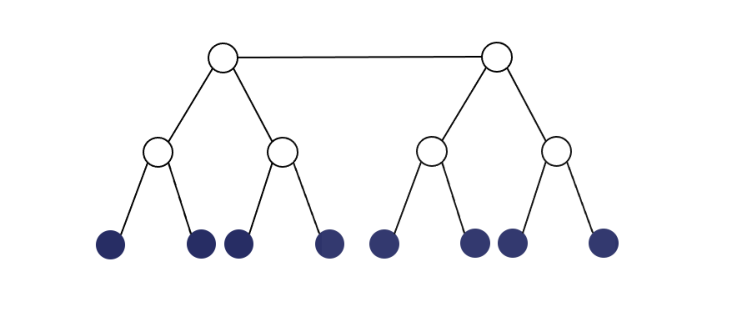
Refer to caption
(a) Double-binary tree
Refer to caption
(b) hmm
Refer to caption
(c) Full mm-tree, m=3m=3
Refer to caption
(d) Double star
Figure 5: Representative tree structures.

Appendix G Proofs of results in Section 3.1

Proof of Proposition 1.

For the sake of brevity, we prove the additivity property for paths of length 22. The proof for the general cases can be derived similarly. We consider the case xjx_{j} is on the path connected xix_{i} and xkx_{k} and xi,xj,xk∈𝒱x_{i},x_{j},x_{k}\in\mathcal{V}.

For any square matrix 𝐀∈ℝn×n\mathbf{A}\in\mathbb{R}^{n\times n}, the determinant of 𝐀\mathbf{A} is denoted as |𝐀|=det⁡(𝐀)|\mathbf{A}|=\mathrm{det}(\mathbf{A}).

Then we can write information distance as

d⁡(xi,xk)=−12​log⁡|𝚺i​k​𝚺i​k⊤​|+14​log⁡|𝚺i​i​𝚺i​i⊤|+14​log|​𝚺k​k​𝚺k​k⊤|\displaystyle\mathrm{d}(x_{i},x_{k})=-\frac{1}{2}\log\big|\mathbf{\Sigma}_{ik}\mathbf{\Sigma}_{ik}^{\top}\big|+\frac{1}{4}\log\big|\mathbf{\Sigma}_{ii}\mathbf{\Sigma}_{ii}^{\top}\big|+\frac{1}{4}\log\big|\mathbf{\Sigma}_{kk}\mathbf{\Sigma}_{kk}^{\top}\big| (G.1)

Note that 𝔼⁡[𝐱i|𝐱j]=𝚺i​j​𝚺j​j−1​𝐱j\mathbb{E}[\mathbf{x}_{i}|\mathbf{x}_{j}]=\mathbf{\Sigma}_{ij}\mathbf{\Sigma}_{jj}^{-1}\mathbf{x}_{j} and 𝚺i​j\mathbf{\Sigma}_{ij} is of full rank by Assumption 2, and

𝐀i|j=𝚺i​j​𝚺j​j−1\displaystyle\mathbf{A}_{i|j}=\mathbf{\Sigma}_{ij}\mathbf{\Sigma}_{jj}^{-1} (G.2)

is also of full rank.

Furthermore, we have

𝚺i​k=𝐀i|j​𝚺j​j​𝐀k|j⊤and𝚺i​k​𝚺i​k⊤=𝐀i|j​𝚺j​j​𝐀k|j⊤​𝐀k|j​𝚺j​j​𝐀i|j⊤.\displaystyle\mathbf{\Sigma}_{ik}=\mathbf{A}_{i|j}\mathbf{\Sigma}_{jj}\mathbf{A}_{k|j}^{\top}\quad\text{and}\quad\mathbf{\Sigma}_{ik}\mathbf{\Sigma}_{ik}^{\top}=\mathbf{A}_{i|j}\mathbf{\Sigma}_{jj}\mathbf{A}_{k|j}^{\top}\mathbf{A}_{k|j}\mathbf{\Sigma}_{jj}\mathbf{A}_{i|j}^{\top}. (G.3)

Then we have

|𝚺i​k​𝚺i​k⊤|\displaystyle\big|\mathbf{\Sigma}_{ik}\mathbf{\Sigma}_{ik}^{\top}\big| =|𝐀i|j​𝚺j​j​𝐀k|j⊤​𝐀k|j​𝚺j​j​𝐀i|j⊤|\displaystyle=\big|\mathbf{A}_{i|j}\mathbf{\Sigma}_{jj}\mathbf{A}_{k|j}^{\top}\mathbf{A}_{k|j}\mathbf{\Sigma}_{jj}\mathbf{A}_{i|j}^{\top}\big| (G.4)
=|𝐀i|j⊤​𝐀i|j​𝚺j​j​𝐀k|j⊤​𝐀k|j​𝚺j​j|\displaystyle=\big|\mathbf{A}_{i|j}^{\top}\mathbf{A}_{i|j}\mathbf{\Sigma}_{jj}\mathbf{A}_{k|j}^{\top}\mathbf{A}_{k|j}\mathbf{\Sigma}_{jj}\big| (G.5)
=|𝚺j​j⊤​𝐀i|j⊤​𝐀i|j​𝚺j​j||𝚺j​j|​|𝚺j​j⊤​𝐀k|j⊤​𝐀k|j​𝚺j​j||𝚺j​j|.\displaystyle=\frac{\big|\mathbf{\Sigma}_{jj}^{\top}\mathbf{A}_{i|j}^{\top}\mathbf{A}_{i|j}\mathbf{\Sigma}_{jj}\big|}{\big|\mathbf{\Sigma}_{jj}\big|}\frac{\big|\mathbf{\Sigma}_{jj}^{\top}\mathbf{A}_{k|j}^{\top}\mathbf{A}_{k|j}\mathbf{\Sigma}_{jj}\big|}{\big|\mathbf{\Sigma}_{jj}\big|}. (G.6)

Furthermore,

|𝚺j​j⊤​𝐀i|j⊤​𝐀i|j​𝚺j​j|\displaystyle\big|\mathbf{\Sigma}_{jj}^{\top}\mathbf{A}_{i|j}^{\top}\mathbf{A}_{i|j}\mathbf{\Sigma}_{jj}\big| =|𝐀i|j​𝚺j​j​𝚺j​j⊤​𝐀i|j⊤|=|𝚺i​j​𝚺i​j⊤|,\displaystyle=\big|\mathbf{A}_{i|j}\mathbf{\Sigma}_{jj}\mathbf{\Sigma}_{jj}^{\top}\mathbf{A}_{i|j}^{\top}\big|=\big|\mathbf{\Sigma}_{ij}\mathbf{\Sigma}_{ij}^{\top}\big|, (G.7)
|𝚺j​j⊤​𝐀k|j⊤​𝐀k|j​𝚺j​j|\displaystyle\big|\mathbf{\Sigma}_{jj}^{\top}\mathbf{A}_{k|j}^{\top}\mathbf{A}_{k|j}\mathbf{\Sigma}_{jj}\big| =|𝚺k​j​𝚺k​j⊤|.\displaystyle=\big|\mathbf{\Sigma}_{kj}\mathbf{\Sigma}_{kj}^{\top}\big|. (G.8)

Substituting (G.4) and (G.7) into (G.1), we have

d⁡(xi,xk)=\displaystyle\mathrm{d}(x_{i},x_{k})= −12​log⁡|𝚺i​j​𝚺i​j⊤|+14​log⁡|𝚺i​i​𝚺i​i⊤​|+14​log|​𝚺j​j​𝚺j​j⊤|\displaystyle-\frac{1}{2}\log\big|\mathbf{\Sigma}_{ij}\mathbf{\Sigma}_{ij}^{\top}\big|+\frac{1}{4}\log\big|\mathbf{\Sigma}_{ii}\mathbf{\Sigma}_{ii}^{\top}\big|+\frac{1}{4}\log\big|\mathbf{\Sigma}_{jj}\mathbf{\Sigma}_{jj}^{\top}\big|
−12​log⁡|𝚺k​j​𝚺k​j⊤|+14​log⁡|𝚺k​k​𝚺k​k⊤​|+14​log|​𝚺j​j​𝚺j​j⊤|\displaystyle\quad-\frac{1}{2}\log\big|\mathbf{\Sigma}_{kj}\mathbf{\Sigma}_{kj}^{\top}\big|+\frac{1}{4}\log\big|\mathbf{\Sigma}_{kk}\mathbf{\Sigma}_{kk}^{\top}\big|+\frac{1}{4}\log\big|\mathbf{\Sigma}_{jj}\mathbf{\Sigma}_{jj}^{\top}\big| (G.9)
=d⁡(xi,xj)+d⁡(xj,xk),\displaystyle=\mathrm{d}(x_{i},x_{j})+\mathrm{d}(x_{j},x_{k}), (G.10)

as desired. ∎

Lemma 8.

(Bernstein-type inequality [22]) Let X1,…,XnX_{1},\ldots,X_{n} be nn centered sub-exponential random variables, and K=max1≤i≤n⁡‖Xi‖ψ1K=\max_{1\leq i\leq n}\|X_{i}\|_{\psi_{1}}, where ∥⋅∥ψ1\|\cdot\|_{\psi_{1}} is the sub-exponential norm and is defined as

‖X‖ψ1:=supp≥1p−1​(𝔼​|X|p)1/p.\displaystyle\|X\|_{\psi_{1}}:=\sup_{p\geq 1}p^{-1}\big(\mathbb{E}|X|^{p}\big)^{1/p}. (G.11)

Then for every a=(a1,…,an)∈ℝna=(a_{1},\ldots,a_{n})\in\mathbb{R}^{n} and every t>0t>0, we have

ℙ⁡(|∑i=1nai​Xi|≥t)≤2​exp​[−c​min​{t2K2​‖a‖22,tK​‖a‖∞}]\displaystyle\mathbb{P}\bigg(\Big|\sum_{i=1}^{n}a_{i}X_{i}\Big|\geq t\bigg)\leq 2\exp\bigg[-c\min\Big\{\frac{t^{2}}{K^{2}\|a\|_{2}^{2}},\frac{t}{K\|a\|_{\infty}}\Big\}\bigg] (G.12)
Lemma 9.

Let the estimate of the covariance matrix 𝚺i​j\mathbf{\Sigma}_{ij} based on the truncated inner product be 𝚺^i​j\hat{\mathbf{\Sigma}}_{ij}. If t2<κ=max⁡{σmax2,ρmin}t_{2}<\kappa=\max\{\sigma_{\max}^{2},\rho_{\min}\}, we have

ℙ⁡(‖𝚺^i​j−𝚺i​j‖∞,∞>t1+t2)≤2​lmax2​e−3​n216​κ​n1​t1+lmax2​e−c​t22​n2κ2∀xi,xj∈𝒱obs.\displaystyle\mathbb{P}\big(\|\hat{\mathbf{\Sigma}}_{ij}-\mathbf{\Sigma}_{ij}\|_{\infty,\infty}>t_{1}+t_{2}\big)\leq 2l_{\max}^{2}e^{-\frac{3n_{2}}{16\kappa n_{1}}t_{1}}+l_{\max}^{2}e^{-c\frac{t_{2}^{2}n_{2}}{\kappa^{2}}}\quad\forall x_{i},x_{j}\in\mathcal{V}_{\mathrm{obs}}. (G.13)
Proof of Lemma 9.

Let Ii​j,1s​tI_{ij,1}^{st} be the set of indexes of the uncorrupted samples of [𝐱i]s​[𝐱j]t[\mathbf{x}_{i}]_{s}[\mathbf{x}_{j}]_{t}. Without loss of generality, we assume that |Ii​j,1s​t|=n2|I_{ij,1}^{st}|=n_{2}. Let Ii​j,2s​tI_{ij,2}^{st} and Ii​j,3s​tI_{ij,3}^{st} be the sets of the indexes of truncated uncorrupted samples and the reserved corrupted samples, respectively.

Refer to caption
Figure 6: Illustration of the truncated inner product.

Then,

[𝚺^i​j]s​t=1n2​(∑m∈Ii​j,1s​t[𝐱i]s(m)​[𝐱j]t(m)−∑m∈Ii​j,2s​t[𝐱i]s(m)​[𝐱j]t(m)+∑m∈Ii​j,3s​t[𝐱i]s(m)​[𝐱j]t(m))\displaystyle[\hat{\mathbf{\Sigma}}_{ij}]_{st}=\frac{1}{n_{2}}\bigg(\sum_{m\in I_{ij,1}^{st}}[\mathbf{x}_{i}]_{s}^{(m)}[\mathbf{x}_{j}]_{t}^{(m)}-\sum_{m\in I_{ij,2}^{st}}[\mathbf{x}_{i}]_{s}^{(m)}[\mathbf{x}_{j}]_{t}^{(m)}+\sum_{m\in I_{ij,3}^{st}}[\mathbf{x}_{i}]_{s}^{(m)}[\mathbf{x}_{j}]_{t}^{(m)}\bigg) (G.14)

The (s,t)th(s,t)^{\mathrm{th}} entry of the error covariance matrix 𝚺~i​j=𝚺^i​j−𝚺i​j∈ℝd×d\tilde{\mathbf{\Sigma}}_{ij}=\hat{\mathbf{\Sigma}}_{ij}-\mathbf{\Sigma}_{ij}\in\mathbb{R}^{d\times d} is defined as

[𝚺~i​j]s​t=1n2(−∑m∈Ii​j,2s​t[𝐱i]s(m)[𝐱j]t(m)+∑m∈Ii​j,3s​t[𝐱i]s(m)[𝐱j]t(m)).\displaystyle[\tilde{\mathbf{\Sigma}}_{ij}]_{st}=\frac{1}{n_{2}}\bigg(-\sum_{m\in I_{ij,2}^{st}}[\mathbf{x}_{i}]_{s}^{(m)}[\mathbf{x}_{j}]_{t}^{(m)}+\sum_{m\in I_{ij,3}^{st}}[\mathbf{x}_{i}]_{s}^{(m)}[\mathbf{x}_{j}]_{t}^{(m)}\bigg). (G.15)

From the definition of the truncated inner product, we can bound the right-hand side of (G.15) as

|[𝚺~i​j]s​t|≤2n2​∑m∈Ii​j,2s​t|[𝐱i]s(m)​[𝐱j]t(m)|.\displaystyle\big|[\tilde{\mathbf{\Sigma}}_{ij}]_{st}\big|\leq\frac{2}{n_{2}}\sum_{m\in I_{ij,2}^{st}}\big|[\mathbf{x}_{i}]_{s}^{(m)}[\mathbf{x}_{j}]_{t}^{(m)}\big|. (G.16)

Equipped with the expression of the moment-generating function of a chi-squared distribution, the moment-generating function of each term in the sum of (G.16) can be upper bounded as

𝔼⁡[eλ​|[𝐱i]s(m)​[𝐱j]t(m)|]\displaystyle\mathbb{E}\Big[e^{\lambda|[\mathbf{x}_{i}]_{s}^{(m)}[\mathbf{x}_{j}]_{t}^{(m)}|}\Big] ≤𝔼⁡[eλ​([𝐱i]s(m))2+([𝐱j]t(m))22]\displaystyle\leq\mathbb{E}\Big[e^{\lambda\frac{([\mathbf{x}_{i}]_{s}^{(m)})^{2}+([\mathbf{x}_{j}]_{t}^{(m)})^{2}}{2}}\Big] (G.17)
≤𝔼⁡[eλ​([𝐱i]s(m))2]​𝔼​[eλ​([𝐱j]t(m))2]\displaystyle\leq\sqrt{\mathbb{E}\big[e^{\lambda([\mathbf{x}_{i}]_{s}^{(m)})^{2}}\big]\mathbb{E}\big[e^{\lambda([\mathbf{x}_{j}]_{t}^{(m)})^{2}}\big]} (G.18)
≤11−2​σmax2​λ.\displaystyle\leq\frac{1}{\sqrt{1-2\sigma_{\max}^{2}\lambda}}. (G.19)

Using the power mean inequality, we have

(e2​λn2​∑m∈Ii​j,2s​t|[𝐱i]s(m)​[𝐱j]t(m)|)1|Ii​j,2s​t|\displaystyle\Big(e^{\frac{2\lambda}{n_{2}}\sum_{m\in I_{ij,2}^{st}}|[\mathbf{x}_{i}]_{s}^{(m)}[\mathbf{x}_{j}]_{t}^{(m)}|}\Big)^{\frac{1}{|I_{ij,2}^{st}|}} ≤∑m∈Ii​j,2s​te2​λn2​|[𝐱i]s(m)​[𝐱j]t(m)||Ii​j,2s​t|\displaystyle\leq\frac{\sum_{m\in I_{ij,2}^{st}}e^{\frac{2\lambda}{n_{2}}|[\mathbf{x}_{i}]_{s}^{(m)}[\mathbf{x}_{j}]_{t}^{(m)}|}}{|I_{ij,2}^{st}|} (G.20)
≤(∑m∈Ii​j,2s​te2​λ​n1n2​|[𝐱i]s(m)​[𝐱j]t(m)||Ii​j,2s​t|)1n1.\displaystyle\leq\bigg(\frac{\sum_{m\in I_{ij,2}^{st}}e^{\frac{2\lambda n_{1}}{n_{2}}|[\mathbf{x}_{i}]_{s}^{(m)}[\mathbf{x}_{j}]_{t}^{(m)}|}}{|I_{ij,2}^{st}|}\bigg)^{\frac{1}{n_{1}}}. (G.21)

Thus,

𝔼⁡[eλ​|[𝚺~i​j]s​t|]\displaystyle\mathbb{E}\Big[e^{\lambda|[\tilde{\mathbf{\Sigma}}_{ij}]_{st}|}\Big] ≤𝔼⁡[e2​λn2​∑m∈Ii​j,2s​t|[𝐱i]s(m)​[𝐱j]t(m)|]≤maxm∈Ii​j,2s​t⁡𝔼⁡[e2​λ​n1n2​|[𝐱i]s(m)​[𝐱j]t(m)|]\displaystyle\leq\mathbb{E}\Big[e^{\frac{2\lambda}{n_{2}}\sum_{m\in I_{ij,2}^{st}}\big|[\mathbf{x}_{i}]_{s}^{(m)}[\mathbf{x}_{j}]_{t}^{(m)}\big|}\Big]\leq\max_{m\in I_{ij,2}^{st}}\mathbb{E}\Big[e^{\frac{2\lambda n_{1}}{n_{2}}\big|[\mathbf{x}_{i}]_{s}^{(m)}[\mathbf{x}_{j}]_{t}^{(m)}\big|}\Big] (G.22)
≤11−4​σmax2​n1n2​λ\displaystyle\leq\frac{1}{\sqrt{1-\frac{4\sigma_{\max}^{2}n_{1}}{n_{2}}\lambda}} (G.23)

and

𝔼⁡[eλ​maxs,t​|[𝚺~i​j]s​t|]\displaystyle\mathbb{E}\Big[e^{\lambda\max_{s,t}\big|[\tilde{\mathbf{\Sigma}}_{ij}]_{st}\big|}\Big] =𝔼⁡[maxs,t⁡eλ​|[𝚺~i​j]s​t|]≤lmax2​𝔼​[eλ​|[𝚺~i​j]s​t|]≤lmax21−4​σmax2​n1n2​λ.\displaystyle=\mathbb{E}\Big[\max_{s,t}e^{\lambda\big|[\tilde{\mathbf{\Sigma}}_{ij}]_{st}\big|}\Big]\leq l_{\max}^{2}\mathbb{E}\Big[e^{\lambda\big|[\tilde{\mathbf{\Sigma}}_{ij}]_{st}\big|}\Big]\leq\frac{l_{\max}^{2}}{\sqrt{1-\frac{4\sigma_{\max}^{2}n_{1}}{n_{2}}\lambda}}. (G.24)

Thus,

ℙ⁡(‖𝚺~i​j‖∞,∞>t)\displaystyle\mathbb{P}\big(\|\tilde{\mathbf{\Sigma}}_{ij}\|_{\infty,\infty}>t\big) =ℙ⁡(maxs,t⁡|[𝚺~i​j]s​t|>t)=ℙ⁡(eλ​maxs,t​|[𝚺~i​j]s​t|>eλ​t)\displaystyle=\mathbb{P}\Big(\max_{s,t}\big|[\tilde{\mathbf{\Sigma}}_{ij}]_{st}\big|>t\Big)=\mathbb{P}\Big(e^{\lambda\max_{s,t}\big|[\tilde{\mathbf{\Sigma}}_{ij}]_{st}\big|}>e^{\lambda t}\Big) (G.25)
≤e−λ​t​𝔼​[eλ​maxs,t​|[𝚺~i​j]s​t|]≤e−λ​t​lmax21−4​σmax2​n1n2​λ.\displaystyle\leq e^{-\lambda t}\mathbb{E}\Big[e^{\lambda\max_{s,t}\big|[\tilde{\mathbf{\Sigma}}_{ij}]_{st}\big|}\Big]\leq e^{-\lambda t}\frac{l_{\max}^{2}}{\sqrt{1-\frac{4\sigma_{\max}^{2}n_{1}}{n_{2}}\lambda}}. (G.26)

Let λ=3​n216​σmax2​n1\lambda=\frac{3n_{2}}{16\sigma_{\max}^{2}n_{1}}, then we have

ℙ⁡(‖𝚺~i​j‖∞,∞>t)≤2​lmax2​e−3​n216​σmax2​n1​t.\displaystyle\mathbb{P}\big(\|\tilde{\mathbf{\Sigma}}_{ij}\|_{\infty,\infty}>t\big)\leq 2l_{\max}^{2}e^{-\frac{3n_{2}}{16\sigma_{\max}^{2}n_{1}}t}. (G.27)

According to Lemma 8 (since the involved random variables are sub-exponential), we have

ℙ⁡(|1n2​∑m∈Ii​j,1s​t([𝐱i]s(m)​[𝐱j]t(m)−[𝚺i​j]s​t)|>t)≤exp⁡(−c​min⁡{t2​n2K2,t​n2K}),\displaystyle\mathbb{P}\bigg(\Big|\frac{1}{n_{2}}\sum_{m\in I_{ij,1}^{st}}\big([\mathbf{x}_{i}]_{s}^{(m)}[\mathbf{x}_{j}]_{t}^{(m)}-[\mathbf{\Sigma}_{ij}]_{st}\big)\Big|>t\bigg)\leq\exp\bigg(-c\min\Big\{\frac{t^{2}n_{2}}{K^{2}},\frac{tn_{2}}{K}\Big\}\bigg), (G.28)

where K=σmax2K=\sigma_{\max}^{2}.

Thus, if t<κt<\kappa, we have

ℙ⁡(‖𝚺^i​j−𝚺i​j‖∞,∞>t1+t2)≤2​lmax2​e−3​n216​κ​n1​t1+lmax2​e−c​t22​n2κ2,\displaystyle\mathbb{P}\big(\|\hat{\mathbf{\Sigma}}_{ij}-\mathbf{\Sigma}_{ij}\|_{\infty,\infty}>t_{1}+t_{2}\big)\leq 2l_{\max}^{2}e^{-\frac{3n_{2}}{16\kappa n_{1}}t_{1}}+l_{\max}^{2}e^{-c\frac{t_{2}^{2}n_{2}}{\kappa^{2}}}, (G.29)

as desired. ∎

Proof of Proposition  2.

From the definition of the information distance, we have

d(xi,xj)=−∑n=1lmaxlogσn(𝚺i​j)+12logdet(𝚺i​i)+12logdet(𝚺j​j).\displaystyle\mathrm{d}(x_{i},x_{j})=-\sum_{n=1}^{l_{\max}}\log\sigma_{n}\big(\mathbf{\Sigma}_{ij}\big)+\frac{1}{2}\log\det\big(\mathbf{\Sigma}_{ii}\big)+\frac{1}{2}\log\det\big(\mathbf{\Sigma}_{jj}\big). (G.30)

According to the inequality ‖𝐀‖2≤‖𝐀‖1​‖𝐀‖∞\|\mathbf{A}\|_{2}\leq\sqrt{\|\mathbf{A}\|_{1}\|\mathbf{A}\|_{\infty}} which holds for all 𝐀∈ℝn×m\mathbf{A}\in\mathbb{R}^{n\times m} [23], we have

|σk​(𝚺^i​j)−σk​(𝚺i​j)|\displaystyle\big|\sigma_{k}(\hat{\mathbf{\Sigma}}_{ij})-\sigma_{k}(\mathbf{\Sigma}_{ij})\big| ≤‖𝚺^i​j−𝚺i​j‖2\displaystyle\leq\|\hat{\mathbf{\Sigma}}_{ij}-\mathbf{\Sigma}_{ij}\|_{2} (G.31)
≤‖𝚺^i​j−𝚺i​j‖∞​‖𝚺^i​j−𝚺i​j‖1≤lmax​‖𝚺^i​j−𝚺i​j‖∞,∞.\displaystyle\leq\sqrt{\|\hat{\mathbf{\Sigma}}_{ij}-\mathbf{\Sigma}_{ij}\|_{\infty}\|\hat{\mathbf{\Sigma}}_{ij}-\mathbf{\Sigma}_{ij}\|_{1}}\leq l_{\max}\|\hat{\mathbf{\Sigma}}_{ij}-\mathbf{\Sigma}_{ij}\|_{\infty,\infty}. (G.32)

Using the triangle inequality, we arrive at

|d^​(xi,xj)−d⁡(xi,xj)|≤\displaystyle\big|\hat{\mathrm{d}}(x_{i},x_{j})-\mathrm{d}(x_{i},x_{j})\big|\leq ∑n=1lmax|log⁡σn​(𝚺^i​j)−log⁡σn​(𝚺i​j)|+12​∑n=1dim⁡(𝐱i)|log⁡σn​(𝚺^i​i)−log⁡σn​(𝚺i​i)|\displaystyle\sum_{n=1}^{l_{\max}}\big|\log\sigma_{n}(\hat{\mathbf{\Sigma}}_{ij})-\log\sigma_{n}(\mathbf{\Sigma}_{ij})\big|+\frac{1}{2}\sum_{n=1}^{\mathrm{dim}(\mathbf{x}_{i})}\big|\log\sigma_{n}(\hat{\mathbf{\Sigma}}_{ii})-\log\sigma_{n}(\mathbf{\Sigma}_{ii})\big|
+12∑n=1dim⁡(𝐱j)|logσn(𝚺^j​j)−logσn(𝚺j​j)|.\displaystyle+\frac{1}{2}\sum_{n=1}^{\mathrm{dim}(\mathbf{x}_{j})}\big|\log\sigma_{n}(\hat{\mathbf{\Sigma}}_{jj})-\log\sigma_{n}(\mathbf{\Sigma}_{jj})\big|. (G.33)

Furthermore, since the singular value is lower bounded by γmin\gamma_{\min}, using Taylor’s theorem and (G.31), we obtain

|log⁡σn​(𝚺^i​j)−log⁡σn​(𝚺i​j)|≤1γmin​|σn​(𝚺^i​j)−σn​(𝚺i​j)|≤lmaxγmin​‖𝚺^i​j−𝚺i​j‖∞,∞.\displaystyle\big|\log\sigma_{n}(\hat{\mathbf{\Sigma}}_{ij})-\log\sigma_{n}(\mathbf{\Sigma}_{ij})\big|\leq\frac{1}{\gamma_{\min}}\big|\sigma_{n}(\hat{\mathbf{\Sigma}}_{ij})-\sigma_{n}(\mathbf{\Sigma}_{ij})\big|\leq\frac{l_{\max}}{\gamma_{\min}}\|\hat{\mathbf{\Sigma}}_{ij}-\mathbf{\Sigma}_{ij}\|_{\infty,\infty}. (G.34)

Finally,

|d^​(xi,xj)−d⁡(xi,xj)|\displaystyle\big|\hat{\mathrm{d}}(x_{i},x_{j})-\mathrm{d}(x_{i},x_{j})\big| ≤(lmax+dim⁡(𝐱i)+dim⁡(𝐱j)2)​lmaxγmin​‖𝚺^i​j−𝚺i​j‖∞,∞\displaystyle\leq\Big(l_{\max}+\frac{\mathrm{dim}(\mathbf{x}_{i})+\mathrm{dim}(\mathbf{x}_{j})}{2}\Big)\frac{l_{\max}}{\gamma_{\min}}\|\hat{\mathbf{\Sigma}}_{ij}-\mathbf{\Sigma}_{ij}\|_{\infty,\infty}
≤2​lmax2γmin​‖𝚺^i​j−𝚺i​j‖∞,∞.\displaystyle\leq\frac{2l_{\max}^{2}}{\gamma_{\min}}\|\hat{\mathbf{\Sigma}}_{ij}-\mathbf{\Sigma}_{ij}\|_{\infty,\infty}. (G.35)

From Lemma 9, the proposition is proved. ∎

Appendix H Proofs of results in Section 3.2

Lemma 10.

Consider the optimization problem

𝒫:max{xi}\displaystyle\mathscr{P}:\quad\max\limits_{\{x_{i}\}}\quad f⁡(𝐱)=∑i=1nxi​(xi−1)\displaystyle f(\mathbf{x})=\sum_{i=1}^{n}x_{i}(x_{i}-1)
s.t.\displaystyle{\rm s.t.}\quad ∑i=1Nxi≤N0≤xi≤ki=1,…,N.\displaystyle\sum_{i=1}^{N}x_{i}\leq N\quad 0\leq x_{i}\leq k\qquad i=1,\ldots,N. (H.1)

Assume n​k≥Nnk\geq N. An optimal solution is given by xi=kx_{i}=k for all i=1,…,⌊Nk⌋i=1,\ldots,\lfloor\frac{N}{k}\rfloor and x⌊Nk⌋+1=N−k⁡⌊Nk⌋x_{\lfloor\frac{N}{k}\rfloor+1}=N-k\lfloor\frac{N}{k}\rfloor, and xi=0x_{i}=0 for i=⌊Nk⌋+2,…,ni=\lfloor\frac{N}{k}\rfloor+2,\ldots,n.

This lemma can be verified by direct calculation, and so we will omit the details.

Proof of Proposition 4.

We prove the proposition by induction.

Proposition 2 and Eqn. (6) show that at the 0th0^{\mathrm{th}} layer [24]

ℙ⁡(|Δi​j|>ε)<f⁡(ε)=h(0)​(ε).\displaystyle\mathbb{P}(|\Delta_{ij}|>\varepsilon)<f(\varepsilon)=h^{(0)}(\varepsilon). (H.2)

Now suppose that the distances related to the nodes created in the (l−1)st(l-1)^{\mathrm{st}} iteration satisfy

ℙ⁡(|d^​(xi,xh)−d⁡(xi,xh)|>ε)<h(l−1)​(ε).\displaystyle\mathbb{P}\Big(\big|\hat{\mathrm{d}}(x_{i},x_{h})-\mathrm{d}(x_{i},x_{h})\big|>\varepsilon\Big)<h^{(l-1)}(\varepsilon). (H.3)

Since s>1s>1 and m<1m<1, it is obvious that

h(l)​(ε)≤h(l+k)​(ε)for alll,k∈ℕ and for allε>0.\displaystyle h^{(l)}(\varepsilon)\leq h^{(l+k)}(\varepsilon)\quad\mbox{for all}\quad l,k\in\mathbb{N}\quad\text{ and for all}\quad\varepsilon>0. (H.4)

Then we can deduce that

ℙ⁡(|d^​(xi,xj)−d⁡(xi,xj)|>ε)<h(l−1)​(ε)for allxi,xj∈Γl.\displaystyle\mathbb{P}(|\hat{\mathrm{d}}(x_{i},x_{j})-\mathrm{d}(x_{i},x_{j})|>\varepsilon)<h^{(l-1)}(\varepsilon)\quad\mbox{for all}\quad x_{i},x_{j}\in\Gamma^{l}. (H.5)

From the update equation of the distance in (9), we have

d^​(xi,xh)\displaystyle\hat{\mathrm{d}}(x_{i},x_{h}) =12​(|𝒞​(h)−1|)​(∑j∈𝒞⁡(h)(d⁡(xi,xj)+Δi​j)+1|𝒦i​j|​∑k∈𝒦i​j(Φi​j​k+Δi​k−Δj​k))\displaystyle=\frac{1}{2(\big|\mathcal{C}(h)-1|\big)}\bigg(\sum_{j\in\mathcal{C}(h)}(\mathrm{d}(x_{i},x_{j})+\Delta_{ij})+\frac{1}{|\mathcal{K}_{ij}|}\sum_{k\in\mathcal{K}_{ij}}(\Phi_{ijk}+\Delta_{ik}-\Delta_{jk})\bigg) (H.6)

and

d^​(xi,xh)\displaystyle\hat{\mathrm{d}}(x_{i},x_{h}) =12​(|𝒞​(h)−1|)​(∑j∈𝒞⁡(h)Δi​j+1|𝒦i​j|​∑k∈𝒦i​j(Δi​k−Δj​k))+d⁡(xi,xh).\displaystyle=\frac{1}{2(\big|\mathcal{C}(h)-1|\big)}\bigg(\sum_{j\in\mathcal{C}(h)}\Delta_{ij}+\frac{1}{|\mathcal{K}_{ij}|}\sum_{k\in\mathcal{K}_{ij}}(\Delta_{ik}-\Delta_{jk})\bigg)+\mathrm{d}(x_{i},x_{h}). (H.7)

Using the union bound, we find that

ℙ⁡(|d^​(xi,xh)−d⁡(xi,xh)|>ε)\displaystyle\mathbb{P}\Big(\big|\hat{\mathrm{d}}(x_{i},x_{h})-\mathrm{d}(x_{i},x_{h})\big|>\varepsilon\Big)
≤ℙ(⋃j∈𝒞⁡(h){|Δi​j+1|𝒦i​j|∑k∈𝒦i​j(Δi​k−Δj​k)|>2ε})\displaystyle\leq\mathbb{P}\bigg(\bigcup_{j\in\mathcal{C}(h)}\Big\{\big|\Delta_{ij}+\frac{1}{|\mathcal{K}_{ij}|}\sum_{k\in\mathcal{K}_{ij}}(\Delta_{ik}-\Delta_{jk})\big|>2\varepsilon\Big\}\bigg) (H.8)
≤∑j∈𝒞⁡(h)ℙ⁡(|Δi​j+1|𝒦i​j|​∑k∈𝒦i​j(Δi​k−Δj​k)|>2​ε)\displaystyle\leq\sum_{j\in\mathcal{C}(h)}\mathbb{P}\bigg(\big|\Delta_{ij}+\frac{1}{|\mathcal{K}_{ij}|}\sum_{k\in\mathcal{K}_{ij}}(\Delta_{ik}-\Delta_{jk})\big|>2\varepsilon\bigg) (H.9)
≤∑j∈𝒞⁡(h)[ℙ⁡(|Δi​j|>23​ε)+∑k∈𝒦i​jℙ⁡(|Δi​k|>23​ε)+ℙ⁡(|Δj​k|>23​ε)].\displaystyle\leq\sum_{j\in\mathcal{C}(h)}\bigg[\mathbb{P}\Big(|\Delta_{ij}|>\frac{2}{3}\varepsilon\Big)+\sum_{k\in\mathcal{K}_{ij}}\mathbb{P}\Big(|\Delta_{ik}|>\frac{2}{3}\varepsilon\Big)+\mathbb{P}\Big(|\Delta_{jk}|>\frac{2}{3}\varepsilon\Big)\bigg]. (H.10)

The estimates of the distances related to the nodes in the lthl^{\mathrm{th}} layer satisfy

ℙ⁡(|d^​(xi,xh)−d⁡(xi,xh)|>ε)\displaystyle\mathbb{P}\Big(\big|\hat{\mathrm{d}}(x_{i},x_{h})-\mathrm{d}(x_{i},x_{h})\big|>\varepsilon\Big) <|𝒞⁡(h)|(1+2​|𝒦i​j|)​h(l−1)​(23​ε)\displaystyle<|\mathcal{C}(h)|\big(1+2|\mathcal{K}_{ij}|\big)h^{(l-1)}\big(\frac{2}{3}\varepsilon\big) (H.11)
≤dmax​(1+2​Nτ)​h(l−1)​(23​ε).\displaystyle\leq d_{\max}(1+2N_{\tau})h^{(l-1)}\big(\frac{2}{3}\varepsilon\big). (H.12)

Similarly, from (3.2), we have

ℙ⁡(|d^​(xk,xh)−d⁡(xk,xh)|>ε)\displaystyle\mathbb{P}\Big(\big|\hat{\mathrm{d}}(x_{k},x_{h})-\mathrm{d}(x_{k},x_{h})\big|>\varepsilon\Big)
≤{∑i∈𝒞⁡(h)ℙ⁡(|Δi​k|>12​ε)+ℙ⁡(|Δi​h|>12​ε),if ​k∈𝒱obs∑(i,j)∈𝒞⁡(h)×𝒞⁡(k)ℙ⁡(|Δi​j|>13​ε)+ℙ⁡(|Δi​h|>13​ε)+ℙ⁡(|Δj​k|>13​ε),otherwise.\displaystyle\leq\left\{\begin{array}[]{lr}\sum_{i\in\mathcal{C}(h)}\mathbb{P}\big(|\Delta_{ik}|>\frac{1}{2}\varepsilon\big)+\mathbb{P}\big(|\Delta_{ih}|>\frac{1}{2}\varepsilon\big),&\text{if }k\in\mathcal{V}_{\mathrm{obs}}\\ \sum_{(i,j)\in\mathcal{C}(h)\times\mathcal{C}(k)}\mathbb{P}\big(|\Delta_{ij}|>\frac{1}{3}\varepsilon\big)+\mathbb{P}\big(|\Delta_{ih}|>\frac{1}{3}\varepsilon\big)+\mathbb{P}\big(|\Delta_{jk}|>\frac{1}{3}\varepsilon\big),&\text{otherwise.}\end{array}\right.

Using the concentration bound at the (l−1)st(l-1)^{\mathrm{st}} layer in inequality (H.3), we have

ℙ(|d^(xk,xh)\displaystyle\mathbb{P}\Big(\big|\hat{\mathrm{d}}(x_{k},x_{h}) OPEN−d⁡(xk,xh)|>ε)\displaystyle-\mathrm{d}(x_{k},x_{h})\big|>\varepsilon\Big)
≤{dmax​h(l−1)​(12​ε)+dmax2​(1+2​Nτ)​h(l−1)​(13​ε),if ​k∈𝒱obsdmax2​h(l−1)​(23​ε)+2​dmax3​(1+2​Nτ)​h(l−1)​(29​ε),otherwise.\displaystyle\leq\left\{\begin{array}[]{lr}d_{\max}h^{(l-1)}(\frac{1}{2}\varepsilon)+d_{\max}^{2}(1+2N_{\tau})h^{(l-1)}(\frac{1}{3}\varepsilon),&\text{if }k\in\mathcal{V}_{\mathrm{obs}}\\ d_{\max}^{2}h^{(l-1)}(\frac{2}{3}\varepsilon)+2d_{\max}^{3}(1+2N_{\tau})h^{(l-1)}(\frac{2}{9}\varepsilon),&\text{otherwise.}\end{array}\right.

Summarizing the above three concentration bounds, we have that for the nodes at the lthl^{\mathrm{th}} layer, estimates of the information distances (based on the truncated inner product) satisfy

ℙ(|d^(xk,xh)\displaystyle\mathbb{P}\Big(\big|\hat{\mathrm{d}}(x_{k},x_{h}) OPEN−d⁡(xk,xh)|>ε)<[dmax2+2​dmax3​(1+2​Nτ)]​h(l−1)​(29​ε)=h(l)​(ε).\displaystyle-\mathrm{d}(x_{k},x_{h})\big|>\varepsilon\Big)<\big[d_{\max}^{2}+2d_{\max}^{3}(1+2N_{\tau})\big]h^{(l-1)}\Big(\frac{2}{9}\varepsilon\Big)=h^{(l)}(\varepsilon). (H.17)

∎

Proposition 11.

The cardinalities of the active sets in lthl^{\mathrm{th}} and (l+1)st(l+1)^{\mathrm{st}} iterations admit following relationship

|Γl|dmax≤|Γl+1|≤|Γl|−2.\displaystyle\frac{|\Gamma^{l}|}{d_{\max}}\leq|\Gamma^{l+1}|\leq|\Gamma^{l}|-2. (H.18)
Proof of Proposition  11.

Note that at the lthl^{\mathrm{th}} iteration, the number of families is |Γl+1||\Gamma^{l+1}|, and thus we have

∑i=1|Γl+1|ni=|Γl|,\displaystyle\sum_{i=1}^{|\Gamma^{l+1}|}n_{i}=|\Gamma^{l}|, (H.19)

where nin_{i} is the number of nodes in Γl\Gamma^{l} in each family. Since 1≤ni≤dmax1\leq n_{i}\leq d_{\max}, we have Γldmax≤|Γl+1|\frac{\Gamma^{l}}{d_{\max}}\leq|\Gamma^{l+1}|.

Refer to caption
Figure 7: Illustration of rrg. The shaded nodes are the observed nodes and the rest are hidden nodes. Γ1={x1,x2,…,,x9}\Gamma^{1}=\{x_{1},x_{2},\ldots,,x_{9}\}, and Γ2\Gamma^{2} is the nodes in the dotted lines. If we delete the nodes in Γ2\Gamma^{2}, the remained unknown hidden nodes are x10x_{10}, x11x_{11} and x13x_{13}. Nodes x10x_{10} and x13x_{13} are at the end of the chain formed by these two nodes, and x11x_{11} is at the end of the degenerate chain formed by itself.

We next prove that there are at least two of nin_{i}’s not less than 22. If we delete the nodes in active set Γl\Gamma^{l}, the remaining hidden nodes form a single tree or a forest. There will at least two nodes at the end of the chain, which means that they only have one neighbor in hidden nodes, as shown in Fig. 7. Since they at least have three neighbors, they have at least two neighbors in Γl\Gamma^{l}. Thus, there are at least two of nin_{i}’s not less than 2, and thus |Γl+1|≤|Γl|−2|\Gamma^{l+1}|\leq|\Gamma^{l}|-2. ∎

Corollary 1.

The maximum number of iterations of Algorithm 1, LRL_{\mathrm{R}}, is bounded as

log⁡|𝒱obs|2log⁡dmax≤LR≤|𝒱obs|−2.\displaystyle\frac{\log\frac{|\mathcal{V}_{\mathrm{obs}}|}{2}}{\log d_{\max}}\leq L_{\mathrm{R}}\leq|\mathcal{V}_{\mathrm{obs}}|-2. (H.20)
Proof.

When Algorithm 1 terminates, |Γ|≤2|\Gamma|\leq 2. Combining Proposition 11 and |Γ|≤2|\Gamma|\leq 2 proves the corollary. ∎

Theorem 6.

Under Assumptions 1–5, rrg algorithm constructs the correct latent tree with probability at least 1−η1-\eta if

n2\displaystyle n_{2} ≥64​λ2​κ2c​ε2​(92)2​LR−2​log⁡17​lmax2​sLR−1​|𝒱obs|3η\displaystyle\geq\frac{64\lambda^{2}\kappa^{2}}{c\varepsilon^{2}}\big(\frac{9}{2}\big)^{2L_{\mathrm{R}}-2}\log\frac{17l_{\max}^{2}s^{L_{\mathrm{R}}-1}|\mathcal{V}_{\mathrm{obs}}|^{3}}{\eta} (H.21)
n2n1\displaystyle\frac{n_{2}}{n_{1}} ≥128​λ​κ3​ε​(92)LR−1​log⁡34​lmax2​sLR−1​|𝒱obs|3η,\displaystyle\geq\frac{128\lambda\kappa}{3\varepsilon}\big(\frac{9}{2}\big)^{L_{\mathrm{R}}-1}\log\frac{34l_{\max}^{2}s^{L_{\mathrm{R}}-1}|\mathcal{V}_{\mathrm{obs}}|^{3}}{\eta}, (H.22)

where

λ=2​lmax2​eρmax/lmaxδmin1/lmaxκ=max⁡{σmax2,ρmin}s=dmax2+2​dmax3​(1+2​Nτ)ε=ρmin2,\displaystyle\lambda=\frac{2l_{\max}^{2}e^{\rho_{\max}/l_{\max}}}{\delta_{\min}^{1/l_{\max}}}\quad\kappa=\max\{\sigma_{\max}^{2},\rho_{\min}\}\quad s=d_{\max}^{2}+2d_{\max}^{3}(1+2N_{\tau})\quad\varepsilon=\frac{\rho_{\min}}{2}, (H.23)

cc is an absolute constant, and LRL_{\mathrm{R}} is the number of iterations of rrg needed to construct the tree.

Proof of Theorem  6.

It is easy to see by substituting the constants λ\lambda, κ\kappa, ss and ε\varepsilon into (H.21) and (H.22) that Theorem 6 implies Theorem 1, so we provide the proof of Theorem 6 here.

The error events of learning structure in the lthl^{\mathrm{th}} layer of the latent tree (the 0th0^{\mathrm{th}} layer consists of the observed nodes, and the (l+1)st(l+1)^{\mathrm{st}} layer is the active set formed from lthl^{\mathrm{th}} layer). The error events could be enumerated as: misclassification of families ℰfl\mathcal{E}^{l}_{\mathrm{f}}, misclassification of non-families ℰnfl\mathcal{E}^{l}_{\mathrm{nf}}, misclassification of parents ℰpl\mathcal{E}^{l}_{\mathrm{p}} and misclassification of siblings ℰsl\mathcal{E}^{l}_{\mathrm{s}}. We will bound the probabilities of these four error events in the following.

The event representing misclassification of families ℰfl\mathcal{E}^{l}_{\mathrm{f}} represents classifying the nodes that are not in the same family as a family. Suppose nodes xix_{i} and xjx_{j} are in different families. The event that classifying them to be in the same family ℰf,i​jl\mathcal{E}^{l}_{\mathrm{f},ij} at layer ll can be expressed as

ℰf,i​jl={|Φ^i​j​k−Φ^i​j​k′|<εfor allxk,xk′∈Γl}.\displaystyle\mathcal{E}^{l}_{\mathrm{f},ij}=\big\{|\hat{\Phi}_{ijk}-\hat{\Phi}_{ijk^{\prime}}|<\varepsilon\quad\text{for all}\quad x_{k},x_{k^{\prime}}\in\Gamma^{l}\big\}. (H.24)

We have

ℙ⁡(ℰf,i​jl)\displaystyle\mathbb{P}(\mathcal{E}^{l}_{\mathrm{f},ij}) =ℙ(⋂xk,xk′∈Γ{|Φ^i​j​k−Φ^i​j​k′|<ε})≤minxk,xk′∈Γℙ(|Φ^i​j​k−Φ^i​j​k′|<ε),\displaystyle=\mathbb{P}\Big(\bigcap_{x_{k},x_{k^{\prime}}\in\Gamma}\big\{|\hat{\Phi}_{ijk}-\hat{\Phi}_{ijk^{\prime}}|<\varepsilon\big\}\Big)\leq\min_{x_{k},x_{k^{\prime}}\in\Gamma}\mathbb{P}\Big(|\hat{\Phi}_{ijk}-\hat{\Phi}_{ijk^{\prime}}|<\varepsilon\Big), (H.25)
ℙ⁡(ℰfl)\displaystyle\mathbb{P}(\mathcal{E}^{l}_{\mathrm{f}}) =ℙ⁡(⋃xi,xj​not in same familyℰf,i​jl)=ℙ⁡(⋃(xi,xj)∈Γflℰf,i​jl).\displaystyle=\mathbb{P}\Big(\bigcup_{x_{i},x_{j}\text{not in same family}}\mathcal{E}^{l}_{\mathrm{f},ij}\Big)=\mathbb{P}\Big(\bigcup_{(x_{i},x_{j})\in\Gamma^{l}_{\mathrm{f}}}\mathcal{E}^{l}_{\mathrm{f},ij}\Big). (H.26)

We enumerate all possible structural relationships between xix_{i}, xjx_{j}, xkx_{k} and xk′x_{k^{\prime}}

Refer to caption
Figure 8: Enumerating of four-node topology and the corresponding |Φi​j​k−Φi​j​k′||\Phi_{ijk}-\Phi_{ijk^{\prime}}|.

Let ε<2​ρmin\varepsilon<2\rho_{\min}, by decomposing the estimate of the information distance as d^​(xi,xj)=d⁡(xi,xj)+Δi​j\hat{\mathrm{d}}(x_{i},x_{j})=\mathrm{d}(x_{i},x_{j})+\Delta_{ij}, we have

ℙ⁡(|Φ^i​j​k−Φ^i​j​k′|<ε)\displaystyle\mathbb{P}\Big(|\hat{\Phi}_{ijk}-\hat{\Phi}_{ijk^{\prime}}|<\varepsilon\Big) =ℙ⁡(|Φi​j​k−Φi​j​k′+Δi​k−Δj​k−Δi​k′+Δj​k′|<ε)\displaystyle=\mathbb{P}\Big(|\Phi_{ijk}-\Phi_{ijk^{\prime}}+\Delta_{ik}-\Delta_{jk}-\Delta_{ik^{\prime}}+\Delta_{jk^{\prime}}|<\varepsilon\Big)
≤ℙ⁡(Δi​k−Δj​k−Δi​k′+Δj​k′<ε−(Φi​j​k−Φi​j​k′))\displaystyle\leq\mathbb{P}\Big(\Delta_{ik}-\Delta_{jk}-\Delta_{ik^{\prime}}+\Delta_{jk^{\prime}}<\varepsilon-(\Phi_{ijk}-\Phi_{ijk^{\prime}})\Big)
≤ℙ⁡(Δi​k−Δj​k−Δi​k′+Δj​k′<ε−2​ρmin)\displaystyle\leq\mathbb{P}\Big(\Delta_{ik}-\Delta_{jk}-\Delta_{ik^{\prime}}+\Delta_{jk^{\prime}}<\varepsilon-2\rho_{\min}\Big)
≤ℙ⁡(|Δi​k|>2​ρmin−ε4)+ℙ⁡(|Δj​k|>2​ρmin−ε4)\displaystyle\leq\mathbb{P}\Big(|\Delta_{ik}|>\frac{2\rho_{\min}-\varepsilon}{4}\Big)+\mathbb{P}\Big(|\Delta_{jk}|>\frac{2\rho_{\min}-\varepsilon}{4}\Big)
+ℙ⁡(Δj​k′|>2​ρmin−ε4)+ℙ⁡(|Δi​k′|>2​ρmin−ε4).\displaystyle\quad+\mathbb{P}\Big(\Delta_{jk^{\prime}}|>\frac{2\rho_{\min}-\varepsilon}{4}\Big)+\mathbb{P}\Big(|\Delta_{ik^{\prime}}|>\frac{2\rho_{\min}-\varepsilon}{4}\Big). (H.27)

The event representing misclassification of the parents ℰpl\mathcal{E}^{l}_{\mathrm{p}} represents classifying a sibling relationship as a parent relationship. Following similar procedures, we have

ℙ⁡(ℰpl)\displaystyle\mathbb{P}(\mathcal{E}^{l}_{\mathrm{p}}) =ℙ⁡(⋃xi,xj​ are siblingsℰp,i​jl)=ℙ⁡(⋃(xi,xj)∈Γplℰp,i​jl)\displaystyle=\mathbb{P}\Big(\bigcup_{x_{i},x_{j}\text{ are siblings}}\mathcal{E}^{l}_{\mathrm{p},ij}\Big)=\mathbb{P}\Big(\bigcup_{(x_{i},x_{j})\in\Gamma^{l}_{\mathrm{p}}}\mathcal{E}^{l}_{\mathrm{p},ij}\Big) (H.28)
ℙ⁡(ℰp,i​jl)\displaystyle\mathbb{P}(\mathcal{E}^{l}_{\mathrm{p},ij}) =ℙ(⋂xk∈Γl{|Φ^i​j​k−d^(xi,xj)|<ε})≤minxk∈Γlℙ(|Φ^i​j​k−d^(xi,xj)|<ε)\displaystyle=\mathbb{P}\bigg(\bigcap_{x_{k}\in\Gamma^{l}}\Big\{\big|\hat{\Phi}_{ijk}-\hat{\mathrm{d}}(x_{i},x_{j})\big|<\varepsilon\Big\}\bigg)\leq\min_{x_{k}\in\Gamma^{l}}\mathbb{P}\Big(\big|\hat{\Phi}_{ijk}-\hat{\mathrm{d}}(x_{i},x_{j})\big|<\varepsilon\Big) (H.29)
≤ℙ⁡(|Δi​j|>2​ρmin−ε3)+ℙ⁡(|Δi​k|>2​ρmin−ε3)+ℙ⁡(|Δj​k|>2​ρmin−ε3)\displaystyle\leq\mathbb{P}\Big(|\Delta_{ij}|>\frac{2\rho_{\min}-\varepsilon}{3}\Big)+\mathbb{P}\Big(|\Delta_{ik}|>\frac{2\rho_{\min}-\varepsilon}{3}\Big)+\mathbb{P}\Big(|\Delta_{jk}|>\frac{2\rho_{\min}-\varepsilon}{3}\Big) (H.30)

The event representing misclassification of non-families ℰnfl\mathcal{E}^{l}_{\mathrm{nf}} represents classifying family members as non-family members. We have

ℙ⁡(ℰnfl)\displaystyle\mathbb{P}(\mathcal{E}^{l}_{\mathrm{nf}}) =ℙ⁡(⋃xi,xj​ in the same familyℰnf,i​jl)=ℙ⁡(⋃(xi,xj)∈Γnflℰnf,i​jl)\displaystyle=\mathbb{P}\big(\bigcup_{x_{i},x_{j}\text{ in the same family}}\mathcal{E}^{l}_{\mathrm{nf},ij}\big)=\mathbb{P}\big(\bigcup_{(x_{i},x_{j})\in\Gamma^{l}_{\mathrm{nf}}}\mathcal{E}^{l}_{\mathrm{nf},ij}\big) (H.31)
ℙ⁡(ℰnfl)\displaystyle\mathbb{P}(\mathcal{E}^{l}_{\mathrm{nf}}) =ℙ(⋃xi,xj​ in the same family⋃xk,xk′∈Γ{|Φ^i​j​k−Φ^i​j​k′|>ε})\displaystyle=\mathbb{P}\Big(\bigcup_{x_{i},x_{j}\text{ in the same family}}\bigcup_{x_{k},x_{k^{\prime}}\in\Gamma}\big\{|\hat{\Phi}_{ijk}-\hat{\Phi}_{ijk^{\prime}}|>\varepsilon\big\}\Big) (H.32)

and

ℙ⁡(|Φ^i​j​k−Φ^i​j​k′|≥ε)\displaystyle\mathbb{P}\Big(|\hat{\Phi}_{ijk}-\hat{\Phi}_{ijk^{\prime}}|\geq\varepsilon\Big) ≤ℙ⁡(|Δi​k|>ε4)+ℙ⁡(|Δj​k|>ε4)+ℙ⁡(|Δj​k′|>ε4)+ℙ⁡(|Δi​k′|>ε4)\displaystyle\leq\mathbb{P}\Big(|\Delta_{ik}|>\frac{\varepsilon}{4}\Big)+\mathbb{P}\Big(|\Delta_{jk}|>\frac{\varepsilon}{4}\Big)+\mathbb{P}\Big(|\Delta_{jk^{\prime}}|>\frac{\varepsilon}{4}\Big)+\mathbb{P}\Big(|\Delta_{ik^{\prime}}|>\frac{\varepsilon}{4}\Big) (H.33)

The event representing misclassification of siblings ℰsl\mathcal{E}^{l}_{\mathrm{s}} represents classifying parent relationship as sibling relationship. Similarly, we have

ℙ⁡(ℰsl)\displaystyle\mathbb{P}(\mathcal{E}^{l}_{\mathrm{s}}) =ℙ⁡(⋃xi​ is the parent of ​xjℰs,i​jl)=ℙ⁡(⋃(xi,xj)∈Γslℰs,i​jl)\displaystyle=\mathbb{P}\bigg(\bigcup_{x_{i}\text{ is the parent of }x_{j}}\mathcal{E}^{l}_{\mathrm{s},ij}\Big)=\mathbb{P}\bigg(\bigcup_{(x_{i},x_{j})\in\Gamma^{l}_{\mathrm{s}}}\mathcal{E}^{l}_{\mathrm{s},ij}\bigg) (H.34)
ℙ⁡(ℰs,i​jl)\displaystyle\mathbb{P}(\mathcal{E}^{l}_{\mathrm{s},ij}) =ℙ(⋃xk∈Γ{|Φ^j​i​k−d^(xi,xj)|>ε})\displaystyle=\mathbb{P}\bigg(\bigcup_{x_{k}\in\Gamma}\Big\{\big|\hat{\Phi}_{jik}-\hat{\mathrm{d}}(x_{i},x_{j})\big|>\varepsilon\Big\}\bigg) (H.35)

and

ℙ⁡(|Φ^j​i​k−d^​(xi,xj)|>ε)≤ℙ⁡(|Δi​j|>ε3)+ℙ⁡(|Δi​k|>ε3)+ℙ⁡(|Δj​k|>ε3)\displaystyle\mathbb{P}\Big(\big|\hat{\Phi}_{jik}-\hat{\mathrm{d}}(x_{i},x_{j})\big|>\varepsilon\Big)\leq\mathbb{P}\Big(|\Delta_{ij}|>\frac{\varepsilon}{3}\Big)+\mathbb{P}\Big(|\Delta_{ik}|>\frac{\varepsilon}{3}\Big)+\mathbb{P}\Big(|\Delta_{jk}|>\frac{\varepsilon}{3}\Big) (H.36)

To bound the probability of error event in lthl^{\mathrm{th}} layer, we first analyze the cardinalities of Γfl\Gamma^{l}_{\mathrm{f}}, Γpl\Gamma^{l}_{\mathrm{p}}, Γnfl\Gamma^{l}_{\mathrm{nf}} and Γsl\Gamma^{l}_{\mathrm{s}}. Note that the definitions of these four sets are

Γfl\displaystyle\Gamma^{l}_{\mathrm{f}} ={(xi,xj):xi and xj are not in the same family xi,xj∈Γl}\displaystyle=\big\{(x_{i},x_{j})\,:\,x_{i}\text{ and }x_{j}\text{ are not in the same family }x_{i},x_{j}\in\Gamma^{l}\big\} (H.37)
Γpl\displaystyle\Gamma^{l}_{\mathrm{p}} ={(xi,xj):xi and xj are siblings xi,xj∈Γl}\displaystyle=\big\{(x_{i},x_{j})\,:\,x_{i}\text{ and }x_{j}\text{ are siblings }x_{i},x_{j}\in\Gamma^{l}\big\} (H.38)
Γnfl\displaystyle\Gamma^{l}_{\mathrm{nf}} ={(xi,xj):xi and xj are in the same family xi,xj∈Γl}\displaystyle=\big\{(x_{i},x_{j})\,:\,x_{i}\text{ and }x_{j}\text{ are in the same family }x_{i},x_{j}\in\Gamma^{l}\big\} (H.39)
Γsl\displaystyle\Gamma^{l}_{\mathrm{s}} ={(xi,xj):xi and xj is the parent of xi,xj∈Γl}.\displaystyle=\big\{(x_{i},x_{j})\,:\,x_{i}\text{ and }x_{j}\text{ is the parent of }x_{i},x_{j}\in\Gamma^{l}\big\}. (H.40)

Clearly, we have

|Γfl|≤(|Γl|2) and |Γsl|≤|Γl|.\displaystyle|\Gamma^{l}_{\mathrm{f}}|\leq\binom{|\Gamma^{l}|}{2}\quad\text{ and }\quad|\Gamma^{l}_{\mathrm{s}}|\leq|\Gamma^{l}|. (H.41)

The cardinality of Γpl\Gamma^{l}_{\mathrm{p}} can be bounded as

|Γpl|≤∑i=1|Γl+1|(ni2)\displaystyle|\Gamma^{l}_{\mathrm{p}}|\leq\sum_{i=1}^{|\Gamma^{l+1}|}\binom{n_{i}}{2} (H.42)

where nin_{i} is the size of each family in Γl\Gamma^{l}.

From Lemma 10, we deduce that

|Γpl|≤12​dmax​(dmax−1)​|Γl|dmax=12​|Γl|​(dmax−1).\displaystyle|\Gamma^{l}_{\mathrm{p}}|\leq\frac{1}{2}d_{\max}(d_{\max}-1)\frac{|\Gamma^{l}|}{d_{\max}}=\frac{1}{2}|\Gamma^{l}|(d_{\max}-1). (H.43)

Similarly, we have

|Γnfl|≤12​|Γl|​(dmax−1).\displaystyle|\Gamma^{l}_{\mathrm{nf}}|\leq\frac{1}{2}|\Gamma^{l}|(d_{\max}-1). (H.44)

The probability of the error event in lthl^{\mathrm{th}} layer can be bounded as

ℙ⁡(ℰl)\displaystyle\mathbb{P}(\mathcal{E}^{l}) =ℙ⁡(ℰfl∪ℰpl∪ℰnfl∪ℰsl)\displaystyle=\mathbb{P}(\mathcal{E}^{l}_{\mathrm{f}}\cup\mathcal{E}^{l}_{\mathrm{p}}\cup\mathcal{E}^{l}_{\mathrm{nf}}\cup\mathcal{E}^{l}_{\mathrm{s}})
≤ℙ⁡(ℰfl)+ℙ⁡(ℰpl)+ℙ⁡(ℰnfl)+ℙ⁡(ℰsl)\displaystyle\leq\mathbb{P}(\mathcal{E}^{l}_{\mathrm{f}})+\mathbb{P}(\mathcal{E}^{l}_{\mathrm{p}})+\mathbb{P}(\mathcal{E}^{l}_{\mathrm{nf}})+\mathbb{P}(\mathcal{E}^{l}_{\mathrm{s}})
≤4​(|Γl|2)​h(l)​(2​ρmin−ε4)+32​|Γl|​(dmax−1)​h(l)​(2​ρmin−ε3)\displaystyle\leq 4\binom{|\Gamma^{l}|}{2}h^{(l)}\Big(\frac{2\rho_{\min}-\varepsilon}{4}\Big)+\frac{3}{2}|\Gamma^{l}|(d_{\max}-1)h^{(l)}\Big(\frac{2\rho_{\min}-\varepsilon}{3}\Big)
+3​|Γl|2​h(l)​(ε3)+2​|Γl|3​(dmax−1)​h(l)​(ε4).\displaystyle\quad+3|\Gamma^{l}|^{2}h^{(l)}\Big(\frac{\varepsilon}{3}\Big)+2|\Gamma^{l}|^{3}(d_{\max}-1)h^{(l)}\Big(\frac{\varepsilon}{4}\Big). (H.45)

The probability of learning the wrong structure is

ℙ⁡(ℰ)\displaystyle\mathbb{P}(\mathcal{E}) =ℙ⁡(⋃lℰl)≤∑lℙ⁡(ℰl)\displaystyle=\mathbb{P}\bigg(\bigcup_{l}\mathcal{E}^{l}\bigg)\leq\sum_{l}\mathbb{P}(\mathcal{E}^{l}) (H.46)
≤∑l4​(|Γl|2)​h(l)​(2​ρmin−ε4)+32​|Γl|​(dmax−1)​h(l)​(2​ρmin−ε3)\displaystyle\leq\sum_{l}4\binom{|\Gamma^{l}|}{2}h^{(l)}\Big(\frac{2\rho_{\min}-\varepsilon}{4}\Big)+\frac{3}{2}|\Gamma^{l}|(d_{\max}-1)h^{(l)}\Big(\frac{2\rho_{\min}-\varepsilon}{3}\Big)
+3​|Γl|2​h(l)​(ε3)+2​|Γl|3​(dmax−1)​h(l)​(ε4)\displaystyle\quad+3|\Gamma^{l}|^{2}h^{(l)}\Big(\frac{\varepsilon}{3}\Big)+2|\Gamma^{l}|^{3}(d_{\max}-1)h^{(l)}\Big(\frac{\varepsilon}{4}\Big) (H.47)

With Proposition 11, we have

ℙ⁡(ℰ)≤\displaystyle\mathbb{P}(\mathcal{E})\leq ∑l=0L−14​(|𝒱obs|−2​l2)​h(l)​(2​ρmin−ε4)+32​(|𝒱obs|−2​l)​(dmax−1)​h(l)​(2​ρmin−ε3)\displaystyle\sum_{l=0}^{L-1}4\binom{|\mathcal{V}_{\mathrm{obs}}|-2l}{2}h^{(l)}\Big(\frac{2\rho_{\min}-\varepsilon}{4}\Big)+\frac{3}{2}(|\mathcal{V}_{\mathrm{obs}}|-2l)(d_{\max}-1)h^{(l)}\Big(\frac{2\rho_{\min}-\varepsilon}{3}\Big)
+3​(|𝒱obs|−2​l)2​h(l)​(ε3)+2​(|𝒱obs|−2​l)3​(dmax−1)​h(l)​(ε4),\displaystyle\quad+3(|\mathcal{V}_{\mathrm{obs}}|-2l)^{2}h^{(l)}\Big(\frac{\varepsilon}{3}\Big)+2(|\mathcal{V}_{\mathrm{obs}}|-2l)^{3}(d_{\max}-1)h^{(l)}\Big(\frac{\varepsilon}{4}\Big), (H.48)

where LL is the number of iterations of rrg.

We can separately bound the two parts of the first term in the summation (|𝒱obs|−2​l2)​h(l)​(2​ρmin−ε4)\binom{|\mathcal{V}_{\mathrm{obs}}|-2l}{2}h^{(l)}\Big(\frac{2\rho_{\min}-\varepsilon}{4}\Big) as

4​(|𝒱obs|−2​l2)​sl​a​e−w​ml​x4​(|𝒱obs|−2​L2)​sL−1​a​e−w​mL−1​x≤(|𝒱obs|−2​l)​(|𝒱obs|−2​l−1)2​sL−1−l≤|𝒱obs|22​sL−1−l​ for ​x>0\displaystyle\frac{4\binom{|\mathcal{V}_{\mathrm{obs}}|-2l}{2}s^{l}ae^{-wm^{l}x}}{4\binom{|\mathcal{V}_{\mathrm{obs}}|-2L}{2}s^{L-1}ae^{-wm^{L-1}x}}\leq\frac{\big(|\mathcal{V}_{\mathrm{obs}}|-2l\big)\big(|\mathcal{V}_{\mathrm{obs}}|-2l-1\big)}{2s^{L-1-l}}\leq\frac{|\mathcal{V}_{\mathrm{obs}}|^{2}}{2s^{L-1-l}}\text{ for }x>0

and

4​(|𝒱obs|−2​l2)​sl​b​e−u​m2​l​x24​(|𝒱obs|−2​L2)​sL−1​b​e−u​m2​L−2​x2≤(|𝒱obs|−2​l)​(|𝒱obs|−2​l−1)2​sL−1−l≤|𝒱obs|22​sL−1−l.\displaystyle\frac{4\binom{|\mathcal{V}_{\mathrm{obs}}|-2l}{2}s^{l}be^{-um^{2l}x^{2}}}{4\binom{|\mathcal{V}_{\mathrm{obs}}|-2L}{2}s^{L-1}be^{-um^{2L-2}x^{2}}}\leq\frac{\big(|\mathcal{V}_{\mathrm{obs}}|-2l\big)\big(|\mathcal{V}_{\mathrm{obs}}|-2l-1\big)}{2s^{L-1-l}}\leq\frac{|\mathcal{V}_{\mathrm{obs}}|^{2}}{2s^{L-1-l}}. (H.49)

These bounds imply that

∑l=0L−14​(|𝒱obs|−2​l2)​h(l)​(x)≤[1+|𝒱obs|22​∑i=1∞1si]​4​h(L−1)​(x)=4​(1+|𝒱obs|22​(s−1))​4​h(L−1)​(x)​ for ​x>0\displaystyle\sum_{l=0}^{L-1}4\binom{|\mathcal{V}_{\mathrm{obs}}|-2l}{2}h^{(l)}(x)\leq\big[1+\frac{|\mathcal{V}_{\mathrm{obs}}|^{2}}{2}\sum_{i=1}^{\infty}\frac{1}{s^{i}}\big]4h^{(L-1)}(x)=4\Big(1+\frac{|\mathcal{V}_{\mathrm{obs}}|^{2}}{2(s-1)}\Big)4h^{(L-1)}(x)\text{ for }x>0

Similar procedures could be implemented on other terms, and we will obtain

ℙ⁡(ℰ)≤\displaystyle\mathbb{P}(\mathcal{E})\leq [4​(1+|𝒱obs|22​(s−1))+32​(dmax−1)​(1+|𝒱obs|2​(s−1))]​h(L−1)​(2​ρmin−ε4)\displaystyle\bigg[4\Big(1+\frac{|\mathcal{V}_{\mathrm{obs}}|^{2}}{2(s-1)}\Big)+\frac{3}{2}(d_{\max}-1)\Big(1+\frac{|\mathcal{V}_{\mathrm{obs}}|}{2(s-1)}\Big)\bigg]h^{(L-1)}\Big(\frac{2\rho_{\min}-\varepsilon}{4}\Big)
+[3​(1+|𝒱obs|24​(s−1))+2​(dmax−1)​(1+|𝒱obs|38​(s−1))]​h(L−1)​(ε4)\displaystyle+\bigg[3\Big(1+\frac{|\mathcal{V}_{\mathrm{obs}}|^{2}}{4(s-1)}\Big)+2(d_{\max}-1)\Big(1+\frac{|\mathcal{V}_{\mathrm{obs}}|^{3}}{8(s-1)}\Big)\bigg]h^{(L-1)}\Big(\frac{\varepsilon}{4}\Big) (H.50)
=\displaystyle= [4​(1+|𝒱obs|22​(s−1))+32​(dmax−1)​(1+|𝒱obs|2​(s−1))]​(a​e−w​mL−1​2​ρmin−ε4+b​e−u​m2​L−2​(2​ρmin−ε4)2)\displaystyle\bigg[4\Big(1+\frac{|\mathcal{V}_{\mathrm{obs}}|^{2}}{2(s-1)}\Big)+\frac{3}{2}(d_{\max}-1)\Big(1+\frac{|\mathcal{V}_{\mathrm{obs}}|}{2(s-1)}\Big)\bigg]\Big(ae^{-wm^{L-1}\frac{2\rho_{\min}-\varepsilon}{4}}+be^{-um^{2L-2}(\frac{2\rho_{\min}-\varepsilon}{4})^{2}}\Big)
+[3​(1+|𝒱obs|24​(s−1))+2​(dmax−1)​(1+|𝒱obs|38​(s−1))]​(a​e−w​mL−1​ε4+b​e−u​m2​L−2​(ε4)2)≤η.\displaystyle+\bigg[3\Big(1+\frac{|\mathcal{V}_{\mathrm{obs}}|^{2}}{4(s-1)}\Big)+2(d_{\max}-1)\Big(1+\frac{|\mathcal{V}_{\mathrm{obs}}|^{3}}{8(s-1)}\Big)\bigg]\Big(ae^{-wm^{L-1}\frac{\varepsilon}{4}}+be^{-um^{2L-2}(\frac{\varepsilon}{4})^{2}}\Big)\leq\eta.

Upper bounding each of the four terms in inequality (H) by η/4{\eta}/{4}, we obtain the following sufficient conditions of n1n_{1} and n2n_{2} to ensure that ℙ⁡(ℰ)≤η\mathbb{P}(\mathcal{E})\leq\eta:

n2≥max{\displaystyle n_{2}\geq\max\Bigg\{ 64​λ2​κ2c​(2​ρmin−ε)2​(92)2​L−2​log⁡4​lmax2​sL−1​[4​(1+|𝒱obs|22​(s−1))+32​(dmax−1)​(1+|𝒱obs|2​(s−1))]η,\displaystyle\frac{64\lambda^{2}\kappa^{2}}{c(2\rho_{\min}-\varepsilon)^{2}}\Big(\frac{9}{2}\Big)^{2L-2}\log\frac{4l_{\max}^{2}s^{L-1}\big[4(1+\frac{|\mathcal{V}_{\mathrm{obs}}|^{2}}{2(s-1)})+\frac{3}{2}(d_{\max}-1)(1+\frac{|\mathcal{V}_{\mathrm{obs}}|}{2(s-1)})\big]}{\eta},
64​λ2​κ2c​ε2(92)2​L−2log4​lmax2​sL−1​[3​(1+|𝒱obs|24​(s−1))+2​(dmax−1)​(1+|𝒱obs|38​(s−1))]η},\displaystyle\frac{64\lambda^{2}\kappa^{2}}{c\varepsilon^{2}}\Big(\frac{9}{2}\Big)^{2L-2}\log\frac{4l_{\max}^{2}s^{L-1}\big[3(1+\frac{|\mathcal{V}_{\mathrm{obs}}|^{2}}{4(s-1)})+2(d_{\max}-1)(1+\frac{|\mathcal{V}_{\mathrm{obs}}|^{3}}{8(s-1)})\big]}{\eta}\Bigg\},
n2n1≥max{\displaystyle\frac{n_{2}}{n_{1}}\geq\max\Bigg\{ 128​λ​κ3​(2​ρmin−ε)​(92)L−1​log⁡8​lmax2​sL−1​[4​(1+|𝒱obs|22​(s−1))+32​(dmax−1)​(1+|𝒱obs|2​(s−1))]η,\displaystyle\frac{128\lambda\kappa}{3(2\rho_{\min}-\varepsilon)}\Big(\frac{9}{2}\Big)^{L-1}\log\frac{8l_{\max}^{2}s^{L-1}\big[4(1+\frac{|\mathcal{V}_{\mathrm{obs}}|^{2}}{2(s-1)})+\frac{3}{2}(d_{\max}-1)(1+\frac{|\mathcal{V}_{\mathrm{obs}}|}{2(s-1)})\big]}{\eta},
128​λ​κ3​ε(92)L−1log8​lmax2​sL−1​[3​(1+|𝒱obs|24​(s−1))+2​(dmax−1)​(1+|𝒱obs|38​(s−1))]η}.\displaystyle\frac{128\lambda\kappa}{3\varepsilon}\Big(\frac{9}{2}\Big)^{L-1}\log\frac{8l_{\max}^{2}s^{L-1}\big[3(1+\frac{|\mathcal{V}_{\mathrm{obs}}|^{2}}{4(s-1)})+2(d_{\max}-1)(1+\frac{|\mathcal{V}_{\mathrm{obs}}|^{3}}{8(s-1)})\big]}{\eta}\Bigg\}.

Note that

max{4(1+|𝒱obs|22​(s−1))+32(dmax−1)(1+|𝒱obs|2​(s−1)),\displaystyle\max\Bigg\{4\Big(1+\frac{|\mathcal{V}_{\mathrm{obs}}|^{2}}{2(s-1)}\Big)+\frac{3}{2}(d_{\max}-1)\Big(1+\frac{|\mathcal{V}_{\mathrm{obs}}|}{2(s-1)}\Big),
3(1+|𝒱obs|2(s−1))+2(dmax−1)(1+|𝒱obs|38​(s−1))}\displaystyle\qquad\qquad 3\Big(1+\frac{|\mathcal{V}_{\mathrm{obs}}|^{2}}{(s-1)}\Big)+2(d_{\max}-1)\Big(1+\frac{|\mathcal{V}_{\mathrm{obs}}|^{3}}{8(s-1)}\Big)\Bigg\}
<4​(1+|𝒱obs|22​(s−1))+2​(dmax−1)​(1+|𝒱obs|32​(s−1))\displaystyle<4\Big(1+\frac{|\mathcal{V}_{\mathrm{obs}}|^{2}}{2(s-1)}\Big)+2(d_{\max}-1)\Big(1+\frac{|\mathcal{V}_{\mathrm{obs}}|^{3}}{2(s-1)}\Big) (H.51)
≤2​(dmax−1)​(2+|𝒱obs|3+2​|𝒱obs|22​(s−1))\displaystyle\leq 2(d_{\max}-1)\Big(2+\frac{|\mathcal{V}_{\mathrm{obs}}|^{3}+2|\mathcal{V}_{\mathrm{obs}}|^{2}}{2(s-1)}\Big) (H.52)
<2​(dmax−1)​(2+|𝒱obs|3+2​|𝒱obs|2s)\displaystyle<2(d_{\max}-1)\Big(2+\frac{|\mathcal{V}_{\mathrm{obs}}|^{3}+2|\mathcal{V}_{\mathrm{obs}}|^{2}}{s}\Big) (H.53)
<(a)​2​(dmax−1)​|𝒱obs|3+2​|𝒱obs|2+7​Nτ​|𝒱obs|3s\displaystyle\overset{(a)}{<}2(d_{\max}-1)\frac{|\mathcal{V}_{\mathrm{obs}}|^{3}+2|\mathcal{V}_{\mathrm{obs}}|^{2}+7N_{\tau}|\mathcal{V}_{\mathrm{obs}}|^{3}}{s} (H.54)
<17​dmax​Nτ​|𝒱obs|3s\displaystyle<17d_{\max}N_{\tau}\frac{|\mathcal{V}_{\mathrm{obs}}|^{3}}{s} (H.55)
<(b)​174​|𝒱obs|3,\displaystyle\overset{(b)}{<}\frac{17}{4}|\mathcal{V}_{\mathrm{obs}}|^{3}, (H.56)

where inequality (a)(a) and (b)(b) result from s<7​Nτ​|𝒱obs|3s<7N_{\tau}|\mathcal{V}_{\mathrm{obs}}|^{3} and dmax​Nτ<s4d_{\max}N_{\tau}<\frac{s}{4}, respectively. Choosing ε<ρmin\varepsilon<\rho_{\min}, we then can derive the sufficient conditions to ensure that ℙ⁡(ℰ)≤η\mathbb{P}(\mathcal{E})\leq\eta as

n2\displaystyle n_{2} ≥64​λ2​κ2c​ε2​(92)2​L−2​log⁡17​lmax2​sL−1​|𝒱obs|3η,\displaystyle\geq\frac{64\lambda^{2}\kappa^{2}}{c\varepsilon^{2}}\Big(\frac{9}{2}\Big)^{2L-2}\log\frac{17l_{\max}^{2}s^{L-1}|\mathcal{V}_{\mathrm{obs}}|^{3}}{\eta}, (H.57)
n2n1\displaystyle\frac{n_{2}}{n_{1}} ≥128​λ​κ3​ε​(92)L−1​log⁡34​lmax2​sL−1​|𝒱obs|3η.\displaystyle\geq\frac{128\lambda\kappa}{3\varepsilon}\Big(\frac{9}{2}\Big)^{L-1}\log\frac{34l_{\max}^{2}s^{L-1}|\mathcal{V}_{\mathrm{obs}}|^{3}}{\eta}. (H.58)

In Theorem 1, we choose ε=ρmin2\varepsilon=\frac{\rho_{\min}}{2}.

Then the following conditions

n2\displaystyle n_{2} ≥64​λ2​κ2c​ε2​(92)2​L−2​log⁡17​lmax2​sL−1​|𝒱obs|3η,\displaystyle\geq\frac{64\lambda^{2}\kappa^{2}}{c\varepsilon^{2}}\Big(\frac{9}{2}\Big)^{2L-2}\log\frac{17l_{\max}^{2}s^{L-1}|\mathcal{V}_{\mathrm{obs}}|^{3}}{\eta}, (H.59)
n1\displaystyle n_{1} =O⁡(n2log⁡n2).\displaystyle=O\Big(\frac{\sqrt{n_{2}}}{\log n_{2}}\Big). (H.60)

are sufficient to guarantee that ℙ⁡(ℰ)≤η\mathbb{P}(\mathcal{E})\leq\eta.

We are going to prove that there exists C′>0C^{\prime}>0, such that

C′​n2log⁡n2≤n2128​λ​κ3​ε​(92)L−1​log⁡34​lmax2​sL−1​|𝒱obs|3η,\displaystyle C^{\prime}\frac{\sqrt{n_{2}}}{\log n_{2}}\leq\frac{n_{2}}{\frac{128\lambda\kappa}{3\varepsilon}(\frac{9}{2})^{L-1}\log\frac{34l_{\max}^{2}s^{L-1}|\mathcal{V}_{\mathrm{obs}}|^{3}}{\eta}}, (H.61)

which is equivalent to

C′​128​λ​κ3​ε​(92)L−1​log⁡34​lmax2​sL−1​|𝒱obs|3η≤n2​log⁡n2.\displaystyle C^{\prime}\frac{128\lambda\kappa}{3\varepsilon}\Big(\frac{9}{2}\Big)^{L-1}\log\frac{34l_{\max}^{2}s^{L-1}|\mathcal{V}_{\mathrm{obs}}|^{3}}{\eta}\leq\sqrt{n_{2}}\log n_{2}. (H.62)

Since n2n_{2} is lower bounded as in (H.59), it is sufficient to show that there exists C′>0C^{\prime}>0, such that

(C′)2​(128​λ​κ3​ε​(92)L−1​log⁡34​lmax2​sL−1​|𝒱obs|3η)2\displaystyle(C^{\prime})^{2}\bigg(\frac{128\lambda\kappa}{3\varepsilon}\Big(\frac{9}{2}\Big)^{L-1}\log\frac{34l_{\max}^{2}s^{L-1}|\mathcal{V}_{\mathrm{obs}}|^{3}}{\eta}\bigg)^{2}
≤64​λ2​κ2c​ε2​(92)2​L−2​log⁡17​lmax2​sL−1​|𝒱obs|3η​log​[64​λ2​κ2c​ε2​(92)2​L−2​log⁡17​lmax2​sL−1​|𝒱obs|3η],\displaystyle\leq\frac{64\lambda^{2}\kappa^{2}}{c\varepsilon^{2}}\Big(\frac{9}{2}\Big)^{2L-2}\log\frac{17l_{\max}^{2}s^{L-1}|\mathcal{V}_{\mathrm{obs}}|^{3}}{\eta}\log\bigg[\frac{64\lambda^{2}\kappa^{2}}{c\varepsilon^{2}}\Big(\frac{9}{2}\Big)^{2L-2}\log\frac{17l_{\max}^{2}s^{L-1}|\mathcal{V}_{\mathrm{obs}}|^{3}}{\eta}\bigg],

which is equivalent to

(C′)2≤9256​c​log⁡17​lmax2​sL−1​|𝒱obs|3ηlog⁡34​lmax2​sL−1​|𝒱obs|3η​(log⁡(64​λ2​κ2c​ε2​(92)2​L−2)+log⁡log⁡17​lmax2​sL−1​|𝒱obs|3η)2log⁡34​lmax2​sL−1​|𝒱obs|3η.\displaystyle(C^{\prime})^{2}\leq\frac{9}{256c}\frac{\log\frac{17l_{\max}^{2}s^{L-1}|\mathcal{V}_{\mathrm{obs}}|^{3}}{\eta}}{\log\frac{34l_{\max}^{2}s^{L-1}|\mathcal{V}_{\mathrm{obs}}|^{3}}{\eta}}\frac{\Big(\log\big(\frac{64\lambda^{2}\kappa^{2}}{c\varepsilon^{2}}(\frac{9}{2})^{2L-2}\big)+\log\log\frac{17l_{\max}^{2}s^{L-1}|\mathcal{V}_{\mathrm{obs}}|^{3}}{\eta}\Big)^{2}}{\log\frac{34l_{\max}^{2}s^{L-1}|\mathcal{V}_{\mathrm{obs}}|^{3}}{\eta}}. (H.63)

We have

log⁡17​lmax2​sL−1​|𝒱obs|3η/log⁡34​lmax2​sL−1​|𝒱obs|3η\displaystyle\log\frac{17l_{\max}^{2}s^{L-1}|\mathcal{V}_{\mathrm{obs}}|^{3}}{\eta}/\log\frac{34l_{\max}^{2}s^{L-1}|\mathcal{V}_{\mathrm{obs}}|^{3}}{\eta} >12and\displaystyle>\frac{1}{2}\quad\text{and} (H.64)
(log⁡(64​λ2​κ2c​ε2​(92)2​L−2)+log⁡log⁡17​lmax2​sL−1​|𝒱obs|3η)2log⁡34​lmax2​sL−1​|𝒱obs|3η\displaystyle\frac{\Big(\log\big(\frac{64\lambda^{2}\kappa^{2}}{c\varepsilon^{2}}(\frac{9}{2})^{2L-2}\big)+\log\log\frac{17l_{\max}^{2}s^{L-1}|\mathcal{V}_{\mathrm{obs}}|^{3}}{\eta}\Big)^{2}}{\log\frac{34l_{\max}^{2}s^{L-1}|\mathcal{V}_{\mathrm{obs}}|^{3}}{\eta}} >(log⁡(64​λ2​κ2c​ε2​(92)2​L−2))2log⁡34​lmax2​sL−1​|𝒱obs|3η.\displaystyle>\frac{\Big(\log\big(\frac{64\lambda^{2}\kappa^{2}}{c\varepsilon^{2}}(\frac{9}{2})^{2L-2}\big)\Big)^{2}}{\log\frac{34l_{\max}^{2}s^{L-1}|\mathcal{V}_{\mathrm{obs}}|^{3}}{\eta}}. (H.65)

Since

limL→∞(log⁡(64​λ2​κ2c​ε2​(92)2​L−2))2log⁡34​lmax2​sL−1​|𝒱obs|3η=+∞,\displaystyle\lim_{L\to\infty}\frac{\Big(\log\big(\frac{64\lambda^{2}\kappa^{2}}{c\varepsilon^{2}}(\frac{9}{2})^{2L-2}\big)\Big)^{2}}{\log\frac{34l_{\max}^{2}s^{L-1}|\mathcal{V}_{\mathrm{obs}}|^{3}}{\eta}}=+\infty, (H.66)

we can see that there exists C′>0C^{\prime}>0 that satisfies inequality (H.61). ∎

Appendix I Proofs of results in Section 3.3

Theorem 7.

If Assumptions 1 to 5 hold and all the nodes have exactly two children, rnj constructs the correct latent tree with probability at least 1−η1-\eta if

n2\displaystyle n_{2} >16​λ2​κ2c​ρmin2​log⁡(2​|𝒱obs|2​lmax2η)\displaystyle>\frac{16\lambda^{2}\kappa^{2}}{c\rho_{\min}^{2}}\log\Big(\frac{2|\mathcal{V}_{\mathrm{obs}}|^{2}l_{\max}^{2}}{\eta}\Big) (I.1)
n2n1\displaystyle\frac{n_{2}}{n_{1}} >64​λ​κ3​ρmin​log⁡(4​|𝒱obs|2​lmax2η)\displaystyle>\frac{64\lambda\kappa}{3\rho_{\min}}\log\Big(\frac{4|\mathcal{V}_{\mathrm{obs}}|^{2}l_{\max}^{2}}{\eta}\Big) (I.2)

where

λ=2​lmax2​eρmax/lmaxδmin1/lmax and κ=max⁡{σmax2,ρmin},\displaystyle\lambda=\frac{2l_{\max}^{2}e^{\rho_{\max}/l_{\max}}}{\delta_{\min}^{1/l_{\max}}}\quad\text{ and }\quad\kappa=\max\{\sigma_{\max}^{2},\rho_{\min}\}, (I.3)

and cc is an absolute constant.

Proof of Theorem  7.

It is easy to see by substituting the constants λ\lambda and κ\kappa into (I.1) and (I.2) that Theorem 7 implies Theorem 2, so we provide the proof of Theorem 7 here.

With the sufficient condition in Proposition 5, we can bound the probability of error event by the union bound as follows

ℙ⁡(ℰ)\displaystyle\mathbb{P}(\mathcal{E}) ≤ℙ⁡(maxxi,xj∈𝒱obs⁡|d^​(xi,xj)−d⁡(xi,xj)|>ρmin2)\displaystyle\leq\mathbb{P}\Big(\max_{x_{i},x_{j}\in\mathcal{V}_{\mathrm{obs}}}\big|\hat{\mathrm{d}}(x_{i},x_{j})-\mathrm{d}(x_{i},x_{j})\big|>\frac{\rho_{\min}}{2}\Big) (I.4)
≤|𝒱obs|2​ℙ​(|d^​(xi,xj)−d⁡(xi,xj)|>ρmin2).\displaystyle\leq|\mathcal{V}_{\mathrm{obs}}|^{2}\mathbb{P}\big(\big|\hat{\mathrm{d}}(x_{i},x_{j})-\mathrm{d}(x_{i},x_{j})\big|>\frac{\rho_{\min}}{2}\big). (I.5)

We bound two terms in the tail probability separately as

2​lmax2​e−3​n264​λ​κ​n1​ρmin\displaystyle 2l_{\max}^{2}e^{-\frac{3n_{2}}{64\lambda\kappa n_{1}}\rho_{\min}} <η2​|𝒱obs|2\displaystyle<\frac{\eta}{2|\mathcal{V}_{\mathrm{obs}}|^{2}} (I.6)
lmax2​e−c​n216​λ2​κ2​ρmin2\displaystyle l_{\max}^{2}e^{-c\frac{n_{2}}{16\lambda^{2}\kappa^{2}}\rho_{\min}^{2}} <η2​|𝒱obs|2.\displaystyle<\frac{\eta}{2|\mathcal{V}_{\mathrm{obs}}|^{2}}. (I.7)

Then we have

n2\displaystyle n_{2} >16​λ2​κ2c​ρmin2​log⁡(2​|𝒱obs|2​lmax2η),\displaystyle>\frac{16\lambda^{2}\kappa^{2}}{c\rho_{\min}^{2}}\log\Big(\frac{2|\mathcal{V}_{\mathrm{obs}}|^{2}l_{\max}^{2}}{\eta}\Big), (I.8)
n2n1\displaystyle\frac{n_{2}}{n_{1}} >64​λ​κ3​ρmin​log⁡(4​|𝒱obs|2​lmax2η).\displaystyle>\frac{64\lambda\kappa}{3\rho_{\min}}\log\Big(\frac{4|\mathcal{V}_{\mathrm{obs}}|^{2}l_{\max}^{2}}{\eta}\Big). (I.9)

The proof that n1=O⁡(n2/log⁡n2)n_{1}=O(\sqrt{n_{2}}/\log n_{2}) can be derived by following the similar procedures in the proof of Theorem 1. ∎

Proposition 12.

If Assumption 1 to 5 hold and the truncated inner product is adopted to estimate the information distances,

ℙ⁡(‖𝐑^−𝐑‖2>t)≤|𝒱obs|2​f​(eρmin​t|𝒱obs|),\displaystyle\mathbb{P}\big(\|\hat{\mathbf{R}}-\mathbf{R}\|_{2}>t\big)\leq|\mathcal{V}_{\mathrm{obs}}|^{2}f\Big(e^{\rho_{\min}}\frac{t}{|\mathcal{V}_{\mathrm{obs}}|}\Big), (I.10)

where the function ff is defined as

f⁡(x)≜2​lmax2​e−3​n232​λ​κ​n1​x+lmax2​e−c​n24​λ2​κ2​x2=a​e−w​x+b​e−u​x2,\displaystyle f(x)\triangleq 2l_{\max}^{2}e^{-\frac{3n_{2}}{32\lambda\kappa n_{1}}x}+l_{\max}^{2}e^{-c\frac{n_{2}}{4\lambda^{2}\kappa^{2}}x^{2}}=ae^{-wx}+be^{-ux^{2}}, (I.11)

with λ=2​lmax2​eρmax/lmax/δmin1/lmax\lambda=2l_{\max}^{2}e^{\rho_{\max}/l_{\max}}/\delta_{\min}^{1/l_{\max}}, w=3​n232​λ​κ​n1w=\frac{3n_{2}}{32\lambda\kappa n_{1}}, u=c​n24​λ2​κ2u=c\frac{n_{2}}{4\lambda^{2}\kappa^{2}}, a=2​lmax2a=2l_{\max}^{2} and b=lmax2b=l_{\max}^{2}.

Proof of Proposition  12.

Noting that 𝐑i​j=exp⁡(−d⁡(xi,xj))\mathbf{R}_{ij}=\exp\big(-\mathrm{d}(x_{i},x_{j})\big), we have

ℙ⁡(|𝐑^i​j−𝐑i​j|>t)\displaystyle\mathbb{P}\big(|\hat{\mathbf{R}}_{ij}-\mathbf{R}_{ij}|>t\big) =ℙ⁡(|exp⁡(−d^​(xi,xj))−exp⁡(−d⁡(xi,xj))|>t)\displaystyle=\mathbb{P}\bigg(\Big|\exp\big(-\hat{\mathrm{d}}(x_{i},x_{j})\big)-\exp\big(-\mathrm{d}(x_{i},x_{j})\big)\Big|>t\bigg) (I.12)
≤(a)​ℙ​(|d^​(xi,xj)−d⁡(xi,xj)|>eρmin​t)\displaystyle\overset{(a)}{\leq}\mathbb{P}\Big(\big|\hat{\mathrm{d}}(x_{i},x_{j})-\mathrm{d}(x_{i},x_{j})\big|>e^{\rho_{\min}}t\Big) (I.13)
<f⁡(eρmin​t),\displaystyle<f(e^{\rho_{\min}}t), (I.14)

where inequality (a)(a) is derived from Taylor’s Theorem.

Since

‖𝐑^−𝐑‖2≤|𝒱obs|​maxi,j​|𝐑^i​j−𝐑i​j|,\displaystyle\|\hat{\mathbf{R}}-\mathbf{R}\|_{2}\leq|\mathcal{V}_{\mathrm{obs}}|\max_{i,j}|\hat{\mathbf{R}}_{ij}-\mathbf{R}_{ij}|, (I.15)

we have

ℙ⁡(‖𝐑^−𝐑‖2>t)≤ℙ⁡(maxi,j⁡|𝐑^i​j−𝐑i​j|>t|𝒱obs|)≤|𝒱obs|2​f​(eρmin​t|𝒱obs|)\displaystyle\mathbb{P}\big(\|\hat{\mathbf{R}}-\mathbf{R}\|_{2}>t\big)\leq\mathbb{P}\Big(\max_{i,j}|\hat{\mathbf{R}}_{ij}-\mathbf{R}_{ij}|>\frac{t}{|\mathcal{V}_{\mathrm{obs}}|}\Big)\leq|\mathcal{V}_{\mathrm{obs}}|^{2}f\Big(e^{\rho_{\min}}\frac{t}{|\mathcal{V}_{\mathrm{obs}}|}\Big) (I.16)

as desired. ∎

Theorem 8.

If Assumptions 1 to 5 hold and all the nodes have exactly two children, rsnj constructs the correct latent tree with probability at least 1−η1-\eta if

n2\displaystyle n_{2} ≥16​λ2​κ2​|𝒱obs|2c​e2​ρmin​g​(|𝒱obs|,ρmin,ρmax)2​log⁡2​|𝒱obs|2​lmax2η\displaystyle\geq\frac{16\lambda^{2}\kappa^{2}|\mathcal{V}_{\mathrm{obs}}|^{2}}{ce^{2\rho_{\min}}g(|\mathcal{V}_{\mathrm{obs}}|,\rho_{\min},\rho_{\max})^{2}}\log\frac{2|\mathcal{V}_{\mathrm{obs}}|^{2}l_{\max}^{2}}{\eta} (I.17)
n2n1\displaystyle\frac{n_{2}}{n_{1}} ≥64​λ​κ​|𝒱obs|3​eρmin​g​(|𝒱obs|,ρmin,ρmax)​log⁡4​|𝒱obs|2​lmax2η\displaystyle\geq\frac{64\lambda\kappa|\mathcal{V}_{\mathrm{obs}}|}{3e^{\rho_{\min}}g(|\mathcal{V}_{\mathrm{obs}}|,\rho_{\min},\rho_{\max})}\log\frac{4|\mathcal{V}_{\mathrm{obs}}|^{2}l_{\max}^{2}}{\eta} (I.18)

where

g⁡(x,ρmin,ρmax)\displaystyle g(x,\rho_{\min},\rho_{\max}) ={12​(2​e−ρmax)log2⁡(x/2)​e−ρmax​(1−e−2​ρmin),e−2​ρmax≤0.5e−3​ρmax​(1−e−2​ρmin),e−2​ρmax>0.5\displaystyle=\left\{\begin{array}[]{lr}\frac{1}{2}(2e^{-\rho_{\max}})^{\log_{2}(x/2)}e^{-\rho_{\max}}(1-e^{-2\rho_{\min}}),&\quad e^{-2\rho_{\max}}\leq 0.5\\ e^{-3\rho_{\max}}(1-e^{-2\rho_{\min}}),&\quad e^{-2\rho_{\max}}>0.5\end{array}\right.
λ\displaystyle\lambda =2​lmax2​eρmax/lmaxδmin1/lmaxκ=max⁡{σmax2,ρmin},\displaystyle=\frac{2l_{\max}^{2}e^{\rho_{\max}/l_{\max}}}{\delta_{\min}^{1/l_{\max}}}\quad\kappa=\max\{\sigma_{\max}^{2},\rho_{\min}\}, (I.21)

and cc is an absolute constant.

Proof of Theorem  8.

It is easy to see by substituting the constants λ\lambda and κ\kappa into (I.17) and (I.18) that Theorem 8 implies Theorem 3, so we provide the proof of Theorem 8 here.

Proposition 6 shows that the probability of learning the wrong tree ℙ⁡(ℰ)\mathbb{P}(\mathcal{E}) could be bounded as

ℙ⁡(ℰ)≤ℙ⁡(‖𝐑^−𝐑‖2>g⁡(|𝒱obs|,ρmin,ρmax))≤|𝒱obs|2​f​(eρmin​g⁡(|𝒱obs|,ρmin,ρmax)|𝒱obs|).\displaystyle\mathbb{P}(\mathcal{E})\leq\mathbb{P}\big(\|\hat{\mathbf{R}}-\mathbf{R}\|_{2}>g(|\mathcal{V}_{\mathrm{obs}}|,\rho_{\min},\rho_{\max})\big)\leq|\mathcal{V}_{\mathrm{obs}}|^{2}f\Big(e^{\rho_{\min}}\frac{g(|\mathcal{V}_{\mathrm{obs}}|,\rho_{\min},\rho_{\max})}{|\mathcal{V}_{\mathrm{obs}}|}\Big). (I.22)

Substituting the expression of ff and bounding the right-hand-side of inequality (I.22) by η\eta, we have

n2\displaystyle n_{2} ≥16​λ2​κ2​|𝒱obs|2c​e2​ρmin​g​(|𝒱obs|,ρmin,ρmax)2log2​|𝒱obs|2​lmax2ηand\displaystyle\geq\frac{16\lambda^{2}\kappa^{2}|\mathcal{V}_{\mathrm{obs}}|^{2}}{ce^{2\rho_{\min}}g(|\mathcal{V}_{\mathrm{obs}}|,\rho_{\min},\rho_{\max})^{2}}\log\frac{2|\mathcal{V}_{\mathrm{obs}}|^{2}l_{\max}^{2}}{\eta}\quad\mbox{and} (I.23)
n2n1\displaystyle\frac{n_{2}}{n_{1}} ≥64​λ​κ​|𝒱obs|3​eρmin​g​(|𝒱obs|,ρmin,ρmax)​log⁡4​|𝒱obs|2​lmax2η.\displaystyle\geq\frac{64\lambda\kappa|\mathcal{V}_{\mathrm{obs}}|}{3e^{\rho_{\min}}g(|\mathcal{V}_{\mathrm{obs}}|,\rho_{\min},\rho_{\max})}\log\frac{4|\mathcal{V}_{\mathrm{obs}}|^{2}l_{\max}^{2}}{\eta}. (I.24)

The proof that n1=O⁡(n2/log⁡n2)n_{1}=O(\sqrt{n_{2}}/\log n_{2}) can be derived by following the similar procedures in the proof of Theorem 1. ∎

Appendix J Proofs of results in Section 3.4

Lemma 13.

The mst of a weighted graph 𝕋\mathbb{T} has the following properties:

  • (1)

    For any cut CC of the graph, if the weight of an edge ee in the cut-set of CC is strictly smaller than the weights of all other edges of the cut-set of CC, then this edge belongs to all msts of the graph.

  • (2)

    If 𝕋′\mathbb{T}^{\prime} is a tree of mst edges, then we can contract 𝕋′\mathbb{T}^{\prime} into a single vertex while maintaining the invariant that the mst of the contracted graph plus 𝕋′\mathbb{T}^{\prime} gives the mst for the graph before contraction [25].

Proof of Proposition  7.

We prove this argument by induction. Choosing any node as the root node, we first prove that the edges which are related to the observed nodes with the largest depth are identified or contracted correctly.

Since we consider the edges which involve at least one observed node, we only need to discuss the edges formed by two observed nodes and one observed node and one hidden node. We first consider the identification of the edges between two observed nodes.

Refer to caption
Figure 9: Two kinds of edges related at least one observed node.

To correctly identify the edge (xk,xj)(x_{k},x_{j}) in Fig. 9, we consider the cut of the graph which splits the nodes into {xj}\{x_{j}\} and all the other nodes. Lemma 13 says that the condition that

d^​(xk,xj)<d^​(xl,xj)∀xl∈𝒱obs,xl≠xk,xj\displaystyle\hat{\mathrm{d}}(x_{k},x_{j})<\hat{\mathrm{d}}(x_{l},x_{j})\quad\forall x_{l}\in\mathcal{V}_{\mathrm{obs}},x_{l}\neq x_{k},x_{j} (J.1)

is sufficient to guarantee that this edge is identified correctly. This condition is equivalent to

Δk​j<Δl​j+d⁡(xl,xk)∀xl∈𝒱obs,xl≠xk,xj,\displaystyle\Delta_{kj}<\Delta_{lj}+\mathrm{d}(x_{l},x_{k})\quad\forall x_{l}\in\mathcal{V}_{\mathrm{obs}},x_{l}\neq x_{k},x_{j}, (J.2)

which is guaranteed by choosing ΔMST=dct​(xk,𝕋,𝒱obs)\Delta_{\mathrm{MST}}=\mathrm{d_{ct}}(x_{k};\mathbb{T},\mathcal{V}_{\mathrm{obs}}).

Furthermore, we need to guarantee that xjx_{j} is not connected to other nodes except xkx_{k}. We consider the cut of the graph which split the nodes into {xj,xk}\{x_{j},x_{k}\} and all the other nodes. Lemma 13 says that the condition that

d^​(xl,xk)<d^​(xl,xj)∀xl∈𝒱obs,xl≠xk,xj\displaystyle\hat{\mathrm{d}}(x_{l},x_{k})<\hat{\mathrm{d}}(x_{l},x_{j})\quad\forall x_{l}\in\mathcal{V}_{\mathrm{obs}},x_{l}\neq x_{k},x_{j} (J.3)

is sufficient to guarantee xjx_{j} is not connected to other nodes. This condition is equivalent to

Δl​k<Δl​j+d⁡(xk,xj)∀xl∈𝒱obs,xl≠xk,xj,\displaystyle\Delta_{lk}<\Delta_{lj}+\mathrm{d}(x_{k},x_{j})\quad\forall x_{l}\in\mathcal{V}_{\mathrm{obs}},x_{l}\neq x_{k},x_{j}, (J.4)

which is guaranteed by choosing ΔMST=dct​(xk,𝕋,𝒱obs)\Delta_{\mathrm{MST}}=\mathrm{d_{ct}}(x_{k};\mathbb{T},\mathcal{V}_{\mathrm{obs}}).

A similar proof can be used to guarantee (xi,xk)(x_{i},x_{k}) can be identified correctly. Then we can contract xi,xjx_{i},x_{j} to xkx_{k} to form a super node in the subsequent edges identification for Lemma 13.

Now we discuss the edges involving one observed node and one hidden node. There are two cases: (i) The hidden node xk′x_{k^{\prime}} should be contracted to either xix_{i} or xjx_{j}. (ii) The hidden node xk′x_{k^{\prime}} should be contracted to xl∈𝒱obs,xl≠xi,xjx_{l}\in\mathcal{V}_{\mathrm{obs}},x_{l}\neq x_{i},x_{j}.

We first consider the case (i). Without loss of generality, we assume that xk′x_{k^{\prime}} should be contracted to xjx_{j}. Contracting xk′x_{k^{\prime}} to xjx_{j} is equivalent to that xix_{i} is not connected to other nodes except xjx_{j}. Lemma 13 shows that

d^​(xi,xj)<d^​(xi,xl)d^​(xj,xl)<d^​(xi,xl)∀xl∈𝒱obs,xl≠xi,xj\displaystyle\hat{\mathrm{d}}(x_{i},x_{j})<\hat{\mathrm{d}}(x_{i},x_{l})\quad\hat{\mathrm{d}}(x_{j},x_{l})<\hat{\mathrm{d}}(x_{i},x_{l})\qquad\forall\,x_{l}\in\mathcal{V}_{\mathrm{obs}},x_{l}\neq x_{i},x_{j} (J.5)

is sufficient to achieve that xix_{i} is not connected to other nodes except xjx_{j}. This condition is equivalent to

Δi​j+d⁡(xk′,xj)<Δl​j+d⁡(xk′,xl)andΔj​l+d⁡(xk′,xj)<Δi​l+d⁡(xk′,xi)\displaystyle\Delta_{ij}+\mathrm{d}(x_{k^{\prime}},x_{j})<\Delta_{lj}+\mathrm{d}(x_{k^{\prime}},x_{l})\quad\mbox{and}\quad\Delta_{jl}+\mathrm{d}(x_{k^{\prime}},x_{j})<\Delta_{il}+\mathrm{d}(x_{k^{\prime}},x_{i})
∀xl∈𝒱obs,xl≠xk,xj,\displaystyle\qquad\qquad\qquad\forall x_{l}\in\mathcal{V}_{\mathrm{obs}},x_{l}\neq x_{k},x_{j}, (J.6)

which is guaranteed by choosing ΔMST=dct​(xk′,𝕋,𝒱obs)\Delta_{\mathrm{MST}}=\mathrm{d_{ct}}(x_{k^{\prime}};\mathbb{T},\mathcal{V}_{\mathrm{obs}}). Then we can contract xix_{i} to xjx_{j} to form a super node in the subsequent edges identification for Lemma 13.

Then we consider the case (ii). Here we need to prove that xk′x_{k^{\prime}} will not be contracted to xix_{i} or xjx_{j}. Without loss of generality, we assume that xk′x_{k^{\prime}} is contracted to xlx_{l}, which guaranteed by that there is no edge between xix_{i} and xjx_{j}. Lemma 13 shows that

d^​(xi,xl)<d^​(xi,xj)d^​(xj,xl)<d^​(xi,xj)\displaystyle\hat{\mathrm{d}}(x_{i},x_{l})<\hat{\mathrm{d}}(x_{i},x_{j})\quad\hat{\mathrm{d}}(x_{j},x_{l})<\hat{\mathrm{d}}(x_{i},x_{j}) (J.7)

is sufficient to guarantee that there is no edge between xix_{i} and xjx_{j}. This condition is equivalent to

Δi​l+d⁡(xk′,xl)<Δi​j+d⁡(xk′,xj)Δj​l+d⁡(xk′,xl)<Δi​j+d⁡(xk′,xi),\displaystyle\Delta_{il}+\mathrm{d}(x_{k^{\prime}},x_{l})<\Delta_{ij}+\mathrm{d}(x_{k^{\prime}},x_{j})\quad\Delta_{jl}+\mathrm{d}(x_{k^{\prime}},x_{l})<\Delta_{ij}+\mathrm{d}(x_{k^{\prime}},x_{i}), (J.8)

which is guaranteed by choosing ΔMST=dct​(xk′,𝕋,𝒱obs)\Delta_{\mathrm{MST}}=\mathrm{d_{ct}}(x_{k^{\prime}};\mathbb{T},\mathcal{V}_{\mathrm{obs}}).

Assume that all the edges related to the nodes with depths larger than ll are identified or contracted correctly. We now consider the edges related to the nodes with depths ll. For the edges between two observed nodes and edges of case (i) and (ii), similar procedures can be adopted to prove the statements. Here we discuss the case where xlx_{l} should contract the hidden nodes which are its descendants. Contracting xk′x_{k^{\prime}} to xlx_{l} is equivalent to that there are edges between (xl,xi)(x_{l},x_{i}) and (xl,xj)(x_{l},x_{j}), and there is no other edges related to xix_{i} and xjx_{j}. Recall that condition (J.7) is satisfied by the induction hypothesis. Lemma 13 shows that

d^​(xi,xl)<d^​(xi,xk)d^​(xk,xl)<d^​(xk,xi)∀xk∈𝒱obs,xk≠xi,xj,xl\displaystyle\hat{\mathrm{d}}(x_{i},x_{l})<\hat{\mathrm{d}}(x_{i},x_{k})\quad\hat{\mathrm{d}}(x_{k},x_{l})<\hat{\mathrm{d}}(x_{k},x_{i})\quad\forall x_{k}\in\mathcal{V}_{\mathrm{obs}},x_{k}\neq x_{i},x_{j},x_{l} (J.9)
d^​(xj,xl)<d^​(xj,xk)d^​(xk,xl)<d^​(xk,xj)∀xk∈𝒱obs,xk≠xi,xj,xl\displaystyle\hat{\mathrm{d}}(x_{j},x_{l})<\hat{\mathrm{d}}(x_{j},x_{k})\quad\hat{\mathrm{d}}(x_{k},x_{l})<\hat{\mathrm{d}}(x_{k},x_{j})\quad\forall x_{k}\in\mathcal{V}_{\mathrm{obs}},x_{k}\neq x_{i},x_{j},x_{l} (J.10)

is sufficient to guarantee that xk′x_{k^{\prime}} is contracted to xlx_{l}. This condition is equivalent to

Δi​l<Δi​k+d⁡(xk,xl)Δk​l<Δk​i+d⁡(xi,xl)∀xk∈𝒱obs,xk≠xi,xj,xl\displaystyle\Delta_{il}<\Delta_{ik}+\mathrm{d}(x_{k},x_{l})\quad\Delta_{kl}<\Delta_{ki}+\mathrm{d}(x_{i},x_{l})\quad\forall x_{k}\in\mathcal{V}_{\mathrm{obs}},x_{k}\neq x_{i},x_{j},x_{l} (J.11)
Δj​l<Δj​k+d⁡(xk,xl)Δk​l<Δk​j+d⁡(xj,xl)∀xk∈𝒱obs,xk≠xi,xj,xl\displaystyle\Delta_{jl}<\Delta_{jk}+\mathrm{d}(x_{k},x_{l})\quad\Delta_{kl}<\Delta_{kj}+\mathrm{d}(x_{j},x_{l})\quad\forall x_{k}\in\mathcal{V}_{\mathrm{obs}},x_{k}\neq x_{i},x_{j},x_{l} (J.12)

which is guaranteed by choosing ΔMST=dct​(xl,𝕋,𝒱obs)\Delta_{\mathrm{MST}}=\mathrm{d_{ct}}(x_{l};\mathbb{T},\mathcal{V}_{\mathrm{obs}}). Then we can contract xix_{i} and xjx_{j} to xlx_{l} to form a super node in the subsequent edges identification for Lemma 13.

Thus, the results are proved by induction. ∎

Theorem 9.

If Assumptions 1–4, rclrg constructs the correct latent tree with probability at least 1−η1-\eta if

n2\displaystyle n_{2} ≥max⁡{4ε2​(92)2​LC−2,1ΔMST2}​16​λ2​κ2c​log⁡17​lmax2​sLC−1​|𝒱obs|3+lmax2​|𝒱obs|2η,\displaystyle\geq\max\bigg\{\frac{4}{\varepsilon^{2}}\Big(\frac{9}{2}\Big)^{2L_{\mathrm{C}}-2},\frac{1}{\Delta_{\mathrm{MST}}^{2}}\bigg\}\frac{16\lambda^{2}\kappa^{2}}{c}\log\frac{17l_{\max}^{2}s^{L_{\mathrm{C}}-1}|\mathcal{V}_{\mathrm{obs}}|^{3}+l_{\max}^{2}|\mathcal{V}_{\mathrm{obs}}|^{2}}{\eta}, (J.13)
n2n1\displaystyle\frac{n_{2}}{n_{1}} ≥max⁡{2ε​(92)LC−1,1ΔMST}​64​λ​κ3​log⁡34​lmax2​sLC−1​|𝒱obs|3+2​lmax2​|𝒱obs|2η,\displaystyle\geq\max\bigg\{\frac{2}{\varepsilon}\Big(\frac{9}{2}\Big)^{L_{\mathrm{C}}-1},\frac{1}{\Delta_{\mathrm{MST}}}\bigg\}\frac{64\lambda\kappa}{3}\log\frac{34l_{\max}^{2}s^{L_{\mathrm{C}}-1}|\mathcal{V}_{\mathrm{obs}}|^{3}+2l_{\max}^{2}|\mathcal{V}_{\mathrm{obs}}|^{2}}{\eta}, (J.14)

where

λ=2​lmax2​eρmax/lmaxδmin1/lmaxκ=max⁡{σmax2,ρmin}s=dmax2+2​dmax3​(1+2​Nτ)ε=ρmin2,\displaystyle\lambda=\frac{2l_{\max}^{2}e^{\rho_{\max}/l_{\max}}}{\delta_{\min}^{1/l_{\max}}}\quad\kappa=\max\{\sigma_{\max}^{2},\rho_{\min}\}\quad s=d_{\max}^{2}+2d_{\max}^{3}(1+2N_{\tau})\quad\varepsilon=\frac{\rho_{\min}}{2}, (J.15)

cc is an absolute constant, and LCL_{\mathrm{C}} is the number of iterations of rclrg needed to construct the tree.

Proof of Theorem  9.

It is easy to see by substituting the constants λ\lambda, κ\kappa, ss and ε\varepsilon into (J.13) and (J.14) that Theorem 9 implies Theorem 4, so we provide the proof of Theorem 9 here.

The rclrg algorithm consists of two stages: Calculation of mst and implementation of rrg on internal nodes. The probability of error of rclrg could be decomposed as

ℙ⁡(ℰ)=ℙ⁡(ℰMST∪(ℰMSTc∩ℰRRG))=ℙ⁡(ℰMST)+ℙ⁡(ℰMSTc∩ℰRRG)≤ℙ⁡(ℰMST)+ℙ⁡(ℰRRG)\displaystyle\mathbb{P}(\mathcal{E})=\mathbb{P}\big(\mathcal{E}_{\mathrm{MST}}\cup(\mathcal{E}_{\mathrm{MST}}^{c}\cap\mathcal{E}_{\mathrm{RRG}})\big)=\mathbb{P}(\mathcal{E}_{\mathrm{MST}})+\mathbb{P}(\mathcal{E}_{\mathrm{MST}}^{c}\cap\mathcal{E}_{\mathrm{RRG}})\leq\mathbb{P}(\mathcal{E}_{\mathrm{MST}})+\mathbb{P}(\mathcal{E}_{\mathrm{RRG}})

We define the correct event of calculation of the mst as

𝒞MST=⋂xi,xj∈𝒱obs{|d^(xi,xj)−d(xi,xj)|<ΔMST2}=⋂xi,xj∈𝒱obs𝒞i​j\displaystyle\mathcal{C}_{\mathrm{MST}}=\bigcap_{x_{i},x_{j}\in\mathcal{V}_{\mathrm{obs}}}\Big\{\big|\hat{\mathrm{d}}(x_{i},x_{j})-\mathrm{d}(x_{i},x_{j})\big|<\frac{\Delta_{\mathrm{MST}}}{2}\Big\}=\bigcap_{x_{i},x_{j}\in\mathcal{V}_{\mathrm{obs}}}\mathcal{C}_{ij} (J.16)

Proposition 7 shows that

ℙ⁡(ℰMST)\displaystyle\mathbb{P}(\mathcal{E}_{\mathrm{MST}}) ≤1−ℙ⁡(𝒞MST)=ℙ⁡((⋂xi,xj∈𝒱obs𝒞i​j)c)\displaystyle\leq 1-\mathbb{P}(\mathcal{C}_{\mathrm{MST}})=\mathbb{P}\big((\bigcap_{x_{i},x_{j}\in\mathcal{V}_{\mathrm{obs}}}\mathcal{C}_{ij})^{c}\big) (J.17)
=ℙ⁡(⋃xi,xj∈𝒱obs𝒞i​jc)≤∑xi,xj∈𝒱obsℙ⁡(𝒞i​jc)≤(|𝒱obs|2)​f​(ΔMST2)\displaystyle=\mathbb{P}\bigg(\bigcup_{x_{i},x_{j}\in\mathcal{V}_{\mathrm{obs}}}\mathcal{C}_{ij}^{c}\bigg)\leq\sum_{x_{i},x_{j}\in\mathcal{V}_{\mathrm{obs}}}\mathbb{P}(\mathcal{C}_{ij}^{c})\leq\binom{|\mathcal{V}_{\mathrm{obs}}|}{2}f\Big(\frac{\Delta_{\mathrm{MST}}}{2}\Big) (J.18)

We define the event that rrg yields the correct subtree based on nbd⁡[xi,𝕋]\mathrm{nbd}[x_{i},\mathbb{T}]

𝒞RRG\displaystyle\mathcal{C}_{\mathrm{RRG}} =⋂xi∈Int⁡(MST⁡(𝒱obs,𝐃^)){Output of RRG is correct with input ​nbd​[xi,𝕋]}\displaystyle=\bigcap_{x_{i}\in\mathrm{Int}(\mathrm{MST}(\mathcal{V}_{\mathrm{obs}};\mathbf{\hat{D}}))}\{\text{Output of RRG is correct with input }\mathrm{nbd}[x_{i},\mathbb{T}]\} (J.19)
=⋂xi∈Int⁡(MST⁡(𝒱obs,𝐃^))𝒞i\displaystyle=\bigcap_{x_{i}\in\mathrm{Int}(\mathrm{MST}(\mathcal{V}_{\mathrm{obs}};\mathbf{\hat{D}}))}\mathcal{C}_{i} (J.20)

Then we have

ℙ⁡(ℰRRG)=−ℙ⁡(𝒞RRG)=ℙ⁡((⋂xi∈Int⁡(MST⁡(𝒱obs,𝐃^))𝒞i)c)=ℙ⁡(⋃xi∈Int⁡(MST⁡(𝒱obs,𝐃^))𝒞ic).\displaystyle\!\mathbb{P}(\mathcal{E}_{\mathrm{RRG}})=1\!-\!\mathbb{P}(\mathcal{C}_{\mathrm{RRG}})\!=\!\mathbb{P}\bigg(\Big(\bigcap_{x_{i}\in\mathrm{Int}(\mathrm{MST}(\mathcal{V}_{\mathrm{obs}};\mathbf{\hat{D}}))}\!\mathcal{C}_{i}\Big)^{c}\bigg)=\mathbb{P}\bigg(\bigcup_{x_{i}\in\mathrm{Int}(\mathrm{MST}(\mathcal{V}_{\mathrm{obs}};\mathbf{\hat{D}}))}\!\mathcal{C}_{i}^{c}\bigg). (J.21)

By defining LC=⌈Deg⁡(MST⁡(𝒱obs,𝐃^))2−1⌉L_{\mathrm{C}}=\lceil\frac{\mathrm{Deg}(\mathrm{MST}(\mathcal{V}_{\mathrm{obs}};\mathbf{\hat{D}}))}{2}-1\rceil, we have

ℙ⁡(ℰ)\displaystyle\mathbb{P}(\mathcal{E}) ≤ℙ⁡(ℰMST)+ℙ⁡(ℰRRG)\displaystyle\leq\mathbb{P}(\mathcal{E}_{\mathrm{MST}})+\mathbb{P}(\mathcal{E}_{\mathrm{RRG}}) (J.22)
≤(|𝒱obs|2)f(ΔMST2)+(|𝒱obs|−2){[4(1+|𝒱obs|22​(s−1))+32(dmax−1)(1+|𝒱obs|2​(s−1))]\displaystyle\leq\binom{|\mathcal{V}_{\mathrm{obs}}|}{2}f\Big(\frac{\Delta_{\mathrm{MST}}}{2}\Big)+\big(|\mathcal{V}_{\mathrm{obs}}|-2\big)\Bigg\{\bigg[4\Big(1+\frac{|\mathcal{V}_{\mathrm{obs}}|^{2}}{2(s-1)}\Big)+\frac{3}{2}(d_{\max}-1)\Big(1+\frac{|\mathcal{V}_{\mathrm{obs}}|}{2(s-1)}\Big)\bigg]
×h(LC−1)(2​ρmin−ε4)+[3(1+|𝒱obs|24​(s−1))+2(dmax−1)(1+|𝒱obs|38​(s−1))]h(LC−1)(ε4)}\displaystyle\times h^{(L_{\mathrm{C}}-1)}\Big(\frac{2\rho_{\min}-\varepsilon}{4}\Big)+\bigg[3\Big(1+\frac{|\mathcal{V}_{\mathrm{obs}}|^{2}}{4(s-1)}\Big)+2(d_{\max}-1)\Big(1+\frac{|\mathcal{V}_{\mathrm{obs}}|^{3}}{8(s-1)}\Big)\bigg]h^{(L_{\mathrm{C}}-1)}(\frac{\varepsilon}{4})\Bigg\} (J.23)

To derive the sufficient conditions of ℙ⁡(ℰ)≤η\mathbb{P}(\mathcal{E})\leq\eta, we consider the following conditions

ℙ⁡(ℰMST)≤(1−r)​ηandℙ⁡(ℰRRG)≤r​ηfor somer∈(0,1)\displaystyle\mathbb{P}(\mathcal{E}_{\mathrm{MST}})\leq(1-r)\eta\quad\mbox{and}\quad\mathbb{P}(\mathcal{E}_{\mathrm{RRG}})\leq r\eta\quad\mbox{for some}\quad r\in(0,1) (J.24)

Following the same calculations with inequalities (14), we have

n2\displaystyle n_{2} ≥max⁡{64​λ2​κ2c​ε2​(92)2​LC−2​log⁡17​lmax2​sLC−1​|𝒱obs|3r​η,16​λ2​κ2c​ΔMST2​log⁡lmax2​|𝒱obs|2(1−r)​η}\displaystyle\geq\max\bigg\{\frac{64\lambda^{2}\kappa^{2}}{c\varepsilon^{2}}\Big(\frac{9}{2}\Big)^{2L_{\mathrm{C}}-2}\log\frac{17l_{\max}^{2}s^{L_{\mathrm{C}}-1}|\mathcal{V}_{\mathrm{obs}}|^{3}}{r\eta},\frac{16\lambda^{2}\kappa^{2}}{c\Delta_{\mathrm{MST}}^{2}}\log\frac{l_{\max}^{2}|\mathcal{V}_{\mathrm{obs}}|^{2}}{(1-r)\eta}\bigg\} (J.25)
n2n1\displaystyle\frac{n_{2}}{n_{1}} ≥max⁡{128​λ​κ3​ε​(92)LC−1​log⁡34​lmax2​sLC−1​|𝒱obs|3r​η,64​λ​κ3​ΔMST​log⁡2​lmax2​|𝒱obs|2(1−r)​η}\displaystyle\geq\max\bigg\{\frac{128\lambda\kappa}{3\varepsilon}\Big(\frac{9}{2}\Big)^{L_{\mathrm{C}}-1}\log\frac{34l_{\max}^{2}s^{L_{\mathrm{C}}-1}|\mathcal{V}_{\mathrm{obs}}|^{3}}{r\eta},\frac{64\lambda\kappa}{3\Delta_{\mathrm{MST}}}\log\frac{2l_{\max}^{2}|\mathcal{V}_{\mathrm{obs}}|^{2}}{(1-r)\eta}\bigg\} (J.26)

By choosing r=17​sLC−1​|𝒱obs|317​sLC−1​|𝒱obs|3+|𝒱obs|2r=\frac{17s^{L_{\mathrm{C}}-1}|\mathcal{V}_{\mathrm{obs}}|^{3}}{17s^{L_{\mathrm{C}}-1}|\mathcal{V}_{\mathrm{obs}}|^{3}+|\mathcal{V}_{\mathrm{obs}}|^{2}}, we have

n2\displaystyle n_{2} ≥max⁡{4ε2​(92)2​LC−2,1ΔMST2}​16​λ2​κ2c​log⁡17​lmax2​sLC−1​|𝒱obs|3+lmax2​|𝒱obs|2η,\displaystyle\geq\max\bigg\{\frac{4}{\varepsilon^{2}}\Big(\frac{9}{2}\Big)^{2L_{\mathrm{C}}-2},\frac{1}{\Delta_{\mathrm{MST}}^{2}}\bigg\}\frac{16\lambda^{2}\kappa^{2}}{c}\log\frac{17l_{\max}^{2}s^{L_{\mathrm{C}}-1}|\mathcal{V}_{\mathrm{obs}}|^{3}+l_{\max}^{2}|\mathcal{V}_{\mathrm{obs}}|^{2}}{\eta}, (J.27)
n2n1\displaystyle\frac{n_{2}}{n_{1}} ≥max⁡{2ε​(92)LC−1,1ΔMST}​64​λ​κ3​log⁡34​lmax2​sLC−1​|𝒱obs|3+2​lmax2​|𝒱obs|2η\displaystyle\geq\max\bigg\{\frac{2}{\varepsilon}\Big(\frac{9}{2}\Big)^{L_{\mathrm{C}}-1},\frac{1}{\Delta_{\mathrm{MST}}}\bigg\}\frac{64\lambda\kappa}{3}\log\frac{34l_{\max}^{2}s^{L_{\mathrm{C}}-1}|\mathcal{V}_{\mathrm{obs}}|^{3}+2l_{\max}^{2}|\mathcal{V}_{\mathrm{obs}}|^{2}}{\eta} (J.28)

Following a similar proof as that for rrg, we claim that

n2\displaystyle n_{2} ≥max⁡{4ε2​(92)2​LC−2,1ΔMST2}​16​λ2​κ2c​log⁡17​lmax2​sLC−1​|𝒱obs|3+lmax2​|𝒱obs|2η,\displaystyle\geq\max\bigg\{\frac{4}{\varepsilon^{2}}\Big(\frac{9}{2}\Big)^{2L_{\mathrm{C}}-2},\frac{1}{\Delta_{\mathrm{MST}}^{2}}\bigg\}\frac{16\lambda^{2}\kappa^{2}}{c}\log\frac{17l_{\max}^{2}s^{L_{\mathrm{C}}-1}|\mathcal{V}_{\mathrm{obs}}|^{3}+l_{\max}^{2}|\mathcal{V}_{\mathrm{obs}}|^{2}}{\eta}, (J.29)
n1\displaystyle n_{1} =O⁡(n2log⁡n2)\displaystyle=O\Big(\frac{\sqrt{n_{2}}}{\log n_{2}}\Big) (J.30)

are sufficient to guarantee ℙ⁡(ℰ)≤η\mathbb{P}(\mathcal{E})\leq\eta. ∎

Appendix K Discussions and Proofs of results in Section 3.5

In this section, we provide more discussions of the results in Table 1. We also provide the proofs of results listed in Table 1.

The sample complexities of rrg and rclrg are achieved w.h.p., since the number of iterations LRL_{\mathrm{R}} and LCL_{\mathrm{C}} depend on the quality of the estimates of the information distances. The parameter tt for rsnj scales as O⁡(1lmax+log⁡|𝒱obs|)O(\frac{1}{l_{\max}}+\log|\mathcal{V}_{\mathrm{obs}}|). For the dependence on Diam⁡(𝕋)\mathrm{Diam}(\mathbb{T}), rrg and rsnj have the worst performance. This is because rrg constructs new hidden nodes and estimates the information distances related to them in each iteration (or layer), which results in more severe error propagation on larger and deeper graphs. In contrast, our impossibility result in Theorem 5 suggests that rnj has the optimal dependence on Diam⁡(𝕋)\mathrm{Diam}(\mathbb{T}). rclrg also has the optimal dependence on the diameter of graphs on hmm, which demonstrates that the Chow-Liu initialization procedure greatly reduces the sample complexity from O⁡((92)Diam⁡(𝕋))O\big((\frac{9}{2})^{\mathrm{Diam}(\mathbb{T})}\big) to O⁡(log⁡Diam⁡(𝕋))O\big(\log\mathrm{Diam}(\mathbb{T})\big). Since the dependence on ρmax\rho_{\max} only relies on the parameters, the dependence of ρmax\rho_{\max} of all these algorithms remains the same for graphical models with different underlying structures. rrg, rclrg and rnj have the same dependence O⁡(e2​ρmaxlmax)O(e^{2\frac{\rho_{\max}}{l_{\max}}}), while rsnj has a worse dependence on ρmax\rho_{\max}.

K.1 Proofs of entries in Table 1

Double-binary tree

For rrg, the number of iterations needed to construct the tree LR=12​(Diam⁡(𝕋)−1)L_{\mathrm{R}}=\frac{1}{2}(\mathrm{Diam}(\mathbb{T})-1). Thus, the sample complexity of rrg is O⁡(e2​ρmaxlmax​(92)Diam⁡(𝕋))O\big(e^{2\frac{\rho_{\max}}{l_{\max}}}(\frac{9}{2})^{\mathrm{Diam}(\mathbb{T})}\big).

For rclrg, as mentioned previously, the mst can be obtained by contracting the hidden nodes to its closest observed node. For example, the mst of the double-binary tree with Diam⁡(𝕋)=5\mathrm{Diam}(\mathbb{T})=5 could be derived by contracting hidden nodes as Fig. 10. Then LC=⌈Diam⁡(𝕋)+14⌉−1L_{\mathrm{C}}=\lceil\frac{\mathrm{Diam}(\mathbb{T})+1}{4}\rceil-1, and the number of observed nodes is |𝒱obs|=2Diam⁡(𝕋)+12|\mathcal{V}_{\mathrm{obs}}|=2^{\frac{\mathrm{Diam}(\mathbb{T})+1}{2}}. Thus, the sample complexity is O⁡(e2​ρmaxlmax​(92)Diam⁡(𝕋)2)O\big(e^{2\frac{\rho_{\max}}{l_{\max}}}(\frac{9}{2})^{\frac{\mathrm{Diam}(\mathbb{T})}{2}}\big).

Refer to caption
Figure 10: The contraction of hidden nodes in double-binary trees.

For rsnj, the number of observed nodes is |𝒱obs|=2Diam⁡(𝕋)+12|\mathcal{V}_{\mathrm{obs}}|=2^{\frac{\mathrm{Diam}(\mathbb{T})+1}{2}}, so the sample complexity is O⁡(e2​t​ρmax​Diam​(𝕋))O\big(e^{2t\rho_{\max}}\mathrm{Diam}(\mathbb{T})\big).

For rnj, the number of observed nodes is |𝒱obs|=2Diam⁡(𝕋)+12|\mathcal{V}_{\mathrm{obs}}|=2^{\frac{\mathrm{Diam}(\mathbb{T})+1}{2}}, so the sample complexity is O⁡(e2​ρmaxlmax​Diam​(𝕋))O\big(e^{2\frac{\rho_{\max}}{l_{\max}}}\mathrm{Diam}(\mathbb{T})\big).

HMM

For rrg, the number of iterations needed to construct the tree LR=⌈Diam​𝕋2−1⌉L_{\mathrm{R}}=\lceil\frac{\mathrm{Diam}{\mathbb{T}}}{2}-1\rceil. Thus, the sample complexity of rrg is O⁡(e2​ρmaxlmax​(92)Diam⁡(𝕋))O\big(e^{2\frac{\rho_{\max}}{l_{\max}}}(\frac{9}{2})^{\mathrm{Diam}(\mathbb{T})}\big).

For rclrg, mst could be derived as contracting hidden nodes as shown in Fig. 11. Then LC=1L_{\mathrm{C}}=1 and |𝒱obs|=Diam⁡(𝕋)+1|\mathcal{V}_{\mathrm{obs}}|=\mathrm{Diam}(\mathbb{T})+1. The sample complexity is thus O⁡(e2​ρmaxlmax​log⁡Diam⁡(𝕋))O\big(e^{2\frac{\rho_{\max}}{l_{\max}}}\log\mathrm{Diam}(\mathbb{T})\big).

Refer to caption
Figure 11: The contraction of hidden nodes in HMMs.

For rsnj, the number of observed nodes is |𝒱obs|=Diam⁡(𝕋)+1|\mathcal{V}_{\mathrm{obs}}|=\mathrm{Diam}(\mathbb{T})+1, so the sample complexity is O⁡(e2​t​ρmax​log⁡Diam⁡(𝕋)CLOSEO\big(e^{2t\rho_{\max}}\log\mathrm{Diam}(\mathbb{T}).

For rnj, the number of observed nodes is |𝒱obs|=Diam⁡(𝕋)+1|\mathcal{V}_{\mathrm{obs}}|=\mathrm{Diam}(\mathbb{T})+1, so the sample complexity is O⁡(e2​ρmaxlmax​log⁡Diam⁡(𝕋))O\big(e^{2\frac{\rho_{\max}}{l_{\max}}}\log\mathrm{Diam}(\mathbb{T})\big).

Full mm-tree

For rrg, the number of iterations needed to construct the tree LR=12​Diam​(𝕋)L_{\mathrm{R}}=\frac{1}{2}\mathrm{Diam}(\mathbb{T}). Thus, the sample complexity of rrg is O⁡(e2​ρmaxlmax​(92)Diam⁡(𝕋))O\big(e^{2\frac{\rho_{\max}}{l_{\max}}}(\frac{9}{2})^{\mathrm{Diam}(\mathbb{T})}\big).

For rclrg, the mst can be derived by contracting hidden nodes as shown in Fig. 12. Then LC=2L_{\mathrm{C}}=2 and |𝒱obs|=mDiam⁡(𝕋)/2|\mathcal{V}_{\mathrm{obs}}|=m^{\mathrm{Diam}(\mathbb{T})/2}. Thus, its sample complexity is O⁡(e2​ρmaxlmax​Diam​(𝕋))O\big(e^{2\frac{\rho_{\max}}{l_{\max}}}\mathrm{Diam}(\mathbb{T})\big).

Refer to caption
Figure 12: The contraction of hidden nodes in full mm-trees.
Double star

For rrg, the number of iterations needed to construct the tree LR=1L_{\mathrm{R}}=1. Thus, the sample complexity of rrg is O⁡(e2​ρmaxlmax)O(e^{2\frac{\rho_{\max}}{l_{\max}}}).

For rclrg, the maximum number of iterations over each rrg step (over each internal node of the constructed Chow-Liu tree) in rclrg is. LC=1L_{\mathrm{C}}=1 and |𝒱obs|=2​dmax|\mathcal{V}_{\mathrm{obs}}|=2d_{\max}, so the sample complexity of rclrg is O⁡(e2​ρmaxlmax​log⁡dmax)O\big(e^{2\frac{\rho_{\max}}{l_{\max}}}\log d_{\max}\big).

Appendix L Additional numerical details and results

L.1 Standard deviations of results in Fig. 2

We first report the standard deviations of the results presented in Fig. 2 in the main paper. All results are averaged over 100 independent runs.

Constant magnitude corruptions (Fig. 2(a))

Algorithm# Samples/(/AVG) 500 1000 1500 2000 5000 10000 20000
rrg 9.7/9.3 4.4/5.0 3.7/4.5 4.0/5.0 5.0/6.8 14.4/24.1 21.0/75.0
rsnj 3.3/3.8 3.0/7.0 3.9/28.8 0.3/703.5 0.0/0.0 0.0/0.0 0.0/0.0
rclrg 2.1/52.0 0.5/229.1 0.0/0.0 0.0/0.0 0.0/0.0 0.0/0.0 0.0/0.0
rnj 5.6/4.3 9.0/7.1 12.3/10.0 17.1/15.1 28.4/28.3 35.4/47.9 32.2/68.1
rg 9.2/9.5 8.8/8.8 8.3/8.3 7.8/7.8 5.7/6.2 4.1/4.9 1.9/2.3
snj 0.4/0.3 0.6/0.4 1.4/0.9 2.7/1.8 3.2/2.6 3.6/3.7 3.2/5.9
clrg 3.0/2.2 3.5/2.6 3.4/2.5 4.0/3.0 11.2/19.9 4.7/22.4 2.1/43.5
nj 1.8/1.3 2.2/1.6 2.2/1.5 3.1/2.3 6.0/4.8 11.5/9.8 17.9/16.35
Table 2: The standard deviations and standard deviations divided by the means of the Robinson-Foulds distances for different algorithms

Uniform corruptions (Fig. 2(b))

Algorithm# Samples/(/AVG) 500 1000 1500 2000 5000 10000 20000
rrg 4.5/5.0 3.3/4.0 3.8/4.6 3.1/4.0 4.3/5.9 10.9/17.4 23.0/103.2
rsnj 3.3/4.0 2.9/6.7 5.0/30.1 0.7/230.3 0.0/0.0 0.0/0.0 0.0/0.0
rclrg 4.6/9.7 2.5/35.8 0.6/197.1 0.1/1971.0 0.0/0.0 0.0/0.0 0.0/0.0
rnj 9.2/6.9 11.5/9.4 16.4/14.1 18.7/16.6 31.1/35.0 31.4/50.9 33.7/74.5
rg 9.2/9.0 9.8/9.6 8.0/7.8 8.1/8.0 9.0/9.0 7.8/7.4 5.9/6.1
snj 0.0/0.0 0.0/0.0 0.0/0.0 0.2/0.1 0.5/0.3 4.4/3.0 3.5/3.0
clrg 3.3/2.4 3.4/2.5 3.3/2.4 3.5/2.5 3.0/2.2 6.0/4.5 8.0/17.5
nj 1.7/1.2 1.9/1.3 2.0/1.4 2.0/1.4 2.1/1.5 3.9/2.8 6.1/4.8
Table 3: The standard deviations and standard deviations divided by the means of the Robinson-Foulds distances for different algorithms

hmm corruptions (Fig. 2(c))

Algorithm# Samples/(/AVG) 500 1000 1500 2000 5000 10000 20000
rrg 4.0/4.5 5.3/5.8 3.8/4.5 3.3/4.0 3.4/4.6 7.5/10.9 21.1/49.6
rsnj 5.9/6.0 3.5/6.4 3.4/9.7 3.6/35.2 0.0/0.0 0.0/0.0 0.0/0.0
rclrg 13.1/17.4 4.9/14.1 3.4/29.1 1.6/54.6 0.0/0.0 0.0/0.0 0.0/0.0
rnj 6.7/4.5 11.3/8.9 12.7/10.5 19.2/16.7 29.3/30.7 38.0/48.7 32.3/65.4
rg 9.3/9.1 8.4/8.3 8.7/8.5 8.6/8.3 9.0/8.8 8.6/8.2 5.5/5.7
snj 0.3/0.2 0.4/0.3 0.4/0.3 0.5/0.3 2.0/1.2 4.8/3.4 3.9/3.2
clrg 3.4/2.5 3.3/2.4 3.2/2.3 3.1/2.3 3.5/2.6 15.0/12.7 8.2/13.7
nj 1.8/1.3 1.6/1.2 2.0/1.4 1.9/1.3 2.8/2.0 4.5/3.3 5.7/4.4
Table 4: The standard deviations and standard deviations divided by the means of the Robinson-Foulds distances for different algorithms

We note that most of the standard deviations (relative to the means) are reasonably small. However, some entries in Tables 2–4 appear to be rather large, for example 0.5/229.10.5/229.1. The reason is that the mean value of the errors are already quite small in these cases, so any deviation from the small means result in large standard deviations. This, however, seems unavoidable.

L.2 More simulation results complementing those in Section 3.6

In the following more extensive simulations, we consider eight corruption patterns:

  • •

    Uniform corruptions: Uniform corruptions are independent additive noises in [−2​A,2​A][-2A,2A] and distributed randomly in the data matrix 𝐗1n\mathbf{X}_{1}^{n}.

  • •

    Constant magnitude corruptions: Constant magnitude corruptions are independent additive noises but taking values in {−A,+A}\{-A,+A\} with probability 0.50.5 and distributed randomly in 𝐗1n\mathbf{X}_{1}^{n}.

  • •

    Gaussian corruptions: Gaussian corruptions are independent additive Gaussian noises 𝒩⁡(0,A2)\mathcal{N}(0,A^{2}) and distributed randomly in 𝐗1n\mathbf{X}_{1}^{n}.

  • •

    hmm corruptions: hmm corruptions are generated by a hmm which shares the same structure as the original hmm but has different parameters. They replace the entries in 𝐗1n\mathbf{X}_{1}^{n} with the samples generated by the variables in the same positions.

  • •

    Double binary corruptions: Double binary corruptions are generated by a double binary tree-structured graphical model which shares the same structure as the original double binary graphical model but has different parameters. They replace the entries in 𝐗1n\mathbf{X}_{1}^{n} with the samples generated by the variables in the same positions.

  • •

    Gaussian outliers: Gaussian outliers are outliers that are generated by independent Gaussian random variables distributed as 𝒩⁡(0,A2)\mathcal{N}(0,A^{2}).

  • •

    hmm outliers: hmm outliers are outliers that are generated by a hmm that shares the same structure as the original hmm but has different parameters.

  • •

    Double binary outliers: Double binary outliers are outliers that are generated by a double binary tree-structured graphical model which shares the same structure as the original hmm but has different parameters.

In all our experiments, the parameter AA is set to 6060 and the number of corruptions n1n_{1} is set to 100100.

Samples are generated from two graphical models: hmm (Fig. 5(b)) and double binary tree (Fig. 5(a)). The dimensions of the random vectors at each node are lmax=3l_{\max}=3. The Robinson-Foulds distance [21] between the nominal tree and the estimate and the error rate (zero-one loss) are adopted to measure the performance of learning algorithms. These are computed based on 100100 independent trials. We use the code for rg and clrg provided by Choi et al. [4]. All our experiments are run on an Intel(R) Xeon(R) CPU E5-2697 v4 @ 2.30 GHz.

L.2.1 HMM

Just as in the experiments in Choi et al. [4], the diameter of the hmm (Fig. 5(b)) is chosen to be Diam⁡(𝕋)=80\mathrm{Diam}(\mathbb{T})=80. The matrices (𝐀,𝚺r,𝚺n)(\mathbf{A},\mathbf{\Sigma}_{\mathrm{r}},\mathbf{\Sigma}_{\mathrm{n}}) are chosen so that the condition in Proposition 14 are satisfied with α=1\alpha=1, and we set 𝐀\mathbf{A} commutable with 𝚺r\mathbf{\Sigma}_{\mathrm{r}}. The information distances between neighboring nodes are chosen to be the same value 0.240.24, which implies that ρmin=0.24\rho_{\min}=0.24 and ρmax=0.24⋅Diam⁡(𝕋)=19.2\rho_{\max}=0.24\cdot\mathrm{Diam}(\mathbb{T})=19.2.

Refer to caption
(a) Robinson-Foulds distances
Refer to caption
(b) Structure recovery error rate
Figure 13: Performances of robustified and original learning algorithms with constant magnitude corruptions
Refer to caption
(a) Robinson-Foulds distances
Refer to caption
(b) Structure recovery error rate
Figure 14: Performances of robustified and original learning algorithms with uniform corruptions
Refer to caption
(a) Robinson-Foulds distances
Refer to caption
(b) Structure recovery error rate
Figure 15: Performances of robustified and original learning algorithms with hmm corruptions
Refer to caption
(a) Robinson-Foulds distances
Refer to caption
(b) Structure recovery error rate
Figure 16: Performances of robustified and original learning algorithms with Gaussian corruptions
Refer to caption
(a) Robinson-Foulds distances
Refer to caption
(b) Structure recovery error rate
Figure 17: Performances of robustified and original learning algorithms with double binary corruptions
Refer to caption
(a) Robinson-Foulds distances
Refer to caption
(b) Structure recovery error rate
Figure 18: Performances of robustified and original learning algorithms with Gaussian outliers
Refer to caption
(a) Robinson-Foulds distances
Refer to caption
(b) Structure recovery error rate
Figure 19: Performances of robustified and original learning algorithms with hmm outliers
Refer to caption
(a) Robinson-Foulds distances
Refer to caption
(b) Structure recovery error rate
Figure 20: Performances of robustified and original learning algorithms with double binary outliers

These figures show that for the hmm, rclrg performs best among all these algorithms. The reason is that the Chow-Liu initialization greatly reduces the effective depth of the original tree, which mitigates the error propagation. These simulation results also corroborate the effectiveness of the truncated inner product in combating any form of corruptions. We observe that the errors of robustified algorithms are significantly less that those of original algorithms.

Table 1 shows that for the hmm, rclrg and rnj both have optimal dependence on the diameter of the tree. In fact, by changing the parameters ρmin\rho_{\min} and ρmax\rho_{\max}, we find that rnj can sometimes perform better than rclrg when ρmin\rho_{\min} and ρmax\rho_{\max} are both very small. In the experiments shown above, the parameters favor rclrg.

Finally, it is also instructive to observe the effect of the different corruption patterns. By comparing the simulation results of hmm (resp. Gaussian and double binary) corruptions and hmm (resp. Gaussian and double binary) outliers, we can see that the algorithms perform worse in the presence of hmm (resp. Gaussian and double binary) corruptions. Since the truncated inner product truncates the samples with large absolute values, if corruptions appear in the same positions for all the samples, i.e., they appear as outliers, it is easier for the truncated inner product to identify these outliers and truncate them, resulting in higher quality estimates.

L.2.2 Double binary tree

The diameter of the double binary tree (Fig. 5(a)) is Diam⁡(𝕋)=11\mathrm{Diam}(\mathbb{T})=11. The matrices (𝐀,𝚺r,𝚺n)(\mathbf{A},\mathbf{\Sigma}_{\mathrm{r}},\mathbf{\Sigma}_{\mathrm{n}}) are chosen so that the condition in Proposition 14 are satisfied with α=1\alpha=1, and we set 𝐀\mathbf{A} commutable with 𝚺r\mathbf{\Sigma}_{\mathrm{r}}. The information distance between neighboring nodes is 11, which implies that ρmin=1\rho_{\min}=1 and ρmax=Diam⁡(𝕋)=11\rho_{\max}=\mathrm{Diam}(\mathbb{T})=11.

Refer to caption
(a) Robinson-Foulds distances
Refer to caption
(b) Structure recovery error rate
Figure 21: Performances of robustified and original learning algorithms with constant magnitude corruptions
Refer to caption
(a) Robinson-Foulds distances
Refer to caption
(b) Structure recovery error rate
Figure 22: Performances of robustified and original learning algorithms with uniform corruptions
Refer to caption
(a) Robinson-Foulds distances
Refer to caption
(b) Structure recovery error rate
Figure 23: Performances of robustified and original learning algorithms with Gaussian corruptions
Refer to caption
(a) Robinson-Foulds distances
Refer to caption
(b) Structure recovery error rate
Figure 24: Performances of robustified and original learning algorithms with hmm corruptions
Refer to caption
(a) Robinson-Foulds distances
Refer to caption
(b) Structure recovery error rate
Figure 25: Performances of robustified and original learning algorithms with double binary corruptions
Refer to caption
(a) Robinson-Foulds distances
Refer to caption
(b) Structure recovery error rate
Figure 26: Performances of robustified and original learning algorithms with Gaussian outliers
Refer to caption
(a) Robinson-Foulds distances
Refer to caption
(b) Structure recovery error rate
Figure 27: Performances of robustified and original learning algorithms with hmm outliers
Refer to caption
(a) Robinson-Foulds distances
Refer to caption
(b) Structure recovery error rate
Figure 28: Performances of robustified and original learning algorithms with double binary outliers

These figures reinforce that the robustification procedure is highly effective in combating the corruptions. Furtheremore, we observe that rnj performs the best among all these algorithms for the double binary tree. However, the simulation results in Jaffe et al. [6] shows that snj performs better than nj. This does not contradict our observations here. The reason lies on the choice of the parameters of the model ρmin\rho_{\min} and ρmax\rho_{\max}. In the simulations of [6], the parameter δ\delta (defined in therein) is set to 0.90.9, but in our simulation, the equivalent parameter e−2ρmax/Diam(𝕋)e^{-2\rho_{\max}/\mathrm{Diam}(\mathbb{T})} is 0.10.1. The exponential dependence on ρmax\rho_{\max} of rsnj listed in Table 1 explains the difference between simulation results in [6] and our simulation results.

Appendix M Proofs of results in Section 4

To derive the impossibility results, we will apply Fano’s inequality on two special families of graphical models, each contained in 𝒯⁡(|𝒱obs|,ρmax,lmax)\mathcal{T}(|\mathcal{V}_{\mathrm{obs}}|,\rho_{\max},l_{\max}). Each graphical model in the families is parameterized by a quartet (𝐀,𝚺r,𝚺n,α)(\mathbf{A},\mathbf{\Sigma}_{\mathrm{r}},\mathbf{\Sigma}_{\mathrm{n}},\alpha). This quartet defines the Gaussian graphical model as follows. We choose a node in the tree as the root node 𝐱r\mathbf{x}_{\mathrm{r}}, and define the parent node and set of children nodes (in the rooted tree) of any node xix_{i} as pa⁡(i)\mathrm{pa}(i) and 𝒞⁡(xi)\mathcal{C}(x_{i}) respectively. The depth of a node xix_{i} (with respect to the root node xrx_{\mathrm{r}}) is d𝕋​(xi,xr)\mathrm{d}_{\mathbb{T}}(x_{i},x_{\mathrm{r}}). We specify the model in which

𝐱i=𝐀𝐱pa​(i)+𝐧ifor allxi∈𝒱\displaystyle\mathbf{x}_{i}=\mathbf{A}\mathbf{x}_{\text{pa}(i)}+\mathbf{n}_{i}\quad\text{for all}\quad x_{i}\in\mathcal{V} (M.1)

where 𝐀∈ℝlmax×lmax\mathbf{A}\in\mathbb{R}^{l_{\max}\times l_{\max}} is non-singular, 𝐧i∼𝒩⁡(𝟎,αd𝕋​(xi,xr)−1​𝚺n)\mathbf{n}_{i}\sim\mathcal{N}(\mathbf{0},\alpha^{\mathrm{d}_{\mathbb{T}}(x_{i},x_{\mathrm{r}})-1}\mathbf{\Sigma}_{\mathrm{n}}) and 𝐧i\mathbf{n}_{i}’s are mutually independent. Since the root node has no parent, it is natural to set 𝐱pa​(r)=𝟎\mathbf{x}_{\text{pa}(\mathrm{r})}=\mathbf{0} and 𝐧r∼𝒩⁡(𝟎,𝚺r)\mathbf{n}_{\mathrm{r}}\sim\mathcal{N}(\mathbf{0},\mathbf{\Sigma}_{\mathrm{r}}). It is easy to verify that the model specified by (M.1) and this initial condition is an undirected ggm. Then the covariance matrix of the random vector 𝐱i\mathbf{x}_{i} is αd𝕋​(xi,xr)​𝚺r\alpha^{\mathrm{d}_{\mathbb{T}}(x_{i},x_{\mathrm{r}})}\mathbf{\Sigma}_{\mathrm{r}}.

Proposition 14.

If 𝐧i\mathbf{n}_{i}’s for the variables at depth ll are distributed as 𝒩⁡(0,αl−1​𝚺n)\mathcal{N}(0,\alpha^{l-1}\mathbf{\Sigma}_{\mathrm{n}}), and

𝐀​𝚺r​𝐀⊤+𝚺n=α​𝚺r\displaystyle\mathbf{A}\mathbf{\Sigma}_{\mathrm{r}}\mathbf{A}^{\top}+\mathbf{\Sigma}_{\mathrm{n}}=\alpha\mathbf{\Sigma}_{\mathrm{r}} (M.2)

where α>0\alpha>0 is a constant, then the covariance matrix of the variable at depth ll is αl​𝚺r\alpha^{l}\mathbf{\Sigma}_{\mathrm{r}}.

We term (M.2) as the (𝐀,𝚺r,𝚺n)(\mathbf{A},\mathbf{\Sigma}_{\mathrm{r}},\mathbf{\Sigma}_{\mathrm{n}})-homogenous condition, which guarantees that covariance matrices of the random vectors in the tree are same up to a scale factor.

Proof of Proposition  14.

The statement in Proposition 14 is equivalent to

𝐀l​𝚺r​(𝐀l)⊤+∑i=1lαi−1​𝐀l−i​𝚺n​(𝐀l−i)⊤=αl​𝚺r.\displaystyle\mathbf{A}^{l}\mathbf{\Sigma}_{\mathrm{r}}(\mathbf{A}^{l})^{\top}+\sum_{i=1}^{l}\alpha^{i-1}\mathbf{A}^{l-i}\mathbf{\Sigma}_{\mathrm{n}}(\mathbf{A}^{l-i})^{\top}=\alpha^{l}\mathbf{\Sigma}_{\mathrm{r}}. (M.3)

We prove (M.3) by induction.

When l=1l=1, the homogenous condition guarantees that 𝐀​𝚺r​𝐀⊤+𝚺n=α​𝚺r\mathbf{A}\mathbf{\Sigma}_{\mathrm{r}}\mathbf{A}^{\top}+\mathbf{\Sigma}_{\mathrm{n}}=\alpha\mathbf{\Sigma}_{\mathrm{r}}.

If (M.3) holds for l=1,…,nl=1,\ldots,n, then for l=n+1l=n+1

𝐀n+1​𝚺r​(𝐀n+1)⊤+∑i=1n+1αi−1​𝐀n+1−i​𝚺n​(𝐀n+1−i)⊤\displaystyle\mathbf{A}^{n+1}\mathbf{\Sigma}_{\mathrm{r}}(\mathbf{A}^{n+1})^{\top}+\sum_{i=1}^{n+1}\alpha^{i-1}\mathbf{A}^{n+1-i}\mathbf{\Sigma}_{\mathrm{n}}(\mathbf{A}^{n+1-i})^{\top}
=𝐀⁡(𝐀n​𝚺r​(𝐀n)⊤+∑i=1n+1αi−1​𝐀n−i​𝚺n​(𝐀n−i)⊤)​𝐀⊤\displaystyle=\mathbf{A}(\mathbf{A}^{n}\mathbf{\Sigma}_{\mathrm{r}}(\mathbf{A}^{n})^{\top}+\sum_{i=1}^{n+1}\alpha^{i-1}\mathbf{A}^{n-i}\mathbf{\Sigma}_{\mathrm{n}}(\mathbf{A}^{n-i})^{\top})\mathbf{A}^{\top} (M.4)
=𝐀⁡(αn​𝚺r+αn​𝐀−1​𝚺n​𝐀−⁣⊤)​𝐀⊤\displaystyle=\mathbf{A}(\alpha^{n}\mathbf{\Sigma}_{\mathrm{r}}+\alpha^{n}\mathbf{A}^{-1}\mathbf{\Sigma}_{\mathrm{n}}\mathbf{A}^{-\top})\mathbf{A}^{\top} (M.5)
=αn​(𝐀​𝚺r​𝐀⊤+𝚺n)\displaystyle=\alpha^{n}(\mathbf{A}\mathbf{\Sigma}_{\mathrm{r}}\mathbf{A}^{\top}+\mathbf{\Sigma}_{\mathrm{n}}) (M.6)
=αn+1​𝚺r\displaystyle=\alpha^{n+1}\mathbf{\Sigma}_{\mathrm{r}} (M.7)

as desired. ∎

Proposition 15.

The undirected graphical model specified by (M.1) and the initial condition 𝐱pa⁡(r)=𝟎\mathbf{x}_{\mathrm{pa}(\mathrm{r})}=\mathbf{0}, 𝐧r∼𝒩⁡(𝟎,𝚺r)\mathbf{n}_{\mathrm{r}}\sim\mathcal{N}(\mathbf{0},\mathbf{\Sigma}_{r}) is ggm.

Proof of Proposition  15.

To prove that the specified model is a ggm, we need to prove that the joint distribution of all variables is Gaussian and that the conditional independence relationship induced by the edges is achieved.

According to (M.1) and the initial condition, it is easy to see that any linear combination of variables is the linear combination of independent Gaussian variables, which is Gaussian. Thus, the joint distribution of all variables is indeed Gaussian.

To show that the conditional independence is guaranteed, we show that

A⟂⁣⟂B|S​ for any ​S​ separates ​A​ and ​B.\displaystyle A\mathchoice{\mathrel{\hbox to0.0pt{$\displaystyle\perp$\hss}\mkern 2.0mu{\displaystyle\perp}}}{\mathrel{\hbox to0.0pt{$\textstyle\perp$\hss}\mkern 2.0mu{\textstyle\perp}}}{\mathrel{\hbox to0.0pt{$\scriptstyle\perp$\hss}\mkern 2.0mu{\scriptstyle\perp}}}{\mathrel{\hbox to0.0pt{$\scriptscriptstyle\perp$\hss}\mkern 2.0mu{\scriptscriptstyle\perp}}}B\mid S\text{ for any }S\text{ separates }A\text{ and }B. (M.8)

where SS, AA and BB are all sets of nodes, and S​ separates ​A​ and ​BS\text{ separates }A\text{ and }B means that any path connected nodes in AA and BB goes through a node in SS.

Without loss of generality, we consider the case where SS, AA and BB consist of a single node for conciseness of the proof. The case where these sets consist of multiple nodes can be easily proved by generalizing the proof we show here.

Refer to caption
Figure 29: Illustration of the relationship among xnx_{n}, xmx_{m} and xsx_{s}.

We first consider the case where xn{x}_{n} and xm{x}_{m} belong to different branches, as shown in Fig. 29, and the depths of xn{x}_{n} and xm{x}_{m} are nn and mm, respectively. The separator node xsx_{s} can be anywhere along the path connecting xnx_{n} and xmx_{m}. Without loss of generality, we assume it sits in the same branch as xn{x}_{n}, and its depth is ss, where s<ns<n. Then we have

𝔼⁡[𝐱n​𝐱n⊤]\displaystyle\mathbb{E}[\mathbf{x}_{n}\mathbf{x}_{n}^{\top}] =𝐀n​𝚺r​(𝐀n)⊤+∑i=1n𝐀n−i​𝚺i​(𝐀n−i)⊤\displaystyle=\mathbf{A}^{n}\mathbf{\Sigma}_{\mathrm{r}}(\mathbf{A}^{n})^{\top}+\sum_{i=1}^{n}\mathbf{A}^{n-i}\mathbf{\Sigma}_{i}(\mathbf{A}^{n-i})^{\top} (M.9)
𝔼⁡[𝐱m​𝐱m⊤]\displaystyle\mathbb{E}[\mathbf{x}_{m}\mathbf{x}_{m}^{\top}] =𝐀m​𝚺r​(𝐀m)⊤+∑i=1m𝐀m−i​𝚺i′​(𝐀m−i)⊤\displaystyle=\mathbf{A}^{m}\mathbf{\Sigma}_{\mathrm{r}}(\mathbf{A}^{m})^{\top}+\sum_{i=1}^{m}\mathbf{A}^{m-i}\mathbf{\Sigma}_{i}^{\prime}(\mathbf{A}^{m-i})^{\top} (M.10)
𝔼⁡[𝐱t​𝐱n⊤]\displaystyle\mathbb{E}[\mathbf{x}_{t}\mathbf{x}_{n}^{\top}] =𝐀t​𝚺r​(𝐀n)⊤+∑i=1t𝐀t−i​𝚺i​(𝐀n−i)⊤,\displaystyle=\mathbf{A}^{t}\mathbf{\Sigma}_{\mathrm{r}}(\mathbf{A}^{n})^{\top}+\sum_{i=1}^{t}\mathbf{A}^{t-i}\mathbf{\Sigma}_{i}(\mathbf{A}^{n-i})^{\top}, (M.11)

where 𝚺i\mathbf{\Sigma}_{i} and 𝚺i′\mathbf{\Sigma}_{i}^{\prime} are the covariance matrices of the independent noises in each branch.

Then we calculate the distribution of conditional distribution

[𝐱n𝐱m]|𝐱t∼𝒩⁡(μ~,𝚺~),\displaystyle\left[\begin{matrix}\mathbf{x}_{n}\\ \mathbf{x}_{m}\end{matrix}\right]\mid\mathbf{x}_{t}\sim\mathcal{N}(\tilde{\mathbf{\mu}},\tilde{\mathbf{\Sigma}}), (M.12)

where

𝚺~=[𝚺~11𝚺~12𝚺~21𝚺~22].\displaystyle\tilde{\mathbf{\Sigma}}=\left[\begin{matrix}\tilde{\mathbf{\Sigma}}_{11}&\tilde{\mathbf{\Sigma}}_{12}\\ \tilde{\mathbf{\Sigma}}_{21}&\tilde{\mathbf{\Sigma}}_{22}\end{matrix}\right]. (M.13)

We have

𝚺~12=𝐀n​𝚺r​(𝐀m)⊤\displaystyle\tilde{\mathbf{\Sigma}}_{12}=\mathbf{A}^{n}\mathbf{\Sigma}_{\mathrm{r}}(\mathbf{A}^{m})^{\top} −(𝐀n​𝚺r​(𝐀t)⊤+∑i=1t𝐀n−i​𝚺i​𝐀(t−i)⊤)\displaystyle-\Big(\mathbf{A}^{n}\mathbf{\Sigma}_{\mathrm{r}}(\mathbf{A}^{t})^{\top}+\sum_{i=1}^{t}\mathbf{A}^{n-i}\mathbf{\Sigma}_{i}\mathbf{A}^{(t-i)\top}\Big)
×(𝐀t​𝚺r​(𝐀t)⊤+∑i=1t𝐀t−i​𝚺i​𝐀(t−i)⊤)−1​𝐀t​𝚺r​(𝐀m)⊤=𝟎.\displaystyle\times\Big(\mathbf{A}^{t}\mathbf{\Sigma}_{\mathrm{r}}(\mathbf{A}^{t})^{\top}+\sum_{i=1}^{t}\mathbf{A}^{t-i}\mathbf{\Sigma}_{i}\mathbf{A}^{(t-i)\top}\Big)^{-1}\mathbf{A}^{t}\mathbf{\Sigma}_{\mathrm{r}}(\mathbf{A}^{m})^{\top}=\mathbf{0}. (M.14)

Thus, the conditional independence of xnx_{n} and xmx_{m} given xsx_{s} is proved.

When xn{x}_{n} and xm{x}_{m} are on the same branch, a similar calculation can be performed to prove the conditional independence property. ∎

Proposition 16.

For a tree graph 𝕋=(𝒱,ℰ)\mathbb{T}=(\mathcal{V},\mathcal{E}) where 𝒱={x1,x2,…,xp}\mathcal{V}=\{x_{1},x_{2},\ldots,x_{p}\} and any symmetric matrix 𝐀∈ℝd×d\mathbf{A}\in\mathbb{R}^{d\times d} whose absolute values of all the eigenvalues are less than 1, the determinant of the matrix 𝐃¯​(𝕋,𝐀)\mathbf{\bar{D}(\mathbb{T},\mathbf{A})}, which is defined below, is [det(𝐈−𝐀2)]p−1\big[\det(\mathbf{I}-\mathbf{A}^{2})\big]^{p-1}

𝐃¯​(𝕋,𝐀)=[𝐀d𝕋​(x1,x1)𝐀d𝕋​(x1,x2)⋯𝐀d𝕋​(x1,xp)𝐀d𝕋​(x2,x1)𝐀d𝕋​(x2,x2)⋯𝐀d𝕋​(x2,xp)⋱𝐀d𝕋​(xp,x1)𝐀d𝕋​(xp,x2)⋯𝐀d𝕋​(xp,xp)],\displaystyle\mathbf{\bar{D}(\mathbb{T},\mathbf{A})}=\left[\begin{matrix}\mathbf{A}^{\mathrm{d_{\mathbb{T}}}(x_{1},x_{1})}&\mathbf{A}^{\mathrm{d_{\mathbb{T}}}(x_{1},x_{2})}&\cdots&\mathbf{A}^{\mathrm{d_{\mathbb{T}}}(x_{1},x_{p})}\\ \mathbf{A}^{\mathrm{d_{\mathbb{T}}}(x_{2},x_{1})}&\mathbf{A}^{\mathrm{d_{\mathbb{T}}}(x_{2},x_{2})}&\cdots&\mathbf{A}^{\mathrm{d_{\mathbb{T}}}(x_{2},x_{p})}\\ \vdots&\vdots&\ \ddots\ &\vdots\\ \mathbf{A}^{\mathrm{d_{\mathbb{T}}}(x_{p},x_{1})}&\mathbf{A}^{\mathrm{d_{\mathbb{T}}}(x_{p},x_{2})}&\cdots&\mathbf{A}^{\mathrm{d_{\mathbb{T}}}(x_{p},x_{p})}\end{matrix}\right], (M.15)
Proof of Proposition  16.

Since the underlying structure is a tree, we can always find a leaf and its neighbor. Without loss of generality, we assume xpx_{p} is a leaf and xp−1x_{p-1} is xpx_{p}’s neighbor, otherwise we can exchange the rows and columns of 𝐃¯​(𝕋,𝐀)\mathbf{\bar{D}(\mathbb{T},\mathbf{A})} to satisfy this assumption. Then we have

d𝕋​(xp−1,xp)=1andd𝕋​(xp,xi)=d𝕋​(xp−1,xi)+1for alli∈[p−2].\displaystyle\mathrm{d_{\mathbb{T}}}(x_{p-1},x_{p})=1\quad\mbox{and}\quad\mathrm{d_{\mathbb{T}}}(x_{p},x_{i})=\mathrm{d_{\mathbb{T}}}(x_{p-1},x_{i})+1\quad\mbox{for all}\quad i\in[p-2]. (M.16)

Thus, we have

𝐃¯​(𝕋,𝐀)=[𝐀0𝐀d𝕋​(x1,x2)⋯𝐀d𝕋​(x1,xp−1)𝐀d𝕋​(x1,xp−1)+1𝐀d𝕋​(x2,x1)𝐀0⋯𝐀d𝕋​(x2,xp−1)𝐀d𝕋​(x2,xp−1)+1⋱𝐀d𝕋​(xp−1,x1)𝐀d𝕋​(xp−1,x2)⋯𝐀0𝐀1𝐀d𝕋​(xp−1,x1)+1𝐀d𝕋​(xp−1,x2)+1⋯𝐀1𝐀0].\displaystyle\mathbf{\bar{D}(\mathbb{T},\mathbf{A})}=\left[\begin{matrix}\mathbf{A}^{0}&\mathbf{A}^{\mathrm{d_{\mathbb{T}}}(x_{1},x_{2})}&\cdots&\mathbf{A}^{\mathrm{d_{\mathbb{T}}}(x_{1},x_{p-1})}&\mathbf{A}^{\mathrm{d_{\mathbb{T}}}(x_{1},x_{p-1})+1}\\ \mathbf{A}^{\mathrm{d_{\mathbb{T}}}(x_{2},x_{1})}&\mathbf{A}^{0}&\cdots&\mathbf{A}^{\mathrm{d_{\mathbb{T}}}(x_{2},x_{p-1})}&\mathbf{A}^{\mathrm{d_{\mathbb{T}}}(x_{2},x_{p-1})+1}\\ \vdots&\vdots&\ \ddots\ &\vdots&\vdots\\ \mathbf{A}^{\mathrm{d_{\mathbb{T}}}(x_{p-1},x_{1})}&\mathbf{A}^{\mathrm{d_{\mathbb{T}}}(x_{p-1},x_{2})}&\cdots&\mathbf{A}^{0}&\mathbf{A}^{1}\\ \mathbf{A}^{\mathrm{d_{\mathbb{T}}}(x_{p-1},x_{1})+1}&\mathbf{A}^{\mathrm{d_{\mathbb{T}}}(x_{p-1},x_{2})+1}&\cdots&\mathbf{A}^{1}&\mathbf{A}^{0}\end{matrix}\right]. (M.17)

Subtracting 𝐀\mathbf{A} times the penultimate row of 𝐃¯​(𝕋,𝐀)\mathbf{\bar{D}(\mathbb{T},\mathbf{A})} from the last row of 𝐃¯​(𝕋,𝐀)\mathbf{\bar{D}(\mathbb{T},\mathbf{A})}, we have

[𝐀0𝐀d𝕋​(x1,x2)⋯𝐀d𝕋​(x1,xp−1)𝐀d𝕋​(x1,xp−1)+1𝐀d𝕋​(x2,x1)𝐀0⋯𝐀d𝕋​(x2,xp−1)𝐀d𝕋​(x2,xp−1)+1⋱𝐀d𝕋​(xp−1,x1)𝐀d𝕋​(xp−1,x2)⋯𝐀0𝐀1𝟎𝟎⋯𝟎𝐀0−𝐀2].\displaystyle\left[\begin{matrix}\mathbf{A}^{0}&\mathbf{A}^{\mathrm{d_{\mathbb{T}}}(x_{1},x_{2})}&\cdots&\mathbf{A}^{\mathrm{d_{\mathbb{T}}}(x_{1},x_{p-1})}&\mathbf{A}^{\mathrm{d_{\mathbb{T}}}(x_{1},x_{p-1})+1}\\ \mathbf{A}^{\mathrm{d_{\mathbb{T}}}(x_{2},x_{1})}&\mathbf{A}^{0}&\cdots&\mathbf{A}^{\mathrm{d_{\mathbb{T}}}(x_{2},x_{p-1})}&\mathbf{A}^{\mathrm{d_{\mathbb{T}}}(x_{2},x_{p-1})+1}\\ \vdots&\vdots&\ \ddots\ &\vdots&\vdots\\ \mathbf{A}^{\mathrm{d_{\mathbb{T}}}(x_{p-1},x_{1})}&\mathbf{A}^{\mathrm{d_{\mathbb{T}}}(x_{p-1},x_{2})}&\cdots&\mathbf{A}^{0}&\mathbf{A}^{1}\\ \mathbf{0}&\mathbf{0}&\cdots&\mathbf{0}&\mathbf{A}^{0}-\mathbf{A}^{2}\end{matrix}\right]. (M.18)

Applying the similar column transformation, we have

[𝐀0𝐀d𝕋​(x1,x2)⋯𝐀d𝕋​(x1,xp−1)𝟎𝐀d𝕋​(x2,x1)𝐀0⋯𝐀d𝕋​(x2,xp−1)𝟎⋱𝐀d𝕋​(xp−1,x1)𝐀d𝕋​(xp−1,x2)⋯𝐀0𝟎𝟎𝟎⋯𝟎𝐀0−𝐀2].\displaystyle\left[\begin{matrix}\mathbf{A}^{0}&\mathbf{A}^{\mathrm{d_{\mathbb{T}}}(x_{1},x_{2})}&\cdots&\mathbf{A}^{\mathrm{d_{\mathbb{T}}}(x_{1},x_{p-1})}&\mathbf{0}\\ \mathbf{A}^{\mathrm{d_{\mathbb{T}}}(x_{2},x_{1})}&\mathbf{A}^{0}&\cdots&\mathbf{A}^{\mathrm{d_{\mathbb{T}}}(x_{2},x_{p-1})}&\mathbf{0}\\ \vdots&\vdots&\ \ddots\ &\vdots&\vdots\\ \mathbf{A}^{\mathrm{d_{\mathbb{T}}}(x_{p-1},x_{1})}&\mathbf{A}^{\mathrm{d_{\mathbb{T}}}(x_{p-1},x_{2})}&\cdots&\mathbf{A}^{0}&\mathbf{0}\\ \mathbf{0}&\mathbf{0}&\cdots&\mathbf{0}&\mathbf{A}^{0}-\mathbf{A}^{2}\end{matrix}\right]. (M.19)

By repeating these row and column transformations, we will acquire

diag⁡(𝐈,𝐈−𝐀2,…,𝐈−𝐀2),\displaystyle\mathrm{diag}(\mathbf{I},\mathbf{I}-\mathbf{A}^{2},\ldots,\mathbf{I}-\mathbf{A}^{2}), (M.20)

which has the same determinant as 𝐃¯​(𝕋,𝐀)\mathbf{\bar{D}(\mathbb{T},\mathbf{A})}. Thus, det⁡(𝐃¯​(𝕋,𝐀))=[det(𝐈−𝐀2)]p−1\mathrm{det}(\mathbf{\bar{D}(\mathbb{T},\mathbf{A})})=\big[\det(\mathbf{I}-\mathbf{A}^{2})\big]^{p-1}. ∎

The proof of Theorem 5 follows from the following non-asymptotic result.

Theorem 10.

Consider the class of graphs 𝒯⁡(|𝒱obs|,ρmax,lmax)\mathcal{T}(|\mathcal{V}_{\mathrm{obs}}|,\rho_{\max},l_{\max}), where |𝒱obs|≥3|\mathcal{V}_{\mathrm{obs}}|\geq 3. If the number of i.i.d. samples nn is upper bounded as follows,

n<max⁡{2​(1−δ)​(log⁡31/3​⌊log3⁡(|𝒱obs|)⌋−1)−2|𝒱obs|−lmax​log⁡(1−e−ρmax⌊log3⁡(|𝒱obs|)⌋​lmax),(1−δ)/5−2|𝒱obs|−lmax​log⁡(1−e−2​ρmax3​lmax)}\displaystyle n<\max\bigg\{\frac{2(1-\delta)\big(\log 3^{1/3}\lfloor\log_{3}(|\mathcal{V}_{\mathrm{obs}}|)\rfloor-1\big)-\frac{2}{|\mathcal{V}_{\mathrm{obs}}|}}{-l_{\max}\log\big(1-e^{-\frac{\rho_{\max}}{\lfloor\log_{3}(|\mathcal{V}_{\mathrm{obs}}|)\rfloor l_{\max}}}\big)},\frac{(1-\delta)/5-\frac{2}{|\mathcal{V}_{\mathrm{obs}}|}}{-l_{\max}\log\big(1-e^{-\frac{2\rho_{\max}}{3l_{\max}}}\big)}\bigg\} (M.21)

then for any graph decoder ϕ:ℝn​|𝒱obs|​lmax→𝒯⁡(|𝒱obs|,ρmax,lmax)\phi:\mathbb{R}^{n|\mathcal{V}_{\mathrm{obs}}|l_{\max}}\rightarrow\mathcal{T}(|\mathcal{V}_{\mathrm{obs}}|,\rho_{\max},l_{\max})

maxθ⁡(𝕋)∈𝒯⁡(|𝒱obs|,ρmax,lmax)⁡ℙθ⁡(𝕋)​(ϕ⁡(𝐗1n)≠𝕋)≥δ.\displaystyle\max_{\theta(\mathbb{T})\in\mathcal{T}(|\mathcal{V}_{\mathrm{obs}}|,\rho_{\max},l_{\max})}\mathbb{P}_{\theta(\mathbb{T})}(\phi(\mathbf{X}_{1}^{n})\neq\mathbb{T})\geq\delta. (M.22)
Proof of Theorem  5.

To prove Theorem 5, we simply implement the Taylor expansion log⁡(1+x)=∑k=1∞(−1)k+1​xkk\log(1+x)=\sum_{k=1}^{\infty}(-1)^{k+1}\frac{x^{k}}{k} on (M.21) in Theorem 10 taking ρmax→∞\rho_{\max}\to\infty and |𝒱obs|→∞|\mathcal{V}_{\mathrm{obs}}|\to\infty. ∎

It remains to prove Theorem 10.

Proof of Theorem  10.

To prove this non-asymptotic converse bound, we consider MM models in 𝒯⁡(|𝒱obs|,ρmax,lmax)\mathcal{T}(|\mathcal{V}_{\mathrm{obs}}|,\rho_{\max},l_{\max}), whose parameters are enumerated as {θ(1),θ(2),…,θ(M)}\{\theta^{(1)},\theta^{(2)},\ldots,\theta^{(M)}\}. We choose a model K=kK=k uniformly in {1,…,M}\{1,\ldots,M\} and generate nn i.i.d. samples 𝐗1n\mathbf{X}_{1}^{n} from ℙθ(k)\mathbb{P}_{\theta^{(k)}}. A latent tree learning algorithm is a decoder ϕ:ℝn​|𝒱obs|​lmax→{1,…,M}\phi:\mathbb{R}^{n|\mathcal{V}_{\mathrm{obs}}|l_{\max}}\rightarrow\{1,\ldots,M\}.

Two families are built to derive the converse bound. We separately describe the families of MM graphical models we consider here.

Graphical model family A

We specify the structure of trees as full-mm trees, except the top layer, as shown in Fig. 30. All the observed nodes are leaves. The parameters of each tree are set to satisfy the conditions in Proposition 14. Additionally, we set α=1\alpha=1 in the homogeneous condition (M.2) and set 𝐀\mathbf{A} to be a symmetric matrix that commutes with 𝚺r\mathbf{\Sigma}_{r}. We set m=3m=3 and L=⌊log3⁡(|𝒱obs|)⌋L=\lfloor\log_{3}(|\mathcal{V}_{\mathrm{obs}}|)\rfloor, then the number of residual nodes is r=|𝒱obs|−3Lr=|\mathcal{V}_{\mathrm{obs}}|-3^{L}. All these residual nodes are connected to one of parents of the observed nodes.

Refer to caption
(a) The full 3-tree. All the observed nodes are leaves, and residual nodes are connected to one of parents of the observed nodes.
Refer to caption
(b) The full tree with depth kk, where all the internal nodes have three children except the root node.
Figure 30: The family A of graphical models considered in the impossibility result.

To derive the converse result, we use the Fano’s method. Namely, Fano’s method says that if the sample size

n<(1−δ)​log⁡MI⁡(𝐗1,K),\displaystyle n<\frac{(1-\delta)\log M}{I(\mathbf{X}_{1};K)}, (M.23)

then for any decoder

maxk=1,…,Mℙθ(k)[ϕ(𝐗1n)≠k]≥δ−1log⁡M.\displaystyle\max_{k=1,\ldots,M}\mathbb{P}_{\theta^{(k)}}\big[\phi(\mathbf{X}_{1}^{n})\neq k\big]\geq\delta-\frac{1}{\log M}. (M.24)

We first evaluate the cardinality of this family of graphical models. We first count the number of graphical models with depth 1≤k≤L1\leq k\leq L in Fig. 30. For a specific order of labels (e.g., 1,2,…,mL1,2,\ldots,m^{L}), exchanging the labels in a family does not change the topology of the tree. For instance, exchanging the position of node 11 and node mm, we obtain an identical tree. By changing the orders in the last layer, it is obvious that there are (m!)mL−1(m!)^{m^{L-1}} different orders representing the same structure. For the penultimate layer, there are (m!)mL−2(m!)^{m^{L-2}} different orders represent an identical structure. Thus, for a specific graphical model with depth kk, there are

(mL−k+1)!​∏i=L−1L−k+1(m!)mi=(mL−k+1)!​(m!)mL−mL−k+1m−1\displaystyle(m^{L-k+1})!\prod_{i=L-1}^{L-k+1}(m!)^{m^{i}}=(m^{L-k+1})!(m!)^{\frac{m^{L}-m^{L-k+1}}{m-1}} (M.25)

graphical models with the same distribution.

Then the number of different structures of graphical models with depth kk can be calculated as

(mL)!(mL−k+1)!​(m!)mL−mL−k+1m−1.\displaystyle\frac{(m^{L})!}{(m^{L-k+1})!(m!)^{\frac{m^{L}-m^{L-k+1}}{m-1}}}. (M.26)

The total number of different graphical models in the family we consider is

M=∑k=1L(mL)!(mL−k+1)!​(m!)mL−mL−k+1m−1.\displaystyle M=\sum_{k=1}^{L}\frac{(m^{L})!}{(m^{L-k+1})!(m!)^{\frac{m^{L}-m^{L-k+1}}{m-1}}}. (M.27)

Using Stirling’s formula, we have the following simplification of MM:

M\displaystyle M ≥∑k=1L2​π​(mL)mL+1/2​e−mLe​(mL−k+1)mL−k+1+1/2​e−mL−k+1​1(e−(m−1)​mm+1/2)(mL−mL−k+1)/(m−1)\displaystyle\geq\sum_{k=1}^{L}\frac{\sqrt{2\pi}(m^{L})^{m^{L}+1/2}e^{-m^{L}}}{e(m^{L-k+1})^{m^{L-k+1}+1/2}e^{-m^{L-k+1}}}\frac{1}{(e^{-(m-1)}m^{m+1/2})^{(m^{L}-m^{L-k+1})/(m-1)}} (M.28)
=∑k=1L2​πe​mL​mL−(L−k+1)​mL−k+1+(k−1)/2−(m+1/2)​(mL−mL−k+1)/(m−1)\displaystyle=\sum_{k=1}^{L}\frac{\sqrt{2\pi}}{e}m^{Lm^{L}-(L-k+1)m^{L-k+1}+(k-1)/2-(m+1/2)(m^{L}-m^{L-k+1})/(m-1)} (M.29)
=2​πe​m(L−(m+1/2)/(m−1))​mL​∑k=1Lm−(L−k+1−(m+1/2)/(m−1))​mL−k+1+(k−1)/2\displaystyle=\frac{\sqrt{2\pi}}{e}m^{(L-(m+1/2)/(m-1))m^{L}}\sum_{k=1}^{L}m^{-(L-k+1-(m+1/2)/(m-1))m^{L-k+1}+(k-1)/2} (M.30)
>2​πe​m(L−(m+1/2)/(m−1))​mL​m3​m/(2​m−2)+(L−1)/2\displaystyle>\frac{\sqrt{2\pi}}{e}m^{(L-(m+1/2)/(m-1))m^{L}}m^{3m/(2m-2)+(L-1)/2} (M.31)

and

log⁡M\displaystyle\log M >log⁡(2​πe)+mL​(L−m+12m−1)​log⁡m+(3​m2​m−2+L−12)​log⁡m\displaystyle>\log\Big(\frac{\sqrt{2\pi}}{e}\Big)+m^{L}\Big(L-\frac{m+\frac{1}{2}}{m-1}\Big)\log m+\Big(\frac{3m}{2m-2}+\frac{L-1}{2}\Big)\log m (M.32)

Thus,

log⁡M|𝒱obs|\displaystyle\frac{\log M}{|\mathcal{V}_{\mathrm{obs}}|} >1|𝒱obs|​log⁡(2​πe)+mL|𝒱obs|​(L−m+12m−1)​log⁡m+1|𝒱obs|​(3​m2​m−2+L−12)​log⁡m\displaystyle>\frac{1}{|\mathcal{V}_{\mathrm{obs}}|}\log\Big(\frac{\sqrt{2\pi}}{e}\Big)+\frac{m^{L}}{|\mathcal{V}_{\mathrm{obs}}|}\Big(L-\frac{m+\frac{1}{2}}{m-1}\Big)\log m+\frac{1}{|\mathcal{V}_{\mathrm{obs}}|}\Big(\frac{3m}{2m-2}+\frac{L-1}{2}\Big)\log m (M.33)
>log⁡mm​(L−m+12m−1)+1|𝒱obs|​log⁡(2​πe)\displaystyle>\frac{\log m}{m}\Big(L-\frac{m+\frac{1}{2}}{m-1}\Big)+\frac{1}{|\mathcal{V}_{\mathrm{obs}}|}\log\Big(\frac{\sqrt{2\pi}}{e}\Big) (M.34)
>(a)​log⁡33​L−1,\displaystyle\overset{(a)}{>}\frac{\log 3}{3}L-1, (M.35)

where inequality (a)(a) is derived by substituting m=3m=3.

Next we calculate an upper bound of I⁡(𝐗1,K)I(\mathbf{X}_{1};K). Since ℙ𝕋k=𝒩⁡(0,𝚺obs​(𝕋k))\mathbb{P}_{\mathbb{T}_{k}}=\mathcal{N}(0,\mathbf{\Sigma}_{\mathrm{obs}}(\mathbb{T}_{k})), where 𝚺obs\mathbf{\Sigma}_{\mathrm{obs}} is the covariance matrix of observed variables, we have [26]

I(𝐗1;K)≤𝔼𝕋k[D(ℙ𝕋k∥ℚ)],\displaystyle I(\mathbf{X}_{1};K)\leq\mathbb{E}_{\mathbb{T}_{k}}\big[D(\mathbb{P}_{\mathbb{T}_{k}}\|\mathbb{Q})\big], (M.36)

for any distribution ℚ\mathbb{Q}. By choosing ℚ=𝒩⁡(0,𝐈lmax​|𝒱obs|×lmax​|𝒱obs|)\mathbb{Q}=\mathcal{N}(0,\mathbf{I}_{l_{\max}|\mathcal{V}_{\mathrm{obs}}|\times l_{\max}|\mathcal{V}_{\mathrm{obs}}|}), we have

D(ℙ𝕋k∥ℚ)\displaystyle D(\mathbb{P}_{\mathbb{T}_{k}}\|\mathbb{Q}) =12​{log⁡(det(𝚯obs​(𝕋k)))+trace⁡(𝚺obs​(𝕋k))−lmax​|𝒱obs|}\displaystyle=\frac{1}{2}\bigg\{\log\Big(\det\big(\mathbf{\Theta}_{\mathrm{obs}}(\mathbb{T}_{k})\big)\Big)+\mathrm{trace}\big(\mathbf{\Sigma}_{\mathrm{obs}}(\mathbb{T}_{k})\big)-l_{\max}|\mathcal{V}_{\mathrm{obs}}|\bigg\} (M.37)
=12​{−log⁡(det(𝚺obs​(𝕋k)))+trace⁡(𝚺obs​(𝕋k))−lmax​|𝒱obs|}\displaystyle=\frac{1}{2}\bigg\{-\log\Big(\det\big(\mathbf{\Sigma}_{\mathrm{obs}}(\mathbb{T}_{k})\big)\Big)+\mathrm{trace}\big(\mathbf{\Sigma}_{\mathrm{obs}}(\mathbb{T}_{k})\big)-l_{\max}|\mathcal{V}_{\mathrm{obs}}|\bigg\} (M.38)

Since we consider models that satisfy the conditions in Proposition 14, the covariance matrix of any two variables is

𝔼⁡[𝐱i​𝐱j⊤]=𝚺r​𝐀d𝕋​(xi,xj).\displaystyle\mathbb{E}\big[\mathbf{x}_{i}\mathbf{x}_{j}^{\top}\big]=\mathbf{\Sigma}_{\mathrm{r}}\mathbf{A}^{\mathrm{d_{\mathbb{T}}}(x_{i},x_{j})}. (M.39)

The covariance matrix 𝚺⁡(𝕋k)\mathbf{\Sigma}(\mathbb{T}_{k}) for all the observed variables and latent variables 𝒱obs∪𝒱hid\mathcal{V}_{\mathrm{obs}}\cup\mathcal{V}_{\mathrm{hid}} is

[𝚺r​𝐀d𝕋​(x1,x1)⋯𝚺r​𝐀d𝕋​(x1,x|𝒱obs|)𝚺r​𝐀d𝕋​(x1,y1)⋯𝚺r​𝐀d𝕋​(x1,y|𝒱hid|)⋱⋱𝚺r​𝐀d𝕋​(x|𝒱obs|,x1)⋯𝚺r​𝐀d𝕋​(x|𝒱obs|,x|𝒱obs|)𝚺r​𝐀d𝕋​(x|𝒱obs|,y1)⋯𝚺r​𝐀d𝕋​(x|𝒱obs|,x|𝒱hid|)𝚺r​𝐀d𝕋​(y1,x1)⋯𝚺r​𝐀d𝕋​(y1,x|𝒱obs|)𝚺r​𝐀d𝕋​(y1,y1)⋯𝚺r​𝐀d𝕋​(y1,y|𝒱hid|)⋱⋱𝚺r​𝐀d𝕋​(y|𝒱hid|,x1)⋯𝚺r​𝐀d𝕋​(y|𝒱hid|,x|𝒱obs|)𝚺r​𝐀d𝕋​(y|𝒱hid|,y1)⋯𝚺r​𝐀d𝕋​(y|𝒱hid|,y|𝒱hid|)]\displaystyle\left[\begin{matrix}\mathbf{\Sigma}_{\mathrm{r}}\mathbf{A}^{\mathrm{d_{\mathbb{T}}}(x_{1},x_{1})}&\cdots&\mathbf{\Sigma}_{\mathrm{r}}\mathbf{A}^{\mathrm{d_{\mathbb{T}}}(x_{1},x_{|\mathcal{V}_{\mathrm{obs}}|})}&\mathbf{\Sigma}_{\mathrm{r}}\mathbf{A}^{\mathrm{d_{\mathbb{T}}}(x_{1},y_{1})}&\cdots&\mathbf{\Sigma}_{\mathrm{r}}\mathbf{A}^{\mathrm{d_{\mathbb{T}}}(x_{1},y_{|\mathcal{V}_{\mathrm{hid}}|})}\\ \vdots&\ddots&\vdots&\vdots&\ddots&\vdots\\ \mathbf{\Sigma}_{\mathrm{r}}\mathbf{A}^{\mathrm{d_{\mathbb{T}}}(x_{|\mathcal{V}_{\mathrm{obs}}|},x_{1})}&\cdots&\mathbf{\Sigma}_{\mathrm{r}}\mathbf{A}^{\mathrm{d_{\mathbb{T}}}(x_{|\mathcal{V}_{\mathrm{obs}}|},x_{|\mathcal{V}_{\mathrm{obs}}|})}&\mathbf{\Sigma}_{\mathrm{r}}\mathbf{A}^{\mathrm{d_{\mathbb{T}}}(x_{|\mathcal{V}_{\mathrm{obs}}|},y_{1})}&\cdots&\mathbf{\Sigma}_{\mathrm{r}}\mathbf{A}^{\mathrm{d_{\mathbb{T}}}(x_{|\mathcal{V}_{\mathrm{obs}}|},x_{|\mathcal{V}_{\mathrm{hid}}|})}\\ \mathbf{\Sigma}_{\mathrm{r}}\mathbf{A}^{\mathrm{d_{\mathbb{T}}}(y_{1},x_{1})}&\cdots&\mathbf{\Sigma}_{\mathrm{r}}\mathbf{A}^{\mathrm{d_{\mathbb{T}}}(y_{1},x_{|\mathcal{V}_{\mathrm{obs}}|})}&\mathbf{\Sigma}_{\mathrm{r}}\mathbf{A}^{\mathrm{d_{\mathbb{T}}}(y_{1},y_{1})}&\cdots&\mathbf{\Sigma}_{\mathrm{r}}\mathbf{A}^{\mathrm{d_{\mathbb{T}}}(y_{1},y_{|\mathcal{V}_{\mathrm{hid}}|})}\\ \vdots&\ddots&\vdots&\vdots&\ddots&\vdots\\ \mathbf{\Sigma}_{\mathrm{r}}\mathbf{A}^{\mathrm{d_{\mathbb{T}}}(y_{|\mathcal{V}_{\mathrm{hid}}|},x_{1})}&\cdots&\mathbf{\Sigma}_{\mathrm{r}}\mathbf{A}^{\mathrm{d_{\mathbb{T}}}(y_{|\mathcal{V}_{\mathrm{hid}}|},x_{|\mathcal{V}_{\mathrm{obs}}|})}&\mathbf{\Sigma}_{\mathrm{r}}\mathbf{A}^{\mathrm{d_{\mathbb{T}}}(y_{|\mathcal{V}_{\mathrm{hid}}|},y_{1})}&\cdots&\mathbf{\Sigma}_{\mathrm{r}}\mathbf{A}^{\mathrm{d_{\mathbb{T}}}(y_{|\mathcal{V}_{\mathrm{hid}}|},y_{|\mathcal{V}_{\mathrm{hid}}|})}\end{matrix}\right]
=(𝐈|𝒱|×|𝒱|⊗𝚺r)​[𝐕𝐁𝐁⊤𝐇]\displaystyle=\Big(\mathbf{I}_{|\mathcal{V}|\times|\mathcal{V}|}\otimes\mathbf{\Sigma}_{\mathrm{r}}\Big)\left[\begin{matrix}\mathbf{V}&\mathbf{B}\\ \mathbf{B}^{\top}&\mathbf{H}\\ \end{matrix}\right] (M.40)
=(𝐈|𝒱|×|𝒱|⊗𝚺r)​𝐃¯​(𝕋k,𝐀)\displaystyle=\Big(\mathbf{I}_{|\mathcal{V}|\times|\mathcal{V}|}\otimes\mathbf{\Sigma}_{\mathrm{r}}\Big)\mathbf{\bar{D}}(\mathbb{T}_{k},\mathbf{A}) (M.41)

where 𝐀⊗𝐁\mathbf{A}\otimes\mathbf{B} is the Kronecker product of matrices 𝐀\mathbf{A} and 𝐁\mathbf{B}. Letting 𝚺r=𝐈\mathbf{\Sigma}_{\mathrm{r}}=\mathbf{I}, it is obvious that 𝐃¯​(𝕋,𝐀)\mathbf{\bar{D}}(\mathbb{T},\mathbf{A}) is a positive definite matrix. Furthermore, 𝐇−𝐁⊤​𝐕−1​𝐁\mathbf{H}-\mathbf{B}^{\top}\mathbf{V}^{-1}\mathbf{B} is positive semi-definite matrix, since it is the inverse of the principal minor of 𝐃¯−1\mathbf{\bar{D}}^{-1}. Thus we have

det(𝐃¯​(𝕋k,𝐀))\displaystyle\det\big(\mathbf{\bar{D}}(\mathbb{T}_{k},\mathbf{A})\big) =det(𝐕)​det(𝐇−𝐁⊤​𝐕−1​𝐁)\displaystyle=\det(\mathbf{V})\det\big(\mathbf{H}-\mathbf{B}^{\top}\mathbf{V}^{-1}\mathbf{B}\big) (M.42)
≤(a)​det(𝐕)​det(𝐇)​=(b)​det(𝐕)​[det(𝐈−𝐀2)]|𝒱hid|−1,\displaystyle\overset{(a)}{\leq}\det(\mathbf{V})\det\big(\mathbf{H}\big)\overset{(b)}{=}\det(\mathbf{V})\big[\det(\mathbf{I}-\mathbf{A}^{2})\big]^{|\mathcal{V}_{\mathrm{hid}}|-1}, (M.43)

where inequality (a)(a) is derived from Minkowski determinant theorem [27], and (b)(b) comes from the fact that all the latent variables themselves form a tree. Also, we have that

det(𝐃¯​(𝕋k,𝐀))=[det(𝐈−𝐀2)]|𝒱hid|+|𝒱obs|−1.\displaystyle\det\big(\mathbf{\bar{D}}(\mathbb{T}_{k},\mathbf{A})\big)=\big[\det(\mathbf{I}-\mathbf{A}^{2})\big]^{|\mathcal{V}_{\mathrm{hid}}|+|\mathcal{V}_{\mathrm{obs}}|-1}. (M.44)

Thus, we have

det(𝐕)≥[det(𝐈−𝐀2)]|𝒱obs|,\displaystyle\det(\mathbf{V})\geq\big[\det(\mathbf{I}-\mathbf{A}^{2})\big]^{|\mathcal{V}_{\mathrm{obs}}|}, (M.45)

which implies that

log⁡(det(𝚺obs​(𝕋k)))\displaystyle\log\Big(\det\big(\mathbf{\Sigma}_{\mathrm{obs}}(\mathbb{T}_{k})\big)\Big) ≥log⁡((det(𝚺r))|𝒱obs|​[det(𝐈−𝐀2)]|𝒱obs|)\displaystyle\geq\log\Big(\big(\det(\mathbf{\Sigma}_{\mathrm{r}})\big)^{|\mathcal{V}_{\mathrm{obs}}|}\big[\det(\mathbf{I}-\mathbf{A}^{2})\big]^{|\mathcal{V}_{\mathrm{obs}}|}\Big) (M.46)
=|𝒱obs|​log⁡(det(𝚺r)​det(𝐈−𝐀2)).\displaystyle=|\mathcal{V}_{\mathrm{obs}}|\log\Big(\det(\mathbf{\Sigma}_{\mathrm{r}})\det(\mathbf{I}-\mathbf{A}^{2})\Big). (M.47)

The mutual information can thus be upper bounded as

I⁡(𝐗1,K)≤12​|𝒱obs|​(−log⁡(det(𝐈−𝐀2))+trace⁡(𝚺r)−log⁡(det(𝚺r))−lmax)\displaystyle I(\mathbf{X}_{1};K)\leq\frac{1}{2}|\mathcal{V}_{\mathrm{obs}}|(-\log\big(\det(\mathbf{I}-\mathbf{A}^{2})\big)+\mathrm{trace}(\mathbf{\Sigma}_{\mathrm{r}})-\log\big(\det(\mathbf{\Sigma}_{\mathrm{r}})\big)-l_{\max}) (M.48)

Combining inequalities (M.28) and (M.48), we can deduce that the any decoder will construct the wrong tree with probability at least δ\delta if

n<2​(1−δ)​(log⁡31/3​L−1)−log⁡(det(𝐈−𝐀2))+trace⁡(𝚺r)−log⁡(det(𝚺r))−lmax\displaystyle n<\frac{2(1-\delta)\big(\log 3^{1/3}L-1\big)}{-\log\big(\det(\mathbf{I}-\mathbf{A}^{2})\big)+\mathrm{trace}(\mathbf{\Sigma}_{\mathrm{r}})-\log\big(\det(\mathbf{\Sigma}_{\mathrm{r}})\big)-l_{\max}} (M.49)

By choosing 𝚺r=𝐈\mathbf{\Sigma}_{\mathrm{r}}=\mathbf{I} and letting the eigenvalues of 𝐀\mathbf{A} are all the same, we have

ρmax\displaystyle\rho_{\max} =−2​L2​log⁡(det(𝐀2))=−2​lmax​L​log⁡(λ⁡(𝐀))\displaystyle=-\frac{2L}{2}\log\big(\det(\mathbf{A}^{2})\big)=-2l_{\max}L\log\big(\lambda(\mathbf{A})\big) (M.50)

and

trace⁡(𝚺r)−log⁡(det(𝚺r))−lmax=0.\displaystyle\mathrm{trace}(\mathbf{\Sigma}_{\mathrm{r}})-\log\big(\det(\mathbf{\Sigma}_{\mathrm{r}})\big)-l_{\max}=0. (M.51)

Furthermore, we have

log⁡(det(𝐈−𝐀2))=lmax​log⁡(1−λ​(𝐀)2)=lmax​log⁡(1−e−ρmaxL​lmax).\displaystyle\log\big(\det(\mathbf{I}-\mathbf{A}^{2})\big)=l_{\max}\log\big(1-\lambda(\mathbf{A})^{2}\big)=l_{\max}\log\big(1-e^{-\frac{\rho_{\max}}{Ll_{\max}}}\big). (M.52)

By choosing δ′=δ+1log⁡(M)\delta^{\prime}=\delta+\frac{1}{\log(M)}, we have that the condition

n<2​(1−δ′)​(log⁡31/3​L−1)−2|𝒱obs|−lmax​log⁡(1−e−ρmaxL​lmax)\displaystyle n<\frac{2(1-\delta^{\prime})\big(\log 3^{1/3}L-1\big)-\frac{2}{|\mathcal{V}_{\mathrm{obs}}|}}{-l_{\max}\log\big(1-e^{-\frac{\rho_{\max}}{Ll_{\max}}}\big)} (M.53)

guarantees that

maxθ⁡(𝕋)∈𝒯⁡(|𝒱obs|,ρmax,lmax)⁡ℙθ⁡(𝕋)​(ϕ⁡(𝐗1n)≠𝕋)≥δ′\displaystyle\max_{\theta(\mathbb{T})\in\mathcal{T}(|\mathcal{V}_{\mathrm{obs}}|,\rho_{\max},l_{\max})}\mathbb{P}_{\theta(\mathbb{T})}(\phi(\mathbf{X}_{1}^{n})\neq\mathbb{T})\geq\delta^{\prime} (M.54)
Graphical model family B

We consider the family of graphical models with double-star substructures, as shown in Fig. 31. Then the number of graphical models MM in this family is lower bounded as

M\displaystyle M >12​(|𝒱obs|⌈|𝒱obs|/2⌉)>2​π​|𝒱obs||𝒱obs|+1/2​e−|𝒱obs|2​(e​nn+1/2​e−n)​(e​(|𝒱obs|−n)|𝒱obs|−n+1/2​e−(|𝒱obs|−n))\displaystyle>\frac{1}{2}\binom{|\mathcal{V}_{\mathrm{obs}}|}{\lceil|\mathcal{V}_{\mathrm{obs}}|/2\rceil}>\frac{\sqrt{2\pi}|\mathcal{V}_{\mathrm{obs}}|^{|\mathcal{V}_{\mathrm{obs}}|+1/2}e^{-|\mathcal{V}_{\mathrm{obs}}|}}{2\big(en^{n+1/2}e^{-n}\big)\big(e(|\mathcal{V}_{\mathrm{obs}}|-n)^{|\mathcal{V}_{\mathrm{obs}}|-n+1/2}e^{-(|\mathcal{V}_{\mathrm{obs}}|-n)}\big)}
=2​π2​e2​|𝒱obs||𝒱obs|+1/2nn+1/2​(|𝒱obs|−n)|𝒱obs|−n+1/2\displaystyle=\frac{\sqrt{2\pi}}{2e^{2}}\frac{|\mathcal{V}_{\mathrm{obs}}|^{|\mathcal{V}_{\mathrm{obs}}|+1/2}}{n^{n+1/2}(|\mathcal{V}_{\mathrm{obs}}|-n)^{|\mathcal{V}_{\mathrm{obs}}|-n+1/2}} (M.55)
Refer to caption
Figure 31: The family B of graphical models considered in the impossibility result.

when n=⌈|𝒱obs|/2⌉n=\lceil|\mathcal{V}_{\mathrm{obs}}|/2\rceil. Since n≥|𝒱obs|−nn\geq|\mathcal{V}_{\mathrm{obs}}|-n, we further have

M\displaystyle M >2​π2​e2​|𝒱obs||𝒱obs|+1/2n|𝒱obs|+1=π2​e4​|𝒱obs|​(|𝒱obs|n)|𝒱obs|+1\displaystyle>\frac{\sqrt{2\pi}}{2e^{2}}\frac{|\mathcal{V}_{\mathrm{obs}}|^{|\mathcal{V}_{\mathrm{obs}}|+1/2}}{n^{|\mathcal{V}_{\mathrm{obs}}|+1}}=\sqrt{\frac{\pi}{2e^{4}|\mathcal{V}_{\mathrm{obs}}|}}\Big(\frac{|\mathcal{V}_{\mathrm{obs}}|}{n}\Big)^{|\mathcal{V}_{\mathrm{obs}}|+1} (M.56)

and

log⁡(M)|𝒱obs|\displaystyle\frac{\log(M)}{|\mathcal{V}_{\mathrm{obs}}|} >|𝒱obs|+1|𝒱obs|​log⁡(|𝒱obs|⌈|𝒱obs|/2⌉)+1|𝒱obs|​log⁡(π2​e4​|𝒱obs|)\displaystyle>\frac{|\mathcal{V}_{\mathrm{obs}}|+1}{|\mathcal{V}_{\mathrm{obs}}|}\log\Big(\frac{|\mathcal{V}_{\mathrm{obs}}|}{\lceil|\mathcal{V}_{\mathrm{obs}}|/2\rceil}\Big)+\frac{1}{|\mathcal{V}_{\mathrm{obs}}|}\log\Big(\sqrt{\frac{\pi}{2e^{4}|\mathcal{V}_{\mathrm{obs}}|}}\Big) (M.57)
>|𝒱obs|+1|𝒱obs|​log⁡2+1|𝒱obs|​log⁡(π2​e4​|𝒱obs|)>110\displaystyle>\frac{|\mathcal{V}_{\mathrm{obs}}|+1}{|\mathcal{V}_{\mathrm{obs}}|}\log 2+\frac{1}{|\mathcal{V}_{\mathrm{obs}}|}\log\Big(\sqrt{\frac{\pi}{2e^{4}|\mathcal{V}_{\mathrm{obs}}|}}\Big)>\frac{1}{10} (M.58)

By choosing 𝚺r=𝐈\mathbf{\Sigma}_{\mathrm{r}}=\mathbf{I} and letting all the eigenvalues of 𝐀\mathbf{A} to be the same, we have

ρmax=−32​log⁡(det(𝐀2))=−3​lmax​log⁡(λ⁡(𝐀))\displaystyle\rho_{\max}=-\frac{3}{2}\log\big(\det(\mathbf{A}^{2})\big)=-3l_{\max}\log\big(\lambda(\mathbf{A})\big) (M.59)

and

trace⁡(𝚺r)−log⁡(det(𝚺r))−lmax=0.\displaystyle\mathrm{trace}(\mathbf{\Sigma}_{\mathrm{r}})-\log\big(\det(\mathbf{\Sigma}_{\mathrm{r}})\big)-l_{\max}=0. (M.60)

Furthermore, we have

log⁡(det(𝐈−𝐀2))=lmax​log⁡(1−λ​(𝐀)2)=lmax​log⁡(1−e−2​ρmax3​lmax).\displaystyle\log\big(\det(\mathbf{I}-\mathbf{A}^{2})\big)=l_{\max}\log\big(1-\lambda(\mathbf{A})^{2}\big)=l_{\max}\log\big(1-e^{-\frac{2\rho_{\max}}{3l_{\max}}}\big). (M.61)

By choosing δ′=δ+1log⁡(M)\delta^{\prime}=\delta+\frac{1}{\log(M)}, we have that the condition

n<(1−δ′)/5−2|𝒱obs|−lmax​log⁡(1−e−2​ρmax3​lmax)\displaystyle n<\frac{(1-\delta^{\prime})/5-\frac{2}{|\mathcal{V}_{\mathrm{obs}}|}}{-l_{\max}\log\big(1-e^{-\frac{2\rho_{\max}}{3l_{\max}}}\big)} (M.62)

guarantees that

maxθ⁡(𝕋)∈𝒯⁡(|𝒱obs|,ρmax,lmax)⁡ℙθ⁡(𝕋)​(ϕ⁡(𝐗1n)≠𝕋)≥δ′\displaystyle\max_{\theta(\mathbb{T})\in\mathcal{T}(|\mathcal{V}_{\mathrm{obs}}|,\rho_{\max},l_{\max})}\mathbb{P}_{\theta(\mathbb{T})}(\phi(\mathbf{X}_{1}^{n})\neq\mathbb{T})\geq\delta^{\prime} (M.63)

as desired. ∎